2. Numerical set-up

2.1. Numerical method

We performed direct numerical simulations (DNS) with our in-house code MGLET. It solves the incompressible Navier–Stokes equations

(2.1)$$\begin{gather} \frac{\partial u_i}{\partial x_i} = 0, \end{gather}$$

(2.2)$$\begin{gather}\frac{\partial u_i}{\partial t} + u_j\frac{\partial u_i}{\partial x_j} ={-}\frac{1}{\rho}\frac{\partial p_i}{\partial x_i} + g_i + \nu \frac{\partial ^2 u_i}{\partial x_j^2}, \end{gather}$$

by a finite-volume method with a staggered, Cartesian grid. Its spatial approximations are a second-order central scheme and time integration is applied by a third-order Runge–Kutta scheme in which a standard projection method is embedded to guarantee divergence free intermediate velocity fields for the Runge–Kutta substeps.

A conservative second-order immersed boundary method represents the pipe geometry (Peller et al. Reference Peller, Le Duc, Tremblay and Manhart2006; Peller Reference Peller2010). We achieve mass conservation and second order at the immersed boundary by treating the momentum and mass balance in different ways. For computing the advective and diffusive terms in the momentum balance, we use a second-order pointwise interpolation to prescribe Dirichlet boundary conditions for the cells which are intersected by the boundary (Peller et al. Reference Peller, Le Duc, Tremblay and Manhart2006). For computing the mass flux through the open faces of the pressure cells, the fluxes are interpolated considering the open face areas. These fluxes are used to distribute the divergence of the intersected cells within the pressure correction cycle (Peller Reference Peller2010). This procedure reduced the mass defect in selected cases by three orders of magnitude (Peller Reference Peller2010). Thus mass conservation is guaranteed cell-wise after the pressure correction cycle. This property was crucially needed for computing the secondary flows, as the non-conservative variant generated spurious currents near the wall. As we are using a finite-volume method, there is no singularity at the intersection of the pipe's wall with the free surface.

Locally the grid can be refined by zonally embedded grids (Manhart Reference Manhart2004). Thus, we are able to refine the computational grid in a flexible way along the wall and around the mixed corners. The code has been successfully applied for various applications, including, for example, the flow around a prolate spheroid (El Khoury, Andersson & Pettersen Reference El Khoury, Andersson and Pettersen2012; Jiang et al. Reference Jiang, Andersson, Gallardo and Okulov2016) and the flow around a cylinder-wall junction (Schanderl & Manhart Reference Schanderl and Manhart2016; Schanderl et al. Reference Schanderl, Jenssen, Strobl and Manhart2017).

2.2. Flow domain and simulation cases

Our flow domain is a semifilled pipe with radius $R$ and a length $L$, see figure 1. Periodic boundary conditions are applied in the streamwise direction; at the pipe's wall there is a no-slip condition. At the top a slip condition represents a free surface with zero shear stress and zero surface deformation. Such a condition represents the limit of a vanishing Froude number.

Figure 1.

Flow domain.

The main parameter is the friction Reynolds number $Re_{\tau } = u_{\tau }R/\nu$, using the perimeter-averaged friction velocity $u_{\tau }$, the radius $R$ and the kinematic viscosity $\nu$. The friction velocity $u_\tau = \sqrt {\tau _w/\rho }$ was fixed a priori by a constant body force $g_1$ using the integral force balance $\tau _w =(g_1 R_H)$. The volume force can also be interpreted as a gravity force or as a pressure gradient. Here $Re_{\tau }$ spans from $115$, which is just maintaining turbulence, to $460$. Unlike the friction Reynolds number, the bulk Reynolds number $Re_b = u_b 2R/\nu$ can only be calculated a posteriori based on the bulk velocity $u_b$, which results from the simulations. Please note that $Re_b$ is based on the pipe diameter being in line with the full-pipe flow definition and is equal to a Reynolds number based on the hydraulic diameter $Re_H$ for semifilled-pipe flow as used, for example, by Ng et al. (Reference Ng, Cregan, Dodds, Poole and Dennis2018).

We performed six simulations of turbulent semifilled-pipe flow of which the main parameters are summarised in table 1. For Reynolds numbers smaller or equal to $Re_\tau =230$, we applied a constant grid spacing throughout the whole cross-section. In order to save computational costs for the highest Reynolds number, we refined the grid with a factor of two in the vicinity of the wall and a larger area in the mixed corner, where the rigid wall and the free surface intersect, as we especially want to examine this region of the flow, see figure 2. For generating a turbulent flow for low Reynolds numbers, we followed a similar procedure as executed in Jiménez & Moin (Reference Jiménez and Moin1991). We started with a turbulent flow field at a larger Reynolds number and reduced the viscosity step by step to achieve the desired Reynolds number. The lowest Reynolds number with which we could maintain a turbulent flow state was $Re_\tau =115$.

Table 1.

Simulation parameters for turbulent semifilled-pipe flow: $Re_{\tau } = u_{\tau } R/\nu$, friction Reynolds number; $Re_b = u_b 2R/\nu$, bulk Reynolds number; ${N_{total}}$, total number of grid points; $\Delta x_i^+$, grid spacing in wall units (based on bulk friction); $\Delta t_b = \Delta t u_b/R$ and $\Delta t^+ = \Delta t u_{\tau }^2/\nu$, averaging times for statistics in bulk and viscous time units, respectively.

Figure 2.

Grid configuration for $Re_{\tau }=460$, base grid (red) and local grid refinement (blue). Every grid box contains $40^3$ cells.

After generating a fully developed flow we gathered statistics for over at least 4950 bulk time units $R/u_b$. We averaged over the domain length and, furthermore, took advantage of the half-plane symmetry of the flow and mirrored the results for the averaged quantities.

The length of the flow domain is $L\approx 8{\rm \pi} R$ for $Re_{\tau }\geqslant 140$ and $L\approx 12{\rm \pi} R$ in the two lowest Reynolds numbers to obtain two-point correlations which decayed within half of the length of the pipe. The location at which the two-point correlations in the streamwise direction decay slowest lies near the mixed corner. In figure 3(a) the two-point correlation for $Re_{\tau }=180$ is shown for a point near the mixed corner ($-0.97,0.97$) for half of the domain length. We conclude that the two-point correlations decay within this length. Recently, Zampiron, Cameron & Nikora (Reference Zampiron, Cameron and Nikora2020) observed very large-scale motion of lengths up to $25$ flow depths in open channel flow. We would not be able to represent such structures in our simulation. However, Feldmann, Bauer & Wagner (Reference Feldmann, Bauer and Wagner2018) reported that $14$ radii are sufficiently long to obtain converged second-order statistics in fully filled pipe flow and Ng et al. (Reference Ng, Collignon, Poole and Dennis2021) reported a maximal length of structures of approximately $11R$ in partially filled pipe flow, which is our flow case. Our domain is more than twice as large. It is also longer than what has been used in some recent comparable numerical studies, e.g. Pirozzoli et al. (Reference Pirozzoli, Modesti, Orlandi and Grasso2018).

Figure 3.

Streamwise two-point correlation for all three normal components $R_{u_i u_i}$ for $Re_{\tau }=180$ in the mixed corner ($-0.97, 0.97$) (a). Black solid line is streamwise component, red dashed line is spanwise component and blue dotted line is vertical component. Grid study of wall shear stress $\tau _w/\tau _0$ for $Re_{\tau }=180$ for semifilled and full-pipe flow (b). Grid size equal to 3.2, 1.6, 1.2, 1.0 and 0.8 wall units for semifilled and 0.8 wall units for full-pipe flow.

2.3. Validation of the immersed boundary method and the grid

For validation of the immersed boundary method and the grid resolution, we performed a grid resolution study at $Re_\tau =180$ for the semifilled-pipe flow at resolutions of $\Delta x_2^+=\Delta x_3^+=3.2,1.6,1.2,1.0$ and $0.8$. As an additional test we computed a full-pipe flow at three different grids, $\Delta x_2^+=\Delta x_3^+=3.2,1.6$ and $0.8$. These tests served to quantify the uncertainty in and the radial homogeneity of the friction coefficient. Moreover, we are able to compare with results from DNS with body-fitted grids for the full-pipe flow (El Khoury et al. Reference El Khoury, Schlatter, Noorani, Fischer, Brethouwer and Johansson2013). The streamwise spacing in both semifilled and fully filled pipes was set to $\Delta x_1^+=6 \Delta x_2^+$.

In an immersed boundary method, the actual wall distance of the centres of the first momentum cells near the wall are randomly distributed. Using a $\Delta x_i^+=0.8$ at $Re_\tau =180$, we obtain a mean wall distance of the momentum cell centres of $\Delta r^+=0.7871$ with a root mean squares (r.m.s.) of $\Delta r^+_{rms}=0.8135$. It is evident that the spatial variability of the wall distances lead to spatial variabilities of the numerical errors. These errors are typically seen in variations of the computed wall shear stress. Thus, our validation tests served primarily for assessing how the radial symmetry and homogeneity of the computed wall shear stress was disturbed by the boundary condition. We have to note here that the volume force has been applied only in the momentum cells, and that the cells intersected by the wall are excluded. Therefore, the volume force is applied in a smaller volume. We accounted for this fact when normalising quantities in inner coordinates and when computing the friction factors. The differences in the volume are $0.5\,\%$ at $0.8$, $1.4\,\%$ at $1.6$ and $2.6\,\%$ at $3.2$ inner units. This means, the Reynolds numbers $Re_\tau$ given in table 1 are actually approximately $0.5\,\%$ smaller than given.

In figure 3(b) we demonstrate the converging behaviour of the wall shear stress along the perimeter together with the wall shear stress along the lower perimeter for the full pipe from the finest resolution. We computed the wall shear stress in a post-processing step by interpolating the time and streamwise averaged velocities to a wall distance of $\Delta r^+=2$. These interpolated values were used to compute the wall gradients. We can see for the coarser simulations that there are larger deviations of the maxima in the mixed corner and the minima at approximately $\pm 3/8{\rm \pi}$. Furthermore, large unphysical wiggles appear at the coarsest resolution. The distributions at the finer resolutions with $\Delta x_2^+=\Delta x_3^+ \leqslant 1.2$ are very similar, but still a wavy pattern can be noticed in the centre. The finest grid delivers, however, very smooth results in the centre part of the semifilled pipe. The remaining variations in the centre part can be compared with the variations of the local wall shear stress in the full-pipe flow at the same grid resolution. The maximum variation herein is below $1\,\%$ from the ideal value.

We present a comparison of the time and azimuthally averaged velocity with data from El Khoury et al. (Reference El Khoury, Schlatter, Noorani, Fischer, Brethouwer and Johansson2013) in figure 4(a). The averaged streamwise velocity profile (figure 4(a)) converges in the viscous layer towards the law of the wall, but we see that we need our finest grid of $0.8$ wall units. While our coarse grid velocity is slightly lower in the centre than the ones of El Khoury et al. (Reference El Khoury, Schlatter, Noorani, Fischer, Brethouwer and Johansson2013) the finer grid results converge at a somewhat higher level already at the medium grid with $1.6$ wall units. As a result, our $u_\tau /u_b$ demonstrates a difference of $0.6\,\%$ between the finest and the second finest grid, and a slightly larger difference of $1.1\,\%$ to the reference of El Khoury et al. (Reference El Khoury, Schlatter, Noorani, Fischer, Brethouwer and Johansson2013).

Figure 4.

Azimuthally averaged streamwise velocity $u_1/u_\tau$ in wall-normal direction $x_n$ for full-pipe flow of $Re_\tau =180$ for different grid resolutions (a). Red represents $\Delta x_2^+=\Delta x_3^+ = 0.8$, blue corresponds to $1.6$ and green to $3.2$. For comparison, data from El Khoury et al. (Reference El Khoury, Schlatter, Noorani, Fischer, Brethouwer and Johansson2013) are included as grey circles and the black line shows the linear law of wall $u_1^+ = x_n^+$. The boxes include details of the near wall and centre region. The r.m.s. of velocity fluctuations $u_{{1,rms}}^+$ (+) , $u_{{r,rms}}^+$ ($\circ$) and $u_{{\theta,rms}}^+$ ($\times$) in inner units for full-pipe flow simulation of $Re_{\tau }= 180$ averaged in azimuthal direction (b). The distinction by the colours red, blue and green is the same as in panel (a). Lines correspond to our simulation and every fifth data point of El Khoury et al. (Reference El Khoury, Schlatter, Noorani, Fischer, Brethouwer and Johansson2013) is included (grey pluses, circles and crosses) for comparison.

In figure 4(b) we document the convergence behaviour of the r.m.s. of the velocity fluctuations in full-pipe flow and compare the profiles with El Khoury et al. (Reference El Khoury, Schlatter, Noorani, Fischer, Brethouwer and Johansson2013). We can conclude that the finest grid gives a very good agreement with the reference results for all components. While for $u_{1,rms}^+$ and $u_{\theta,rms}^+$ the finest resolution is needed, $u_{r,rms}^+$ seems to be converged already in the coarsest simulation. We would like to emphasise that there is no distortion of the Reynolds stresses visible near the wall. Thus the immersed boundary method works well for representing the pipe's wall at the chosen grid resolution.

The convergence study indicates that a grid with a near-wall normal-to-flow grid resolution around $0.8$ wall units is sufficiently fine to keep uncertainties in spatial wall shear stress variations and the global friction factor below $1\,\%$, and to represent the time-averaged velocity and the Reynolds stresses in an accurate way. Therefore, we applied this resolution at all other simulations. The validation tests were done with a cell aspect ratio of $\Delta x_1/\Delta x_2=6$. Note that at the two highest Reynolds numbers, we used a lower aspect ratio of $\Delta x_1/\Delta x_2=4$. We would like to emphasise that our grid resolution in the cross-flow directions is well below that of standard wall resolutions of turbulent channel flow (Vreman & Kuerten Reference Vreman and Kuerten2014), except in the wall-normal direction in immediate wall-proximity. Furthermore, a consistent grid resolution study using our code for turbulent channel flow (Schwertfirm & Manhart Reference Schwertfirm and Manhart2007) has demonstrated that the Reynolds stresses computed at a grid of $(\Delta x_1^+, \Delta x_2^+, \Delta x_{3,min}^+)=(4.8,5.76,1.35)$ were nearly indistinguishable from the ones computed at $(1.92,2.2,0.5)$. Thus, we believe that a grid resolution of $0.8$ wall units in the cross-flow direction is sufficiently fine for our purpose.

3. Friction factor

The flow of our simulations was driven by a constant volume force, hence by configuring the pressure force and the kinematic viscosity we could set the friction Reynolds number a priori. As a result we could calculate the bulk Reynolds number a posteriori via the bulk velocity. Figure 5(a) shows the ratio of $Re_{\tau }$ to $Re_b$. Red pluses indicate the results of the present study. In addition grey squares are included, representing the data of Sakai (Reference Sakai2016) for open-duct flow with an aspect ratio of 2 : 1. In order to be able to compare the two different flow cross-sections, the Reynolds numbers of the rectangular cross-section were based on an equivalent length scale $H_{eq}$ as characteristic length scale. By assuming an equally large cross-sectional area for both geometries, $H_{eq}$ has been defined as $H_{eq}= H {2}/{\sqrt {{\rm \pi} }}$, with $H$ being the flow depth (Sakai Reference Sakai2016). The two data-sets agree very well for all Reynolds numbers. For comparison with empirical formulae we added Prandtl's friction law for smooth pipes

(3.1)\begin{equation} \frac{1}{\sqrt{\lambda}}=2 \log_{10}(\sqrt{\lambda}Re_{{b}})-0.8 . \end{equation}

Figure 5.

Friction Reynolds number $Re_{\tau }$ over bulk Reynolds number $Re_b$ (a). Bulk Reynolds dependency of friction factor $\lambda$ (b). The symbols are as follows: $+$ (red) indicate present simulations; ${\circ }$ (red) represent our full-pipe flow simulation; $\square$ show Sakai (Reference Sakai2016)'s data; $\circ$ (grey) are measurements for full-pipe flow extracted from textbook of Schlichting & Gersten (Reference Schlichting and Gersten2017); ${\times }$ (blue) show data for 52 %-filled pipe by Ng et al. (Reference Ng, Cregan, Dodds, Poole and Dennis2018); ${\circ }$ (blue) show data for full-pipe by Ng et al. (Reference Ng, Cregan, Dodds, Poole and Dennis2018); and ${\blacklozenge }$ (blue) represents a measurement by Yoon et al. (Reference Yoon, Sung and Ho Lee2012). The solid line follows (3.1) and the dashed line follows $\lambda = 64/Re_b$.

In figure 5(b) the friction factor $\lambda =(8 g_1 R_H)/ u_b^2$ is plotted as a function of $Re_b$ as in the Moody-diagram. The grey circles show measurements extracted from the textbook of Schlichting & Gersten (Reference Schlichting and Gersten2017) for a smooth full-pipe flow, the solid line is (3.1). In colour, data for semifilled-pipe flow are included, except for the red circle, representing the additional validation simulation of a full-pipe flow at $Re_\tau =180$. The red pluses symbolise the present study, the measurements from Ng et al. (Reference Ng, Cregan, Dodds, Poole and Dennis2018) are shown as blue crosses and the blue diamond is taken from Yoon et al. (Reference Yoon, Sung and Ho Lee2012). While the measurements of Ng et al. (Reference Ng, Cregan, Dodds, Poole and Dennis2018) and Yoon et al. (Reference Yoon, Sung and Ho Lee2012) suggest a large increase of the friction factor in semifilled-pipe flow compared with full-pipe flow, our simulations give only a mild increase. One has to bear in mind that both measurements are affected with large uncertainties. Yoon et al. (Reference Yoon, Sung and Ho Lee2012) performed stereoscopic particle image velocimetry from which they were not able to compute the wall gradient directly. Thus they estimated the wall shear stress on the basis of a fitted streamwise velocity, based on the method proposed by Chiu & Said (Reference Chiu and Said1995). We believe that this procedure can introduce large errors. Ng et al. (Reference Ng, Cregan, Dodds, Poole and Dennis2018) obtained their friction factors from a global force balance for which they measured the slope of the water surface. They rate this indirect method as associated with ‘relatively large uncertainty’. Based on our validation and grid study presented in § 2.3, we are confident that the large increase of the friction factor as inferred from the two experiments is unrealistic.

4. Mean velocity

4.1. Mean streamwise flow

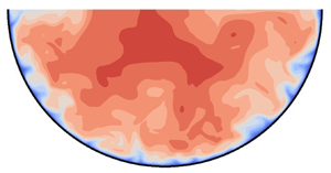
Although the rotational symmetry of the pipe is broken, laminar flow is invariant with respect to rotations about the pipe axis. This does not hold for turbulent flows. In figure 6 the normalised mean streamwise velocity is shown for $Re_{\tau } = 115$, 140, 180 and $460$. The distribution of the mean streamwise velocity depends on the Reynolds number. For $Re_{\tau }\geqslant 140$ we can observe the so-called ‘velocity-dip’ phenomenon, i.e. the maximum velocity – indicated by a plus in the plots – is not at the free surface. The distance of the velocity maximum from the surface increases within this Reynolds number range, which is further investigated below, see figures 7 and 8. These velocity distributions differ significantly from rotational symmetry. The general picture is in accordance with findings from higher Reynolds numbers in partially filled pipe flows (Knight & Sterling Reference Knight and Sterling2000; Clark & Kehler Reference Clark and Kehler2011; Yoon et al. Reference Yoon, Sung and Ho Lee2012; Ng et al. Reference Ng, Cregan, Dodds, Poole and Dennis2018) and rectangular open-duct flow (Tominaga et al. Reference Tominaga, Nezu, Ezaki and Nakagawa1989; Joung & Choi Reference Joung and Choi2009; Sakai Reference Sakai2016). For the very low, but still fully turbulent, Reynolds number $Re_{\tau }=115$ the velocity distribution is much closer to full-pipe flow and no ‘velocity-dip’ phenomenon can be detected. The same behaviour was observed by Sakai (Reference Sakai2016) for turbulent rectangular open-duct flow at marginal Reynolds numbers.

Figure 6.

Mean streamwise velocity $\bar {u}/u_b$ of $Re_{\tau }=115, 140$ (a,c) and $180,460$ (b,d). The symbol $+$ indicates the position of the velocity maximum.

Figure 7.

Distance $\Delta z^+$ from the free surface to the maximum mean streamwise velocity of $Re_{\tau }= 115$, 120, 140, 180, 230, 460 (${+}$, red). The symbol $\square$ represents data for rectangular open-duct flow from Sakai (Reference Sakai2016).

Figure 8.

Distance $\Delta z/R$ from the free surface to the maximum mean streamwise velocity of $Re_b= 3240$, 3364, 3874, 5198, 6874, 15452 (${+}$, red). The symbol $\square$ represents data for rectangular open-duct flow from Sakai (Reference Sakai2016). Including data from experiments: ${\blacklozenge }$ (blue) (Yoon et al. Reference Yoon, Sung and Ho Lee2012); ${\times }$ (blue) (Ng et al. Reference Ng, Cregan, Dodds, Poole and Dennis2018); ${\ast }$ (blue) (Clark & Kehler Reference Clark and Kehler2011); and ${\blacksquare }$ (blue) (Knight & Sterling Reference Knight and Sterling2000).

The distance of the maximum mean streamwise velocity from the free surface is shown in figure 7 in inner units. The data of a rectangular open-duct flow are shown for comparison (Sakai Reference Sakai2016), again taking the difference in cross-sectional area into account via the equivalent length scale $H_{eq}$. For the very low Reynolds numbers there is a slight difference, which can be explained by the different geometry and the vortex pattern, but for higher Reynolds numbers both cases match well. The distance in outer units can be compared with several other measurements of semifilled-pipe flows (Knight & Sterling Reference Knight and Sterling2000; Clark & Kehler Reference Clark and Kehler2011; Yoon et al. Reference Yoon, Sung and Ho Lee2012; Ng et al. Reference Ng, Cregan, Dodds, Poole and Dennis2018) at higher Reynolds numbers (figure 8). The experiment of Yoon et al. (Reference Yoon, Sung and Ho Lee2012), which is in the same Reynolds number range as our simulation, deviates from our data. Maybe their inflow length of $25 D_H$ is too short to have fully developed secondary flow. Note that Demuren & Rodi (Reference Demuren and Rodi1984) reported a fully developed secondary flow in a rectangular channel not before $70D_H$ from the inlet. On the other hand, the high-Reynolds-number cases would approximately follow the trend of our data. Taking all data into account, after a strong increase for small Reynolds numbers, the distance from the velocity maximum to the free surface $\Delta z(\bar {u}_{max}/R)$ seems to settle for larger Reynolds numbers between 0.3 and 0.4.

The magnitude of the normalised maximum mean streamwise velocity decreases with Reynolds number when normalised by $u_b$, see figure 9. This means that the momentum is more evenly distributed with higher Reynolds number, hence, the velocity distribution is more balanced and its peak, the maximum velocity, is less distinct. The data for $\bar {u}_{{max}}/u_b$ reported in the literature do not generally match to our results. While the maximum velocity measured by Ng et al. (Reference Ng, Cregan, Dodds, Poole and Dennis2018) continues our trend, the older measurements by Yoon et al. (Reference Yoon, Sung and Ho Lee2012), Clark & Kehler (Reference Clark and Kehler2011) and Knight & Sterling (Reference Knight and Sterling2000) largely deviate.

Figure 9.

Maximum mean streamwise velocity $\bar {u}_{{max}}/u_b$ of $Re_b = 3240$, 3364, 3874, 5198, 6874, 15452. Including experimental data: ${\blacklozenge }$ (blue) (Yoon et al. Reference Yoon, Sung and Ho Lee2012); ${\times }$ (blue) (Ng et al. Reference Ng, Cregan, Dodds, Poole and Dennis2018); ${\ast }$ (blue) (Clark & Kehler Reference Clark and Kehler2011); and ${\blacksquare }$ (blue) (Knight & Sterling Reference Knight and Sterling2000).

The ‘velocity-dip’ phenomenon can also be seen in figure 10, which shows the mean velocity profiles in the symmetry plane in inner units (for this plot, we used the local wall shear stress, obtained by the velocity gradient at the wall – see § 5). Near the wall, all profiles collapse to the linear law of the wall. For $Re_\tau \leqslant 140$, the profiles do not develop a logarithmic layer. For $Re_{\tau } = 180$ and $230$ a logarithmic layer can be observed, which reaches up to the velocity dip but the slopes are decreasing with increasing Reynolds number. Overall the Reynolds numbers seem to be too low to render a clear logarithmic behaviour such as is visible in higher Reynolds number pipe flows (El Khoury et al. Reference El Khoury, Schlatter, Noorani, Fischer, Brethouwer and Johansson2013), but they approach the standard log law $u^+=0.41^{-1} \ln (x_3^+) + 5.2$ at $Re_\tau =460$. At this Reynolds number a pronounced wake region develops beneath the velocity maximum. As the Reynolds number increases, the wake region becomes more distinct, which is visible also for experiments and simulations of full-pipe flow (Zagarola & Smits Reference Zagarola and Smits1997; El Khoury et al. Reference El Khoury, Schlatter, Noorani, Fischer, Brethouwer and Johansson2013) but has not been reported in experiments of semifilled-pipe flow so far (Ng et al. Reference Ng, Cregan, Dodds, Poole and Dennis2018).

Figure 10.

Mean streamwise velocity distribution $\bar {u}/u_{\tau,{local}}$ from the wall to the pipe centre at the vertical symmetry line of $Re_{\tau }= 115$, 120, 140, 180, 230, 460.

In outer units we can see that the velocity gradient is getting steeper close to the wall as the Reynolds number increases, see figure 11. The low Reynolds numbers increase monotonically and reach higher magnitudes. At high Reynolds numbers the velocity distribution is more complex. They have a less steep gradient from a wall distance of $z/R = 0.1$ on and the velocity-dip phenomenon in the bulk region. We can compare with the semifilled-pipe flows of Yoon et al. (Reference Yoon, Sung and Ho Lee2012) and Ng et al. (Reference Ng, Cregan, Dodds, Poole and Dennis2018). They basically show a similar velocity distribution, but for Yoon et al. (Reference Yoon, Sung and Ho Lee2012) the velocity-dip phenomenon is not as pronounced as it is for our simulation and the velocities in the symmetry plane are much higher than for any of our simulations when normalised by $u_b$. The velocity magnitude of the experiment by Ng et al. (Reference Ng, Cregan, Dodds, Poole and Dennis2018) fits quite well to our data and they also found an approximately zero gradient approaching the free surface.

Figure 11.

Mean streamwise velocity distribution $\bar {u}/u_{b}$ from the wall to the pipe centre at the vertical symmetry line of different $Re_b$. Including experimental data: ${\blacklozenge }$ (blue) (Yoon et al. Reference Yoon, Sung and Ho Lee2012); ${\times }$ (blue) (Ng et al. Reference Ng, Cregan, Dodds, Poole and Dennis2018).

4.2. Secondary flow

We are looking at the distribution of streamlines of the secondary flow over the cross-section, defined as lines of constant stream function $\psi$ and $\nabla ^2\psi = - \bar {\omega }_1$. We can find an alternating pattern of clockwise (red) and anticlockwise (blue) rotating vortices, which are symmetrically arranged with respect to the vertical bisector, see figure 12. The basic pattern does not change with Reynolds number. According to Grega et al. (Reference Grega, Hsu and Wei2002), the vortex in the mixed corner is also called the inner secondary cell and the centre vortex the outer secondary cell. For very low Reynolds numbers the vortices are almost equally strong and distributed over the whole circumference. The inner secondary cell gets smaller and moves towards the mixed corner when the Reynolds number is increased. In contrast, the centre vortex enlarges and is shifted towards the free surface. For higher Reynolds numbers the outer secondary cell has a negligible effect in the bottom region of the pipe. These observations are in line with the distribution of the in-plane velocity magnitude $\sqrt {u_2^2+u_3^2}/u_b$, shown as greyscale in figure 12. For friction Reynolds numbers smaller than $180$, the in-plane velocity is active over the whole cross-section. With higher Reynolds numbers the activity in the bottom region becomes less and the areas with high in-plane velocities concentrate at the free surface. For friction Reynolds numbers below $180$ the maximum in-plane velocity can be found in the inner secondary cell at $x_2/R \approx \pm 0.80$ and for higher $Re_{\tau }$ it is located in the outer secondary cell at $x_2/R \approx \pm 0.43$ directly at the free surface. The maximum in-plane velocity magnitude increases with Reynolds number from $1.3\,\%$ to $5.7\,\%$ of $u_b$ (note that the limits of the greyscales in the plot do not represent the exact range). This agrees well with data found in the literature for similar geometries (Tominaga et al. Reference Tominaga, Nezu, Ezaki and Nakagawa1989; Sakai Reference Sakai2016; Ng et al. Reference Ng, Cregan, Dodds, Poole and Dennis2018).

Figure 12.

Contours of stream function $\psi$ of mean cross-flow velocities $\overline {u_2}$ and $\overline {u_3}$ and as greyscale the velocity magnitude of $\sqrt {\overline {u_2}^2+\overline {u_3}^2}/u_b$ for $Re_{\tau }=115,140$ (a,b) and $180,460$ (b,d). The increments for the contour lines of $\psi$ are 0.003. For clarity the increments of $Re_\tau =460$ are doubled.

The pattern of the mean streamwise vorticity is similar to the one of the stream function, but does not truly reflect the mean vortex pattern, see figure 13. As it is the Laplacian of the stream function, the vorticity renders a smaller structure than the stream function. This is especially visible for the shear layers at the wall. As the Reynolds number increases the vorticity maxima are even farther shifted towards the free surface than the vortex centres deduced from the streamlines. Similar to the stream function, the mean streamwise vorticity is almost zero in the bottom region for higher Reynolds numbers, which indicates that the influence of the secondary flow could be very small in the lower part of a semifilled pipe.

Figure 13.

Mean dimensionless streamwise vorticity $\overline {\omega _1} R/u_b$ of $Re_{\tau }=115,140$ (a,c) and $180,460$ (b,d). The increments for the contour lines of $\overline {\omega _{1}} R/u_b$ are 0.04.

The distance of the vortex centres to the free surface ($+$) and the mixed corner ($\circ$) are shown in outer units over the bulk Reynolds number in figure 14(a). For both vortices the distances to the free surface and the mixed corner decrease with Reynolds numbers. For the outer secondary cell the distance to the mixed corner is approximately constant at ${\approx }0.6\Delta s/R$ for the higher Reynolds numbers, whereas the other distances are further decreasing. In wall units the outer secondary cell (blue) does not scale, whereas both distances of the inner secondary cell (red) scale well (figure 14b) especially at higher Reynolds numbers. Its distances range from $20$ to $50$ wall units. This is in agreement with the findings of Sakai (Reference Sakai2016) for rectangular open-duct flow in a similar range of Reynolds numbers. If the inner vortex continues to scale with inner units at higher Reynolds numbers one can expect that the inner secondary cell is getting very small compared with the radius of the pipe. Consequently, it would be more and more difficult to detect it by measurements with limited spatial resolution. This could explain why previous measurements in partially filled pipe flow only reported the outer secondary vortex (Clark & Kehler Reference Clark and Kehler2011; Ng et al. Reference Ng, Cregan, Dodds, Poole and Dennis2018).

Figure 14.

Normalised distance $\Delta s$ from the mixed corner ($+$) and free surface ($\circ$) to the minimum and maximum of the stream function $\psi$ in outer (a) and inner (b) units over $Re_{b}$ and $Re_{\tau }$, respectively. Red corresponds to the inner secondary vortex and blue to the outer secondary vortex.

As a measure for the strength of the secondary vortices, we have a look at the peak values of the stream function in the inner and outer secondary cells in figure 15. At the lowest two Reynolds numbers, both vortices exhibit the same amount of volume flux between the free surface and the vortex centre. At higher $Re_\tau$ the peak of the stream function reaches larger values in the outer vortex than in the inner vortex. While the stream function seems to saturate for larger Reynolds numbers in the outer vortex, it appears to attain its maximum at between $Re_\tau = 230$ and $460$ in the inner vortex.

Figure 15.

Normalised peak values of the stream function $\psi /(u_\tau /R)$ of the inner (${\circ }$, red) and the outer secondary cell (${+}$, blue) of $Re_{\tau }= 115$, 120, 140, 180, 230, 460.

The Reynolds dependency of the positions of the inner and outer secondary cells within the cross-section is shown in figure 16 by the locations of the vortex centres in one half of the duct. In agreement with the stream function distribution (cf. figure 12) the vortex centres move upwards as the Reynolds number increases. The inner secondary cell does always cover the position in the mixed corner and with decreasing size it moves farther into the mixed corner. For small Reynolds numbers the outer vortex centre is located close to the bottom and its circulation is similar to the one of the inner vortex. For moderate Reynolds numbers its position and the area it is covering change quickly. As the inner vortex becomes smaller, the size of the outer secondary cell becomes larger and moves to the centre. While the magnitude of the inner vortex vorticity strongly increases with Reynolds number (figure 13), its peak stream function remains bounded (figure 15). The peak values of the stream function in the outer cell grow stronger with Reynolds numbers than the one of the inner cell, whereas its vorticity only moderately increases. For higher $Re_\tau$ the position and the intensity of the outer secondary cell seems to stabilise, whereas the intensity of the inner secondary cell even decreases. Apparently, with increasing Reynolds number the outer secondary cell becomes more and more the dominating vortex. A similar observation has been made by Pirozzoli et al. (Reference Pirozzoli, Modesti, Orlandi and Grasso2018) for the case of a closed square duct. They observe a corner circulation with inner scaling and a core circulation scaling with the duct half-height, the latter being more and more dominant with increasing Reynolds number.

Figure 16.

Positions of the inner and outer secondary cell centres for $Re_{\tau }= 115$, 120, 140, 180,230, 460. Cell centres are defined as local minima and maxima of the stream function $\psi$. The symbol ${\circ }$ (red) corresponds to the inner secondary vortex and the symbol ${+}$ (blue) to the outer secondary vortex.

5. Wall shear stress

The local wall shear stress $\tau _{{w}}$ is an important parameter in terms of sedimentation and resuspension in sewage pipes. Its distribution over the perimeter can be seen as a footprint of the secondary flow. The wall shear stress is obtained by near wall velocity gradients. In figure 17(a) the distribution of the time-averaged wall shear stress $\tau _{{w}}/\tau _{0}$ around the wetted perimeter is shown for various Reynolds numbers, $\tau _{0}$ being the perimeter- and time-averaged wall shear stress. Independent of the Reynolds number the maxima can be found at the mixed corners. The local minima can be found at $\pm {\rm \pi}/4$ at the lowest Reynolds numbers and move towards the mixed corners when the Reynolds number is increased. At small Reynolds numbers ($Re\leqslant 140$) the distribution is nearly harmonic with a clear local maximum in the symmetry plane of the pipe. This local peak flattens and moves towards $\tau _{{w}}\approx \tau _{{0}}$ when the Reynolds number is increased. Eventually, secondary local maxima will be forming between the flat region and the minima. For small Reynolds numbers the maxima in the corners and in the symmetry plane have approximately the same magnitude. For increasing Reynolds numbers the difference between maxima and minima becomes larger while in the symmetry plane the wall shear stress tends to be $\tau _{{w}}\approx \tau _{{0}}$, reflecting the low activity of the secondary flow in the lower part of the pipe (cf. figure 12). The wall shear stress distribution can be explained with the secondary flow. In regions with a secondary flow pointing towards the wall, $\tau _{{w}}$ is high and when the secondary flow is directed away from the wall $\tau _{{w}}$ is small.

Figure 17.

(a) Normalised mean wall shear stress $\tau _{{w}}/\tau _0$ of $Re_{\tau }= 115$, 120, 140, 180, 230, 460. (b) Normalised mean wall shear stress $\tau _{{w}}/\tau _0$ of $Re_b= 15\,452$ and including experimental data: ${\ast }$ (blue) (Clark & Kehler Reference Clark and Kehler2011); and ${\blacksquare }$ (blue) (Knight & Sterling Reference Knight and Sterling2000).

In figure 17(b) our results are compared with the high Reynolds number experiments of Knight & Sterling (Reference Knight and Sterling2000) ($Re_b=110\,000$) and Clark & Kehler (Reference Clark and Kehler2011) ($Re_b=557\,000$, only data for one side available). They both match each other fairly well, but as they could not detect the inner secondary cell within their measurements, they also do not show a global wall shear stress maximum at the mixed corner. Instead, they found the global minimum at the mixed corner and the global maximum at the centre bottom.

In order to quantify the level of fluctuations of the wall shear stress we obtained the instantaneous local wall shear stresses from velocities interpolated to a wall distance of $\Delta r^+=2$. The r.m.s. of its fluctuations normalised by the global wall shear stress are plotted in figure 18 along the perimeter. In general, the distribution resembles the mean wall shear stress distribution with its maxima at the mixed corners, followed by a minimum and a plateau in the centre. Hence, the largest fluctuations in wall shear stress occur in the mixed corner. With increasing Reynolds number the local minimum moves towards the mixed corner as was observed for the mean wall shear stress. The r.m.s. level in the centre increases with Reynolds number and nearly reaches $\tau _{w,rms}/\tau _0\approx 0.4$, a value that was observed in channel and pipe flows at high Reynolds numbers (Alfredsson et al. Reference Alfredsson, Johansson, Haritonidis and Eckelmann1988; El Khoury et al. Reference El Khoury, Schlatter, Noorani, Fischer, Brethouwer and Johansson2013). The local fluctuations in the mixed corners are approximately 1.2–1.7 times stronger than in the centre of the perimeter. Moreover, they reach approximately the value by which the time-averaged wall shear stress exceeds the perimeter-averaged one.

Figure 18.

Normalised r.m.s. of wall shear stress fluctuations $\tau _{{w,rms}}/\tau _{{0}}$ over the perimeter for $Re_{\tau }=115,120,140,180,230,460$.

In the mixed corner the secondary flow points towards the pipe's wall which explains the large wall shear stress values in the mixed corner. The first wall shear stress minimum is close by the location where the flow separates from the perimeter and marks the end of the inner vortex. This is demonstrated in figure 19 in which both locations are plotted in dependence of the Reynolds number. At the lower Reynolds number the separation point is approximately 10 wall units farther away from the mixed corner than the wall shear stress minimum. The distance from the mixed corner to the first wall shear stress minimum and the separation point has its minimum at $Re\approx 230$. At $Re_\tau = 460$ the distance to both points increases and reaches ${\approx }90^+$ and $65^+$, respectively. More data at higher Reynolds numbers would be necessary to elucidate a scaling here.

Figure 19.

Azimuthal distance in wall units $\Delta s^+$ from mixed corner to first minimum of wall shear stress (${+}$, red) and to the separation point of the secondary flow (${\circ }$, blue) for $Re_{\tau }=115$, 120, 140, 180, 230, 460.

In pipe flow, wall shear stress fluctuations are linked to the appearance of streaks in instantaneous near-wall streamwise velocities, which are plotted in figure 20 at a constant distance from the wall of $10^+$. An alternating pattern of low- and high-speed streaks can be detected independent of $Re$. In outer units individual streaks become smaller with increasing Reynolds number, as they scale with inner units, having an average spacing of $100^+$ in channel flow (Kim, Moin & Moser Reference Kim, Moin and Moser1987). This streak spacing would give rise to approximately $3.5$ high-speed streaks fitting in the perimeter at $Re_\tau =115$ and to $14.5$ streaks at $Re_\tau =460$. A similar approach was employed by Pinelli et al. (Reference Pinelli, Uhlmann, Sekimoto and Kawahara2010) for a rectangular closed duct, which will be further referred to at the end of this section. The instantaneous velocity distributions do not contradict such a spacing. The wall shear stress peak in the mixed corners, i.e. at $\pm \frac {1}{2}{\rm \pi}$, can hardly be seen as increased levels in the instantaneous velocity distribution. There are strong fluctuations of the streamwise velocity at a $10^+$ wall distance which do not seem to differ in the mixed corners from the centre of the channel.

Figure 20.

Instantaneous normalised streamwise velocity $u_1/u_b$ at a constant distance of 10 wall units from the wall over the channel length for $Re_\tau =115,140,180,460$ (a–d).

The observation that the time-averaged wall shear stress distribution is not visible in instantaneous velocity distributions is supported by figure 21 in which cross-sectional distributions of the instantaneous streamwise velocity are plotted. The uplift of low-speed fluid from the wall can be clearly seen at specific spots along the circumference. With increasing Reynolds number, more and smaller uplift events can be seen, as expected. There is no specific structure visible in the mixed corners. However, in the higher Reynolds numbers, the velocity dip is clearly visible.

Figure 21.

Instantaneous normalised streamwise velocity $u_1/u_b$ over the cross-section for $Re_\tau =115,140$ (a,c) and $180,460$ (b,d).

In order to evaluate the character of the wall shear stress distribution, we computed running averages of the wall shear stress at a fixed streamwise position using an averaging time of one flow-through time $L/u_b$. These are plotted for $40 L/u_b$ (figure 22). In this representation, the short-time fluctuations which obscured the long-term variations of the wall shear stress are not visible. It becomes obvious that the running averages reveal large wall shear stresses in the mixed corners for most of the time. In addition to these wall shear stress maxima in the mixed corners, local minima occur next to them. The variations in the centre appear more random and only a few extreme values show up. In a similar manner, Pinelli et al. (Reference Pinelli, Uhlmann, Sekimoto and Kawahara2010) investigated the velocity streak behaviour for the solid corner in a rectangular closed duct with a local wall shear stress minimum appearing in the vicinity of the solid corner. The Reynolds dependency of their velocity streaks is analogous to our case, with the difference that in our case the fixed peak is not in the solid corner, but at the free surface. Overall the evaluation of the wall shear stress and near wall velocity streaks suggests that the mixed corner vortex is not a stable vortex – in the sense that it rotates constantly in the same direction – but results from an averaging of many individual uplift and downwash events which are present in wall-bounded turbulence. This is in good agreement with the findings of Sakai (Reference Sakai2016), who did a statistical analysis on the probability of vortex positions in rectangular open-duct flow. He showed that in the mixed corner mostly vortices are present, that rotate towards the wall at the free surface, which would generate a similar wall shear stress pattern like our running averaged wall shear stress distribution.

Figure 22.

Temporal distribution of the normalised running-averaged wall shear stress $\tau _{{w}}/\tau _0$ over the perimeter for $Re_{\tau }=180$. One time instant represents the running-averaged $\tau _w$ over a period of $L/u_b$. Total time interval is 40 $L/u_b$.

It seems that for all Reynolds numbers the low- and high-speed streaks appear, which can be associated with quasi-streamwise vortices. These structures are scaling in inner units, i.e. with a streak spacing of around $100\nu /u_\tau$. In the low-Reynolds-number cases ($Re_\tau \leqslant 140$) they fill the whole cross-section and their movement is restricted. It seems that in this range, only four streaks fit into the semifilled pipe. This leads to a preferential position of the streamwise vortices which can explain the mean secondary flow cells and the harmonic distribution of the mean wall shear stress. At higher Reynolds numbers ($Re_\tau \geqslant 180$), the time-averaged cells seem to be lifted from the lower part of the semifilled pipe towards the free surface (see figure 12). This might be a result of a larger variability of the streaks in circumferential direction which leads to averaging out of the low- and high-speed zones in the statistical sense. This can explain the plateau in the wall-shear stress. Similar observations for a comparable range of Reynolds numbers were made by Pinelli et al. (Reference Pinelli, Uhlmann, Sekimoto and Kawahara2010) for a rectangular closed-duct flow. In the mixed corners there is always a low- or a high-speed streak, since at the free surface the in-plane velocity vector always points towards or from the corner for kinematical reasons, thus fixing the streak there. From figure 22 we can infer that the flow has the preference to point towards the mixed corners, thus transporting high-speed fluid towards the corners.

6. Reynolds stresses

In this section we examine the spatial distribution of the Reynolds stresses. First, we examine the Reynolds number dependence of the Reynolds stress profiles in the symmetry line (figure 23). For the normal stresses, we plot the r.m.s. of the velocity fluctuations. Between their maxima and the wall, all profiles share a high degree of similarity with those found in full-pipe flow. The streamwise normal stresses $\overline {u_1'^2}$ are largest and peak at around $x_3^+ \approx 15$. The position is rather independent of the Reynolds number while the peak value slightly increases. Similarly to the observations of El Khoury et al. (Reference El Khoury, Schlatter, Noorani, Fischer, Brethouwer and Johansson2013), there is a strong increase of the other Reynolds stresses in inner coordinates with Reynolds number. Note that in the symmetry line, $u_3$ is the radial component and $u_2$ is the azimuthal component. The most prominent difference to the Reynolds stress distributions in full-pipe flow can be found near the free surface at which the velocity component perpendicular to the surface $u_3$ is strongly damped and the other two components are amplified. The minima of $u_{1,rms}$ are approximately $0.75 u_\tau$ and the ones of $u_{2,rms}$ are a little smaller. The distances of these minima from the free surface seem to coincide in inner units while the thickness of the damping layer of $u_{3,rms}$ to the free surface is much thinner. The shear stress $\overline {u_1'u_3'}$ does go to zero at the free surface, but changes its sign beforehand and shows a small positive maximum close to the free surface. The deviation from the full pipe profile above the maximum demonstrates that the Reynolds shear stress does not follow the linear trend between its maximum and the centre, which is typical for turbulent flow in a full pipe. This departure can be explained with the momentum transport by the secondary flow. The Reynolds stress distributions presented by Ng et al. (Reference Ng, Cregan, Dodds, Poole and Dennis2018) are similar to ours. Unfortunately, they did not give their results in inner units. However, their measured maxima seem to be smaller than ours when normalised in bulk units ($\overline {u_1'^2}/u_b^2\approx 0.01$ to $\overline {u_1'^2}/u_b^2\approx 0.025$ for $Re_\tau = 460$).

Figure 23.

The r.m.s. of the velocity fluctuations $u_{{1,rms}}/u_\tau, u_{{2,rms}}/u_\tau, u_{{3,rms}}/u_\tau$ and Reynolds shear stress $\overline {u_1'u_3'}/u_\tau ^2$ in inner units in the vertical symmetry line of $Re_{\tau }= 115$, 120, 140, 180, 230, 460. The straight black lines represent full-pipe flow from our DNS. Please note that for the shown data along the vertical symmetry line the Cartesian coordinates in $x_2$ and $x_3$ directions are equal to the polar coordinates $\theta$ and $r$, respectively.

The cross-sectional distributions of the Reynolds stresses reveal that the levels of turbulence intensities are equally high around the perimeter up to the area of the mixed corner – see figure 24 showing the Reynolds normal and shear stresses for $Re_{\tau }=180$ in polar coordinates. We plot the sum of the cross-stream normal stresses for clarity. The streamwise stresses have considerably larger values than the other stresses, demonstrating that the TKE (not shown here) is dominated by $\overline {u_1'^2}$. The minimum of $\overline {u_1'^2}$ appears at the location of the mean streamwise velocity maximum. The layer of large values of $\overline {u_1'^2}$ around the perimeter has local minima in the inner vortex where the secondary flow is parallel to the wall. A local maximum occurs at the location at which the secondary flow points away from the wall.

Figure 24.

Normalised r.m.s. of velocity fluctuations $u_{{1,rms}}/u_\tau$, $(u_{{r,rms}}+u_{{\theta,rms}})/u_\tau$ (a,b), $\overline {u_1'u_r'}/u_\tau ^2$, $\overline {u_1'u_\theta '}/u_\tau ^2$ (c,d) for $Re_{\tau }= 180$.

The streamwise Reynolds stress and the sum of the cross-stream stresses are nearly homogeneous in azimuthal direction in the lower part of the pipe within $\pm 45^\circ$ from the bisector. This is consistent with the observation that the secondary flow is weak in the lower part of the flow and suggests that the flow near the lower wall could behave like a normal pipe flow. This conjecture is partly supported by the shear stress $\overline {u_1'u_\theta '}$ which is essentially zero in the lower part. However, the distribution of $\overline {u_1'u_r'}$ is not fully homogeneous in the lower part. We don't show $\overline {u_r'u_\theta '}$ because it is very small throughout the whole cross-section.

The sum of the cross-stream components shows their maximum at approximately $0.25R$ from the wall with a stronger contribution of the azimuthal component at the bottom and along the wall, whereas the radial component has its maximum at the free surface. The effect of the mixed corner on the normal stresses $\overline {u_1'^2}$ and $(u_{{r,rms}}+u_{{\theta,rms}})$ is primarily a damping. The shear stresses, however, are strongly affected near the mixed corner. The magnitude of $\overline {u_1'u_r'}$ peaks in the area below the inner vortex where the secondary flow points away from the wall. The magnitude of $\overline {u_1'u_\theta '}$ peaks in the region where the corner vortex flow is parallel to the wall. Both of those peaks could be linked to strong fluctuations of the corner vortex associated with the dynamics of the near-wall streaks discussed in the previous section.

In order to better understand the Reynolds stress distribution, the anisotropy of the Reynolds stress tensor will be evaluated by the so-called Lumley or turbulence triangle. This is done in figure 25 in the symmetry line according to its invariants $\eta$ and $\xi$. They are defined by the eigenvalues of the Reynolds stress tensor: $\eta ^2=\frac {1}{3}(\lambda _1^2+\lambda _1\lambda _2+\lambda _2^2)$ and $\xi ^3 = -\frac {1}{2}(\lambda _1\lambda _2(\lambda _1+\lambda _2))$ (Pope Reference Pope2000). Starting from the wall, the general behaviour first follows the distribution of a channel flow (see Pope (Reference Pope2000)) until a turning point is reached. Directly at the wall the streamwise component is dominant and the azimuthal component is weakly present. At a wall distance of $10^+$ the flow tends towards the one-component state. This is more pronounced at lower Reynolds number. With increasing wall distance the Reynolds stresses move towards the isotropic state until they reach a sharp turning point, which is closer at the isotropic state when the Reynolds number is higher. This turning point is the point at which the boundary condition of the free surface starts to damp the vertical component and which is marked by a local minimum in the streamwise and spanwise Reynolds stresses. Upwards from this point, the Reynolds stresses have to move towards the two-component state as the vertical component is zero at the free surface. For Reynolds numbers $\geqslant 140$ the two-components at the free surface are equally strong, whereas for lower $Re_\tau$ the second component is less dominant. For the higher $Re_\tau$ an oblate-spheroid-shaped anisotropy appears underneath the free surface.

Figure 25.

Lumley triangle in the $\eta$–$\xi$ plane of the Reynolds stress tensor in the vertical symmetry line for $Re_\tau = 115$, 120, 140, 180, 230, 460.

Emory & Iaccarino (Reference Emory and Iaccarino2014) proposed to link the position in the anisotropy map to a colour code, which can be used to visualise the turbulence state over the entire cross-section (figure 26a). The specific colour map is defined in figure 26(b). The nearly one-component turbulence (red colour) spreads along the whole perimeter including the inner vortex region. From the Reynolds stress plots it becomes clear that the streamwise component is dominant in this region. Farther away from the wall there is another ring-like area in which the Reynolds stresses move towards the three-component state (magenta). The area of the velocity maximum is characterised by a state which is near the three-component limit (blue). Near the free surface, a layer behaves differently. Here, the damping of the vertical fluctuations changes the flow state to a two-component limit (yellow and green). When moving from the mixed corner to the centre, the state changes gradually from a one-component (red) to two-component (green) state.

Figure 26.

Anisotropy componentiality of Reynolds stresses over the cross-section for $Re_{\tau }=180$ (a). Colour map according to nonlinear anisotropy invariant map (b).

Moreover, Einstein & Li (Reference Einstein and Li1958) found out that the anisotropy of the in-plane Reynolds stresses is generating streamwise vorticity, hence, turbulence-induced secondary flow. This conclusion can be drawn from the equation for the mean streamwise vorticity (as follows), simplified for a straight and steady flow:

(6.1)\begin{align} \bar{u}_2 \frac{\partial\bar{\omega}_1}{\partial x_2} + \bar{u}_3 \frac{\partial\bar{\omega}_1}{\partial x_3} = \frac{\partial^2}{\partial x_2 \partial x_3}(\overline{u_{3}'^{2}} - \overline{u_{2}'^{2}}) + \left(\frac{\partial^2}{\partial x_3^2} - \frac{\partial^2}{\partial x_2^2}\right)(-\overline{u'_3 u'_2}) + \frac{\partial}{\partial x_j}\left(\nu\frac{\partial\bar\omega_1}{\partial x_j}\right). \end{align}

The convection terms on the left-hand side are balanced by gradients of the Reynolds shear and normal stress terms and a vorticity dissipation term. The Reynolds shear and normal stress terms have been denoted as vorticity dissipation and generation, respectively (Nezu & Nakagawa Reference Nezu and Nakagawa1993; Nikora & Roy Reference Nikora and Roy2012). It is obvious that this denomination is not invariant with respect to coordinate transformations. As a sum, however, they are responsible for the production (or destruction) of streamwise vorticity (Einstein & Li Reference Einstein and Li1958; Nezu & Nakagawa Reference Nezu and Nakagawa1993). In figure 27 one can see the sum of the Reynolds stress terms which is approximately zero over the whole cross-section apart from a small region at the mixed corners. A negative value of vorticity production leads to a clockwise rotating vortex and vice versa. Hence, following the derivation of Einstein & Li (Reference Einstein and Li1958) and Nezu & Nakagawa (Reference Nezu and Nakagawa1993), we can conclude that the mixed corner region is responsible for the generation of the mean secondary flow in semifilled-pipe flow, which emphasises the role of the inner secondary cell.

Figure 27.

Sum of normalised vorticity generation and dissipation ${\partial ^2}/{\partial x_3 \partial x_2}(\overline {u_3'^2}-\overline {u_2'^2})+({\partial ^2}/{\partial x_3^2}-{\partial ^2}/{\partial x_2^2})(-\overline {u_3'u_2'})R^2/u_{\tau }^2$ for $Re_{\tau }=180$.

While the general distribution is similar to rectangular open-duct flow (Kara, Stoesser & Sturm Reference Kara, Stoesser and Sturm2012), in rectangular open-duct flow the mean streamwise vorticity is also produced at rigid, solid–solid, corners. The total secondary flow generated there is similarly strong as for semifilled-pipe flow. This means the inner secondary cell alone is able to produce a similarly strong secondary flow which underlines the prominent role the mixed corner plays in open-duct flows. In the next section we draw the attention to the aspect of how the secondary flow obtains its kinetic energy, highlighting another perspective to the question of how turbulence-induced secondary flow is generated in semifilled-pipe flow.

7. Path of kinetic energy

Nikora & Roy (Reference Nikora and Roy2012) have proposed a path of kinetic energy highlighting the perspective of the mean kinetic energy (MKE) ($K=1/2 (\overline {u_1}^2+\overline {u_2}^2+\overline {u_3}^2)$) budget on the generation of mean secondary flow. It is based on the component-wise MKE budget for steady, straight and uniform flow in which $u_1$ is the streamwise and $u_2$ and $u_3$ are the secondary velocity components (7.1) and (7.2), as follows:

(7.1)\begin{align} 0&=\underbrace{-\bar{u}_j\frac{\partial}{\partial x_j}\left(\frac{\bar{u}_1^2}{2}\right)}_{\substack{\text{convection}\\ C_1}} - \underbrace{\frac{\partial}{\partial x_j}(\bar{u}_1 \overline{u_1'u_j'}) + \nu\frac{\partial^2}{\partial x_j^2}\left(\frac{\bar{u}_1^2}{2}\right) }_{\substack{\text{transport}\\ T_1 = T_{1,turb} + T_{1,visc}}} + \quad \underbrace{g_1\bar{u}_1}_{\substack{\text{energy input}\\\text{by volume force}\\E_{{in}}}} \nonumber\\ &\quad + \underbrace{\overline{u_1'u_j'}\frac{\partial \bar{u}_1}{\partial x_j}}_{\substack{\text{production of TKE}\\ P_1}} + \underbrace{\nu\left(\frac{\partial \bar{u}_1}{\partial x_j}\right)^2}_{\substack{\text{dissipation}\\ \bar{\epsilon}_1}}, \quad\mathrm{with}\ j = 2,3 , \end{align}

(7.2)\begin{align} 0&=\underbrace{-\bar{u}_j\frac{\partial}{\partial x_j}\left(\frac{\bar{u}_2^2 + \bar{u}_3^2}{2}\right)}_{\substack{\text{convection}\\ C_{2,3}}} \underbrace{- \frac{1}{\rho}\left(\frac{\partial \bar{p}}{\partial x_2}\bar{u}_2 + \frac{\partial \bar{p}}{\partial x_3}\bar{u}_3\right) -\frac{\partial}{\partial x_j}(\bar{u}_2 \overline{u_2'u_j'} + \bar{u}_3 \overline{u_3'u_j'}) + \nu \frac{\partial^2}{\partial x_j^2}\left(\frac{\bar{u}_2^2 + \bar{u}_3^2}{2}\right)}_{\substack{\text{transport}\\ T_{2,3} = T_{2,3,press} + T_{2,3,turb} + T_{2,3,visc}}}\nonumber\\ & \quad+ \underbrace{\overline{u_2'u_j'}\frac{\partial \bar{u}_2}{\partial x_j} + \overline{u_3'u_j'}\frac{\partial \bar{u}_3}{\partial x_j}}_{\substack{\text{production of TKE}\\ P_{2,3}}} + \underbrace{\nu\left(\frac{\partial \bar{u}_2}{\partial x_j}\right)^2 + \nu \left(\frac{\partial \bar{u}_3}{\partial x_j}\right)^2}_{\substack{\text{dissipation}\\ \bar{\epsilon}_{2,3}}} , \quad \mathrm{with}\ j = 2,3. \end{align}

Please note, since the steady volume force driving the flow $g_i$ acts only in the streamwise direction ($g_2=g_3=0$), the energy input $E_{in}$ appears only in the MKE budget for the streamwise component. In a gravity-driven flow, the term $g_3\overline {u_3}$ would be in equilibrium with the hydrostatic pressure, hence no energy input would occur in the velocity component $u_3$. The kinetic energy is redistributed in space by the convection term $C_1$ and the turbulent and the viscous transport terms $T_1$. Parts of it are directly dissipated ($\bar {\epsilon }_1$) and other parts are transferred to TKE ($k=1/2 (\overline {u_1'^2}+\overline {u_2'^2}+\overline {u_3'^2})$) via the production term $P_1$. Note that there is no direct intercomponent transfer term from the streamwise to the secondary velocity components. The kinetic energy enters the mean secondary flow in a two-step process. First the production terms $P_1$ transfer energy to TKE, where it is partly dissipated, redistributed in space and spread among the fluctuation components. Second, some of the remaining part is transferred to the secondary flow $(\overline {u_2}^2+\overline {u_3}^2)$ by the terms $\overline {u_2'u_j'}({\partial \bar {u}_2}/{\partial x_j})$ and $\overline {u_3'u_j'}({\partial \bar {u}_3}/{\partial x_j})$ ($P_{2,3}$). The secondary MKE is redistributed in space, directly dissipated or transferred back to TKE by the other terms in (7.2). In order to verify the suggested path of kinetic energy and to explicitly apply it to the semifilled-pipe flow, all important terms of the path will be analysed in the following.

First of all the budget of the MKE shall be validated by checking the residuum of the primary and in-plane components of the MKE budget at the free surface, where strong convection is present. The residuum ($RES$) is the black solid line in figure 28. Hence, for the primary MKE budget the maximum residuum is less than $2\,\%$ of the maximum of other terms, apart from the very first cell at the wall. For the secondary components the residuum is also less than $2\,\%$ compared with the other terms in most of the cross-section apart from the first cells at the wall.

Figure 28.

Primary (a,c) and secondary component (b,d) terms of MKE budget (a,b) and only the transport terms as sum and individually (c,d) taken four wall units below and parallel to the free surface for $Re_{\tau }=180$.

Looking at the magnitude of the budget terms near the free surface, it is obvious that the primary MKE is highly dominating the total MKE budget. Very close to the mixed corner the viscous transport balances the direct dissipation. Moving away from the mixed corner the production, convection and turbulent transport also contribute to the budget. In the bulk region the energy input is mainly balanced by the convection and the turbulent transport. Focusing on the secondary component mostly the terms of production, convection, pressure and turbulent transport are balancing each other. A more detailed look at the budget is presented via the expansion of selected terms over the whole cross-section.

We first inspect the distributions of the primary and secondary MKE and TKE, see figures 29 and 23(a,b). The distribution of the primary MKE, $\bar {u}_1^2$, is similar to the distribution of the streamwise velocity (figure 6) displaying large values of MKE in the pipe's centre and below where the velocity maximum can be found. The secondary MKE has peak values less than one per mille of the primary MKE. Two peaks can be found at the free surface symmetrically between the pipe axis and the mixed corners. Smaller local peaks can be found around the corner vortex. The values in figure 23 would need to be squared in order to get the right magnitude for the TKE, but qualitatively the distribution does not change. For the readers’ convenience we recall briefly the most important points. The largest values of primary TKE, $\overline {u'^2}$, can be found in a band along the perimeter at a wall distance of approximately 15 wall units. The maxima of the secondary TKE are distributed along the perimeter at larger wall distances than the maxima of the primary TKE. Below, we will discuss the terms in the balance equation for the MKE.

Figure 29.

Mean kinetic energy $K$ of primary component (a) and secondary components (b) for $Re_{\tau }=180$ normalised by $u_\tau ^2$.

The primary MKE is generated by the gravity input term, see (7.1), which is proportional to the streamwise velocity. The production terms of TKE are displayed in figure 30. It is obvious that the production of primary TKE is similarly distributed as the primary TKE itself. It seems to be very similar to the distribution in a standard turbulent pipe flow with a nearly homogeneous distribution around the perimeter. On the other hand, the production term of secondary TKE is strong at the free surface, where the secondary MKE has its maxima. While the production term of primary TKE is consistently negative in the MKE balance equation (energy is transferred from the mean flow to the turbulent fluctuations), its counterpart for secondary TKE changes sign. This means that in the regions where the production term is positive, energy is transferred from the fluctuations to the mean secondary flow and vice versa.

Figure 30.

Production $P$ of primary component (a) and secondary components (b) for $Re_{\tau }=180$ normalised by $R/u_\tau ^3$.

We can observe that kinetic energy is transferred to the mean secondary flow only in two regions symmetrically around the pipe's axis being located at the stagnation point at the free surface marking the boundary between the inner and outer vortices. The mean secondary flow points away from this stagnation point, thus giving rise to a positive production term $\overline {u_2'u_2'}({\partial \overline {u_2}}/{\partial x_2})$ in the MKE balance. In the pipe centre, the secondary flow from both sides of the pipe point to each other and are redirected downwards. This situation generates a negative production term in the MKE balance and kinetic energy is transferred back from the secondary MKE to the secondary TKE. A similar effect can be observed at the lower boundary of the inner vortex where the secondary flow is directed away from the wall. Here as well, transfer from secondary MKE to TKE is indicated by a negative production term. We can, therefore, infer that a part of the kinetic energy that the mean secondary flow receives at the free surface is passed back to the turbulent secondary flow.

A condition of having a non-zero transfer between secondary MKE and TKE is that the vertical fluctuations are damped near the free surface. This can be seen by rewriting the production term of secondary TKE in (7.2) neglecting the shear production – which is small – and using the continuity equation ($\partial \bar {u}_2/\partial x_2 = -\partial \bar {u}_3/\partial x_3$):

(7.3)\begin{equation} \overline{u_2'u_2'}\frac{\partial \bar{u}_2}{\partial x_2} +\overline{u_3'u_3'}\frac{\partial \bar{u}_3}{\partial x_3} = \left(\overline{u_2'u_2'} - \overline{u_3'u_3'}\right) \frac{\partial \overline{u_2}}{\partial x_2} . \end{equation}

At the free surface, the vertical fluctuations $u_3'$ are damped and the horizontal fluctuations $u_2'$ are amplified – compare figures 24 and 23. Thus, in contrast to an isotropic turbulence structure, the normal stress difference in (7.3) increases at the free surface enabling exchange of kinetic energy between the mean and the fluctuating velocities.

In figure 31 the primary and secondary terms of the convection, the summed transport terms and dissipation of the MKE budget are shown. Overall, all individual distributions have in common that their high intensities are mostly along the perimeter, in the mixed corner and along the free surface. There are no high intensities where the mean streamwise flow has its maximum. The convection of primary kinetic energy is effectuated by the secondary flow. It has large values in the mixed corner, positive at the upper side of the inner secondary cell and negative at the lower side of the vortex. This means that the secondary flow transports high energetic fluid into the mixed corners and low energetic fluid from below the inner vortex into the bulk. Within the area in which the convection term is negative (marked as blue) the streamwise velocity and, therefore, the primary MKE increases along the streamlines.

Figure 31.

Convection $C$ (a,b), transport terms $T$ (c,d) and dissipation $\bar {\epsilon }$ (e,f) of primary component (a,c,e) and secondary components (b,d,f) of the MKE budget for $Re_{\tau }=180$ normalised by $R/u_\tau ^3$.

The transport terms lump together viscous, pressure and turbulent transport which all contribute to a spatial redistribution of the MKE. Along the perimeter the transport terms have a small layer of high positive intensities presumably from viscous transport of momentum towards the wall. This effect seems to be strongest near the mixed corner. Around the inner vortex, two patches appear obviously counteracting the convective term. Overall the primary transport terms are carrying primary MKE from the pipe centre (negative) towards the walls (positive), where it is either dissipated or transferred to TKE.

The convection of the secondary MKE is negligibly small over the cross-section in comparison with the other terms. The largest magnitudes of the secondary transport terms are smaller than the magnitudes of the primary transport by a factor of ${\sim }100$, which is not surprising given the ratio of primary to secondary MKE being approximately 1500 (cf. figure 29). They are mostly active in the mixed corner and in the centre of the free surface, negative where stagnation and positive where separation points of the mean secondary flow exist. As seen in figure 28 the transport terms balance the production terms, hence, where secondary MKE is produced it is transported away and where TKE is produced secondary MKE is needed and brought to that location by the secondary transport terms, especially the turbulent transport. The primary direct dissipation acts in the vicinity of the wall with its highest intensities in the mixed corner. The secondary components of the direct dissipation are very small and visible only along the wall where the inner secondary cell is located and in a small region at the bisector of the mixed corner. Please note that primary and secondary terms have different scales. Moreover, please keep in mind that the overall energy input is contributed proportional to the mean streamwise velocity by a constant pressure force as external force. An equilibrium state has been reached, to which every term contributes.

The path of kinetic energy is further illustrated by the cross-section integrated terms of the kinetic energy budgets (figure 32). Terms redistributing kinetic energy in space, such as convection and the transport terms, vanish after integration. Approximately two thirds of the kinetic energy input are dissipated directly by the mean streamwise velocity $\overline{\epsilon}_1$ which can be explained by the relatively low Reynolds number ($Re_\tau = 180$). One third is transferred to TKE and mainly dissipated by the dissipation of TKE $\epsilon = \frac{\nu}{2}\sum_{ij}\overline{\left(\frac{\partial u_i'}{\partial x_j}+\frac{\partial u_j'}{\partial x_i}\right)^2}$. Only a very small fraction, less than one per mille of the total kinetic energy flux is fed to the secondary flow in regions in which the production term is positive ($P_{2,3}>0$). More than two thirds of this energy is transferred back to TKE in regions in which the production term is negative ($P_{2,3}<0$). The difference ($0.7$ per mille) is dissipated by the mean secondary flow $\overline{\epsilon}_{2,3}$. Please note, $\overline{\epsilon} = \overline{\epsilon}_{1} + \overline{\epsilon}_{2,3}$. The magnitudes of the energy fluxes reflect the ratios of the kinetic energies of which the secondary MKE has amplitudes approximately 1500 times smaller than the primary MKE and approximately 10 times smaller than the secondary TKE. Nevertheless, the secondary flow has a strong impact on the distribution of the statistical quantities, especially the time-averaged wall shear stress.

Figure 32.

Path of kinetic energy for $Re_{\tau }=180$. Integrated values normalised by the energy input $g \bar {u}_1$.

The path of the kinetic energy in figure 32 is complemented with values for other Reynolds numbers in figure 33. As expected, with increasing Reynolds number direct dissipation decreases and the share of energy transferred to TKE increases. We see that independent of the Reynolds number the turbulent dissipation is nearly equal to the production of TKE. The energy exchange between turbulence and secondary flow, $P_{2,3}$ gets stronger with increasing Reynolds number and seems to saturate for larger $Re_\tau$. This behaviour is similar to the behaviour of the peak values of the stream function, see figure 15. The forward transfer from the turbulence to the secondary flow $P_{2,3}>0$ is always larger than the backward transfer $P_{2,3}<0$. The difference is the energy dissipation by the secondary flow which has a nearly invisible share of the total energy balance.

Figure 33.

Cross-section integrated values of $P_1$, $\bar {\epsilon }$ and $\epsilon$ (a) and $P_{2,3>0}$ and $P_{2,3<0}$ (b) for $Re_{\tau }= 115$, 140, 180, 230, 460 normalised by the energy input $g \bar {u}_1$.