Basic units of study

Although host–parasite interactions are dynamic processes, a snapshot survey represents the process frozen at an instant of time. This snapshot provides an assemblage of N hosts and P parasites. In the ADD model, host and parasite populations are systematically scanned and the proportion of parasites associated with each stratum of host population can be identified. This leads to basic units of study for the re-formulated binomial and inequality application, as follows.

The population of N hosts under consideration are divided into two groups, A and B, comprising N ₁ and N ₂ hosts:

• N ₁ hosts each with parasite numbers up to the threshold (A)

• N ₂ hosts each with parasite numbers above the threshold (B)

The total number of hosts, N, is:

and the corresponding proportions in the groups are:

(1)

Measures of infection are determined for group B, which forms a cohort of hosts with each individual host harbouring parasites above a threshold level.

The total parasite population (P) consists of P ₁ parasites carried by N ₁ hosts (group A), and P ₂ parasites carried by the N ₂ hosts (group B). The total number of parasites, P, is:

(2)

The mean intensity of infection is:

(3)

Binomial dichotomy and re-formulated negative binomial distribution

The actual parasite number, i, harboured by individual hosts may be in the range 0 ≤ i ≤ ∞. By considering the level of infection at a threshold i = i*, the host population is demarcated into groups A and B, with individual hosts in A carrying 0 ≤ i ≤ i*, and in B carrying i>i* parasites. Groups A and B comprise N ₁/N and N ₂/N fractions of the host population. Therefore the traditional negative binomial distribution is transformed as follows:

(4)

where N ₁/N refers to the proportion of hosts with individual host carrying 0 ≤ i ≤ i* parasites and m is the mean intensity in the total host population. The parameter k _i>i* in Equation 4 gives the measure of dispersion of hosts harbouring parasite numbers above the threshold (i>i*). The proportion N ₂/N is described as prevalence p _i>i* which is the re-formulated NBD applied by Pal & Lewis (Reference Pal and Lewis2004). In traditional investigations, the prevalence is defined at i>0, and hence should be represented as p _i>0, although it appears with no subscript attached.

Aggregation

In economics, differential concentrations of wealth are at the heart of inequality in the context of distribution. However, similarities exist in the distribution of parasites in host communities. In the present study, this inequality has been incorporated into the ADD model. In host–parasite systems, parasite aggregation is focused on the proportion of hosts in a cohort group (B) in which i>i* parasites are harboured by individual hosts. The relationship between the proportion of hosts in each cohort and the relevant proportion of parasites provides a quantitative measure of aggregation which is the key to the inequality theory. The relationship is exact and does not involve any probabilistic element.

We apply the fundamental concentration model (Gini, Reference Gini1910, Reference Gini1912a, Reference Ginib) to the distribution of parasite infections and the key equation of the model is re-written in terms of the proportion of hosts and parasites in each cohort group, i.e. (a) the ratio of hosts carrying i>i* parasites to the total number of hosts, and (b) the corresponding ratio of parasites. The relationship of these two ratios is expressed as:

(5)

where the left-hand side is the host cohort fraction (B) and the right-hand side represents the proportion of parasites harboured by this cohort. The corresponding measure of parasite aggregation is given by the scale-free index δ, which provides a direct measure.

Equation 5 relates to two fractions, the host proportion N ₂/N and the associated parasite proportion P ₂/P. The δ parameter has therange of 1 ≤ δ ≤ ∞. Thus Equation 5 relates to group B hosts and parasite populations as demarcated by the threshold i = i*, whereas Equation 4 relates to group A hosts. Thus the corresponding parameters k and δ provide complementary measures of dispersion and aggregation, respectively. The behaviour of the two parameters can be quantified as a function of infection by step-by-step increments of the threshold level.

At one end when the proportion of hosts in A is low, k varies appreciably whereas the δ shows less variation. At the other end, when the proportion of hosts in A is high, k varies less and δ varies rapidly. This is the typical pattern of parasite distribution. Thus if a high proportion of hosts is infected above a threshold level, k is high and δ is low (underdispersion). On the other hand, in cases of overdispersion, k is very low and δ is very high, showing high numbers of parasites in a cohort of only a small number of hosts (Anderson, Reference Anderson and Cox1993).

Computations

k index

If the log (natural) of both sides of Equation 4 is taken, we obtain:

(6)

This log transformation represents a quasi-linear relationship and k can be accurately computed using numerical techniques. Thus k can be evaluated directly from our knowledge of the host proportion N ₁/N. This is clearly different from the traditional NBD where an estimate of k is made from the m (mean intensity) and v (variance) and then a chi-square test is applied to determine the significance of differences between observed and expected frequencies of parasites in the host population. Expected frequencies in the chi-square test are derived from negative binomial probability values (Bliss & Fisher, Reference Bliss and Fisher1953).

δ index

By taking the log of both sides, Equation 5 is transformed as follows:

(7)

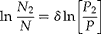
Therefore

(8)

The value of δ is the ratio of the log of the infected host fraction (numerator) to that of the corresponding parasites (denominator).

A plot of P ₂/P as a function of N ₂/N would result in a straight line if the proportion of parasites aggregated P ₂/P was equally distributed across an entire range of N ₂/N values. In cases of wealth distribution, this straight line is the Lorenz line of equal distribution known as the egalitarian line (Lorenz, Reference Lorenz1905). The distribution pattern is represented as a concave curve below the Lorenz line. The shape of its concavity is dependent on inequality in the distribution (Sen, Reference Sen1976; Kakwani, Reference Kakwani1980). In the context of infections, the straight line represents an equal aggregation of parasites in individual hosts. However, this straight line is seldom achieved as parasites are rarely distributed equally among hosts. Instead, parasite distribution is exhibited as a concave curve. The smoothness of its concavity is dependent on differential levels of intensity of infection among infected hosts. In extreme cases of parasite aggregations, when all but one host harbours zero parasites and all parasites are concentrated in a single host, the curve exhibits discontinuity.

Equation 4 is a probabilistic equation where prevalences are related to cumulated probabilities of the negative binomial probability function. Equation 5 is a deterministic equation and both equations essentially complement each other. By determining two parameters, a comprehensive description of parasite infections is achieved, with k representing how thinly or densely infected hosts are distributed and δ the intensity of infection.

Behaviour of k and δ

In survey snapshots, parasite numbers harboured by individual hosts, and hence the proportion of hosts belonging to either group A or B, or both, can vary with or without change in the mean intensity of infection. This is the dispersion aspect of infection. On the other hand, the proportion of hosts in A or B may not change but parasite burdens may vary. This is the consequence of aggregation. These scenarios involving both host and parasite perspectives can be found in snapshot surveys taken at different locations (as a spatial function) or at different times (as a temporal function).

In typical cases, if the intensity of parasites is high in a small proportion of hosts, k changes very slowly. Such variation is not sufficiently significant to reflect the higher degrees of aggregation and this insensitivity of k is well recognized by many researchers, including May and Anderson (Anderson & May, Reference Anderson and May1978; May & Anderson, Reference May and Anderson1978). Significant theoretical advantages are provided by the conventional binomial model and it has been widely applied to parasite distribution studies. However, the k index in the conventional model, which measures parasite dispersion in infected hosts in the entire host community, remains invariant under thinning (Pielou, Reference Pielou1977). Aggregation is incorporated into these models because of the need to account for non-random thinning, which is a consequence of density-dependent processes. Thus the models contain an inherent contradiction as they assume that the degree of aggregation remains constant (Smith et al., Reference Smith, Basanez, Dietz, Gemmell, Grenfell, Gulland, Hudson, Kennedy, Lloyd, Medley, Nassel, Randolph, Roberts, Shaw, Woolhouse, Grenfell and Dobson1991) despite the dynamics of population processes, which, in turn, influence the number of parasites in each host in a random manner.

The re-formulated NBD has been introduced to address these criticisms. By incrementally shifting the threshold of infection, the proportion of hosts in groups A and B are changed. The proportion of hosts is increased in A and decreased in B, the corresponding k values are calculated by applying Equation 4. Thus a set of k measures are evaluated at discrete levels of infection. Equally, the parasite aggregation index δ is evaluated at each threshold. By shifting the threshold systematically, effectively the host population is stratified. The resultant k-measure becomes a variable quantity as a function of prevalence and no longer remains invariant. Similarly, the intensity of infection in the corresponding host proportions at each threshold is determined by applying Equation 5. As the threshold increases, the proportion of hosts with highly aggregated infections is narrowed down. The stratification leads to the ranking of k and δ as a function of p _i>i*. The model may be extended for risk assessment in a host community, in terms of measures of dispersion of infected hosts, together with their intensities of infection (aggregation).

In wild host populations, typically the range in the value of k is 0 ≤ k ≤ 1.0, where parasites are aggregated in a small number of hosts, resulting in a low fraction (Anderson, Reference Anderson and Cox1993) of highly infected host population (severe contagion). The parameter k exhibits less variation with changes in the mean intensity m, and this variation in k is most pronounced when the proportion of infected hosts is in the region of 15% or less.

Taking a typical example of overdispersion, values of k lie on a plateau as the overall mean intensity changes between 10 and 100 (Anderson & May, Reference Anderson and May1991). The k parameter is very insensitive, especially when a large proportion of parasites aggregate and consequently the true amplitude of an aggregated dispersion is masked. But the application of inequality provides a measure of aggregation through δ. In the present study this approach using the ADD model is applied to the occurrence of the trichostrongylid nematode Heligmosomoides polygyrus in small and large samples of the wood mouse Apodemus sylvaticus collected from a woodland site in Surrey, southern England (Abu-Madi et al., Reference Abu-Madi, Behnke, Lewis and Gilbert2000; Pal & Lewis, Reference Pal and Lewis2004). Using data on H. polygyrus infections in a sample of 20 and of 242 hosts, a set of simulated data are prepared by varying the proportion of hosts above threshold levels (keeping m constant), and also varying the mean intensity.

Small sample of mice (Pal & Lewis, 2004)

This sample comprises 20 mice infected with the trichostrongylid nematode Heligmosomoides polygyrus (Hp) from a woodland site in Surrey. From a total population of 320 Hp and a mean intensity of infection of 16.00, the results are presented in ascending order of (a) hosts and (b) parasites (table 1).

Table 1

Results of 20 mice infected with Heligmosomoides polygyrus presented in ascending order of (a) hosts and (b) parasites.

It should be noted that all 20 mice are infected with a prevalence p = 1 and 1 − p = 0, and therefore k = ∞. However, for practical purposes, numerical calculations are performed by assigning p = 0.99 and 1 − p = 0.01.

Variation in k and δ at discrete levels of threshold i*

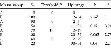
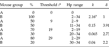
Variations in k and δ are evaluated as groups of mice are infected with H. polygyrus (Hp) above discrete threshold levels (i* = 0, 9, 19 and 29). With these changes in i* the proportion of mice in groups A and B change but the overall mean intensity remains unchanged (table 2). The conventional threshold is set at i* = 0.

Table 2

Variation in the values of k and δ as the proportion (%) of mouse groups A and B infected with Heligmosomoides polygyrus (Hp) changes at four discrete demarcation threshold i* levels, including the conventional level at 0.

^aFor the purposes of numerical calculation, proportions of hosts in groups A and B are taken as 1% and 99.0%, respectively.

k and δ as functions of threshold i* across the full range of infection levels

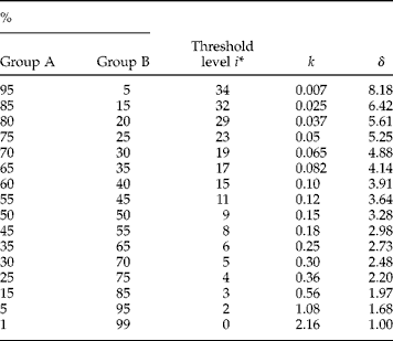
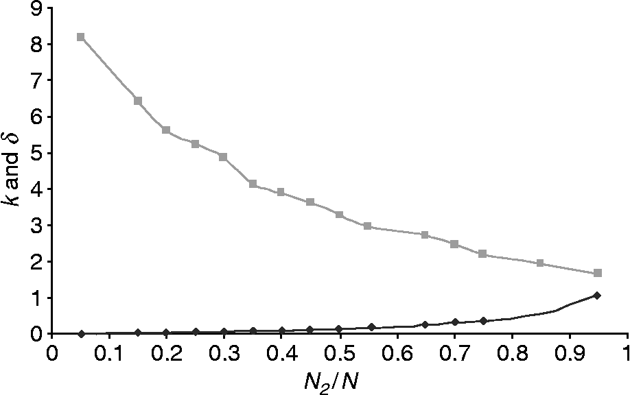
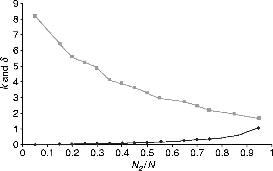
The proportion of infected mice in groups A and B will vary by systematically incrementing the threshold i*, through the full range of H. polygyrus infection levels. Corresponding k and δ indices are calculated at each step and this provides k and δ as a function of N ₂/N, the host proportion in B. The range of H. polygyrus is not included (table 3). Values of k and δ are calculated as a function of N ₂/N using Equations 6 and 7b, respectively, at relevant i* levels, showing the complementary nature of both indices (fig. 1). It is seen that k increases and δ decreases as a function of N ₂/N. Also k is not invariant across the full range of infection levels as determined by the conventional NBD. Starting with low values of N ₂/N when most parasites aggregate among a few hosts, δ is high and then declines as N ₂/N increases. The k index, on the other hand, commences at a very low level with a low N ₂/N value, which increases gradually. The insensitivity of k is shown as a very slow increase at low prevalence values. On the other hand, δ is high at low prevalences followed by a gradual decline at higher prevalences.

Table 3

Variation in the values of k and δ as the proportion (%) of mouse groups A and B infected with Heligmosomoides polygyrus (Hp) changes with the threshold level i*.

Fig. 1

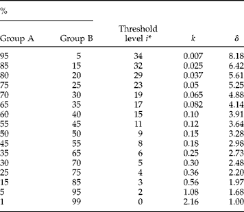
Variation in the values of k (♦)and δ () as the proportion (%) of mice (N ₂/N) infected with Heligmosomoides polygyrus (Hp) changes with the threshold level i*.

Simulation

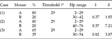
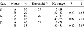
Numbers of H. polygyrus (Hp) in mouse groups A and B were varied by computer simulation, producing three cases of parasite burdens in A and B at threshold i* = 29. In case (1), parasite numbers increase in A and decrease in B, with the mean intensity remaining unchanged (m = 16.0). In case (2), parasite numbers decrease in A and increase in B, with the mean intensity unchanged (m = 16.0). In case (3), parasite numbers increase in both A and B and consequently the mean intensity changes (m = 17.55). Both k and δ are evaluated to demonstrate their sensitivity in these three cases (table 4).

Table 4

Variation in the values of k and δ as levels of infection in mouse groups A and B infected with Heligmosomoides polygyrus (Hp) change at a threshold level i*=29, using three simulated cases: note that the proportion (%) of mice infected changes with the levels of infection in case (3).

Large sample of mice (after Abu-Madi et al., Reference Abu-Madi, Behnke, Lewis and Gilbert2000)

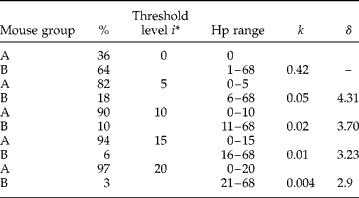
From a total of 242 mice, the population of 1067 H. polygyrus (Hp) is stratified into six discrete ranges and the numbers of mice infected in these ranges are as follows.

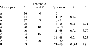
Mice are again subdivided into groups A and B with the range of Hp per group specified by threshold i*. Values of k and δ are presented at these discrete i* steps (table 5).

Table 5

Variation in the values of k and δ as the proportion (%) of mouse groups A and B infected with Heligmosomoides polygyrus (Hp) changes with the threshold level i*.

In conclusion, using the ADD model, aggregated distributions of parasites within hosts have been separated into the characteristic components of dispersion and aggregation. Corresponding k and δ values have been evaluated systematically using different thresholds of H. polygyrus infections in small and large samples of wood mouse populations. This model can be applied to the following three categories to improve our understanding of patterns of infection in host–parasite systems. First, intrinsic factors such as host age and gender are known to exhibit specific parasite aggregation, and extrinsic factors such as climate, seasonality and density-dependent processes are known to produce variation in the distribution patterns. Hence, parasite distribution in each host category is expected to conform to both negative binomial and inequality models. Second, when hosts are infected by two or more parasites possibly resulting in interactions between these parasites, patterns of their co-occurrence can be transformed by mapping the dispersion and aggregation of co-occurrences as a function of prevalence. Applying correlation analyses to the resulting k and δ indices provides a direct insight into the phenomena of parasite co-occurrences within the host population. Third, the ADD model can be used in risk analysis of infected cohorts of hosts, especially as counts of parasite numbers can be replaced by stratification of levels of infections and thresholds, as illustrated by H. polygyrus infections in the large sample of wood mice. Measures of parasite dispersion and aggregation among cohorts of hosts as functions of space and time are essential for risk assessment prior to and during an epidemic of a parasitic infection. These situations may increase as a result of global climatic changes and are therefore of concern to public health sectors worldwide. The time-dependent aggregation parameter δ reflects the outcome of the upward or downward trend in levels of infection. Further studies are therefore needed to equate the ADD model results with the basic reproductive rate of parasites, as this will be essential in analysing the risk of infection in any potential outbreaks of disease.