2.1 Flow conservation equations

We consider flows of gases in the single-phase regime, governed by the compressible Navier–Stokes equations, written in differential form as

(2.1)$$\begin{eqnarray}\displaystyle & \displaystyle \frac{\unicode[STIX]{x2202}\unicode[STIX]{x1D70C}}{\unicode[STIX]{x2202}t}+\frac{\unicode[STIX]{x2202}(\unicode[STIX]{x1D70C}u_{j})}{\unicode[STIX]{x2202}x_{j}}=0, & \displaystyle\end{eqnarray}$$

(2.2)$$\begin{eqnarray}\displaystyle & \displaystyle \frac{\unicode[STIX]{x2202}(\unicode[STIX]{x1D70C}u_{i})}{\unicode[STIX]{x2202}t}+\frac{\unicode[STIX]{x2202}(\unicode[STIX]{x1D70C}u_{i}u_{j})}{\unicode[STIX]{x2202}x_{j}}+\frac{\unicode[STIX]{x2202}p}{\unicode[STIX]{x2202}x_{i}}-\frac{\unicode[STIX]{x2202}\unicode[STIX]{x1D70F}_{ij}}{\unicode[STIX]{x2202}x_{j}}=0, & \displaystyle\end{eqnarray}$$

(2.3)$$\begin{eqnarray}\displaystyle & \displaystyle \frac{\unicode[STIX]{x2202}(\unicode[STIX]{x1D70C}E)}{\unicode[STIX]{x2202}t}+\frac{\unicode[STIX]{x2202}((\unicode[STIX]{x1D70C}E+p)u_{j})}{\unicode[STIX]{x2202}x_{j}}-\frac{\unicode[STIX]{x2202}(\unicode[STIX]{x1D70F}_{ij}u_{i})}{\unicode[STIX]{x2202}x_{j}}+\frac{\unicode[STIX]{x2202}q_{j}}{\unicode[STIX]{x2202}x_{j}}=0, & \displaystyle\end{eqnarray}$$

where $x_{i}=(x,y,z)$ are the coordinates in the streamwise, wall-normal and spanwise directions, $u_{i}=(u,v,w)$ are the corresponding velocity components, $\unicode[STIX]{x1D70C}$ is the density and $p$ is the pressure. The specific total energy is $E\equiv e+u_{j}u_{j}/2$, $e$ being the specific internal energy, and the viscous stress tensor $\unicode[STIX]{x1D70F}_{ij}$ is defined as

(2.4)$$\begin{eqnarray}\unicode[STIX]{x1D70F}_{ij}\equiv \frac{\unicode[STIX]{x1D707}}{Re}\left(\frac{\unicode[STIX]{x2202}u_{i}}{\unicode[STIX]{x2202}x_{j}}+\frac{\unicode[STIX]{x2202}u_{j}}{\unicode[STIX]{x2202}x_{i}}\right)+\frac{\unicode[STIX]{x1D706}}{Re}\frac{\unicode[STIX]{x2202}u_{k}}{\unicode[STIX]{x2202}x_{k}}\unicode[STIX]{x1D6FF}_{ij},\end{eqnarray}$$

where $\unicode[STIX]{x1D707}$ is the dynamic viscosity and $\unicode[STIX]{x1D6FF}_{ij}$ denotes the Kronecker symbol. The second viscosity is set according to Stokes’ hypothesis, $\unicode[STIX]{x1D706}=-2\unicode[STIX]{x1D707}/3$, assuming a zero bulk viscosity. This approximation is well verified for a dense gas (see appendix B of Sciacovelli et al. (Reference Sciacovelli, Cinnella and Gloerfelt2017a)). Finally, the heat flux $q_{j}$ is modelled by Fourier’s law:

(2.5)$$\begin{eqnarray}q_{j}=-\frac{\unicode[STIX]{x1D705}}{RePrEc}\frac{\unicode[STIX]{x2202}T}{\unicode[STIX]{x2202}x_{j}},\end{eqnarray}$$

where $\unicode[STIX]{x1D705}$ is the thermal conductivity. The conservation equations have been made dimensionless using the following variables:

(2.6a-d)$$\begin{eqnarray}\displaystyle \unicode[STIX]{x1D70C}=\frac{\unicode[STIX]{x1D70C}^{\ast }}{\unicode[STIX]{x1D70C}_{\infty }^{\ast }},\quad T=\frac{T^{\ast }}{T_{\infty }^{\ast }},\quad u_{i}=\frac{u_{i}^{\ast }}{u_{\infty }^{\ast }},\quad x_{i}=\frac{x_{i}^{\ast }}{L^{\ast }}, & & \displaystyle\end{eqnarray}$$

(2.6e-h)$$\begin{eqnarray}\displaystyle t=\frac{t^{\ast }u_{\infty }^{\ast }}{L^{\ast }},\quad p=\frac{p^{\ast }}{\unicode[STIX]{x1D70C}_{\infty }^{\ast }{u_{\infty }^{\ast }}^{2}},\quad \unicode[STIX]{x1D707}=\frac{\unicode[STIX]{x1D707}^{\ast }}{\unicode[STIX]{x1D707}_{\infty }^{\ast }},\quad \unicode[STIX]{x1D705}=\frac{\unicode[STIX]{x1D705}^{\ast }}{\unicode[STIX]{x1D705}_{\infty }^{\ast }}, & & \displaystyle\end{eqnarray}$$

where the superscript $^{\ast }$ indicates a dimensional quantity. The non-dimensional numbers that appear (Reynolds $Re$, Prandtl $Pr$ and Eckert $Ec$ numbers) are defined as

(2.7a-c)$$\begin{eqnarray}Re=\frac{\unicode[STIX]{x1D70C}_{\infty }^{\ast }u_{\infty }^{\ast }L^{\ast }}{\unicode[STIX]{x1D707}_{\infty }^{\ast }},\quad Pr=\frac{\unicode[STIX]{x1D707}_{\infty }^{\ast }c_{p,\infty }^{\ast }}{\unicode[STIX]{x1D705}_{\infty }^{\ast }},\quad Ec=\frac{{u_{\infty }^{\ast }}^{2}}{c_{p,\infty }^{\ast }T_{\infty }^{\ast }},\end{eqnarray}$$

where the subscript $_{\infty }$ refers to free-stream conditions, $L^{\ast }$ is a reference length and $c_{p}^{\ast }$ is the specific heat at constant pressure. We also introduce the free-stream Mach number:

(2.8)$$\begin{eqnarray}M_{\infty }=\frac{u_{\infty }^{\ast }}{c_{\infty }^{\ast }}.\end{eqnarray}$$

Note that, for an ideal gas, the Eckert number is $Ec_{\infty }=(\unicode[STIX]{x1D6FE}-1)M_{\infty }^{2}$, with $\unicode[STIX]{x1D6FE}$ the ratio of specific heats.

2.2 Equation of state and transport properties

The system is supplemented by thermal and caloric equations of state (EOS), respectively:

(2.9a,b)$$\begin{eqnarray}p=p(\unicode[STIX]{x1D70C},T)\quad \text{and}\quad e=e(\unicode[STIX]{x1D70C},T).\end{eqnarray}$$

For air, considered as a thermally and calorically perfect gas,

(2.10a,b)$$\begin{eqnarray}p^{\ast }=\unicode[STIX]{x1D70C}^{\ast }R^{\ast }T^{\ast }\quad \text{and}\quad e^{\ast }=c_{v}^{\ast }T^{\ast },\end{eqnarray}$$

where $c_{v}^{\ast }=R^{\ast }/(\unicode[STIX]{x1D6FE}-1)=\text{const.}$, $R^{\ast }={\mathcal{R}}^{\ast }/{\mathcal{M}}^{\ast }=287.06~\text{J}~\text{kg}^{-1}~\text{K}^{-1}$ (with ${\mathcal{R}}^{\ast }$ being the universal gas constant and ${\mathcal{M}}^{\ast }$ the gas molecular weight) and $\unicode[STIX]{x1D6FE}=1.4$. Sutherland’s law is used to model the viscosity $\unicode[STIX]{x1D707}$:

(2.11)$$\begin{eqnarray}\frac{\unicode[STIX]{x1D707}^{\ast }}{\unicode[STIX]{x1D707}_{ref}^{\ast }}=\left(\frac{T^{\ast }}{T_{ref}^{\ast }}\right)^{3/2}\,\frac{T_{ref}^{\ast }+S_{0}^{\ast }}{T^{\ast }+S_{0}^{\ast }},\end{eqnarray}$$

with $\unicode[STIX]{x1D707}_{ref}^{\ast }=1.716\times 10^{-5}~\text{Pa}~\text{s}$, $T_{ref}^{\ast }=273.15~\text{K}$ and $S_{0}^{\ast }=110.4~\text{K}$. A constant-Prandtl-number assumption is used to determine the thermal conductivity $\unicode[STIX]{x1D705}^{\ast }=c_{p}^{\ast }\,\unicode[STIX]{x1D707}^{\ast }/Pr$ (with $Pr=0.72$).

Table 1.

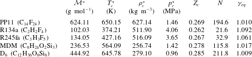
Thermodynamic properties of the selected dense gases: molecular weight (${\mathcal{M}}^{\ast }$), critical temperature ($T_{c}^{\ast }$), critical density ($\unicode[STIX]{x1D70C}_{c}^{\ast }$), critical pressure ($p_{c}^{\ast }$), critical compressibility factor ($Z_{c}=p_{c}^{\ast }/(\unicode[STIX]{x1D70C}_{c}^{\ast }R^{\ast }T_{c}^{\ast })$), molecular complexity ($N$) in terms of the number of active degrees of freedom, and equivalent ratio of ideal-gas specific heat at constant pressure and volume ($c_{p,\infty }^{\ast }(T_{c}^{\ast })/c_{v,\infty }^{\ast }(T_{c}^{\ast })$).

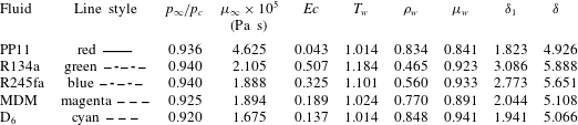
In the present study, five different dense gases are considered. Most of the results are obtained for PP11, which was used in our previous studies (Sciacovelli et al. Reference Sciacovelli, Cinnella, Content and Grasso2016, Reference Sciacovelli, Cinnella and Gloerfelt2017a,Reference Sciacovelli, Cinnella and Grassob), since it exhibits a relatively large inversion zone ($\unicode[STIX]{x1D6E4}<0$). PP11 is the commercial name of the perfluoro-perhydro-phenanthrene, which belongs to the family of fluorocarbons (see Cramer Reference Cramer1989). We have also selected two refrigerants in the family of hydrofluorocarbons, which are widely used in ORC: R134a (1,1,1,2-tetrafluoroethane) and R245fa (1,1,1,3,3-pentafluoropropane). Finally, two siloxanes are considered: a relatively light linear siloxane called MDM (octamethyltrisiloxane), used in a recent experimental apparatus (Spinelli et al. Reference Spinelli, Cammi, Conti, Gallarini, Zocca, Cozzi, Gaetani, Dossena and Guardone2019), and a relatively heavy cyclic siloxane D₆ (dodecamethylcyclohexasiloxane), which is expected to exhibit an inversion zone and is used in the FAST experimental facility at TU Delft (Mathijssen et al. Reference Mathijssen, Gallo, Casati, Nannan, Zamfirescu, Guardone and Colonna2015). Some thermodynamic properties of these gases are given in table 1. In the table we also report the number of active degrees of freedom ($N$) of the gas evaluated at its critical temperature, which is an indication of the molecular complexity of the gas and is defined as (Colonna & Guardone Reference Colonna and Guardone2006)

(2.12)$$\begin{eqnarray}N=2\frac{c_{v,\infty }^{\ast }(T_{c}^{\ast })}{R^{\ast }}\quad \text{with }c_{v,\infty }^{\ast }(T^{\ast })=\lim _{v^{\ast }\rightarrow \infty }c_{v}^{\ast }(v^{\ast },T^{\ast })\end{eqnarray}$$

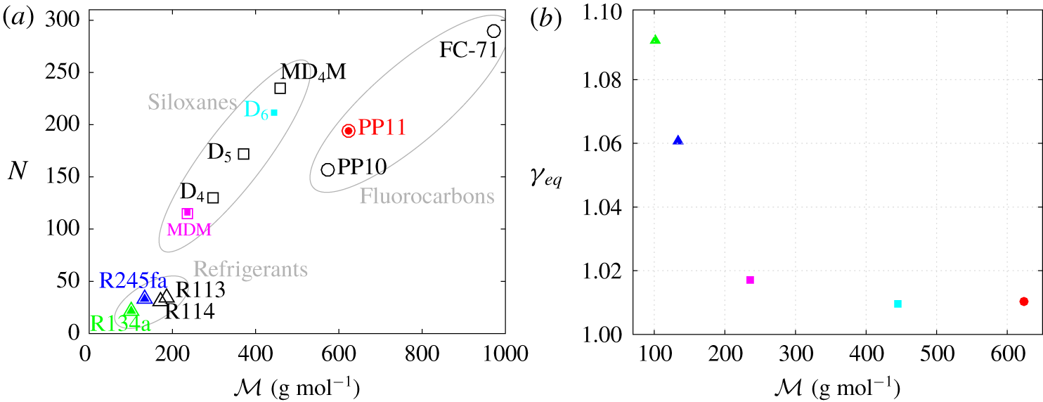
and $v^{\ast }=1/\unicode[STIX]{x1D70C}^{\ast }$ is the specific volume. The equivalent specific heat ratio is defined as $\unicode[STIX]{x1D6FE}_{eq}=1+2/N$. In figure 1, we report $N$ and $\unicode[STIX]{x1D6FE}_{eq}$ for the different families of dense gases. Figure 1 shows the dependence of the molecular complexity on the molecular weight. For the heaviest and more complex fluids, $N$ varies nearly linearly with ${\mathcal{M}}^{\ast }$. Note that the heaviest compounds considered in the study (D₆ and PP11) have roughly similar values of $N$ and $\unicode[STIX]{x1D6FE}_{eq}$, even though D₆ has a lower molecular weight than PP11.

Figure 1.

Molecular complexity (a) and equivalent specific heat ratio (b) as functions of molecular weight for the selected dense gases. Coloured solid symbols correspond to values computed in the present study, and open symbols are from Cramer (Reference Cramer1989) for fluorocarbons and from Harinck, Guardone & Colonna (Reference Harinck, Guardone and Colonna2009) for refrigerants and siloxanes.

R134a, R245fa, MDM and D₆ are modelled by means of the NIST REFPROP library (Lemmon, Huber & McLinden Reference Lemmon, Huber and McLinden2013), which contains the most accurate models available for EOS and transport properties. More specifically, the models consist of multi-parameter functional forms based on the Helmholtz free energy for the EOS, namely the models of Tillner-Roth & Baehr (Reference Tillner-Roth and Baehr1994) for R134a, Akasaka, Zhou & Lemmon (Reference Akasaka, Zhou and Lemmon2015) for R245fa, Thol et al. (Reference Thol, Dubberke, Baumhögger, Vrabec and Span2017) for MDM and Colonna, Nannan & Guardone (Reference Colonna, Nannan and Guardone2008) for D₆. These correlations are accurate in the range of ($p,v,T$) values used in the present study. The extended corresponding states models of Huber, Laesecke & Perkins (Reference Huber, Laesecke and Perkins2003) are used for transport properties of R134a, MDM and D₆. For R245fa, recent measurements and correlations for viscosity and thermal conductivity are used (Perkins, Huber & Assael Reference Perkins, Huber and Assael2016). The more validated correlation is that for R134a with reported uncertainties of the order of 5 % for the viscosity. For the other fluids, the semi-empirical relations for transport properties may suffer from greater uncertainties in the supercritical regime of interest.

For PP11, the thermal equation of state is that of Martin & Hou (Reference Martin and Hou1955), which has been chosen in several previous works for fluorocarbons (Thompson & Lambrakis Reference Thompson and Lambrakis1973; Cramer Reference Cramer1989, Reference Cramer and Kluwick1991; Guardone, Vigevano & Argrow Reference Guardone, Vigevano and Argrow2004) in the absence of more validated EOS. This equation involves five virial terms and ensures high accuracy with a minimum amount of experimental information:

(2.13)$$\begin{eqnarray}p^{\ast }=\frac{R^{\ast }T^{\ast }}{(v^{\ast }-b^{\ast })}+\mathop{\sum }_{i=2}^{5}\frac{f_{i}(T^{\ast })}{(v^{\ast }-b^{\ast })^{i}},\end{eqnarray}$$

with $b^{\ast }=v_{c}^{\ast }(1-\unicode[STIX]{x1D6FD}/Z_{c})$, $\unicode[STIX]{x1D6FD}=20.533Z_{c}-31.883Z_{c}^{2}$ and

(2.14)$$\begin{eqnarray}f_{i}(T^{\ast })=A_{i}+B_{i}T^{\ast }+C_{i}\exp (-kT^{\ast }/T_{c}^{\ast }),\end{eqnarray}$$

where $v_{c}^{\ast }$, $T_{c}^{\ast }$ and $Z_{c}$ are the critical specific volume, temperature and compressibility factor, respectively, and $k=5.475$. Here $A_{i}$, $B_{i}$ and $C_{i}$ are gas-dependent coefficients that can be expressed in terms of the critical temperature and pressure, the critical compressibility factor, the Boyle temperature (which may be expressed as a function of the critical temperature) and one point on the vapour pressure curve. The temperature dependence of the low-density specific heat is approximated by a power law:

(2.15)$$\begin{eqnarray}c_{v,\infty }^{\ast }(T^{\ast })=c_{v,\infty }^{\ast }(T_{c}^{\ast })\left(\frac{T^{\ast }}{T_{c}^{\ast }}\right)^{n},\end{eqnarray}$$

where $n=0.5776$ for PP11. The fluid viscosity and thermal conductivity are evaluated by means of the generalized laws derived by Chung et al. (Reference Chung, Ajlan, Lee and Starling1988), which contain a correction term that takes into account the strong density dependence of the transport properties in the dense-gas region. Details about the laws of Chung et al. (Reference Chung, Ajlan, Lee and Starling1988) are given in appendix A of Sciacovelli et al. (Reference Sciacovelli, Cinnella and Gloerfelt2017a).

4.1 Base flow solutions

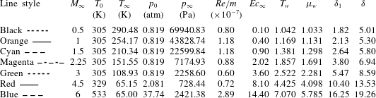
First, the influence of the Mach number on an adiabatic boundary layer is investigated for both air and PP11. The reference thermodynamic quantities for air are typical of wind tunnel conditions. For Mach numbers $M_{\infty }=0.5$ to 3, the stagnation temperature and pressure values are $T_{0}=305~\text{K}$ and $p_{0}=0.819~\text{atm}$, respectively; at $M_{\infty }=6$, we take $T_{0}=533~\text{K}$ and $p_{0}=37.74~\text{atm}$. These conditions have been used in previous stability studies (Wazzan, Taghavi & Keltner Reference Wazzan, Taghavi and Keltner1984; Mack Reference Mack1984b; Reed & Balakumar Reference Reed and Balakumar1990). At $M_{\infty }=4.5$, which serves as a reference point in the present study, the conditions in the paper of Ma & Zhong (Reference Ma and Zhong2003) are used, namely $\unicode[STIX]{x1D70C}_{\infty }=0.03895~\text{kg}~\text{m}^{-3}$ and $T_{\infty }=65.15~\text{K}$. For air, the Prandtl number is set equal to 0.72, as in Ma & Zhong (Reference Ma and Zhong2003). The values for stagnation and static quantities are summarized in table 2.

Table 2.

Influence of Mach number for a perfect gas at $Re=2000$: boundary-layer properties from similarity solution.

Table 3.

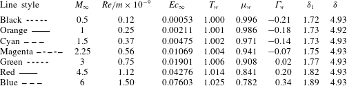
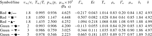
Influence of Mach number for a dense gas at $Re=2000$: boundary-layer properties from similarity solution.

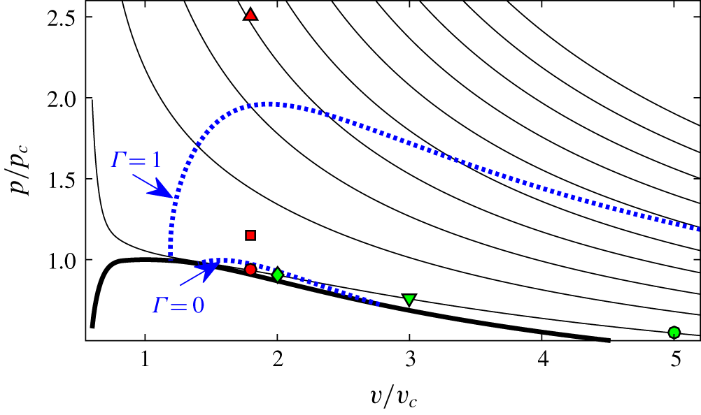
The operating point for PP11 is taken inside its inversion zone (further details are given in § 5, where the influence of the operating point is discussed). The free-stream conditions are fixed by using a specific volume $v_{\infty }=1.8v_{c}$ and a temperature $T_{\infty }=0.995T_{c}$, yielding $\unicode[STIX]{x1D70C}_{\infty }=348.4~\text{kg}~\text{m}^{-3}$ and $T_{\infty }=646.8~\text{K}$, which correspond to a slightly supercritical wall temperature condition that avoids the occurrence of a two-phase flow. The fundamental derivative of gas dynamics is negative in the free stream ($\unicode[STIX]{x1D6E4}_{\infty }=-0.217$) and can become positive near the wall depending on the Mach number (see table 3). Such thermodynamic conditions are selected for consistency with previous DNS studies and with the aim of achieving the largest possible deviations from air, although these conditions are difficult to reproduce in an experimental facility, in particular, due to the risks of thermal decomposition of the fluid. The sensitivity of stability results to the operating conditions is discussed in § 5.1.

Figure 2.

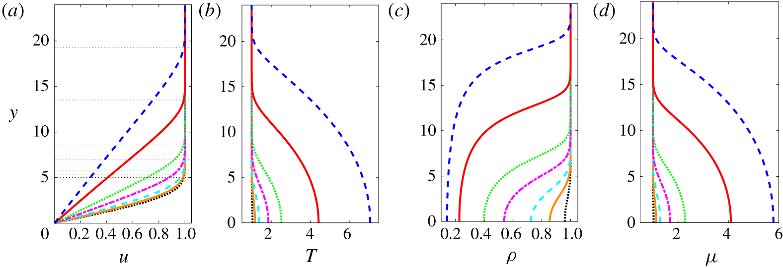
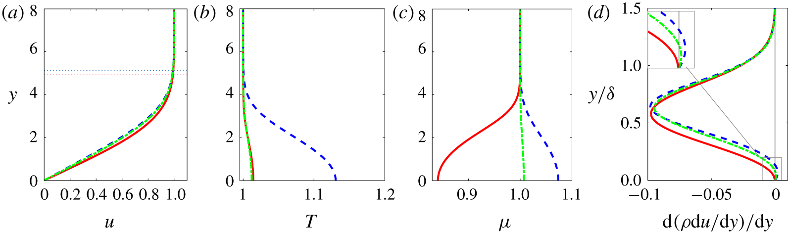
Similarity solution for air (perfect gas). Line legend as in table 2. The horizontal dotted lines in (a) mark the boundary-layer thickness $\unicode[STIX]{x1D6FF}$.

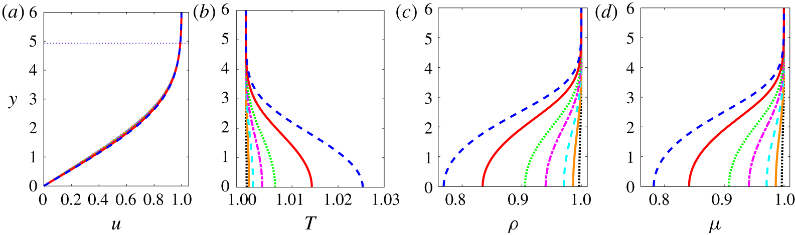
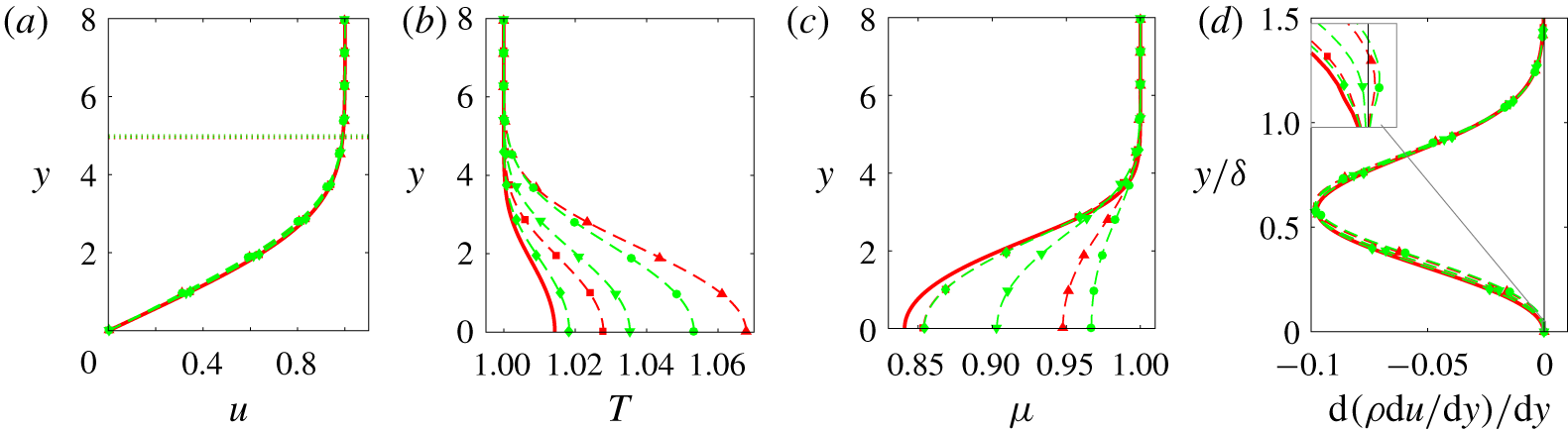
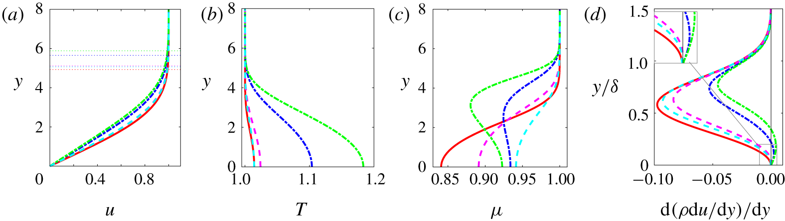
Figures 2 and 3 show the similarity solutions respectively for air and PP11 at various Mach numbers, as a function of the similarity variable $\unicode[STIX]{x1D702}_{inc}=y^{\ast }/\sqrt{(\unicode[STIX]{x1D707}_{\infty }^{\ast }x^{\ast })/(\unicode[STIX]{x1D70C}_{\infty }^{\ast }u_{\infty }^{\ast })}\equiv y$. The most striking results are the differences in the thickening of the boundary layer (figures 2a and 3a). For air, due to the increase in viscosity (figure 2d), which in turn is a direct consequence of friction heating (figure 2b), the boundary layer thickens considerably as the Mach number grows.

On the contrary, for PP11, the velocity profiles remain almost indistinguishable from the incompressible counterpart, as already observed in the case of dense-gas laminar boundary layers (Cramer et al. Reference Cramer, Whitlock and Tarkenton1996; Kluwick Reference Kluwick2004; Cinnella & Congedo Reference Cinnella and Congedo2007), and this is the result of the weaker dependence of wall thermodynamic quantities ($T$, $\unicode[STIX]{x1D70C}$ and $\unicode[STIX]{x1D707}$) on the Mach number. For example, the largest increase in wall temperature is only 2.5 % for $M_{\infty }=6$ for the dense gas, whereas a factor greater than 7 is obtained for the perfect gas. Wall values from the similarity solutions are given in tables 2 and 3, together with the non-dimensional boundary-layer thickness, $\unicode[STIX]{x1D6FF}$ (evaluated at $u=0.99$), and the displacement thickness, $\unicode[STIX]{x1D6FF}_{1}$. Furthermore, the values of the Eckert number for PP11 are two orders of magnitude less than those for air (see tables 2 and 3), in accordance with the asymptotic analysis of Kluwick (Reference Kluwick2004). It is also interesting to recall that in dense gas the viscosity has an opposite evolution compared to the perfect one and is closely correlated with the density (figures 3c and 3d).

Figure 3.

Similarity solution for PP11 (dense gas). Line legend as in table 3. The horizontal dotted lines in (a) mark the boundary-layer thickness $\unicode[STIX]{x1D6FF}$.

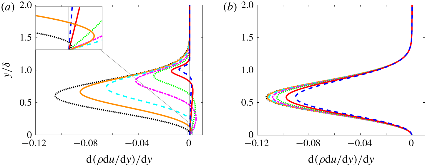
An important property of the base flow is the presence of a generalized inflection point, $\text{d}(\unicode[STIX]{x1D70C}\,\text{d}u/\text{d}y)/\text{d}y=0$. Lees & Lin (Reference Lees and Lin1946) demonstrated that it gives a necessary condition for a compressible boundary-layer flow to be inviscidly unstable. Ren et al. (Reference Ren, Marxen and Pecnik2019b) showed that a similar criterion is applicable for non-ideal gases. The distributions of $\text{d}(\unicode[STIX]{x1D70C}\,\text{d}u/\text{d}y)/\text{d}y$ with $y/\unicode[STIX]{x1D6FF}$ are plotted in figure 4. The outward movement of the generalized inflection point with increasing $M_{\infty }$ is apparent in figure 4(a) for the perfect gas. On the contrary, no inflection point is observed for PP11 at this operating point, which indicates that an inviscid mechanism would not exist for the dense gas and the first mode should remain viscous in nature.

Figure 4.

Distribution of generalized derivatives $\text{d}(\unicode[STIX]{x1D70C}\,\text{d}u/\text{d}y)/\text{d}y$ for perfect-gas (a) and dense-gas (b) boundary layers. Line legends as in tables 2 and 3.

Figure 5.

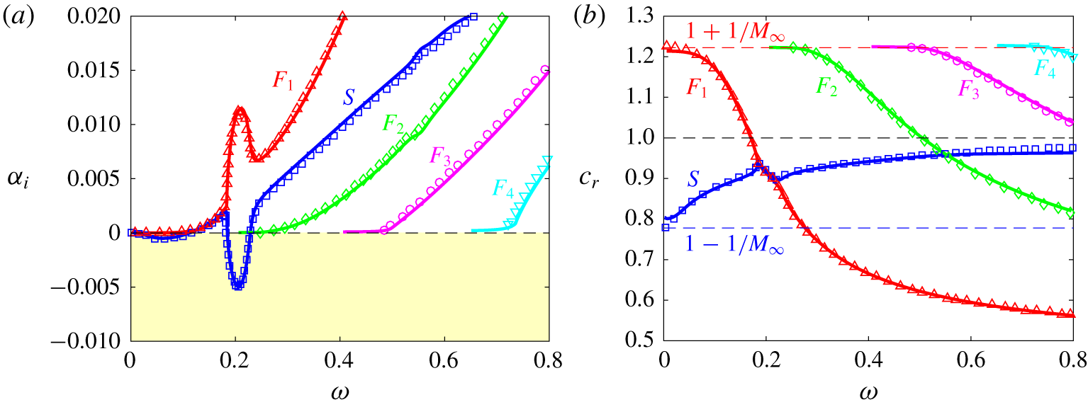
The LST for a perfect gas at $M=4.5$ and $Re=2000$: growth rate (a) and phase speed (b). Present results (solid lines) are compared with results of Ma & Zhong (Reference Ma and Zhong2003) (symbols) for the slow mode $S$ (blue ——, blue ▫) and the fast modes $F_{1}$ (red ——, red ▵), $F_{2}$ (green ——, green ♢), $F_{3}$ (magenta ——, magenta ○) and $F_{4}$ (cyan ——, cyan ▿).

Figure 6.

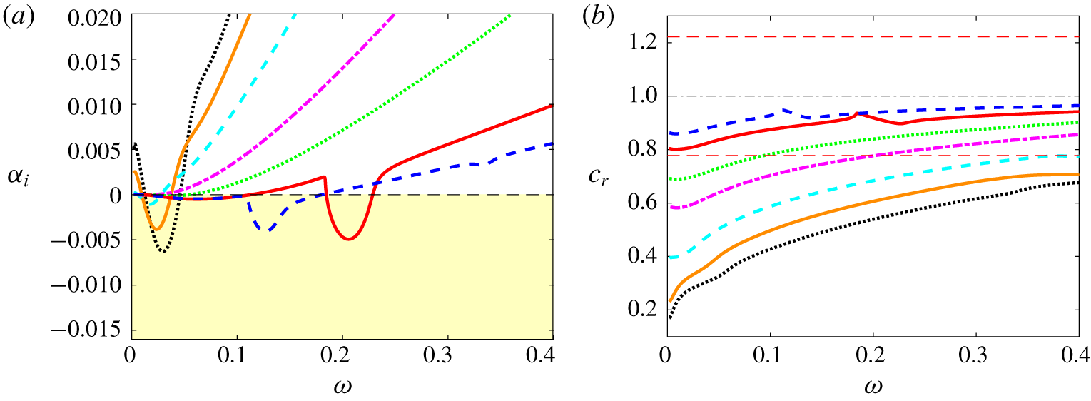
Influence of Mach number for perfect gas at $Re=2000$: growth rate (a) and phase speed (b). Line legend as in table 2. In (b), the horizontal dash-dotted line marks the location of the vorticity/entropy branch and the dashed lines above and below indicate the fast and slow acoustic branches at $M_{\infty }=4.5$, respectively.

4.2 Validation and terminology

For the purpose of validation and to introduce the terminology used in the later sections, we briefly present the LST results of the $M_{\infty }=4.5$ and $Re=2000$ case that has been thoroughly studied by Ma & Zhong (Reference Ma and Zhong2003). The computed growth rate and phase speed (continuous lines in figure 5) are in very good agreement with the results reported by Ma & Zhong (Reference Ma and Zhong2003) (symbols). For the terminology, we follow Fedorov & Tumin (Reference Fedorov and Tumin2011) and Ma & Zhong (Reference Ma and Zhong2003). A slow mode $S$ (respectively, a fast mode $F$) is a mode having a phase speed equal to the one of the slow (respectively, fast) acoustic mode at zero frequency, namely $c_{\unicode[STIX]{x1D711}}=1-1/M_{\infty }$ (respectively, $c_{\unicode[STIX]{x1D711}}=1+1/M_{\infty }$). In figure 5, a first region of instability, with a maximum growth rate of approximately -5 × 10^-4 for $\unicode[STIX]{x1D714}\approx 0.06$, corresponds to the first mode (extension of the TS mode). A second region, with a negative peak at $\unicode[STIX]{x1D714}\approx 0.2$ and a growth rate 10 times greater, is associated with the second mode (or Mack mode I). Both are associated with the slow mode $S$, meaning that they arise from the same eigenvalue. This mode remains subsonic and its phase velocity increases with $\unicode[STIX]{x1D714}$ (figure 5b). The fast mode $F_{1}$ has a decreasing phase speed; it first crosses the vorticity/entropy branch, characterized by a unitary phase speed, then crosses the slow mode, leading to the synchronization of the modes ($\unicode[STIX]{x1D6FC}_{r,S}=\unicode[STIX]{x1D6FC}_{r,F}$) as described by Fedorov & Khokhlov (Reference Fedorov and Khokhlov2001) and Fedorov & Tumin (Reference Fedorov and Tumin2011). During this phase, the slow mode is strongly destabilized and the fast mode is conversely stabilized. This leads to the emergence of the Mack mode, which is qualified as an acoustic mode since trapped acoustic waves are reflected between the wall and the sonic line $\widetilde{M}=-1$, where $\widetilde{M}=(u-c_{\unicode[STIX]{x1D711}})/a$ is the relative Mach number ($a$ being the sound speed). Higher-order Mack (acoustic) modes are stable and would correspond to the synchronization with the fast modes labelled $F_{2}$, $F_{3}$ and $F_{4}$ in figure 5.

4.3 Influence of the Mach number on LST

LST calculations at $Re=2000$ for 2-D waves ($\unicode[STIX]{x1D6FD}=0$) are shown in figures 6 and 7 for the various conditions given in tables 2 and 3, respectively. First, for air, only unstable modes pertaining to the mode $S$ are found and are the only ones reported in figure 6. For $M_{\infty }$ up to 3, a single unstable region is found in the low-frequency band relevant to the first-mode instability. At $M_{\infty }=0.5$, the viscous TS mode is close to what is expected in the incompressible limit. As $M_{\infty }$ is increased up to 2.25, the viscous mode is substantially stabilized and the frequency of maximum amplification diminishes. At $M_{\infty }=3$, an inversion in the behaviour occurs due to the influence of the generalized inflection point, namely the frequency of the most unstable mode rises slightly and its amplification rate starts increasing. The growth rate remains nonetheless more than one order of magnitude smaller than in the incompressible regime. The $M_{\infty }=4.5$ and $M_{\infty }=6$ cases both exhibit low-frequency instability of the first mode and instability of the second mode in a higher frequency band. At $M_{\infty }=6$, both the frequency and growth rate are reduced for the second mode with respect to $M_{\infty }=4.5$, and a higher stable mode (third mode or Mack’s mode II) starts emerging at $\unicode[STIX]{x1D714}\approx 0.34$. The phase speed (reported in figure 6b) increases with both $M_{\infty }$ and $\unicode[STIX]{x1D714}$ and it exhibits the slow-mode features within the limits of the acoustic ($c_{r}=1-1/M_{\infty }$) and vorticity/entropy ($c_{r}=1$) branches. The changes of slope in the frequency band [0.18–0.23] and [0.11–0.14] correspond to the synchronization with the fast mode (not reported in figure 6b) at $M_{\infty }=4.5$ and $M_{\infty }=6$, respectively.

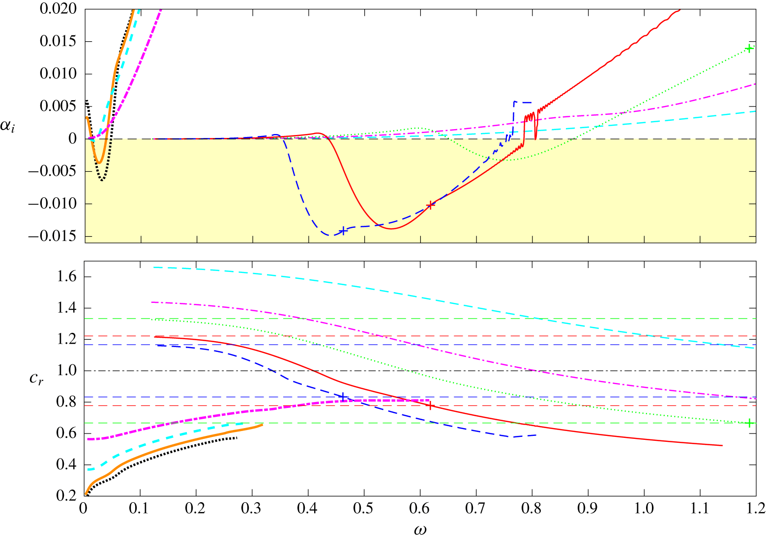
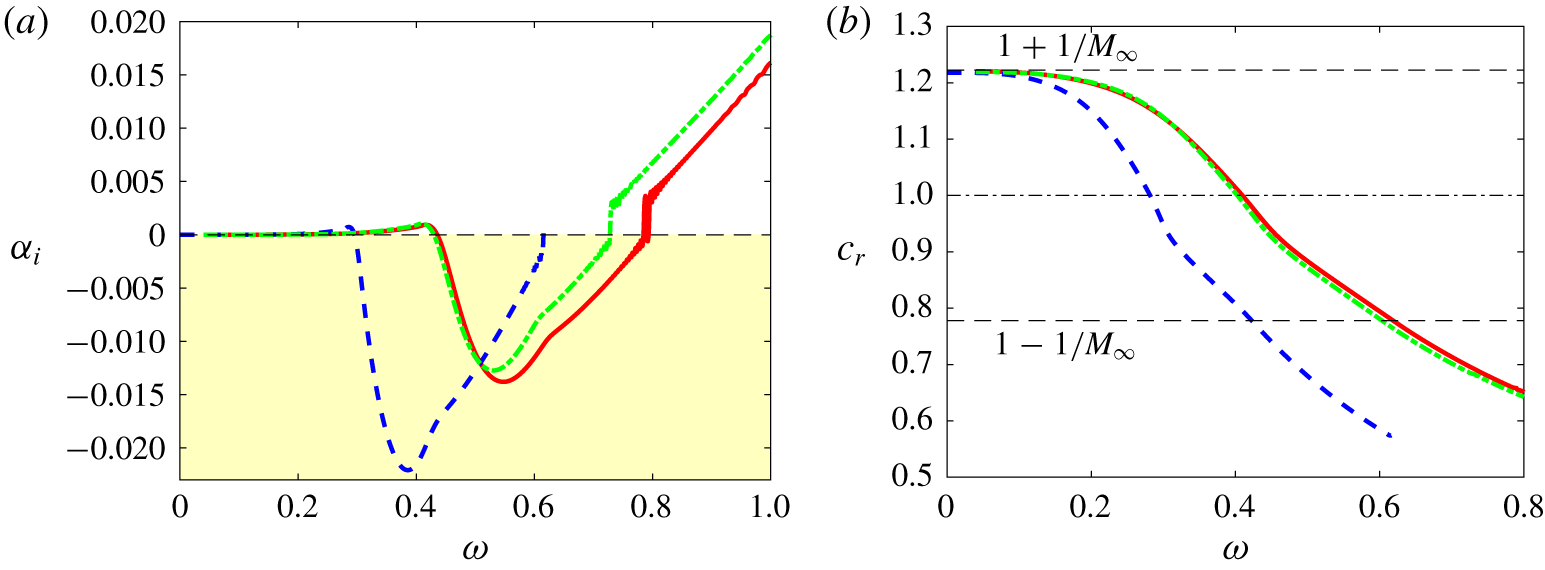
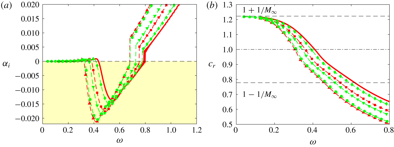
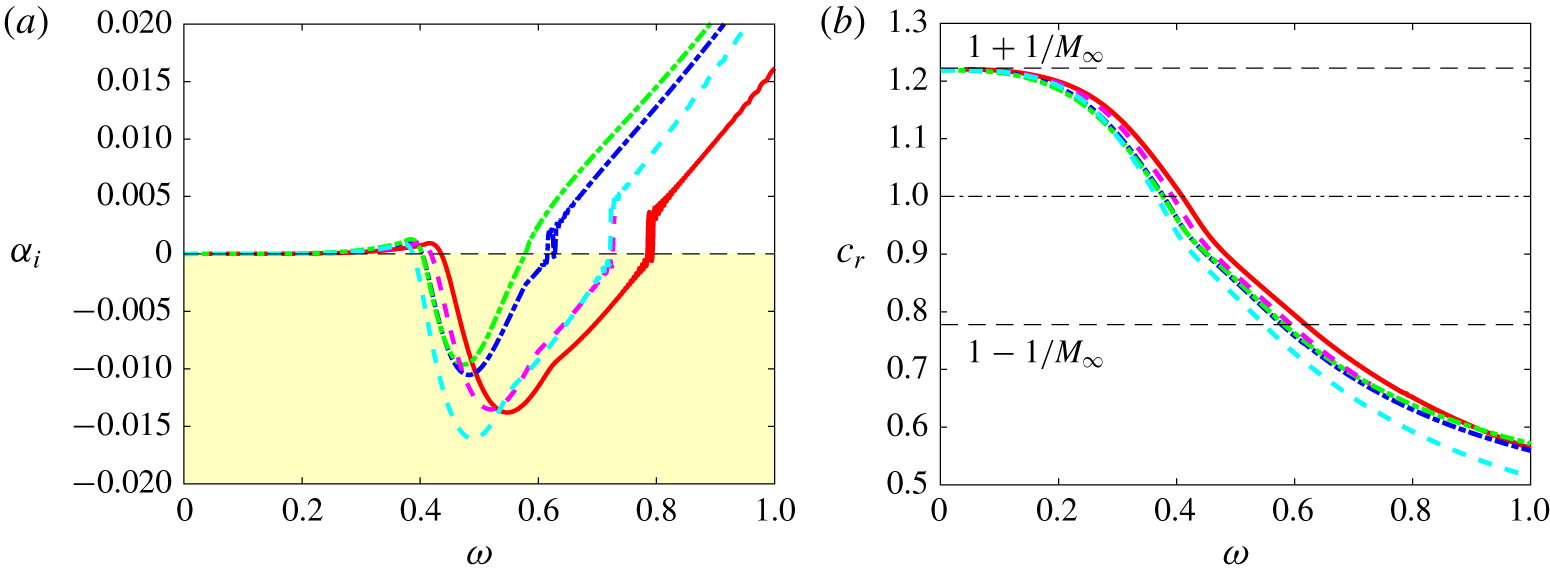
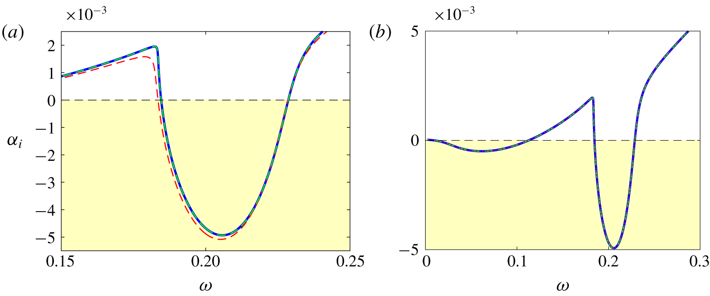
The results for the dense gas are reported in figure 7. It is interesting to observe that the unstable slow mode emerging for $0.5<M_{\infty }<1.5$ has a very similar behaviour to the perfect-gas case (see also figures 8a and 9a, where a close-up view of the growth rate is provided). This mode then undergoes strong stabilization due to the compressibility effects and the suppression of the generalized inflection point (see figure 4b). The first mode is stable for 2-D waves at $M_{\infty }=2.25$, and the mode $S$ is therefore not plotted for higher Mach numbers. A new unstable region arises for $M_{\infty }>2.25$ in a significantly higher frequency band and comes from destabilization of the fast mode $F$ (plotted with thin lines for $1.5<M_{\infty }<6$). Its maximum amplification increases with $M_{\infty }$ and the peak frequency shifts towards lower values ($\unicode[STIX]{x1D714}_{peak}=0.75$, 0.55, 0.44 for $M_{\infty }=3$, 4.5, 6). At $M_{\infty }=4.5$ and 6, the amplification curves exhibit a kink (indicated by a + symbol in figure 7), at which the decreasing phase speed reaches the value $c_{r}=1-1/M_{\infty }$, meaning that the wave travels supersonically relative to the free stream. These features are typical of the so-called supersonic mode (Bitter & Shepherd Reference Bitter and Shepherd2015; Mortensen Reference Mortensen2018; Knisely & Zhong Reference Knisely and Zhong2019a). It is worth pointing out that this mode emerges in a frequency range well above the slow-mode one (which is not the case for the first and second perfect-gas modes). Discontinuities and oscillations are visible as the mode becomes stable; their origin is discussed later in relation to figure 10.

Figure 7.

Influence of Mach number for dense gas PP11 at $Re=2000$: growth rate (a) and phase speed (b). Line legend as in table 3. In (b), the horizontal dash-dotted line marks the location of the vorticity/entropy branch and the dashed lines above and below indicate the fast and slow acoustic branches, respectively, at $M_{\infty }=3$, 4.5 and 6. For high Mach numbers, a + sign indicates the location where $c_{r}=1-1/M_{\infty }$.

Figure 8.

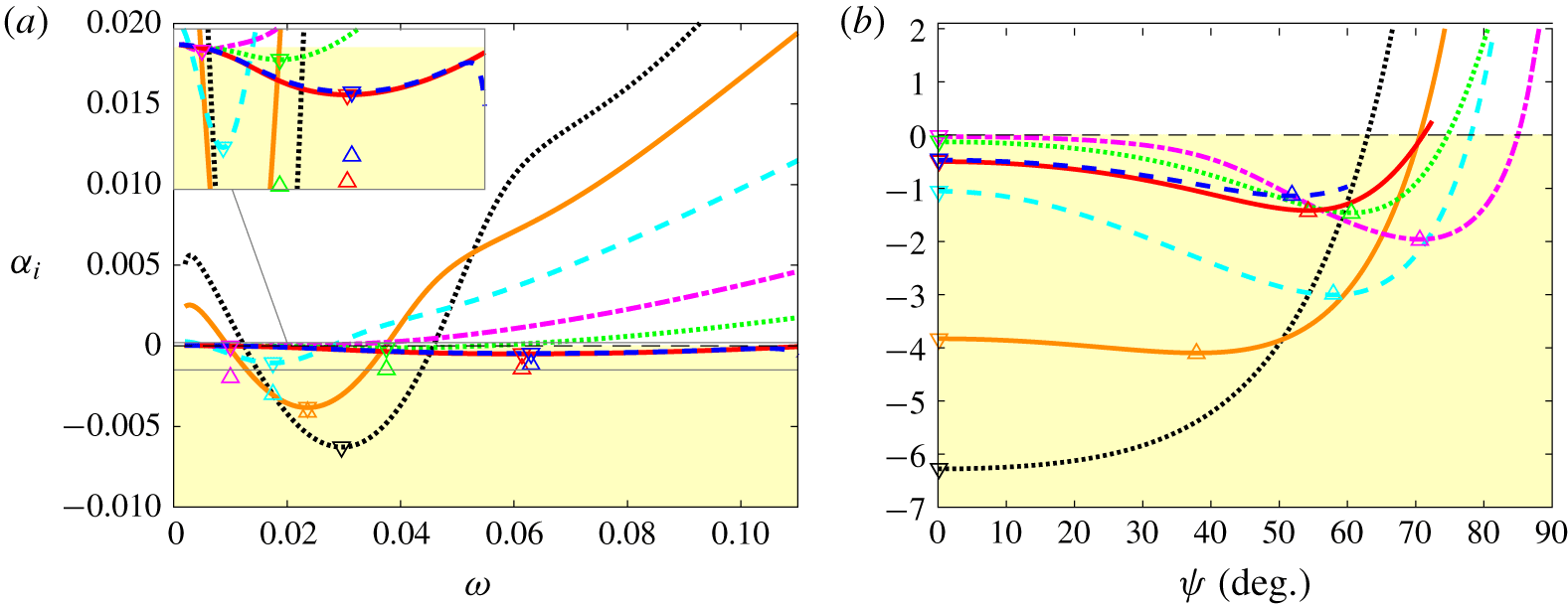
Influence of Mach number for a perfect gas at $Re=2000$: growth rate of first mode as a function of non-dimensional frequency $\unicode[STIX]{x1D714}$ for $\unicode[STIX]{x1D6F9}=0$ (a) and as a function of wave angle $\unicode[STIX]{x1D6F9}$ at the frequency of maximal 2-D growth rate (b). Here $\unicode[STIX]{x1D714}=0.0296$ for $M_{\infty }=0.5$; $\unicode[STIX]{x1D714}=0.0236$ for $M_{\infty }=1$; $\unicode[STIX]{x1D714}=0.0175$ for $M_{\infty }=1.5$; $\unicode[STIX]{x1D714}=0.01$ for $M_{\infty }=2.25$; $\unicode[STIX]{x1D714}=0.0375$ for $M_{\infty }=3$; $\unicode[STIX]{x1D714}=0.0614$ for $M_{\infty }=4.5$; and $\unicode[STIX]{x1D714}=0.0630$ for $M_{\infty }=6$. Line legend as in table 2. Symbols ▿ mark the most unstable 2-D modes, if one exists, and ▵ the most unstable 3-D waves, if one exists.

Figure 9.

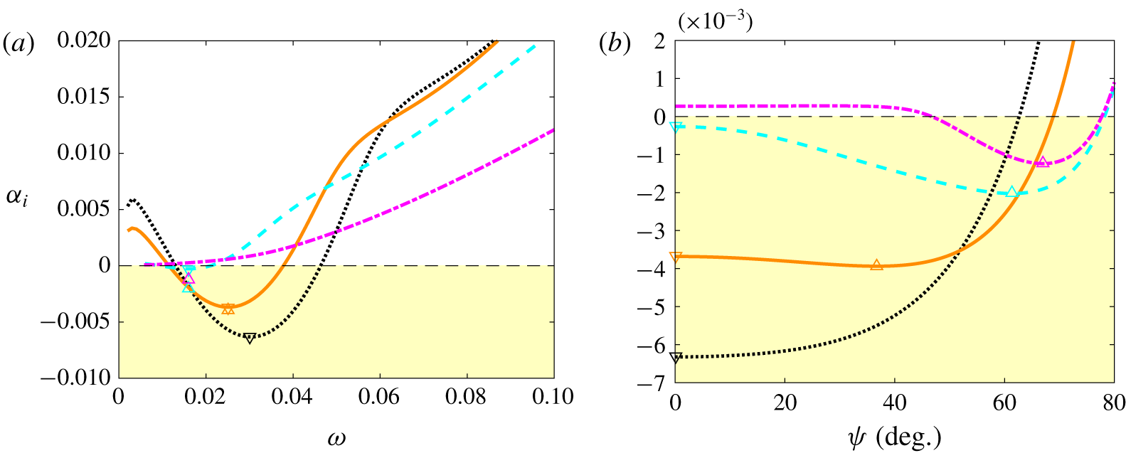
Influence of Mach number for a dense gas at $Re=2000$: growth rate of first mode as a function of non-dimensional frequency $\unicode[STIX]{x1D714}$ for $\unicode[STIX]{x1D6F9}=0$ (a) and as a function of wave angle $\unicode[STIX]{x1D6F9}$ at the frequency of maximal 2-D growth rate (b). Here $\unicode[STIX]{x1D714}=0.03$ for $M_{\infty }=0.5$; $\unicode[STIX]{x1D714}=0.025$ for $M_{\infty }=1$; $\unicode[STIX]{x1D714}$=0.016 for $M_{\infty }=1.5$; and $\unicode[STIX]{x1D714}=0.016$ for $M_{\infty }=2.25$. Line legend as in table 3. Symbols ▿ mark the most unstable 2-D modes, if one exists, and ▵ the most unstable 3-D waves, if one exists.

We now discuss in more detail the characteristics of the first mode. In the compressible regime, it is well known that there is a preference for ‘more subsonic’ skewed waves (Dunn & Lin Reference Dunn and Lin1955), i.e. 3-D waves with non-zero spanwise wavenumber $\unicode[STIX]{x1D6FD}=\unicode[STIX]{x1D6FC}_{r}\tan \unicode[STIX]{x1D6F9}$ ($\unicode[STIX]{x1D6F9}$ being the wave angle). Figures 8 and 9 show close-up views of the growth rate in the low-frequency range and its evolution with $\unicode[STIX]{x1D6F9}$ at the peak frequency for both perfect gas and dense gas at various Mach numbers. At $M_{\infty }=0.5$ and 1, the mode exhibits a similar behaviour in terms of amplification rate and frequency range for air and PP11. The 2-D wave is still the most unstable at the lowest Mach number, whereas the maximum amplifications arise at $\unicode[STIX]{x1D6F9}=37.8^{\circ }$ for air and at $\unicode[STIX]{x1D6F9}=36.8^{\circ }$ for PP11 at $M_{\infty }=1$ (with values close to that of the 2-D waves). At $M_{\infty }=1.5$, the 2-D wave is significantly stabilized by compressibility and a highly skewed wave is promoted at $\unicode[STIX]{x1D6F9}=58^{\circ }$ for air and at $\unicode[STIX]{x1D6F9}=61.4^{\circ }$ for PP11. The behaviour of the dense gas departs from that of a perfect gas at $M_{\infty }=2.25$. For air, the mode is weakly unstable in two dimensions and is substantially amplified for highly skewed waves ($\unicode[STIX]{x1D6F9}_{max}\approx 70.6^{\circ }$). As the Mach number is further increased, the inviscid mechanism becomes relevant and the rise in the peak frequency is accompanied by a slight decrease of the wave angle ($\unicode[STIX]{x1D6F9}_{max}=60.6^{\circ }$, 54. 2^° and 51. 8^° for $M_{\infty }=3$, 4.5 and 6, respectively). For PP11 at $M_{\infty }=2.25$, the 2-D wave is stable and an unstable 3-D wave is found to occur for $\unicode[STIX]{x1D714}=0.016$ and $\unicode[STIX]{x1D6F9}=67^{\circ }$. No unstable 3-D waves have been found at $M_{\infty }=3$ and higher.

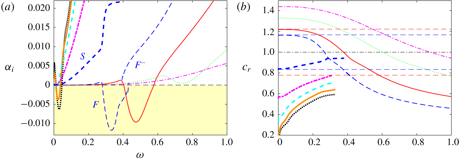
The supersonic mode that emerges in the dense-gas case is most unstable for 2-D non-skewed waves, similar to the Mack modes. We therefore focus on the 2-D case at $M_{\infty }=4.5$ and $Re=2000$. Figure 10 shows the slow mode $S$ and the two first fast modes $F_{1}$ and $F_{2}$. The mode $S$ is stable and rapidly damped as the frequency increases. 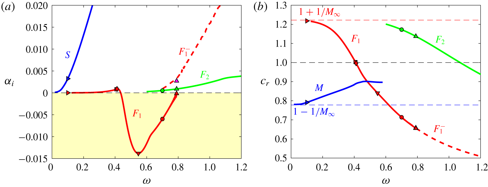The change of slope of its phase speed for frequencies at which the supersonic mode becomes unstable (figure 10b) is an indication of the synchronization phenomenon with the fast mode $F_{1}$ (Fedorov & Tumin Reference Fedorov and Tumin2011). The latter becomes most unstable at $\unicode[STIX]{x1D714}\approx 0.55$, which is significantly higher than the Mack mode ($\unicode[STIX]{x1D714}\approx 0.2$ in figure 5). As the mode stabilizes, peculiar results are observed, associated with the crossing of the acoustic branch. This kind of behaviour has already been found in the literature for supersonic modes in air and interpreted as the emergence of a new mode (generally referred to as $F_{1}^{-}$, for example in Bitter & Shepherd (Reference Bitter and Shepherd2015) or Knisely & Zhong (Reference Knisely and Zhong2019b)). Figure 10 also shows that mode $F_{2}$ appears at a much higher frequency than in the ideal-gas case.

Figure 10.

LST for a dense gas at $M=4.5$ and $Re=2000$: growth rate (a) and phase speed (b) of the slow mode $S$ (blue ——) and the fast modes $F_{1}$ (red ——), $F_{1}^{-}$ (red –  –  –) and $F_{2}$ (green ——). Frequencies, for which eigenvalue spectra are given in figure 11, are marked by symbols.

Figure 11.

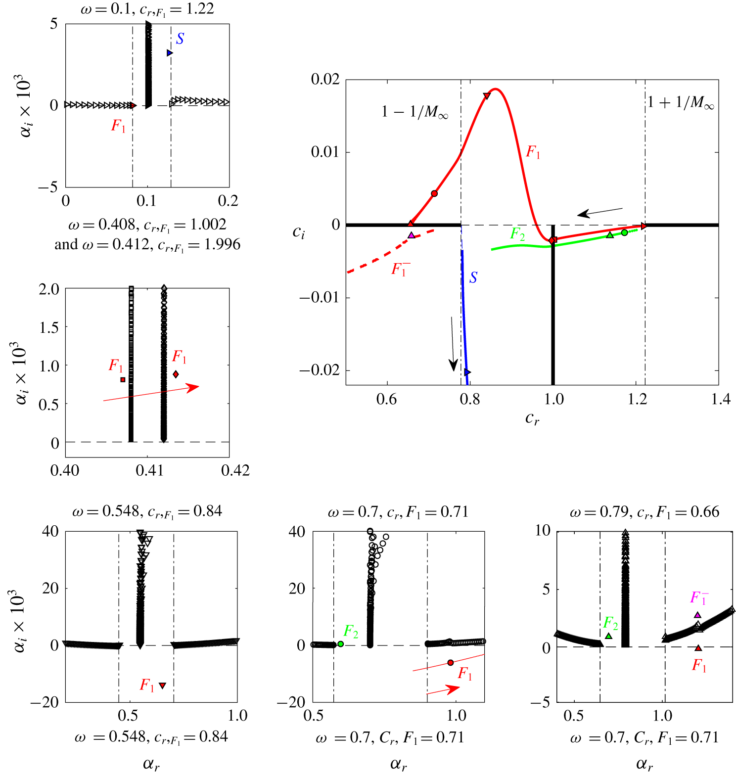
The LST for a dense gas at $M=4.5$ and $Re=2000$: map of real and imaginary parts of phase speeds in the complex plane (top right) and selected eigenvalue spectra for frequencies $\unicode[STIX]{x1D714}=0.1$ (▹), 0.408 (▫) / 0.412 (♢), 0.5475 (▿), 0.7 (○) and 0.79 (▵). Coloured filled symbols denote labelled modes, which are also plotted in the phase speed map. Arrows indicate the direction of increasing frequencies $\unicode[STIX]{x1D714}$.

To further highlight the behaviour of modes $S$, $F_{1}$ and $F_{2}$, we examine the eigenvalue spectra, reported in figure 11 for selected frequencies (corresponding to the values marked with symbols in figure 10). In figure 11, a map of the real and imaginary parts of the phase speed is also provided to help the interpretation. In the eigenvalue spectra, the two nearly horizontal lines of symbols represent the fast (on the left) and the slow (on the right) acoustic wave modes. These continuous branches originate from the phase velocities $c_{\unicode[STIX]{x1D711}}=1\pm 1/M_{\infty }$, marked by vertical dash-dotted lines (Balakumar & Malik Reference Balakumar and Malik1992). The vertical lines of symbols indicate the continuous vorticity and entropy spectra ($c_{\unicode[STIX]{x1D711}}=1$). At the lowest frequency ($\unicode[STIX]{x1D714}=0.1$), the two discrete modes $S$ and $F_{1}$ emerge from the slow and fast acoustic branches, respectively. The slow mode is already strongly damped and is seen to rapidly exit the wave-speed complex map as the frequency increases. It is therefore no longer visible in the panels corresponding to the higher-frequency spectra. A first synchronization arises as the stable fast mode crosses the vorticity/entropy waves of the continuous spectrum. It is illustrated in the second spectrum for frequencies just before (0.408) and after (0.412) the cross-over. This is accompanied by a small jump in the imaginary part $c_{i}$ (not visible at the scale of the plot), which corresponds to a substantial change of the eigenfunctions (Fedorov & Tumin Reference Fedorov and Tumin2011) and is not further discussed for the purpose of the present paper. For $\unicode[STIX]{x1D714}\approx 0.55$, the first fast mode is unstable and close to its maximum amplification rate.

As the frequency increases, the relative phase speed becomes supersonic, as it crosses the line $1-1/M_{\infty }$, at $\unicode[STIX]{x1D714}\approx 0.63$. At $\unicode[STIX]{x1D714}=0.7$, the second fast mode $F_{2}$ emerges from the fast acoustic branch and the mode $F_{1}$, located under the slow acoustic branch, has to cross this branch to stabilize. The results indicate that $F_{1}$ merges with the slow acoustic spectrum. The new discrete mode $F_{1}^{-}$ that emerges in the stable half-plane is visible in the spectrum at $\unicode[STIX]{x1D714}=0.79$ and was already observed in previous studies about the supersonic mode in air (Bitter & Shepherd Reference Bitter and Shepherd2015; Knisely & Zhong Reference Knisely and Zhong2019b). The eigenfunctions of $F_{1}$ and $F_{1}^{-}$ in the vicinity of the acoustic branch are similar within the boundary layer and are strongly oscillatory outside. Their very slow damping in the free stream makes their calculation very sensitive to numerical parameters, since an eigenvalue problem with Dirichlet free-stream boundary conditions is solved. Some authors (Bitter Reference Bitter2015; Chen, Boldini & Song Reference Chen, Boldini and Song2019) suggest to improve the calculation by using less restrictive boundary conditions in which the disturbances only remain bounded at infinity. The treatment of the acoustic branch cut in an eigenvalue problem remains tricky to interpret and an initial-value problem based on parabolized stability equations (Han, Liu & Luo Reference Han, Liu, Luo and Floryan2016) or DNS (see next section) can help to clarify this peculiar behaviour. Such calculations can be used to choose the proper solution. Although interesting from receptivity studies, the behaviour in the stable region is beyond the scope of the present investigation and will not be discussed any further.

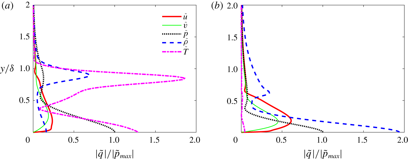
In figure 12, eigenfunctions corresponding to the most amplified supersonic mode at $M=4.5$ and $Re=2000$ (figure 12a) are compared to those obtained for the most amplified Mack mode of the perfect-gas case (figure 12b). In both cases, the eigenfunctions, normalized by the pressure amplitude at the wall, are dominated by fluctuations in thermodynamic variables, namely the temperature disturbances for the perfect-gas flow and the density disturbances for the dense-gas flow. It is worth noting that density is correlated with pressure in the dense-gas case, whereas temperature and pressure are correlated in the perfect-gas case, which is dictated by the underlying equation of state (as demonstrated in Sciacovelli et al. (Reference Sciacovelli, Cinnella and Gloerfelt2017a)). The high specific capacity of the dense gas also yields weak temperature fluctuations.

Figure 12.

Eigenfunctions normalized by the amplitude of the pressure perturbation of the most amplified waves at $M=4.5$ and $Re=2000$: perfect-gas second mode at$\unicode[STIX]{x1D714}=0.2058$ (a) and dense-gas supersonic mode at $\unicode[STIX]{x1D714}=0.5475$ (b).

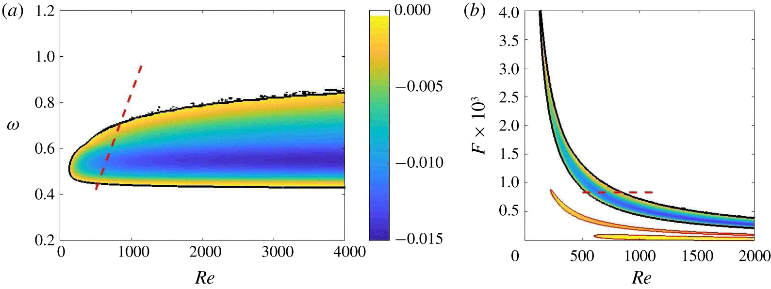
Finally, the Reynolds-number dependence of the amplified 2-D waves is shown for $M_{\infty }=4.5$ in figure 13(a). The map is bounded by the neutral curve. The oscillations visible on the upper branch are due to the crossing of the slow acoustic branch. Figure 13(a) shows a critical Reynolds number $Re\approx 200$ and, for large values of $Re$, the neutral stability points become nearly independent of $\unicode[STIX]{x1D714}$, underlining the essentially inviscid character of the supersonic mode. The qualitative characteristics of the mode do not change for $Re$ between 500 and 10 000. The comparison with neutral curves obtained for air in the $F{-}Re$ map of figure 13(b) gives an overview of the differences in frequency and amplitude of the unstable modes.

Figure 13.

Maps of 2-D amplification rate $\unicode[STIX]{x1D6FC}_{i}$ for dense gas at $M_{\infty }=4.5$ generated using the LST code: $\unicode[STIX]{x1D714}{-}Re$ (a) and $F{-}Re$ representation (b), where neutral curves of the first and second modes for a perfect gas in the same conditions are superimposed with thin red lines and the same colour scale for $\unicode[STIX]{x1D6FC}_{i}$. The black contour represents the neutral curve and the dashed red line indicates the path followed in the DNS computational domain, described in § 4.4.

4.4 Numerical simulation of the supersonic mode

In this section, we discuss some results of DNS of the supersonic mode for the dense gas PP11 at $M_{\infty }=4.5$. The aim is multi-fold: (i) to address the parallel base flow assumption of LST; (ii) to shed some light on the peculiar behaviour of the mode when crossing the acoustic branch; and (iii) to analyse the spontaneous radiation of instability waves.

Figure 14.

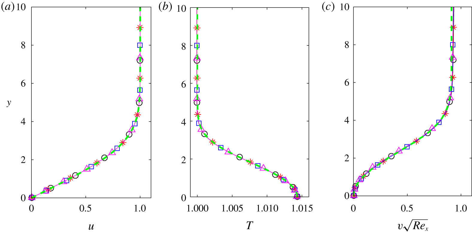
Comparison of streamwise velocity (a), temperature (b) and wall-normal velocity (c) profiles computed by the similarity solution (green –  –  –) and the DNS code at streamwise locations corresponding to $Re=825$ (black ○——), 947 (red ∗—— ), 1055 (blue ▫——) and 1152 (magenta ▵——) for a dense gas at $M_{\infty }=4.5$.

In most studies in which DNS is used to corroborate the results of LST, e.g. in Ma & Zhong (Reference Ma and Zhong2003), Egorov, Fedorov & Soudakov (Reference Egorov, Fedorov and Soudakov2006), Mayer, Von Terzi & Fasel (Reference Mayer, Von Terzi and Fasel2011), Sivasubramanian & Fasel (Reference Sivasubramanian and Fasel2015) and Knisely & Zhong (Reference Knisely and Zhong2019b), the instability wave is excited using a time-harmonic wall-normal blowing and suction boundary condition. Strong oscillations of the growth rate have been generally observed and attributed either to the coupling with continuous modes from the entropy/vorticity branch or acoustic branches, or to the synchronization between the slow and fast modes. In a first attempt, we have performed a DNS using blowing and suction (not reported for brevity), and we also found strong oscillations in the growth rate. The initial condition corresponded to $Re=500$, which is past the synchronization with the entropy/vorticity modes, and therefore the coupling with these continuous branches cannot explain the oscillations. Furthermore, the acoustic branches are sufficiently far to exclude their interaction with the excited mode, and the synchronization with the slow mode is also negligible, being highly damped. In fact, the weak shock wave, which appears as the numerical blowing and suction is introduced, is seen to act as a new waveguide trapping acoustic waves. This phenomenon was predicted by Gushchin & Fedorov (Reference Gushchin and Fedorov1989) for the leading-edge shock using Wentzel–Kramers–Brillouin (WKB) solutions of the inviscid stability equations. Following this reasoning, we argue that the shock from the blowing and suction device induces an acoustic standing wave locked at the excitation frequency and having a wavenumber different from that of the excited instability due to the different thickness of the waveguide. This wave interferes with the instability mode, which is also of acoustic nature, due to the waveguide associated with the relative sonic line. The oscillations of the growth rate may thus result from this coupling and cannot be avoided. To cope with this artefact, we then impose the instability wave directly at the inlet boundary condition using the eigenfunctions for $u$, $v$, $p$, $\unicode[STIX]{x1D70C}$ and $T$, obtained from LST. A similar strategy was also adopted by Ma & Zhong (Reference Ma and Zhong2003) to compare LST and DNS.

In the present simulation, a rectangular 2-D computational domain of 2016 × 200 points was used imposing $Re_{in}=500$. Using the Blasius length at inlet ($L_{in}^{\ast }$) as length scale, the grid has uniform streamwise resolution with $\unicode[STIX]{x0394}x\approx 1.079$, and a geometric stretching is applied in the wall-normal direction with a rate of 1.5 % and $\unicode[STIX]{x0394}y_{min}\approx 0.036$. At the inlet, the mode $F_{1}$ is imposed assuming a frequency $\unicode[STIX]{x1D714}_{forcing}=0.42$ and a non-dimensional amplitude $\unicode[STIX]{x1D700}=10^{-4}$, which ensures that the disturbance stays in the linear regime. This mode is obtained from LST with $\unicode[STIX]{x1D6FC}_{r}=0.4274$ and $\unicode[STIX]{x1D6FC}_{i}=2.93\times 10^{-3}$. The wavelength of the perturbation $\unicode[STIX]{x1D706}_{x}=2\unicode[STIX]{x03C0}/\unicode[STIX]{x1D6FC}_{r}=14.7$ is discretized by $13.6\unicode[STIX]{x0394}x$. Since the DNS results are Fourier-transformed in time to get the harmonic contribution at the forcing frequency, the time step is fixed as $\unicode[STIX]{x0394}t=(2\unicode[STIX]{x03C0}/\unicode[STIX]{x1D714}_{forcing})/600$, yielding a Courant–Friedrichs–Lewy (CFL) number of approximately 0.8.

Figure 15.

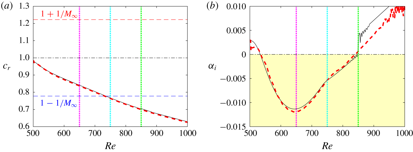
Phase speed (a) and growth rate (b) for a dense gas at $M_{\infty }=4.5$ obtained by LST (black ——) and DNS (red –  –  –). Vertical dotted lines indicate locations where eigenfunctions are compared.

First, a precursor calculation of 400 000 iterations without the excitation is run to generate the base flow. In figure 14, the precursor solution is compared with the similarity profiles at four streamwise locations. An excellent agreement is obtained, particularly for the wall-normal velocity component, which is the most sensitive quantity. The precursor DNS thus provides an accurate self-similar initial condition to investigate the instability development. The simulation is then run for 200 000 iterations with the excitation and the results are stored for the last 600 iterations, which corresponds to one period. The amplitude $A_{1}(x)$ and phase $\unicode[STIX]{x1D703}_{1}(x)$ of the complex Fourier transform at the fundamental frequency are used to compute the spatial growth rate and the streamwise wavenumber as

$$\begin{eqnarray}\unicode[STIX]{x1D6FC}_{i}=-\frac{\text{d}}{\text{d}x}[\ln (A_{1}(x))]\quad \unicode[STIX]{x1D6FC}_{r}=\frac{\text{d}}{\text{d}x}[\unicode[STIX]{x1D703}_{1}(x)].\end{eqnarray}$$

Different variables have been used to evaluate these quantities, such as the velocity components at the vertical distance of maximal amplitude or the wall pressure. Almost no differences were obtained and the results presented hereafter are based on the time Fourier transform of the wall pressure.

In figure 15, the results from DNS are compared with those from LST (following the path represented by the red dashed line in figure 13). The phase velocity of the supersonic mode is very well reproduced (figure 13a). It decreases from a value slightly below 1, i.e. after the synchronization with the entropy/vorticity branch, and reaches relative supersonic values for $Re\gtrsim 750$ (cyan vertical dotted line). The growth rate (figure 13b) compares well with LST, even though small perturbations of the DNS arise close to the inlet. The maximum growth rate computed from DNS is slightly higher, which can be attributed to non-parallel effects ignored in the LST. The trend of the LST to underpredict the amplification rate has also been observed for the second mode in a perfect gas (Ma & Zhong Reference Ma and Zhong2003). The kink in the growth rate, occurring when the disturbance becomes supersonic, is confirmed by the DNS. The peculiar behaviour observed in the LST when the supersonic mode stabilizes (at $Re\gtrsim 850$) is not found in the DNS. 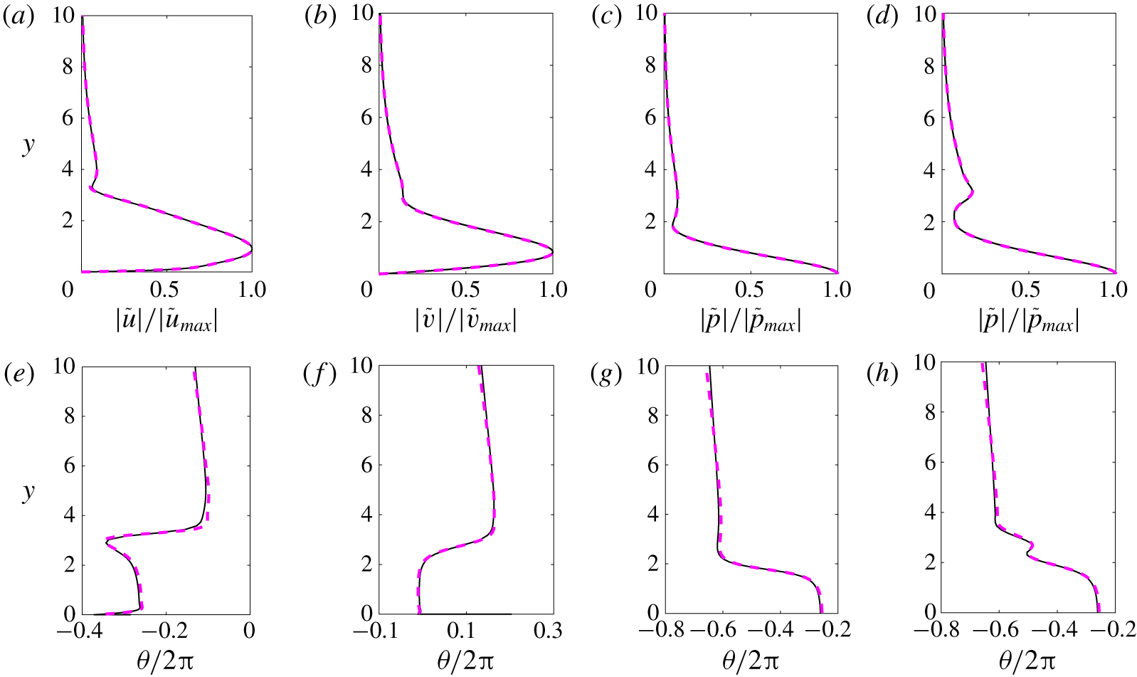Note that, as the mode evolves further stabilizing (at $Re\gtrsim 960$), some oscillations begin to appear since new perturbations develop from the background noise. In figure 16, the wall-normal amplitude and phase distributions for the streamwise velocity, wall-normal velocity, pressure and density from the DNS are compared at $Re=650$ to theoretical predictions from LST at $\unicode[STIX]{x1D714}=0.546$. The excellent agreement shows that both DNS and LST reproduce the relevant instability waves. Similar distributions and similar agreement between DNS and LST are found at higher $Re$ (not reported for brevity).

Figure 16.

Comparison of wall-normal amplitude (a–d) and phase (e–h) of the streamwise velocity, wall-normal velocity, pressure and density disturbance from DNS (magenta –  –  –) to theoretical predictions from LST (black ——) for frequency $\unicode[STIX]{x1D714}=0.546$ at $Re=650$ for a dense gas at $M_{\infty }=4.5$.

Figure 17.

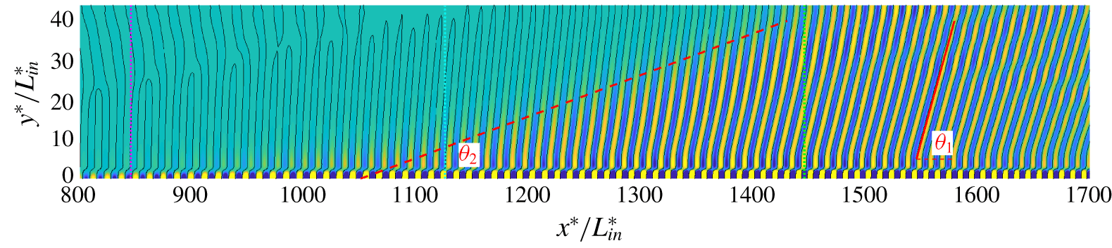
Spontaneous radiation from the supersonic mode for a dense gas at $M_{\infty }=4.5$: snapshot of the fluctuating pressure between ±2 × 10^-4 and isocontour $p^{\prime }=0$. Note that the figure is not drawn to scale.

Table 4.

Influence of EOS model for PP11 at $M_{\infty }=4.5$ with $v_{\infty }/v_{c}=1.8$ and $T_{\infty }/T_{c}=0.995$: thermodynamic conditions and boundary-layer properties from similarity solution for PFG EOS, VDW EOS and MAH EOS.

Figure 18.

Influence of EOS model on similarity solutions for PP11 at $M_{\infty }=4.5$. Line legend as in table 4.

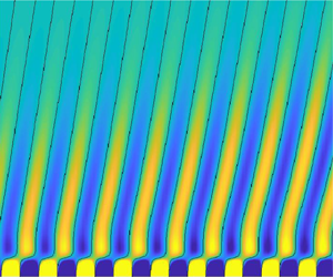
A snapshot of the fluctuating pressure field is depicted in figure 17, where the spontaneous radiation from the supersonic mode is visible. A similar behaviour has been observed by other authors (Bitter & Shepherd Reference Bitter and Shepherd2015; Chuvakhov & Fedorov Reference Chuvakhov and Fedorov2016; Salemi & Fasel Reference Salemi and Fasel2018; Knisely & Zhong Reference Knisely and Zhong2019a) for the supersonic mode in air. Above the second sonic line, $c_{\unicode[STIX]{x1D711}}=u-a$, wave fronts are radiated to the outer flow with an angle $\unicode[STIX]{x1D703}_{1}\approx 45^{\circ }$. These waves form a beam with an exterior boundary inclined at the angle $\unicode[STIX]{x1D703}_{2}\approx 6^{\circ }$ with respect to the wall, smaller than the Mach wave angle $\sin ^{-1}(1/M_{\infty })\approx 12.8^{\circ }$. The same characteristics have been observed for supersonic mode in air in Chuvakhov & Fedorov (Reference Chuvakhov and Fedorov2016) and Salemi & Fasel (Reference Salemi and Fasel2018) at Mach numbers 5 and 6, respectively.

4.5 Analysis of the supersonic mode

The features of the supersonic mode found in PP11 are similar to those of the supersonic mode observed for air at high-enthalpy conditions and a cold wall. In order to shed some light on the appropriate scaling to identify the effects associated with the dense gas, we have thus considered three different thermodynamic models, namely: the polytropic perfect-gas equation (PFG) with an equivalent specific heat ratio (as defined in § 2.2); the van der Waals equation (VDW); and the Martin and Hou equation (MAH). For the two former gas models, a temperature power law is used for the viscosity (with exponent 0.58) and a constant Prandtl number is assumed ($Pr=1.67$). The free-stream specific volume and temperature are those used in § 4.1. The thermodynamic conditions and mean flow properties are given in table 4 and figure 18. It is worth pointing out that the velocity profiles for the three models (figure 18a) show a weak thickening of the boundary layer, as indicated by the last two columns of table 4 corresponding to the displacement and 99 % thicknesses. The density variations are also similar (only wall values are reported in table 4). However, both the PFG and VDW gases exhibit a generalized inflection point close to the wall (figure 18d). The temperature increase at the wall is approximately 13 % for PFG and only 1 % for VDW and MAH (figure 18b). Another marked difference is to be noticed for the dynamic viscosity, which has a gas-like behaviour for the simplified models (due to the use of a power law). The variations across the boundary layer for VDW are nonetheless very small. The free-stream value of the fundamental derivative of gas dynamics of PFG is constant and greater than 1 ($\unicode[STIX]{x1D6E4}_{\infty }=(1+\unicode[STIX]{x1D6FE}_{eq})/2$), whereas VDW predicts a larger inversion zone than MAH (Sciacovelli et al. Reference Sciacovelli, Cinnella and Grasso2017b) and thus provides higher $\unicode[STIX]{x1D6E4}_{\infty }$ values.

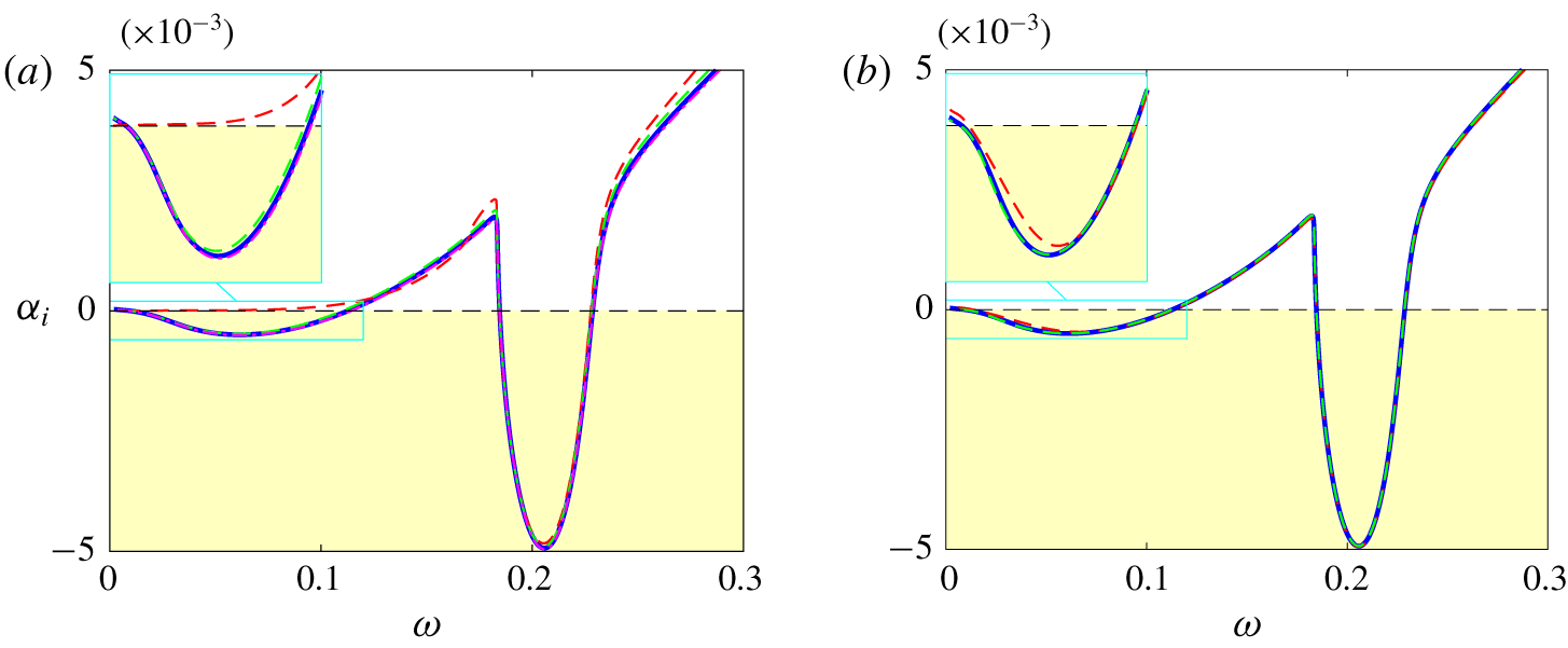
LST results for 2-D waves at $M_{\infty }=4.5$ and $Re=2000$ are shown in figure 19. The three different gas models all exhibit a supersonic mode. The growth rate and phase velocity are fairly close for VDW and MAH. The maximum amplification is greater and the frequency lower with PFG, which also yields a more rapid decay of the phase speed. The appearance of the supersonic mode by only changing the specific heat ratio from 1.4 to $\unicode[STIX]{x1D6FE}_{eq}=1.01$ is an indication that the main effect is due to the decoupling of the thermal and dynamic effects associated with the high heat capacity of the gas. As also pointed out by Ren et al. (Reference Ren, Marxen and Pecnik2019b), the differences in the results are ascribed to the differences in the values of the Eckert number, which is approximately 10 times higher for PFG. Since, the variations of the dynamic viscosity is opposite between PFG and MAH, we can also conclude that the peculiar behaviour of the viscosity is only a second-order effect for the stability of the boundary-layer flow. The main effect is the dramatic reduction of friction heating in a dense gas.

Figure 19.

Influence of EOS model for a dense gas at $M_{\infty }=4.5$ and $Re=2000$: growth rate (a) and phase speed (b). Line legend as in table 4.

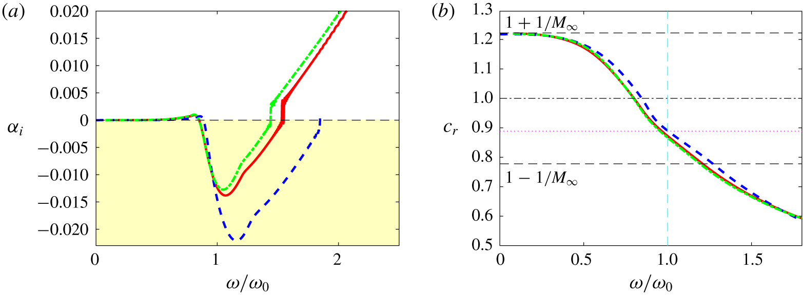
It is of interest to understand why the peak frequency of the supersonic mode is modified when using a simplified EOS. The previous analysis shows that the mode is essentially inviscid, has similar eigenfunctions and is of acoustic nature like Mack’s mode. The main difference with a subsonic second mode is that it arises from the fast mode with a weak synchronization with the slow mode. As a consequence, its phase speed decreases and attains relative supersonic values, thus generating spontaneous acoustic radiation. We recall that, for an acoustic mode, the frequency is dictated by the standing waves trapped in the waveguide between the wall and the relative sonic line. As a consequence, a thinning of the boundary layer would result in a reduction of the waveguide height and hence of the wavelength of the resonant wave.

Figure 20.

Influence of EOS model for dense gas at $M_{\infty }=4.5$ and $Re=2000$: growth rate (a) and phase speed (b) versus the non-dimensional frequency. Line legend as in table 4.

In order to estimate this wavelength for scaling purposes, we consider the compressible counterpart of the Rayleigh equation, derived from the inviscid stability equations (Mack Reference Mack1984a). Assuming 2-D disturbances and neglecting the first-order derivative term (i.e. assuming large values of the streamwise wavenumber $\unicode[STIX]{x1D6FC}$, which is strictly not fully justified but successfully used by Mack (Reference Mack1984a) and Morkovin (Reference Morkovin1987)), the equation reduces to

(4.1)$$\begin{eqnarray}\frac{\text{d}^{2}\tilde{p}}{\text{d}y^{2}}-\unicode[STIX]{x1D6FC}^{2}(1-\widetilde{M}^{2})\tilde{p}=0,\end{eqnarray}$$

where $\widetilde{M}(y)=(u(y)-c_{\unicode[STIX]{x1D711}})/a(y)$ is the relative Mach number varying in the wall-normal direction. Note that (4.1), originally derived using the perfect-gas assumption, has been shown to hold even in the case of an arbitrary equation of state (Ren et al. Reference Ren, Marxen and Pecnik2019b). The nature of the equation changes from elliptic to hyperbolic as $\widetilde{M}^{2}$ becomes greater than unity. At the sonic line ($y=y_{a}$), $\widetilde{M}(y_{a})=-1$ and, in the frame moving at the instability speed, the flow is supersonic in the upstream direction inside this layer. An approximate solution of (4.1), based on the WKB method (Mack Reference Mack1984a; Gushchin & Fedorov Reference Gushchin and Fedorov1990), imposing the nullity of the pressure gradient at the wall and the decrease of the pressure mode at infinity, yields the dispersion relation (Mack Reference Mack1984a)

(4.2)$$\begin{eqnarray}\cos \left[\unicode[STIX]{x1D6FC}_{n}\int _{0}^{y_{a}}(\widetilde{M}^{2}-1)^{1/2}\,\text{d}y\right]=0,\end{eqnarray}$$

which shows that there is an infinite sequence of discrete wavenumbers that satisfy

(4.3)$$\begin{eqnarray}\unicode[STIX]{x1D6FC}_{n}\int _{0}^{y_{a}}(\widetilde{M}^{2}-1)^{1/2}\,\text{d}y=\unicode[STIX]{x03C0}\left(n-\frac{1}{2}\right),\quad n=1,2,3,\ldots .\end{eqnarray}$$

The results are then scaled in terms of the frequency of the first standing acoustic mode ($n=1$),

(4.4)$$\begin{eqnarray}\unicode[STIX]{x1D714}_{a}=\frac{c_{r}}{2}\left(\int _{0}^{y_{a}}(\widetilde{M}^{2}-1)^{1/2}\,\text{d}y\right)^{-1},\end{eqnarray}$$

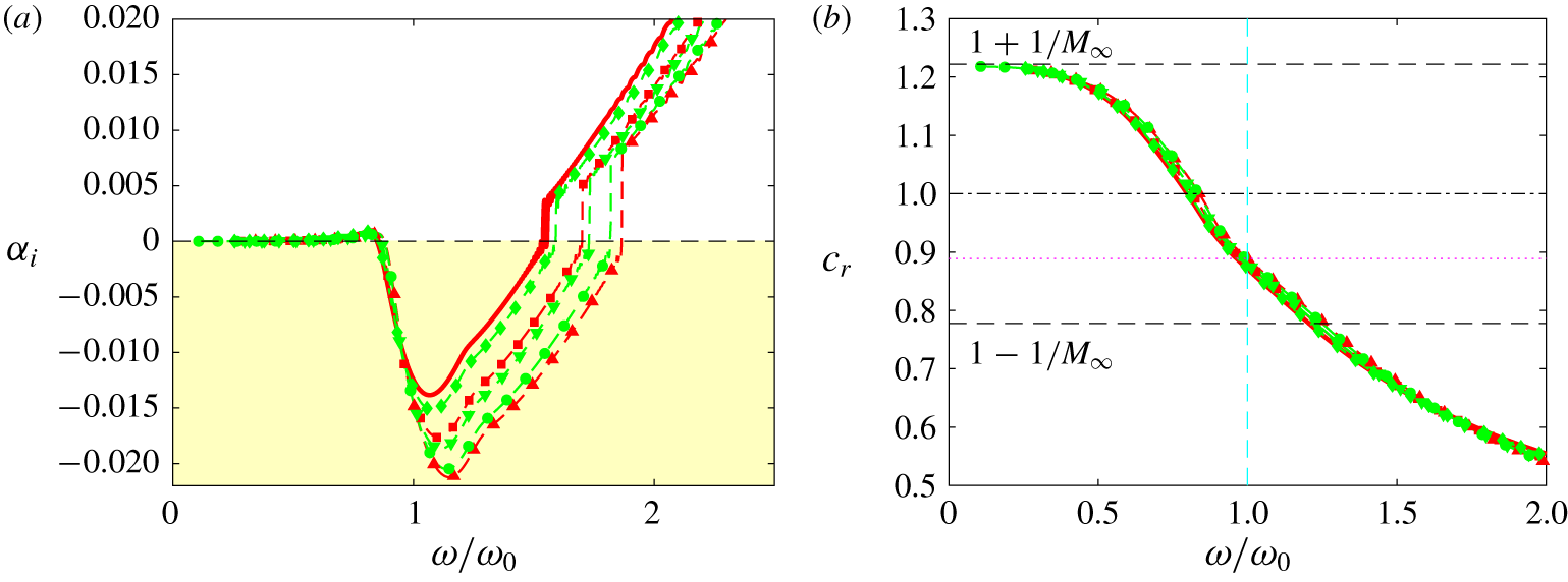
and are reported in figure 20 using the phase speed $c_{r}$ corresponding to the maximum amplification rate. A very good collapse of the phase speed is obtained, with values corresponding to the median between 1 and $1-1/M_{\infty }$ for $\unicode[STIX]{x1D714}/\unicode[STIX]{x1D714}_{a}=1$ (magenta dotted line). The growth rate has a negative peak at the acoustic frequency with a good collapse at the onset. We have also tested other scalings (not reported for the sake of brevity). In particular, we have considered scalings based on the free-stream velocity and either $\unicode[STIX]{x1D6FF}$ (the 99 % boundary-layer thickness), as suggested by Bitter & Shepherd (Reference Bitter and Shepherd2015), or $y_{a}$ (the sonic line height). The thickness of the boundary layer being weakly dependent on the gas model, the results do not collapse when using $\unicode[STIX]{x1D6FF}$ as length scale. When using $y_{a}$ the peak frequencies are fairly normalized around unity but the phase speeds do not collapse. In conclusion, a satisfactory scaling is found to be proportional to the height of the layer near the wall that acts as a waveguide where acoustic waves may become trapped.

5.1 Effect of operating conditions for PP11

A parametric study of the effect of the thermodynamic operating conditions for PP11 has been conducted. The results are presented for six points, represented in a Clapeyron’s diagram in figure 21 and whose conditions are summarized in table 5. In addition to the nominal conditions (marked by the red circle), we have considered two other operating points (in red) with the same specific volume and higher reduced pressures, so that the last point (red triangle) is outside the dense-gas region. Three additional points (in green) are characterized by the same entropy as the nominal one, but higher specific volumes. The first one (green diamond) is still inside the inversion zone and the last point (green circle) corresponds to a significantly dilute gas.

Figure 21.

Clapeyron’s diagram showing the different operating points. Symbols as in table 5. The thick black line represents the saturation curve and the thick dotted blue lines denote two isocontours of the fundamental derivative of gas dynamics $\unicode[STIX]{x1D6E4}$ (value 0 marks the boundary of the inversion zone and value 1 the boundary of the dense-gas region). The thin black lines are isentropic curves.

The base flow profiles are shown in figure 22. The streamwise velocity distributions are almost not affected by changing the operating conditions and remain close to the incompressible regime. In particular, in all cases, the boundary-layer thickness is approximately the same. The temperature increase at the wall varies from 1.4 % for the nominal case to 6.8 % for the case outside the dense-gas region. This is proportional to the value of the Eckert number for the different cases. The behaviour of the dynamic viscosity is seen to follow a liquid-like evolution in figure 22(c), with a reduced amplitude when we move away from the inversion zone. Finally, figure 22(d) presents the distributions of the generalized derivative, which are almost superimposed for all cases. A close-up view (shown in the inset) indicates, however, that a zero crossing occurs very close to the wall for the two extreme conditions (higher pressure or higher volume). The presence of these generalized inflection points would hardly affect the stability results.

Table 5.

Influence of operating point for dense gas PP11 at $M_{\infty }=4.5$: thermodynamic conditions and boundary-layer properties from similarity solutions.

Figure 22.

Similarity solutions for PP11 (dense gas) at $M_{\infty }=4.5$ for different operating points. Line legend as in table 5.

The LST results are given in figure 23 for 2-D waves at $M_{\infty }=4.5$ and $Re=2000$. For all cases, the supersonic mode has the same qualitative characteristics. However, the frequency of maximal amplification is decreased and its amplitude is enhanced as the operating point moves away from the nominal case. The frequency change can hardly be explained by modifications of the base flow velocity profiles. Furthermore, the variations of sound speed, inversely proportional to density variations, are similar for the different cases, so that the distributions of the relative Mach number $\widetilde{M}$ are weakly impacted, and the height of the acoustic waveguide $y_{a}$ is not modified substantially. The acoustic frequency $\unicode[STIX]{x1D714}_{a}$ is used to non-dimensionalize the results in figure 24. The scaling succeeds in collapsing the phase speed evolutions and the frequencies of appearance of the instability, showing that the observed differences are due to changes in the absolute value of $a$ for the various cases.

Figure 23.

Influence of operating point for PP11 at $M_{\infty }=4.5$ and $Re=2000$: growth rate (a) and phase speed (b). Line legend as in table 5.

Figure 24.

Influence of operating point for PP11 at $M_{\infty }=4.5$ and $Re=2000$: growth rate (a) and phase speed (b) versus the non-dimensional frequency. Line legend as in table 5.

5.2 Results for other dense gases

In this last section, we assess the generality of our findings for other dense gases. The working conditions for the four new gases are given in table 6. For comparison, the conditions of the nominal case for PP11 are chosen, namely $M_{\infty }=4.5$, $v_{\infty }/v_{c}=1.8$ and $T_{\infty }/T_{c}=0.995$. The thermodynamic and transport-properties models for the various gases are given in § 2.2. The main parameters of the similarity solutions are presented in table 6. Selected profiles are displayed in figure 25. The two refrigerants, R134a and R245fa (the lightest of the selected dense gases), exhibit the highest thickening and temperature variations. An interesting feature is their viscosity distributions, characterized by a mixed gas-like (close to the wall) and liquid-like behaviour. Density variations, as indicated by wall density values in table 6, are also stronger. The similarity velocity profiles for the two siloxanes, with a smaller Eckert number, are very close to each other and to that of PP11. Accordingly, temperature variations are very small. The heaviest one (D₆), which has a molecular complexity close to that of PP11, also displays a similar non-dimensional wall temperature. The plot of the generalized derivative in figure 25(d) shows up the presence of a generalized inflection point for the refrigerants, which moves away from the wall as the gas is lighter.

Table 6.

Influence of the fluid at $M_{\infty }=4.5$ with $v_{\infty }/v_{c}=1.8$ and $T_{\infty }/T_{c}=0.995$: thermodynamic conditions and boundary-layer properties from similarity solutions.

Figure 25.

Similarity solutions for different dense gases at $M_{\infty }=4.5$. Line legend as in table 6.

Figure 26.

Influence of the fluid at $M_{\infty }=4.5$ and $Re=2000$: growth rate (a) and phase speed (b). Line legend as in table 6.

The LST results in figure 26 indicate the presence of an unstable supersonic mode in a similar frequency band (approximately $\unicode[STIX]{x1D714}\approx 0.5$ for all dense gases). The phase speeds in figure 26(b) are typical of fast modes, decreasing until the speed becomes supersonic above $\unicode[STIX]{x1D714}\approx 0.6$. Some differences for the frequency or the amplitude of maximum amplification are, however, visible. For instance, the lightest gas, R134a, has the smallest frequency and amplitude and no discontinuity is visible as the mode stabilizes, indicating that the eigenvalue reaches a positive imaginary part without crossing the acoustic branch cut. The phase velocity indeed becomes supersonic when the mode is already stable. In general, the width of the unstable frequency band is narrower for gases with smaller molecular complexity. A reasonably good scaling of the results is achieved by normalizing the frequency with the pulsation of the first acoustic standing wave in the waveguide (not reported for the sake of brevity).

Figure 27.

Influence of Mach number for dense gas R134a at $Re=2000$: growth rate (a) and phase speed (b). Line legend as in table 3 (thick lines for slow modes and thin lines for fast modes).

Finally, in figure 27, we report the growth rates and phase speeds for the lightest gas R134a at various Mach numbers (values used previously for PP11, see table 3 for line legend). The overall behaviour is similar for the two dense gases. The main difference is that the supersonic mode is still stable at $M_{\infty }=3$, whereas a small unstable frequency range was observed for PP11. At $M_{\infty }=6$, the frequency of maximum amplification is lower than at $M_{\infty }=4.5$, and the rise of the unstable fast mode is accompanied by a strong stabilization of the slow mode.