1 Introduction
Green & Naghdi (Reference Green and Naghdi1976a ) proposed a set of equations, now known as the ‘Green–Naghdi (GN) equations’, to model wave propagation in fluids of finite, variable depth. Their primary objective was to develop a two-dimensional (2-D) set of equations, like the shallow-water equations, capable of modelling the parent three-dimensional (3-D) Navier–Stokes equations, even for wavelengths comparable to the fluid depth. No long-wave approximation, like that used to derive the shallow-water equations, is imposed. Green and Naghdi maintained that their model of wave propagation could also handle the problematic nonlinear inertia terms as well as general boundary conditions.
The GN equations are not derived from an asymptotic expansion in a small parameter, such as a characteristic wave slope or height to width aspect ratio. Asymptotic expansions were previously used by Stokes (Reference Stokes1847), Skjelbreia & Hendrickson (Reference Skjelbreia and Hendrickson1960) and Peregrine (Reference Peregrine1967, Reference Peregrine and Meyer1972) to study irrotational, potential flows with a free surface. Rotational flows with a free surface may be studied using the shallow-water equations, arising at first order in an asymptotic expansion in the height to width aspect ratio. Deeper flows do not appear to be amenable to such treatment. Instead, Green & Naghdi (Reference Green and Naghdi1976b ) applied Cosserat surface theory as the basis for their equations. Introduced by the Cosserat brothers (Cosserat & Cosserat Reference Cosserat and Cosserat1909), Cosserat surface theory is the theory of ‘directed fluid sheets’. This theory was first used by Green, Naghdi & Wainwright (Reference Green, Naghdi and Wainwright1965) and later by Naghdi (Reference Naghdi and Flügge1972) to study problems in continuum mechanics. This led to the development of the GN equations from the theory of directed fluid sheets (Green, Laws & Naghdi Reference Green, Laws and Naghdi1974; Green & Naghdi Reference Green and Naghdi1976b ).
In fact, credit should be given to Serre (Reference Serre1953) for the first derivation of what are commonly referred to as the ‘Green–Naghdi equations’. The well-known dispersive term in the GN momentum equations, specifically arising from the non-hydrostatic pressure (see next section), was first introduced by Serre (Reference Serre1953). The history of these equations is discussed in Dutykh et al. (Reference Dutykh, Clamond, Milewski and Mitsotakis2013) and in Castro-Orgaz & Hager (Reference Castro-Orgaz and Hager2015). To be consistent with most treatments of the subject, we nonetheless refer to the equations as the ‘GN equations’ in the present paper.
The GN equations for a homogeneous, incompressible, inviscid fluid were derived from 3-D incompressibility and energy conservation. A single approximation was made for the velocity field: it was assumed that the vertical velocity component is a linear function of the
 $z$
coordinate (parallel to gravity) and the horizontal velocity components are independent of
 $z$
. The shallow-water equations also make this assumption, but go further by assuming the pressure is determined by hydrostatic balance.
Instead of approximately satisfying the 3-D nonlinear equations (as in an asymptotic expansion), the GN equations exactly satisfy the boundary conditions, 3-D incompressibility and an integral form of energy conservation. According to Green & Naghdi (Reference Green and Naghdi1976a
), the GN equations are a specific rotational set of equations in which the horizontal flow is rotational but without vertical shear (no
 $z$
variation). Moreover, Green & Naghdi (Reference Green and Naghdi1976a
) claimed that their equations were particularly appropriate for studying the evolution of nonlinear shallow-water waves. Later, Ertekin (Reference Ertekin1984) applied the GN equations to investigate solitary wave generation and propagation in shallow water. Miles & Salmon (Reference Miles and Salmon1985) showed that the GN equations can be derived variationally from Hamilton’s principle, thereby ensuring conservation of momentum, energy and ‘potential vorticity’, a material invariant carried by every fluid particle. Miles & Salmon (Reference Miles and Salmon1985) concluded that for uniform fluid depth, the GN equations are equivalent to a generalisation of Boussinesq’s equations (Whitham Reference Whitham1967).
Shields & Webster (Reference Shields and Webster1988) applied the Kantorovich method (Kantorovich & Krylov Reference Kantorovich and Krylov1958) to develop a hierarchy of approximations of the GN equations. The velocity field was expressed as a finite sum of coefficients, depending on the horizontal coordinates
 $(x,y)$
and time
 $t$
, multiplied by weighting functions of
 $z$
, the ‘directors’. The
 $K$
th level approximation uses
 $K\geqslant 1$
such directors (Demirbilek & Webster Reference Demirbilek and Webster1999). With increasing level, the complexity of the GN equations rapidly grows. Shields & Webster (Reference Shields and Webster1988) compared the first three levels of the GN hierarchy, for steady flows depending only on one horizontal coordinate, with various orders of approximation of the Rayleigh–Boussinesq equations (Boussinesq Reference Boussinesq1871, Reference Boussinesq1877; Rayleigh Reference Rayleigh1876). Both solitary and periodic wave solutions were compared. Shields & Webster (Reference Shields and Webster1988) found that the GN equations converge rapidly with increasing level, and that the solutions become increasingly irrotational. Zhao & Duan (Reference Zhao and Duan2010) revealed that the higher-level GN equations (up to the third level) generate more accurate predictions of fully nonlinear shallow water waves as the waves shoal and interact with a plane beach. For small amplitude shallow-water waves, Webster, Duan & Zhao (Reference Webster, Duan and Zhao2011) demonstrated that the most accurate form of the dispersion relation is found for the GN equations at the highest level (they examined up to the seventh level).
Nevertheless, the great complexity of the GN equations beyond the first level has virtually prohibited their use in studies of time-dependent nonlinear flows depending on both horizontal coordinates. This led Zhao & Duan (Reference Zhao and Duan2010), Webster et al. (Reference Webster, Duan and Zhao2011), Zhao, Duan & Ertekin (Reference Zhao, Duan and Ertekin2014) and Zhao et al. (Reference Zhao, Duan, Ertekin and Hayatdavoodi2015) to simplify the higher-level GN equations by discarding high derivative terms in order to make any headway. These simplified equations are not derivable from a variational principle, so there is no guarantee of basic conservation of energy, etc. As the focus in this work is on the original GN equations, we do not consider the higher levels or their simplifications further. In what follows, we refer to the first-level GN equations as simply the ‘GN equations’.
The GN equations are computationally challenging due to their implicit form. Le Métayer, Gavrilyuk & Hank (Reference Le Métayer, Gavrilyuk and Hank2010) proposed a hybrid numerical solver of the GN equations by applying a Godunov scheme. Bonneton et al. (Reference Bonneton, Chazel, Lannes, Marche and Tissier2011) developed a shock-capturing scheme to solve the GN equations for shallow-water waves of large amplitude. For applications to geophysical flows (where the Coriolis acceleration plays a major role), Pearce & Esler (Reference Pearce and Esler2010) derived a form of the GN equations which uses height, horizontal divergence and vertical vorticity as prognostic variables. Pearce & Esler (Reference Pearce and Esler2010) used a pseudo-spectral algorithm and an implicit iterative method to compute the prognostic variable tendencies. The present paper uses a similar approach but for a different set of prognostic variables.
The main focus here is on the regularity of the GN equations. To date, there have been few systematic studies of the convergence of the GN equations with increasing numerical resolution – and without any viscous (or implied numerical) regularisation (some results for non-rotating flows can be found in Jalali Reference Jalali2016). It is often assumed that the small scales play at most a minor role, as for instance found in many two-dimensional flow models including the shallow-water equations (see, e.g. Dritschel et al. Reference Dritschel, Scott, Macaskill, Gottwald and Tran2009; Dritschel, Gottwald & Oliver Reference Dritschel, Gottwald and Oliver2017), for which no viscous regularisation is necessary. Mathematically, it is important to establish the regularity of a given set of partial differential equations (PDEs), i.e. whether solutions to the PDEs exist for all time starting from sufficiently smooth initial data. For the GN equations, there is no mathematical proof, and it may be elusive given the degree of nonlinearity of the equations. In lieu of this, the present study aims to provide detailed numerical evidence questioning the regularity of the GN equations. Notably, rotation generally suppresses nonlinear scale cascades in the simpler shallow-water equations (which we also study; see also Dritschel et al. Reference Dritschel, Gottwald and Oliver2017). Thus, a priori, we anticipate rotation is also beneficial for the GN equations.
The paper is organised as follows. The GN equations are stated in § 2 and then transformed to a more convenient form for studying rotating shallow-water flow, a widely studied model of large-scale atmospheric and oceanic flows (Gill Reference Gill1982; Vallis Reference Vallis2008). In particular, the transformed equations make explicit use of the material conservation of potential vorticity, a fundamental Lagrangian invariant, together with a pair of variables expressing the first-order departure from geostrophic–hydrostatic balance first introduced by Mohebalhojeh & Dritschel (Reference Mohebalhojeh and Dritschel2001). These variables are a natural starting point for decomposing the fluid motion into balanced and imbalanced components, associated with slow vortical motions and relatively fast gravity waves, respectively. This decomposition has been instrumental for understanding planetary circulations and geophysical fluid dynamics in general (Norbury Reference Norbury and Roulstone2002a ,Reference Norbury and Roulstone b ), and is crucial for interpreting the results in § 3. There, we identify features of the GN flow at small scales (horizontal scales smaller than the mean fluid depth) that exhibit poor convergence (or no convergence) with increasing numerical resolution. Comparisons with solutions of the shallow-water equations, obtained using identical numerical methods, furthermore reveal the terms in the GN equations responsible for the poor convergence. Our conclusions are offered in § 4. We advocate modifying the GN equations to improve convergence while preserving their more accurate dispersion characteristics at horizontal scales comparable to the mean fluid depth.
2 The GN equations recast
Following Pearce & Esler (Reference Pearce and Esler2010), we consider the GN equations for a rotating layer of fluid lying on a flat bottom at
 $z=0$
. With
 $h(\boldsymbol{x},t)$
the height of the free surface and
 $\boldsymbol{u}(\boldsymbol{x},t)=(u(\boldsymbol{x},t),v(\boldsymbol{x},t))$
the height-independent horizontal velocity, the equations take the form
 $$\begin{eqnarray}\displaystyle & \displaystyle D\boldsymbol{u}+f\boldsymbol{k}\times \boldsymbol{u}=-g\unicode[STIX]{x1D735}h-\frac{1}{3h}\unicode[STIX]{x1D735}(h^{2}D^{2}h), & \displaystyle\end{eqnarray}$$
 $$\begin{eqnarray}\displaystyle & \displaystyle Dh+h\unicode[STIX]{x1D735}\boldsymbol{\cdot }\boldsymbol{u}=0, & \displaystyle\end{eqnarray}$$
where
 $\boldsymbol{x}=(x,y)$
is the horizontal position vector,
 $t$
is time,
 $\boldsymbol{k}$
is the vertical unit vector,
 $D=\unicode[STIX]{x2202}/\unicode[STIX]{x2202}t+\boldsymbol{u}\boldsymbol{\cdot }\unicode[STIX]{x1D735}$
is the material derivative,
 $g$
is the gravitational acceleration and
 $f$
is the constant Coriolis frequency (see e.g. Pearce & Esler Reference Pearce and Esler2010).
The nonlinear term on the right-hand side of (2.1) makes the equations fundamentally implicit and challenging to solve. This term represents non-hydrostatic pressure effects, and is absent in the corresponding shallow-water (SW) equations (this is the only difference between the GN and SW equations). While
 $Dh=-h\unicode[STIX]{x1D735}\boldsymbol{\cdot }\boldsymbol{u}$
from (2.2), a second application of the material derivative
 $D$
generates time derivatives of
 $\boldsymbol{u}$
. It is not possible to explicitly solve for these time derivatives in (2.1). Nonetheless, many numerical methods have been developed to cope with this difficulty.
In this paper, we wish to explore the differences between the solutions to the GN and the SW equations in order to better understand the role played by the above non-hydrostatic pressure term in the nonlinear dynamics. It is well known that the linearised GN equations (about a state of rest) better approximate the dispersion relation for a finite depth fluid than do the linearised SW equations (Webster et al. Reference Webster, Duan and Zhao2011). Here the focus is on the nonlinear behaviour of the solutions.
To this end, it is helpful to recast the GN equations into a form which permits more accurate numerical solutions of rotating shallow-water flows when the Rossby number
 $Ro\ll 1$
(Mohebalhojeh & Dritschel Reference Mohebalhojeh and Dritschel2000, Reference Mohebalhojeh and Dritschel2001). The Rossby number is the ratio of a characteristic vertical vorticity
 $\unicode[STIX]{x1D701}=v_{x}-u_{y}$
to the Coriolis frequency
 $f$
(subscripts
 $x$
and
 $y$
denote differentiation). The small Rossby number regime is an extensively well-studied regime of geophysical fluid dynamics, due to its relevance to atmospheric and oceanic dynamics, and potentially to other planetary atmospheres (see Gill (Reference Gill1982), Ford, McIntyre & Norton (Reference Ford, McIntyre and Norton2000), Norbury (Reference Norbury and Roulstone2002b
), Vallis (Reference Vallis2008) and Read (Reference Read2011) for a sample of the vast literature).
Past studies of rotating shallow-water flows in both planar and spherical geometry have identified a particular set of variables having both significant theoretical and computational advantages over the traditional set
 $(h,u,v)$
. These new variables consist of the Rossby–Ertel potential vorticity
 $q$
and a pair of other variables expressing the departure from geostrophic–hydrostatic balance at first order, namely the divergence
 $\unicode[STIX]{x1D6FF}=\unicode[STIX]{x1D735}\boldsymbol{\cdot }\boldsymbol{u}=u_{x}+v_{y}$
and the acceleration divergence
 $\unicode[STIX]{x1D6FE}=\unicode[STIX]{x1D735}\boldsymbol{\cdot }(D\boldsymbol{u})$
(Mohebalhojeh & Dritschel Reference Mohebalhojeh and Dritschel2001; Smith & Dritschel Reference Smith and Dritschel2006; Mohebalhojeh & Dritschel Reference Mohebalhojeh and Dritschel2007; Dritschel et al.
Reference Dritschel, Gottwald and Oliver2017). Their theoretical advantage is that they allow one to separate, to leading order, fundamentally distinct dynamical motions: ‘slow’ vortical motions induced by potential vorticity and ‘fast’ inertia–gravity wave motions arising from departures from geostrophic–hydrostatic balance (or geostrophic balance in the SW equations which assume hydrostatic balance). In fact, the
 $(q,\unicode[STIX]{x1D6FF},\unicode[STIX]{x1D6FE})$
variable set forms a convenient basis for separating flows into ‘balanced’ and ‘imbalanced’ components, the former controlled by potential vorticity and the latter consisting of the residual motions identified as inertia–gravity waves (IGWs). The balanced component is determined by a pair of balance conditions such as
 $\unicode[STIX]{x1D6FF}_{t}=\unicode[STIX]{x1D6FE}_{t}=0$
(the subscript
 $t$
denotes partial differentiation with respect to time), and the imbalanced component is the residual flow. The balance conditions effectively filter out the IGWs. While the estimate of balance depends on the balance conditions chosen (albeit weakly for
 $Ro\ll 1$
), this separation is nevertheless fruitful for understanding IGW emission and the breakdown of balance (see e.g. Dritschel & Vanneste Reference Dritschel and Vanneste2006).
Computationally, the
 $(q,\unicode[STIX]{x1D6FF},\unicode[STIX]{x1D6FE})$
variable set also offers significant advantages over the traditional set
 $(h,u,v)$
as well as the commonly used vorticity-divergence set
 $(h,\unicode[STIX]{x1D701},\unicode[STIX]{x1D6FF})$
in the SW equations (Mohebalhojeh & Dritschel Reference Mohebalhojeh and Dritschel2001; Smith & Dritschel Reference Smith and Dritschel2006; Mohebalhojeh & Dritschel Reference Mohebalhojeh and Dritschel2007; Dritschel et al.
Reference Dritschel, Gottwald and Oliver2017). First of all, material conservation of potential vorticity can be made explicit, using highly accurate Lagrangian contour-advection methods (Dritschel & Ambaum Reference Dritschel and Ambaum1997; Dritschel & Fontane Reference Dritschel and Fontane2010). Secondly, the height field
 $h$
is diagnosed rather than prognosed. It is diagnosed from the definition of potential vorticity. This avoids the generation of erroneous IGWs from discretisation errors in (2.2). These errors obscure the natural, but often exceedingly weak, spontaneous emission of IGWs from the balanced vortical motions. The result is a more accurate representation of both the balanced and the imbalanced dynamics, at minimal extra computational cost.
2.1 The GN equations in
 $(q,\unicode[STIX]{x1D6FF},\unicode[STIX]{x1D6FE})$
variables

We next develop the prognostic (or time-evolution) equations for potential vorticity
 $q$
, divergence
 $\unicode[STIX]{x1D6FF}=\unicode[STIX]{x1D735}\boldsymbol{\cdot }\boldsymbol{u}$
and acceleration divergence
 $\unicode[STIX]{x1D6FE}=\unicode[STIX]{x1D735}\boldsymbol{\cdot }(D\boldsymbol{u})$
. Potential vorticity (PV) satisfies material conservation
 $$\begin{eqnarray}\displaystyle Dq=0, & & \displaystyle\end{eqnarray}$$
which is a consequence of the particle-relabelling symmetry of the GN equations (and many other equations used in studies of geophysical fluid dynamics). The PV is defined by
 $$\begin{eqnarray}\displaystyle q & = & \displaystyle \frac{\unicode[STIX]{x1D701}+f}{h}+\frac{1}{3}\boldsymbol{k}\boldsymbol{\cdot }(\unicode[STIX]{x1D735}(Dh)\times \unicode[STIX]{x1D735}h)\nonumber\\ \displaystyle & = & \displaystyle \frac{\unicode[STIX]{x1D701}+f}{h}+\frac{1}{3}J(h,\unicode[STIX]{x1D6FF}),\end{eqnarray}$$
where
 $J(a,b)=a_{x}b_{y}-a_{y}b_{x}$
for any two scalar fields
 $a$
and
 $b$
(Pearce & Esler Reference Pearce and Esler2010). Here
 $Dh=-h\unicode[STIX]{x1D6FF}$
has been used from (2.2). The Jacobian term here is absent in the corresponding SW PV.
The divergence equation is found from the definition of acceleration divergence
 $\unicode[STIX]{x1D6FE}$
,
 $$\begin{eqnarray}\displaystyle \unicode[STIX]{x1D6FE}=\unicode[STIX]{x1D735}\boldsymbol{\cdot }(D\boldsymbol{u})=\unicode[STIX]{x1D6FF}_{t}+\unicode[STIX]{x1D735}\boldsymbol{\cdot }(\unicode[STIX]{x1D6FF}\boldsymbol{u})-2J(u,v), & & \displaystyle\end{eqnarray}$$
which can be rearranged to give
 $$\begin{eqnarray}\displaystyle \unicode[STIX]{x1D6FF}_{t}=\unicode[STIX]{x1D6FE}-\unicode[STIX]{x1D735}\boldsymbol{\cdot }(\unicode[STIX]{x1D6FF}\boldsymbol{u})+2J(u,v). & & \displaystyle\end{eqnarray}$$
This equation is identical to that appearing in the SW model.
The explicit form of
 $\unicode[STIX]{x1D6FE}$
is obtained by taking the divergence of (2.1) yielding
 $$\begin{eqnarray}\displaystyle \unicode[STIX]{x1D6FE}=f\unicode[STIX]{x1D701}-g\unicode[STIX]{x1D6FB}^{2}h+{\textstyle \frac{1}{3}}\unicode[STIX]{x1D6FB}^{2}(hD(h\unicode[STIX]{x1D6FF}))+{\textstyle \frac{1}{3}}\unicode[STIX]{x1D735}\boldsymbol{\cdot }(\unicode[STIX]{x1D735}h\,D(h\unicode[STIX]{x1D6FF})), & & \displaystyle\end{eqnarray}$$
where
 $\unicode[STIX]{x1D6FB}^{2}$
is Laplace’s operator and the relative vorticity
 $\unicode[STIX]{x1D701}$
is
 $$\begin{eqnarray}\displaystyle \unicode[STIX]{x1D701}=h\left(q-{\textstyle \frac{1}{3}}J(h,\unicode[STIX]{x1D6FF})\right)-f & & \displaystyle\end{eqnarray}$$
from the definition of PV in (2.4). All of the terms multiplied by
 $1/3$
in the above equations are absent in the corresponding SW equations. These extra terms make (2.7) implicit. Using
 $$\begin{eqnarray}\displaystyle D(h\unicode[STIX]{x1D6FF})=h\tilde{\unicode[STIX]{x1D6FE}}\quad \text{where}~\tilde{\unicode[STIX]{x1D6FE}}\equiv \unicode[STIX]{x1D6FE}+2J(u,v)-2\unicode[STIX]{x1D6FF}^{2}, & & \displaystyle\end{eqnarray}$$
which comes from combining
 $Dh=-h\unicode[STIX]{x1D6FF}$
, i.e. (2.2), with (2.6), we can eliminate all time derivatives in the definition of
 $\unicode[STIX]{x1D6FE}$
:
 $$\begin{eqnarray}\displaystyle \unicode[STIX]{x1D6FE}=f\unicode[STIX]{x1D701}-g\unicode[STIX]{x1D6FB}^{2}h+{\textstyle \frac{1}{3}}\unicode[STIX]{x1D6FB}^{2}(h^{2}\tilde{\unicode[STIX]{x1D6FE}})+{\textstyle \frac{1}{3}}\unicode[STIX]{x1D735}\boldsymbol{\cdot }(h\tilde{\unicode[STIX]{x1D6FE}}\unicode[STIX]{x1D735}h). & & \displaystyle\end{eqnarray}$$
While we cannot solve for
 $\unicode[STIX]{x1D6FE}$
explicitly, in fact this equation is only used to determine
 $h$
as part of the inversion procedure discussed in § 2.2.
The evolution equation for
 $\unicode[STIX]{x1D6FE}$
is found by taking a partial time derivative of (2.10). This gives
 $$\begin{eqnarray}\displaystyle \unicode[STIX]{x1D6FE}_{t}=f\unicode[STIX]{x1D701}_{t}-g\unicode[STIX]{x1D6FB}^{2}h_{t}+{\textstyle \frac{1}{3}}\unicode[STIX]{x1D6FB}^{2}(2hh_{t}\tilde{\unicode[STIX]{x1D6FE}}+h^{2}\tilde{\unicode[STIX]{x1D6FE}}_{t})+{\textstyle \frac{1}{3}}\unicode[STIX]{x1D735}\boldsymbol{\cdot }(\tilde{\unicode[STIX]{x1D6FE}}\unicode[STIX]{x1D735}(hh_{t})+h\tilde{\unicode[STIX]{x1D6FE}}_{t}\unicode[STIX]{x1D735}h), & & \displaystyle\end{eqnarray}$$
where the time derivatives in (2.11) are
 $$\begin{eqnarray}\displaystyle & \displaystyle \unicode[STIX]{x1D701}_{t}=-\unicode[STIX]{x1D735}\boldsymbol{\cdot }((\unicode[STIX]{x1D701}+f)\boldsymbol{u})+\frac{h}{3}J(h,\tilde{\unicode[STIX]{x1D6FE}}), & \displaystyle\end{eqnarray}$$
 $$\begin{eqnarray}\displaystyle & \displaystyle h_{t}=-\unicode[STIX]{x1D735}\boldsymbol{\cdot }(h\boldsymbol{u}), & \displaystyle\end{eqnarray}$$
 $$\begin{eqnarray}\displaystyle & \displaystyle \tilde{\unicode[STIX]{x1D6FE}}_{t}=\unicode[STIX]{x1D6FE}_{t}+2J(u_{t},v)+2J(u,v_{t})-4\unicode[STIX]{x1D6FF}\unicode[STIX]{x1D6FF}_{t}, & \displaystyle\end{eqnarray}$$
 $$\begin{eqnarray}\displaystyle & \displaystyle u_{t}=-\boldsymbol{u}\boldsymbol{\cdot }\unicode[STIX]{x1D735}u+fv-gh_{x}+\frac{1}{3h}(h^{3}\tilde{\unicode[STIX]{x1D6FE}})_{x}, & \displaystyle\end{eqnarray}$$
 $$\begin{eqnarray}\displaystyle & \displaystyle v_{t}=-\boldsymbol{u}\boldsymbol{\cdot }\unicode[STIX]{x1D735}v-fu-gh_{y}+\frac{1}{3h}(h^{3}\tilde{\unicode[STIX]{x1D6FE}})_{y}, & \displaystyle\end{eqnarray}$$
while
 $\unicode[STIX]{x1D6FF}_{t}$
is given in (2.6). It is not possible to obtain
 $\unicode[STIX]{x1D6FE}_{t}$
directly and so iteration is generally required (see appendix B). The corresponding SW equations in
 $(q,\unicode[STIX]{x1D6FF},\unicode[STIX]{x1D6FE})$
variables are found by dropping all terms multiplied by the factor
 $1/3$
. Then,
 $\unicode[STIX]{x1D6FE}_{t}$
is explicit.
2.2 Inversion
As the height field
 $h$
and velocity field
 $\boldsymbol{u}$
are not explicitly evolved, they must be obtained from the definitions of
 $q$
,
 $\unicode[STIX]{x1D6FF}$
and
 $\unicode[STIX]{x1D6FE}$
by a process called ‘inversion’. The velocity field is decomposed into a domain-mean part
 $\boldsymbol{U}(t)$
, a non-divergent part expressed in terms of a streamfunction
 $\unicode[STIX]{x1D713}$
and a divergent part expressed in terms of a potential
 $\unicode[STIX]{x1D712}$
:
 $$\begin{eqnarray}\displaystyle u=U-\unicode[STIX]{x1D713}_{y}+\unicode[STIX]{x1D712}_{x};\quad v=V+\unicode[STIX]{x1D713}_{x}+\unicode[STIX]{x1D712}_{y}. & & \displaystyle\end{eqnarray}$$
Then
 $\unicode[STIX]{x1D713}$
and
 $\unicode[STIX]{x1D712}$
are found from
 $$\begin{eqnarray}\displaystyle \unicode[STIX]{x1D6FB}^{2}\unicode[STIX]{x1D713}=\unicode[STIX]{x1D701};\quad \unicode[STIX]{x1D6FB}^{2}\unicode[STIX]{x1D712}=\unicode[STIX]{x1D6FF}, & & \displaystyle\end{eqnarray}$$
where
 $\unicode[STIX]{x1D701}$
is defined in (2.8). In the doubly periodic domain considered, these equations are readily solved algebraically after a Fourier transform (see appendix A).
The mean flow
 $\boldsymbol{U}(t)$
is determined by the condition of zero (relative) momenta,
 $\langle h\boldsymbol{u}\rangle =0$
(here
 $\langle \cdot \rangle$
denotes a domain average). As shown in § 2.3, if these momenta are zero initially, they remain zero. Defining
 $H=\langle h\rangle$
to be the mean fluid height (a constant) and decomposing
 $h$
as
 $H(1+\tilde{h})$
where
 $\tilde{h}$
is a dimensionless anomaly, the condition
 $\langle h\boldsymbol{u}\rangle =0$
implies
 $$\begin{eqnarray}\displaystyle \langle (1+\tilde{h})\boldsymbol{u}\rangle =0\quad \Rightarrow \quad \boldsymbol{U}=-\langle \tilde{h}\tilde{\boldsymbol{u}}\rangle , & & \displaystyle\end{eqnarray}$$
where
 $\tilde{\boldsymbol{u}}$
is the part of
 $\boldsymbol{u}$
with zero mean, i.e. the part involving
 $\unicode[STIX]{x1D713}$
and
 $\unicode[STIX]{x1D712}$
in (2.17). Hence,
 $\boldsymbol{U}$
is fully determined from
 $\tilde{h}$
,
 $\unicode[STIX]{x1D713}$
and
 $\unicode[STIX]{x1D712}$
.
The potential
 $\unicode[STIX]{x1D712}$
, and hence the divergent part of the velocity field
 $\unicode[STIX]{x1D735}\unicode[STIX]{x1D712}$
, are found directly from
 $\unicode[STIX]{x1D6FF}$
. However,
 $\unicode[STIX]{x1D713}$
and the remaining part of the velocity field cannot be found without knowledge of
 $h$
since
 $\unicode[STIX]{x1D701}$
depends on
 $h$
(as well as on
 $q$
and
 $\unicode[STIX]{x1D6FF}$
) in (2.8). To determine
 $h$
, we use the definition of
 $\unicode[STIX]{x1D6FE}$
in (2.10). Rearranging this equation and replacing
 $\unicode[STIX]{x1D701}$
by its explicit dependence on
 $h$
,
 $q$
and
 $\unicode[STIX]{x1D6FF}$
, we obtain
 $$\begin{eqnarray}\displaystyle g\unicode[STIX]{x1D6FB}^{2}h-fqh+f^{2}=-\unicode[STIX]{x1D6FE}-{\textstyle \frac{1}{3}}fhJ(h,\unicode[STIX]{x1D6FF})+{\textstyle \frac{1}{3}}\unicode[STIX]{x1D6FB}^{2}(h^{2}\tilde{\unicode[STIX]{x1D6FE}})+{\textstyle \frac{1}{3}}\unicode[STIX]{x1D735}\boldsymbol{\cdot }(h\tilde{\unicode[STIX]{x1D6FE}}\unicode[STIX]{x1D735}h). & & \displaystyle\end{eqnarray}$$
This is an implicit, nonlinear equation for
 $h$
(the solution method used for it is described in appendix A). The corresponding SW form of this equation only has
 $-\unicode[STIX]{x1D6FE}$
on the right-hand side. The SW equation is elliptic if the PV
 $q\geqslant 0$
everywhere, which is guaranteed by material conservation of PV when
 $q\geqslant 0$
initially. The ellipticity of the GN equation is uncertain, but according to the numerical results presented in the next section, it appears to be satisfied when the nonlinear GN terms on the right-hand side are not dominant.
The SW form of (2.20) is linear in
 $h$
and thus a unique solution may be readily found. But the GN form is nonlinear in
 $h$
and moreover couples to
 $u$
and
 $v$
. The result is a coupled set of nonlinear elliptic equations for
 $h$
,
 $u$
and
 $v$
which must be solved iteratively (details may be found in appendix A).
2.3 Conservation
The inviscid, unforced GN equations like their SW counterparts conserve mass, energy and an infinite set of Casimirs associated with material conservation of PV. Depending on the boundary conditions, they also conserve momentum (in
 $x$
and
 $y$
) and angular momentum.
Conservation of mass means that
 $\langle h\rangle$
, the mean height of the fluid
 $H$
, remains constant since the GN and SW equations both assume that the fluid has uniform density. This is simply shown by taking an average of (2.2).
Conservation of energy implies
 $$\begin{eqnarray}\displaystyle {\mathcal{H}}=\frac{A}{2}\left\langle h\left(\Vert \boldsymbol{u}\Vert ^{2}+gh+{\textstyle \frac{1}{3}}h^{2}\unicode[STIX]{x1D6FF}^{2}\right)\right\rangle & & \displaystyle\end{eqnarray}$$
remains constant (
 $A$
is the domain area). This is actually the Hamiltonian from which one may derive the equations of motion (Miles & Salmon Reference Miles and Salmon1985). Its conservation may be demonstrated by taking the inner product of (2.1) with
 $h\boldsymbol{u}$
and averaging over the domain. In the SW equations, the term involving
 $\unicode[STIX]{x1D6FF}^{2}$
is absent. Conservation of energy arises from time-translational invariance of the equations.
Material conservation of PV (cf. (2.3)) implies that any mass-weighted functional of PV is conserved:
 $$\begin{eqnarray}\displaystyle {\mathcal{C}}=\langle hF(q)\rangle , & & \displaystyle\end{eqnarray}$$
where
 $F$
is an arbitrary convex function. This follows by averaging (2.3) multiplied by
 $h$
and using (2.2). Conservation of these Casimirs arises from particle-relabelling symmetry.
In an infinite domain, both momentum and angular momentum are conserved. Since the background flow is rotating uniformly at rate
 $\unicode[STIX]{x1D6FA}=f/2$
, conservation of momentum implies
 $$\begin{eqnarray}\displaystyle {\mathcal{M}}^{x}=\langle h(u-fy)\rangle \quad \text{and}\quad {\mathcal{M}}^{y}=\langle h(v+fx)\rangle & & \displaystyle\end{eqnarray}$$
are both conserved. This follows by averaging
 $h$
times (2.1) and using (2.2). Conservation of momentum arises from space-translational invariance of the equations.
In a doubly periodic domain such as considered in the present work,
 ${\mathcal{M}}^{x}$
and
 ${\mathcal{M}}^{y}$
are not conserved. However, the relative momenta
 $\langle hu\rangle$
and
 $\langle hv\rangle$
obey
 $$\begin{eqnarray}\displaystyle \frac{\text{d}\langle hu\rangle }{\text{d}t}=f\langle hv\rangle \quad \text{and}\quad \frac{\text{d}\langle hv\rangle }{\text{d}t}=-f\langle hu\rangle & & \displaystyle\end{eqnarray}$$
i.e. they exhibit an inertial oscillation at frequency
 $f$
. This means that their squared magnitude
 $\langle hu\rangle ^{2}+\langle hv\rangle ^{2}$
is conserved. It is natural to set this to zero, for then the mean flow
 $\boldsymbol{U}=\langle \boldsymbol{u}\rangle$
is determined from
 $\langle hu\rangle =\langle hv\rangle =0$
, see (2.19).
Finally, the conserved angular momentum in an infinite domain, or in any circularly symmetric domain is given by
 $$\begin{eqnarray}\displaystyle {\mathcal{J}}=\langle h\boldsymbol{k}\boldsymbol{\cdot }(\boldsymbol{x}\times (\boldsymbol{u}+\unicode[STIX]{x1D6FA}\boldsymbol{k}\times \boldsymbol{x}))\rangle =\langle h(xv-yu+\unicode[STIX]{x1D6FA}(x^{2}+y^{2}))\rangle . & & \displaystyle\end{eqnarray}$$
Again, conservation of
 ${\mathcal{J}}$
can be shown by manipulating equations (2.2) and (2.1), integrating by parts repeatedly. Conservation of angular momentum arises from rotational invariance of the equations. In a doubly periodic domain,
 ${\mathcal{J}}$
is not conserved.
Except for energy, all of the conserved quantities have the same form in the GN and SW equations.
3 Results
We study the evolution of an unstable jet or zonal current in a doubly periodic domain
 $-\unicode[STIX]{x03C0}\leqslant x,y<\unicode[STIX]{x03C0}$
. This a classical paradigm used in geophysical fluid dynamics to study shear instabilities, vortex roll-up, merger and mixing, processes central to the dynamics of the atmosphere, the oceans and other planetary atmospheres (see Juckes & McIntyre Reference Juckes and McIntyre1987; Waugh & Dritschel Reference Waugh and Dritschel1991; Thomson Reference Thomson2008; Thomson & McIntyre Reference Thomson and McIntyre2016, and references therein). Rotation and stratification both play leading-order roles in shaping planetary circulations across a wide range of spatial scales (Gill Reference Gill1982; Vallis Reference Vallis2008; Read Reference Read2011). These effects tend to regularise the dynamics by suppressing relatively high-frequency motions associated with inertia–gravity and acoustic waves, leaving predominantly low frequency motions dominated by the advection of PV (Hoskins, McIntyre & Robertson Reference Hoskins, McIntyre and Robertson1985; Ford et al.
Reference Ford, McIntyre and Norton2000). This state of affairs is called ‘balance’, a hypothetical state entirely determined by the distribution of PV, a single scalar field. For example, neglecting the horizontal and vertical acceleration in the momentum equations gives rise to geostrophic and hydrostatic balance, respectively. However, this balance is only the leading-order approximation to the actual balance exhibited by typical nonlinear flows (see Mohebalhojeh & Dritschel Reference Mohebalhojeh and Dritschel2001; Viúdez & Dritschel Reference Viúdez and Dritschel2004; Dritschel & McKiver Reference Dritschel and McKiver2015, and references therein). In the results below, we investigate for the first time the nature of balance in the GN equations, starting either from an initially imbalanced state or a balanced one.
We compare GN and SW simulations carried out at two different resolutions,
 $256\times 256$
and
 $512\times 512$
. The effective resolution is approximately 16 times higher due to the use of the combined Lagrangian advection method (Dritschel & Fontane Reference Dritschel and Fontane2010), as explained in appendix C and demonstrated by Dritschel & Tobias (Reference Dritschel and Tobias2012) for 2-D magnetohydrodynamic turbulence in a direct comparison with the standard pseudo-spectral method. Similar gains in resolution were found by Dritschel, Qi & Marston (Reference Dritschel, Qi and Marston2015) for two-dimensional turbulence on a sphere.
All simulations use the same physical and numerical parameters for a given resolution. We take the Coriolis frequency to be
 $f=4\unicode[STIX]{x03C0}$
so that one unit of time corresponds to the rotation period of the background uniformly rotating flow. Gravity
 $g$
only appears in the combination
 $c^{2}=gH$
when the equations are written using the dimensionless height anomaly
 $\tilde{h}=(h-H)/H$
and the PV anomaly
 $\tilde{q}=Hq-f$
(see appendix A). In the SW equations,
 $c$
corresponds to the short-scale gravity-wave speed. This is taken to be
 $c=2\unicode[STIX]{x03C0}$
. The ratio
 $c/f$
, known as the Rossby deformation length
 $L_{D}$
, is then 0.5. Scales larger than this are strongly affected by rotation (see e.g. Vallis Reference Vallis2008). The SW equations depend on no other physical parameters. However, the GN equations depend explicitly on the mean depth, independently of
 $c^{2}$
(see appendix A). Here we take
 $H=0.2$
, comparable to but smaller than
 $L_{D}$
. The effect of variations in these parameters is discussed below in § 3.5. The numerical parameters used are given in appendix D.
The initial flow state is prescribed through the PV anomaly
 $\tilde{q}$
together with either
 $\unicode[STIX]{x1D6FF}=\unicode[STIX]{x1D6FE}=0$
, or non-zero
 $\unicode[STIX]{x1D6FF}$
and
 $\unicode[STIX]{x1D6FE}$
determined from the balance conditions
 $\unicode[STIX]{x1D6FF}_{t}=\unicode[STIX]{x1D6FE}_{t}=0$
, as elaborated in § 3.2. By the inversion procedure detailed in appendix A, we can then obtain
 $\tilde{h}$
,
 $u$
and
 $v$
initially. The specific initial PV anomaly field considered has a parabolic profile in
 $y$
,
 $$\begin{eqnarray}\displaystyle \tilde{q}(\boldsymbol{x},0)=\frac{4(y_{2}(x)-y)(y-y_{1}(x))}{(y_{2}(x)-y_{1}(x))^{2}}f+Q & & \displaystyle\end{eqnarray}$$
for
 $y_{1}(x)<y<y_{2}(x)$
and
 $\tilde{q}=Q$
otherwise. Here
 $Q$
is a constant chosen to satisfy the mathematical requirement that the domain-integrated relative vorticity
 $\unicode[STIX]{x1D701}=v_{x}-u_{y}$
be zero (this constant is determined as part of the inversion procedure, see appendix A). The functions
 $y_{1}(x)$
and
 $y_{2}(x)$
are chosen to impart a weak, non-zonal perturbation on the initial flow, allowing instabilities to grow. We take
 $$\begin{eqnarray}\displaystyle y_{1}=-{\textstyle \frac{1}{2}}w\quad \text{and}\quad y_{2}={\textstyle \frac{1}{2}}w+a_{2}\sin 2x+a_{3}\sin 3x, & & \displaystyle\end{eqnarray}$$
with parameters
 $w=0.4$
(the average jet width),
 $a_{2}=0.02$
and
 $a_{3}=-0.01$
. Note: the maximum value of
 $\tilde{q}$
exceeds the background value by
 $f=4\unicode[STIX]{x03C0}$
.
The flow regime considered is strongly ageostrophic, as measured by the initial Rossby and Froude numbers,
 $Ro=|\unicode[STIX]{x1D701}|_{max}/f$
and
 $Fr=(\Vert \boldsymbol{u}\Vert /\sqrt{gh})_{max}$
. For the GN simulations starting with
 $\unicode[STIX]{x1D6FF}=\unicode[STIX]{x1D6FE}=0$
or with
 $\unicode[STIX]{x1D6FF}_{t}=\unicode[STIX]{x1D6FE}_{t}=0$
, we find
 $Ro\approx 0.66$
and
 $Fr\approx 0.18$
. These values rise to approximately 0.75 and 0.23 over the course of the evolution. Closely similar values are found in the SW simulations.
3.1 Flow evolution and model inter-comparison
We begin by a qualitative description of the flow evolution. We illustrate the PV field at several characteristic times in figure 1. This is for the GN dynamics starting from
 $\unicode[STIX]{x1D6FF}=\unicode[STIX]{x1D6FE}=0$
and simulated on a
 $512\times 512$
grid (
 $n=512$
). The PV evolution is nearly identical in the SW dynamics at the same resolution, and also when the initial conditions are determined from
 $\unicode[STIX]{x1D6FF}_{t}=\unicode[STIX]{x1D6FE}_{t}=0$
(not shown). More significant differences are found when comparing with lower-resolution simulations, though these are minor and are relegated to late times, as discussed below.
PV anomaly field
 $\tilde{q}$
at times
 $t=0$
, 5, 15 and 25 (a–d) in the GN dynamics starting from
 $\unicode[STIX]{x1D6FF}=\unicode[STIX]{x1D6FE}=0$
and simulated on a
 $512\times 512$
grid. Only the middle portion of the domain in
 $y$
is plotted where the PV is non-uniform. In (c,d) this is
 $-\unicode[STIX]{x03C0}/2\leqslant y\leqslant \unicode[STIX]{x03C0}/2$
.

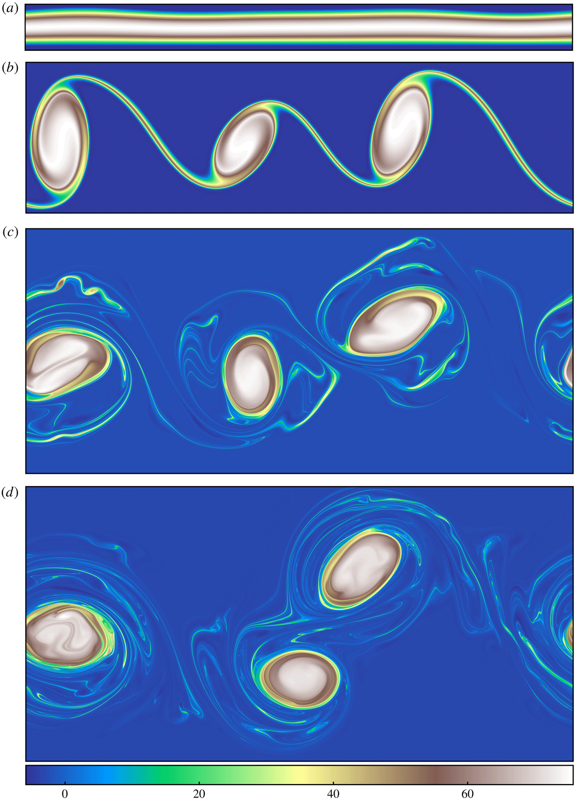
The initial ribbon of PV destabilises and rolls up into set of unequal-sized vortices. The evolution qualitatively resembles that exhibited by a strip of uniform PV in a two-dimensional (uniform depth) flow (Dritschel Reference Dritschel1989), and the instability arises from the phase locking and mutual amplification of the waves propagating on the PV contours. In the present case, two of the vortices formed at early times partially merge, leading to a rapid growth in complexity. The PV field develops exceedingly sharp gradients and a multitude of fine-scale filamentary debris. By the end of the simulation at
 $t=25$
, the flow becomes more regular, settling into a pair of dominant vortices. This is arguably a demanding test case for studying both GN and SW dynamics.
Divergence field
 $\unicode[STIX]{x1D6FF}$
at early times (as indicated) in both the GN and SW dynamics (top and bottom) starting from
 $\unicode[STIX]{x1D6FF}=\unicode[STIX]{x1D6FE}=0$
.

Divergence field
 $\unicode[STIX]{x1D6FF}$
at late times in both the GN and SW dynamics starting from
 $\unicode[STIX]{x1D6FF}=\unicode[STIX]{x1D6FE}=0$
.

Like PV, the fields of height
 $h$
, velocity
 $\boldsymbol{u}$
, vorticity
 $\unicode[STIX]{x1D701}$
and, to a lesser extent, acceleration divergence
 $\unicode[STIX]{x1D6FE}$
exhibit closely similar behaviour in the GN and SW simulations. The one field that stands out is the divergence
 $\unicode[STIX]{x1D6FF}$
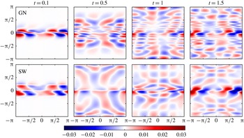
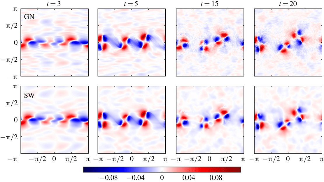
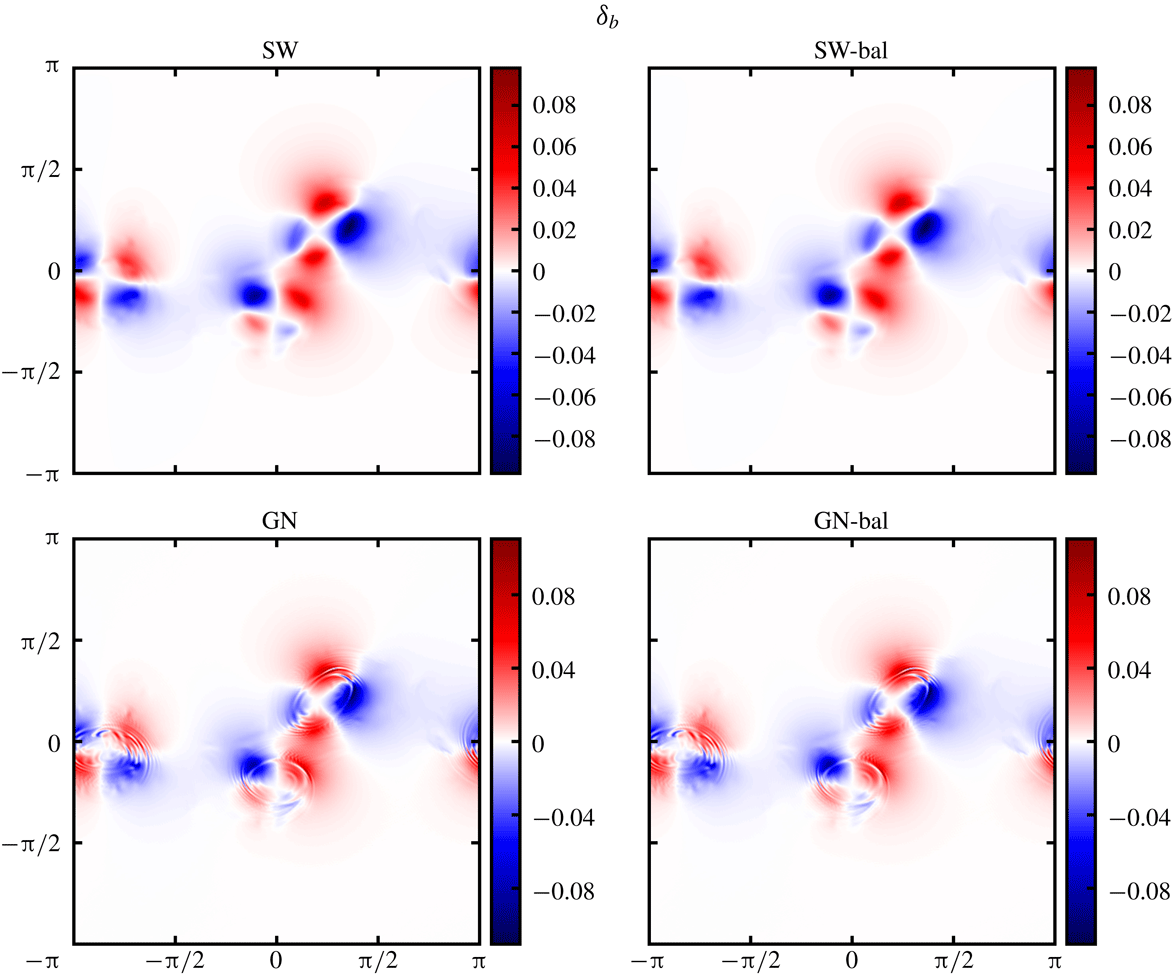
, shown in figure 2 at early times and in figure 3 at late times. The divergence largely consists of gravity waves generated by the imbalanced initial conditions (this is demonstrated below). These waves propagate differently in the GN and SW dynamics, due in part to a fundamental difference in the linear dispersion relation for waves on a basic state at rest. Considering small disturbances proportional to
 $\exp \text{i}(k_{x}x+k_{y}y-\unicode[STIX]{x1D714}t)$
, in the SW dynamics such waves have frequencies
 $$\begin{eqnarray}\displaystyle \unicode[STIX]{x1D714}=\pm \sqrt{f^{2}+c^{2}k^{2}}, & & \displaystyle\end{eqnarray}$$
where
 $c=\sqrt{gH}$
and
 $k=\sqrt{k_{x}^{2}+k_{y}^{2}}$
is the wavenumber magnitude. Hence, all gravity waves have phase speeds
 $c_{p}=\unicode[STIX]{x1D714}/k$
exceeding
 $c$
, with the longest waves having the highest speeds. Moreover, the group velocity
 $c_{g}=\Vert (\unicode[STIX]{x2202}\unicode[STIX]{x1D714}/\unicode[STIX]{x2202}k_{x},\unicode[STIX]{x2202}\unicode[STIX]{x1D714}/\unicode[STIX]{x2202}k_{y})\Vert \rightarrow c=\sqrt{gH}$
for
 $k_{x}\rightarrow \infty$
and/or
 $k_{y}\rightarrow \infty$
. Hence, short-scale waves propagate away from their source. However, in the GN dynamics, gravity waves propagate at the frequencies
 $$\begin{eqnarray}\displaystyle \unicode[STIX]{x1D714}=\pm \sqrt{\frac{f^{2}+c^{2}k^{2}}{1+{\textstyle \frac{1}{3}}H^{2}k^{2}}}. & & \displaystyle\end{eqnarray}$$
Here, short waves having wavelengths comparable to or less than
 $H$
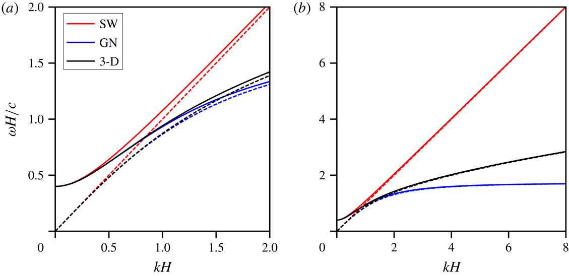
are slowed down relative to the SW dynamics (the GN and SW dispersion relations are compared in figure 16, which also includes the exact dispersion relation for a 3-D fluid derived in § 4). In fact the shortest waves have both vanishing phase and group velocities:
 $c_{p},\,c_{g}\rightarrow 0$
as
 $k_{x}\rightarrow \infty$
and/or
 $k_{y}\rightarrow \infty$
. This is responsible for the differences seen between the GN and SW divergence evolution in figures 2 and 3. In the GN dynamics, the short-scale gravity waves remain close to the centre of the domain in
 $y$
, whereas in the SW dynamics, all waves propagate away. In both dynamics, long waves escape most rapidly, re-entering the periodic edges and creating a complex interference pattern at late times.
Divergence field
 $\unicode[STIX]{x1D6FF}$
at
 $t=25$
in both SW and GN simulations starting from either
 $\unicode[STIX]{x1D6FF}=\unicode[STIX]{x1D6FE}=0$
or
 $\unicode[STIX]{x1D6FF}_{t}=\unicode[STIX]{x1D6FE}_{t}=0$
. The former simulations are denoted by SW and GN, while the latter are denoted by SW-bal and GN-bal.

In simulations initialised with the balance conditions
 $\unicode[STIX]{x1D6FF}_{t}=\unicode[STIX]{x1D6FE}_{t}=0$
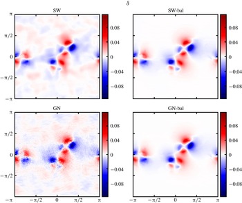
(see § 3.2 for details), the gravity waves are much weaker at all later times – even in the divergence field
 $\unicode[STIX]{x1D6FF}$
. This is shown in figure 4 comparing
 $\unicode[STIX]{x1D6FF}$
at
 $t=25$
between four simulations differing in the model used (SW or GN) and/or the initialisation used (
 $\unicode[STIX]{x1D6FF}=\unicode[STIX]{x1D6FE}=0$
or
 $\unicode[STIX]{x1D6FF}_{t}=\unicode[STIX]{x1D6FE}_{t}=0$
). In the simulations starting from balance, the flow surrounding the vortices which emerged from the earlier instability contains much weaker amplitude divergence than seen in the simulations starting from
 $\unicode[STIX]{x1D6FF}=\unicode[STIX]{x1D6FE}=0$
. Instead, the divergence is primarily trapped in the vicinity of the vortices, evidence that the divergence remains close to balance. The characteristic quadrupole pattern of balanced divergence is a typical feature of elliptically deformed vortices in SW flows (see below).
3.2 Balance–imbalance decomposition
We next look more carefully at the balance and imbalance present in both the SW and GN flows. To do this, the PV anomaly field
 $\tilde{q}$
is taken from a particular simulation at a given time and used to generate associated balanced fields denoted by a subscript ‘
 $b$
’, e.g.
 $\unicode[STIX]{x1D6FF}_{b}$
, from the balance conditions
 $\unicode[STIX]{x1D6FF}_{t}=\unicode[STIX]{x1D6FE}_{t}=0$
. Hence, the balance fields depend only on
 $\tilde{q}$
; that is, they are entirely determined by
 $\tilde{q}$
. The residual, imbalanced fields are denoted by a subscript ‘
 $i$
’, e.g.
 $\unicode[STIX]{x1D6FF}_{i}=\unicode[STIX]{x1D6FF}-\unicode[STIX]{x1D6FF}_{b}$
. These fields are regarded as gravity waves, though a precise definition of gravity waves in a nonlinear flow is impossible (Ford et al.
Reference Ford, McIntyre and Norton2000; Mohebalhojeh & Dritschel Reference Mohebalhojeh and Dritschel2001). Nonetheless, the definition of balance adopted adequately identifies plausible gravity waves in the flows simulated.
Numerically, the balanced fields are found by solving (C 1) and (C 2), with
 $\unicode[STIX]{x1D6FF}_{t}=\unicode[STIX]{x1D6FE}_{t}=0$
and no diffusion
 $\mathbb{D}=0$
, for
 $\unicode[STIX]{x1D6FF}$
and
 $\unicode[STIX]{x1D6FE}$
iteratively until convergence. At each step of the iteration, we must also recover the height
 $h$
and velocity fields
 $\boldsymbol{u}$
by the inversion procedure described in appendix A. Upon convergence, the fields obtained are denoted
 $h_{b}$
,
 $\boldsymbol{u}_{b}$
, etc.
In the SW dynamics, convergence is said to occur when
 $$\begin{eqnarray}\displaystyle \frac{\langle (\unicode[STIX]{x0394}\unicode[STIX]{x1D6FF})^{2}\rangle }{\langle \unicode[STIX]{x1D6FF}^{2}\rangle }+\frac{\langle (\unicode[STIX]{x0394}\unicode[STIX]{x1D6FE})^{2}\rangle }{\langle \unicode[STIX]{x1D6FE}^{2}\rangle }<2\times 10^{-10}, & & \displaystyle\end{eqnarray}$$
where
 $\unicode[STIX]{x0394}\unicode[STIX]{x1D6FF}$
and
 $\unicode[STIX]{x0394}\unicode[STIX]{x1D6FE}$
are the changes in
 $\unicode[STIX]{x1D6FF}$
and
 $\unicode[STIX]{x1D6FE}$
, respectively, between the last two estimates. In the GN dynamics, convergence is poorer and in particular cannot reach such low levels of error. Instead, the iteration with the smallest level of error is considered to be converged. This error can be as large as
 $10^{-4}$
. Moreover, to achieve even this level of convergence, it is first necessary to find the SW balanced fields and use them as a first guess in the iteration to find the GN ones. Otherwise, the error may be substantially larger. Suffice it to say, balance in the GN dynamics is much harder to achieve. This is an indication that the regularity of the GN equations is significantly poorer than that of the SW equations.
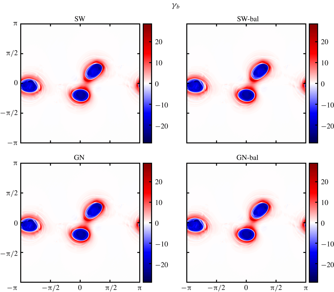
Balanced divergence field
 $\unicode[STIX]{x1D6FF}_{b}$
at
 $t=25$
in both SW and GN simulations starting from either
 $\unicode[STIX]{x1D6FF}=\unicode[STIX]{x1D6FE}=0$
or
 $\unicode[STIX]{x1D6FF}_{t}=\unicode[STIX]{x1D6FE}_{t}=0$
.

Consider then the balanced divergence fields
 $\unicode[STIX]{x1D6FF}_{b}$
in the SW and GN simulations at
 $t=25$
. These are shown in figure 5 and should be compared with the corresponding full fields in figure 4. First of all, note the absence of significant balanced divergence in the background flow far from the vortices. The balanced divergence is mainly concentrated around the vortices and exhibits a predominant quadrupole pattern in all simulations. In the GN simulations,
 $\unicode[STIX]{x1D6FF}_{b}$
further exhibits fine-scale structure concentrated where the PV gradients are strongest. Due to the peculiar gravity-wave dispersion relation in the GN equations (see (3.4)), this fine-scale structure could in fact be trapped gravity waves, since the group velocity
 $c_{g}\rightarrow 0$
for
 $k_{x}\rightarrow \infty$
and/or
 $k_{y}\rightarrow \infty$
. Hence, gravity waves generated by evolving sharp PV gradients cannot easily escape. By contrast, in the SW dynamics,
 $c_{g}\rightarrow c=\sqrt{gH}$
for short-scale waves, and hence such waves propagate away from their source. Note that, despite the different initial conditions used, the SW and SW-bal balanced fields are closely similar, as are the GN and GN-bal ones.
Imbalanced divergence field
 $\unicode[STIX]{x1D6FF}_{i}$
at
 $t=25$
in both SW and GN simulations starting from either
 $\unicode[STIX]{x1D6FF}=\unicode[STIX]{x1D6FE}=0$
or
 $\unicode[STIX]{x1D6FF}_{t}=\unicode[STIX]{x1D6FE}_{t}=0$
.

The corresponding imbalanced divergence fields
 $\unicode[STIX]{x1D6FF}_{i}$
are shown in figure 6. In the SW simulation, comparable amplitudes of
 $\unicode[STIX]{x1D6FF}_{i}$
are seen throughout the flow, with a slight increase in the generation region around the vortices. Nonetheless, the largest
 $\unicode[STIX]{x1D6FF}_{i}$
values are only approximately 20 % of the largest
 $\unicode[STIX]{x1D6FF}_{b}$
values. In the SW-bal simulation,
 $\unicode[STIX]{x1D6FF}_{i}$
is largest where it is being generated and weakens as it disperses throughout the domain. Amplitudes of
 $\unicode[STIX]{x1D6FF}_{i}$
are noticeably smaller than in the SW simulation. In the GN simulation,
 $\unicode[STIX]{x1D6FF}_{i}$
exhibits much more fine-scale structure than in the SW simulation, and at a much larger amplitude – comparable to
 $\unicode[STIX]{x1D6FF}_{b}$
. The largest amplitudes occur along the sharp PV gradients bounding each vortex; here the gravity waves are trapped, as discussed above. In the GN-bal simulation, there is much less fine-scale structure far from the vortices but comparable imbalance near the vortices. The pattern of
 $\unicode[STIX]{x1D6FF}_{i}$
is consistent with slowly propagating short-scale waves.
Balanced acceleration divergence field
 $\unicode[STIX]{x1D6FE}_{b}$
at
 $t=25$
in both SW and GN simulations starting from either
 $\unicode[STIX]{x1D6FF}=\unicode[STIX]{x1D6FE}=0$
or
 $\unicode[STIX]{x1D6FF}_{t}=\unicode[STIX]{x1D6FE}_{t}=0$
.

Imbalanced acceleration divergence field
 $\unicode[STIX]{x1D6FE}_{i}$
at
 $t=25$
in both SW and GN simulations starting from either
 $\unicode[STIX]{x1D6FF}=\unicode[STIX]{x1D6FE}=0$
or
 $\unicode[STIX]{x1D6FF}_{t}=\unicode[STIX]{x1D6FE}_{t}=0$
.

We briefly discuss the acceleration divergence
 $\unicode[STIX]{x1D6FE}$
as it is a primary variable in the reformulated equations. The balanced and imbalanced components,
 $\unicode[STIX]{x1D6FE}_{b}$
and
 $\unicode[STIX]{x1D6FE}_{i}$
respectively, are shown in figures 7 and 8 for all four simulations at the final time
 $t=25$
. Though not shown,
 $\unicode[STIX]{x1D6FE}$
is hardly distinguishable from
 $\unicode[STIX]{x1D6FE}_{b}$
, apart from some weak fine-scale structure in the GN simulations. The imbalance
 $\unicode[STIX]{x1D6FE}_{i}$
has much weaker amplitude, and resembles propagating gravity waves like those seen in
 $\unicode[STIX]{x1D6FF}_{i}$
in figure 6.
Residual acceleration divergence field
 $\tilde{\unicode[STIX]{x1D6FE}}$
(or quasi-geostrophic imbalance) at
 $t=25$
in both SW and GN simulations starting from either
 $\unicode[STIX]{x1D6FF}=\unicode[STIX]{x1D6FE}=0$
or
 $\unicode[STIX]{x1D6FF}_{t}=\unicode[STIX]{x1D6FE}_{t}=0$
.

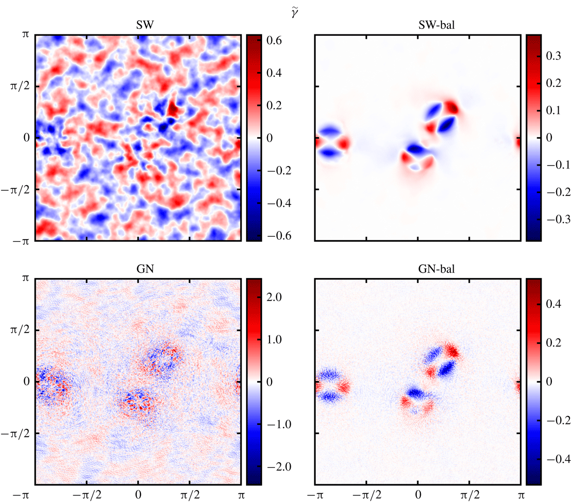
The acceleration divergence is mainly confined to the vortex cores and is strongly negative there. Notably,
 $\tilde{\unicode[STIX]{x1D6FE}}$
defined in (2.9) and shown in figure 9 is of much weaker amplitude and is significantly less well balanced than
 $\unicode[STIX]{x1D6FE}$
, or even
 $\unicode[STIX]{x1D6FF}$
. The condition
 $\tilde{\unicode[STIX]{x1D6FE}}=0$
may be regarded as ‘quasi-geostrophic balance’, as it is essentially the balance obtained at second order in Rossby number under quasi-geostrophic scaling (see Appendix A in Mohebalhojeh & Dritschel Reference Mohebalhojeh and Dritschel2001), namely
 $\unicode[STIX]{x1D6FE}+2J(u,v)=0$
. Since
 $\unicode[STIX]{x1D6FF}$
is already second order in Rossby number under this scaling, then the extra
 $2\unicode[STIX]{x1D6FF}^{2}$
term in
 $\tilde{\unicode[STIX]{x1D6FE}}\equiv \unicode[STIX]{x1D6FE}+2J(u,v)-2\unicode[STIX]{x1D6FF}^{2}$
makes no difference at this order. Note, this balance is sometimes referred to as cyclostrophic or gradient-wind balance in the literature.
Like divergence,
 $\tilde{\unicode[STIX]{x1D6FE}}$
exhibits a quadrupole pattern around each vortex, but the pattern is rotated by
 $45^{\circ }$
. This is particularly evident in the SW and GN simulations starting from balance. The other simulations are dominated by imbalance, which is intermediate scale in the SW simulation and fine scale in the GN simulation. Finally, note that
 $\tilde{\unicode[STIX]{x1D6FE}}$
is significantly different from
 $\unicode[STIX]{x1D6FE}_{i}$
, even though they often have closely comparable amplitudes.
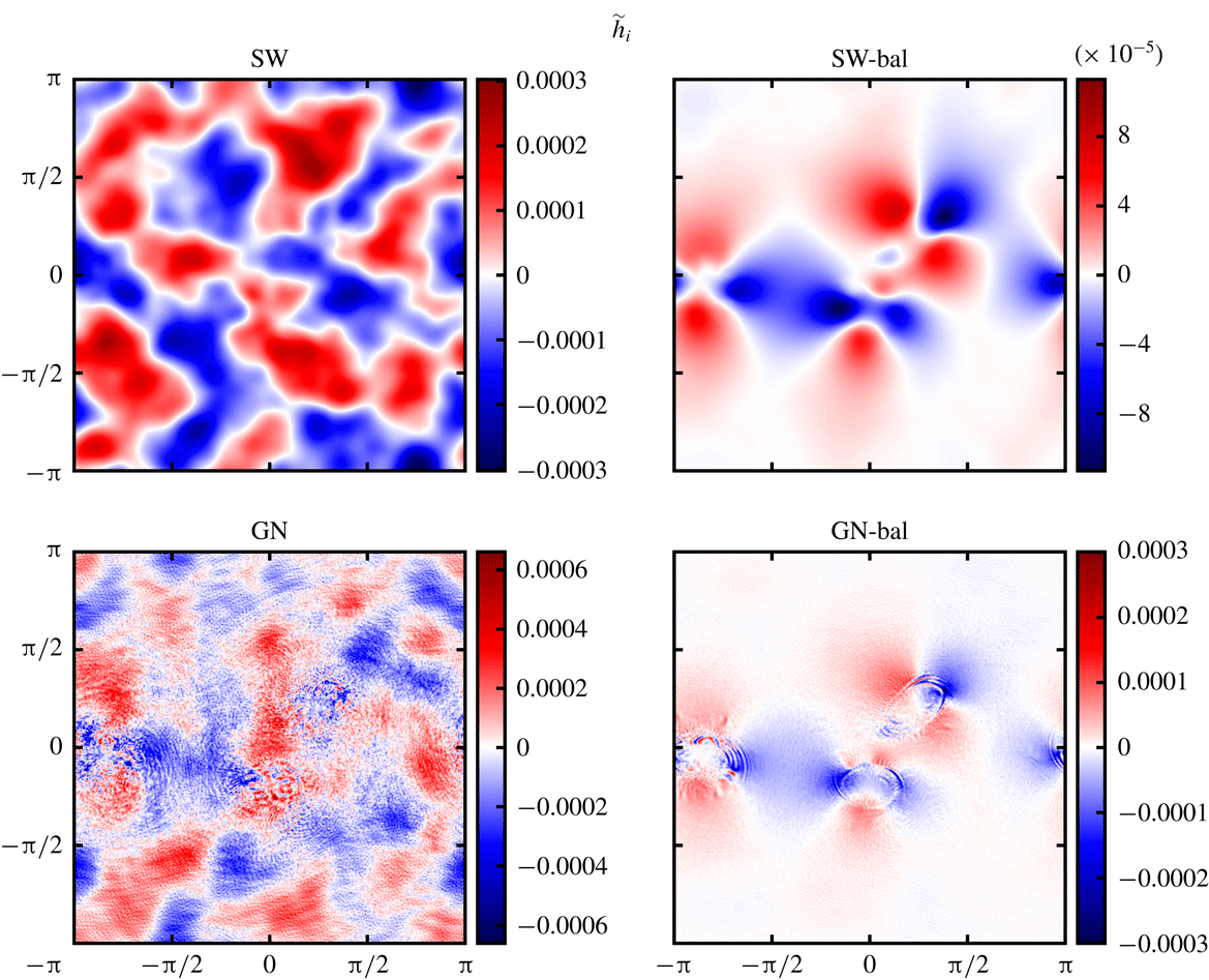
Imbalanced height anomaly field
 $\tilde{h}_{i}$
at
 $t=25$
in both SW and GN simulations starting from either
 $\unicode[STIX]{x1D6FF}=\unicode[STIX]{x1D6FE}=0$
or
 $\unicode[STIX]{x1D6FF}_{t}=\unicode[STIX]{x1D6FE}_{t}=0$
.

The height anomaly field
 $\tilde{h}$
exhibits the greatest degree of balance, and the differences between the four simulations are imperceptible. However, the structure of the imbalanced fields
 $\tilde{h}_{i}$
is revealing, as shown in figure 10. First of all, the amplitudes are around a thousand times smaller than the amplitude of
 $\tilde{h}$
, or even smaller in the SW-bal simulation. The imbalance is predominantly at large scales in the SW simulations, but exists at both small and large scales in the GN simulations, with the largest amplitudes concentrated in the smallest features. Gravity waves appear to be trapped on the edges of the vortices in the GN simulations, most clearly in the GN-bal simulation (the same is seen in the fields of
 $\unicode[STIX]{x1D6FF}_{i}$
and
 $\unicode[STIX]{x1D6FE}_{i}$
).
The differences between the SW and GN solutions mainly arise from the additional terms in the GN equation relating
 $\tilde{h}$
to
 $\unicode[STIX]{x1D6FF}$
,
 $\unicode[STIX]{x1D6FE}$
and
 $q$
, see (2.20) or (A 3). The terms multiplied by
 $1/3$
in (2.20) are all absent in the corresponding SW equation. These terms may reduce the regularity of
 $\tilde{h}$
(make it less differentiable) since both
 $\unicode[STIX]{x1D6FF}$
and
 $\unicode[STIX]{x1D6FE}$
are differentiated on the right-hand side. In the next subsection, we verify this by considering field spectra.
Root-mean-square (r.m.s.) norms of the balanced fields
 $h_{b}$
,
 $\unicode[STIX]{x1D701}_{b}$
,
 $\unicode[STIX]{x1D6FF}_{b}$
and
 $\unicode[STIX]{x1D6FE}_{b}$
as a function of time in both SW and GN simulations starting from either
 $\unicode[STIX]{x1D6FF}=\unicode[STIX]{x1D6FE}=0$
or
 $\unicode[STIX]{x1D6FF}_{t}=\unicode[STIX]{x1D6FE}_{t}=0$
.

Root-mean-square norms of the imbalanced fields
 $h_{i}$
,
 $\unicode[STIX]{x1D701}_{i}$
,
 $\unicode[STIX]{x1D6FF}_{i}$
and
 $\unicode[STIX]{x1D6FE}_{i}$
as a function of time in both SW and GN simulations starting from either
 $\unicode[STIX]{x1D6FF}=\unicode[STIX]{x1D6FE}=0$
or
 $\unicode[STIX]{x1D6FF}_{t}=\unicode[STIX]{x1D6FE}_{t}=0$
.

The time evolution of the root-mean-square (r.m.s.) values of the balanced and imbalanced fields are summarised in figures 11 and 12, for all four simulations. The balanced norms are closely similar, despite the differences in the initial conditions and model type (SW or GN). Only
 $h_{b}$
and
 $\unicode[STIX]{x1D6FF}_{b}$
show slight differences emerging after
 $t=6$
. Moreover, the GN results are rougher, an indication of the increased power at small scales in the GN simulations. On the other hand, the imbalanced norms show wide variations, with the closest results found between SW-bal and GN-bal, apart from
 $\unicode[STIX]{x1D6FF}_{i}$
, which is approximately 3 times larger in the GN-bal simulation. The results for SW and GN are rougher and reflect the significant gravity-wave activity released initially from the imbalanced initial conditions. Here,
 $\unicode[STIX]{x1D6FF}_{i}$
in GN is about 2 times larger than in SW, while
 $\unicode[STIX]{x1D6FE}_{i}$
in GN starts initially comparable to that in SW but eventually also becomes 2 times larger. The spike around
 $t=22$
in the GN-bal results is the result of poor convergence of the post-processing balancing routine. This also explains the rise in
 $\unicode[STIX]{x1D6FF}_{i}$
and
 $\unicode[STIX]{x1D6FE}_{i}$
after
 $t=23$
.
3.3 Spectra
To better understand the differences between the SW and GN simulations, we turn next to the power spectra of various fields. The power spectrum of
 $h$
, for example, is defined by
 $$\begin{eqnarray}\displaystyle S_{h}(k)=\mathop{\sum }_{k_{x},k_{y}\in R(k)}|{\hat{h}}(k_{x},k_{y})|^{2}, & & \displaystyle\end{eqnarray}$$
where
 ${\hat{h}}(k_{x},k_{y})$
is the Fourier coefficient for the wave vector
 $(k_{x},k_{y})$
and
 $R(k)$
is the set of all wave vectors lying in the shell
 $k-1/2\leqslant \sqrt{k_{x}^{2}+k_{y}^{2}}<k+1/2$
. The power spectrum thus measures the contribution of each length scale
 $2\unicode[STIX]{x03C0}/k$
to the mean-square field amplitude
 $\langle h^{2}\rangle$
.
Power spectra of the original fields
 $h$
,
 $\unicode[STIX]{x1D701}$
,
 $\unicode[STIX]{x1D6FF}$
and
 $\unicode[STIX]{x1D6FE}$
at
 $t=25$
for both SW and GN simulations starting from either
 $\unicode[STIX]{x1D6FF}=\unicode[STIX]{x1D6FE}=0$
or
 $\unicode[STIX]{x1D6FF}_{t}=\unicode[STIX]{x1D6FE}_{t}=0$
. The vertical dashed line corresponds to the wavenumber
 $k=3/H$
.

Spectra of the original fields
 $h$
,
 $\unicode[STIX]{x1D701}$
,
 $\unicode[STIX]{x1D6FF}$
and
 $\unicode[STIX]{x1D6FE}$
are shown in figure 13 at
 $t=25$
for all four simulations (note the
 $\log _{10}$
scaling of both axes). The vertical dashed line in the plots marks the wavenumber
 $k=3/H$
where the frequency of gravity waves in GN is reduced by a factor of two relative to that in SW (see (3.3) and (3.4)). First of all, the vorticity spectra are practically indistinguishable. This means that the non-divergent part of the flow is closely similar in all simulations, and is insensitive to any imbalance present. The acceleration divergence spectra also correspond, apart from that in the GN simulation at small scales (
 $\log _{10}k>1.9$
). This heightened activity at small scales is especially visible in figure 9 for
 $\tilde{\unicode[STIX]{x1D6FE}}$
(which mainly differs from
 $\unicode[STIX]{x1D6FE}$
by
 $2J(u,v)$
).
The height spectra closely correspond at large and intermediate scales (
 $\log _{10}k<1.5$
), but again the GN simulation shows much greater power at small scales. Even the GN-bal simulation shows increased power, but it is approximately 100 times smaller than in the GN one. The fact that spectra flatten or even rise (in the GN simulation) at high
 $k$
is not a numerical artefact: numerical damping does not appreciably change the spectra except near
 $k=n/2$
(or
 $\log _{10}k=2.408\ldots$
). The flat or rising spectra indicate a fundamental problem in the GN equations: their representation of small scales. To represent these scales, fields should converge with increasing resolution, and the present results indicate this does not happen for
 $h$
. Simulations performed at
 $n=256$
resolution reveal the same problem to a lesser degree:
 $h$
spectra flatten but do not rise toward
 $k=n/2$
(not shown). Increasing resolution does not solve the problem – it makes it worse. This is reflected in the poor convergence of total energy discussed in the next subsection.
Finally, divergence spectra show the greatest differences between the SW and GN simulations. A broader range of scales show increased power in GN, and even in GN-bal. The SW and SW-bal spectra are indistinguishable across all scales. The GN and SW spectra separate around the wavenumber
 $k=3/H$
where the gravity-wave frequencies in the two models differ by a factor of two. The other significant difference between the SW and GN simulations occurs at large scales, and only for
 $\unicode[STIX]{x1D6FF}$
. Evidently, the additional nonlinear terms in the GN equations contribute to divergence at large scales as well as at small scales.
The nearly flat spectra seen in both
 $h$
and
 $\unicode[STIX]{x1D6FF}$
in the GN simulations at large
 $k$
are problematic for the regularity of the GN equations. If a quantity
 $a$
has a spectrum
 $S_{a}\sim k^{-p}$
for large
 $k$
, the corresponding Fourier amplitudes scale as
 $|\hat{a}|^{-(1+p)/2}$
. Both
 $S_{h}$
and
 $S_{\unicode[STIX]{x1D6FF}}$
decay more slowly than
 $k^{-1}$
, implying that both
 $|{\hat{h}}|$
and
 $|\hat{\unicode[STIX]{x1D6FF}}|$
also decay more slowly than
 $k^{-1}$
. This means that derivatives of
 $h$
and
 $\unicode[STIX]{x1D6FF}$
do not converge with increasing resolution. But in the GN equations as originally formulated, three derivatives of
 $h$
appear in the non-hydrostatic pressure term in (2.1). For this to be resolvable,
 $|{\hat{h}}|$
would have to decay faster than
 $k^{-3}$
and the spectrum
 $S_{h}$
would have to decay faster than
 $k^{-5}$
. This is not observed, and seriously questions the mathematical regularity of the GN equations. By contrast, only one derivative of
 $h$
or of
 $\boldsymbol{u}$
appears in the SW equations, and all spectra are sufficiently steep that these derivatives converge with increasing resolution.
Power spectra of the imbalanced fields
 $h_{i}$
,
 $\unicode[STIX]{x1D701}_{i}$
,
 $\unicode[STIX]{x1D6FF}_{i}$
and
 $\unicode[STIX]{x1D6FE}_{i}$
at
 $t=25$
for both SW and GN simulations starting from either
 $\unicode[STIX]{x1D6FF}=\unicode[STIX]{x1D6FE}=0$
or
 $\unicode[STIX]{x1D6FF}_{t}=\unicode[STIX]{x1D6FE}_{t}=0$
. The vertical dashed line corresponds to the wavenumber
 $k=3/H$
.

Further differences are revealed by examining the spectra of the imbalanced fields
 $h_{i}$
,
 $\unicode[STIX]{x1D701}_{i}$
,
 $\unicode[STIX]{x1D6FF}_{i}$
and
 $\unicode[STIX]{x1D6FE}_{i}$
. Figure 14 shows that while SW spectra rapidly decay with increasing
 $k$
, the GN spectra are either flat or rising, indicating that the GN equations are incapable of representing small-scale imbalance. Again, the problem is exacerbated at high resolutions, as confirmed by examining spectra at lower resolution (not shown). The shallow GN spectra reflect the grainy appearance seen in the GN imbalanced fields in figures 6, 8 and 10. The GN and SW spectra separate even before the wavenumber
 $k=3/H$
where the gravity wave frequencies in the two models differ by a factor of two. Only the largest wavenumbers approximately correspond.
3.4 Energy
Another important, and revealing, diagnostic is the energy per unit mass
 ${\mathcal{E}}={\mathcal{H}}/H$
, see (2.21), which is conserved in the absence of forcing and dissipation. This energy may be divided into kinetic
 ${\mathcal{K}}$
and (available) potential
 ${\mathcal{P}}$
parts, defined by
 $$\begin{eqnarray}\displaystyle & \displaystyle {\mathcal{K}}=\frac{A}{2}\langle (1+\tilde{h})\Vert \boldsymbol{u}\Vert ^{2}\rangle +\frac{AH^{2}}{6}\langle (1+\tilde{h})^{3}\unicode[STIX]{x1D6FF}^{2}\rangle , & \displaystyle\end{eqnarray}$$
 $$\begin{eqnarray}\displaystyle & \displaystyle {\mathcal{P}}=\frac{Ac^{2}}{2}\langle \tilde{h}^{2}\rangle , & \displaystyle\end{eqnarray}$$
where
 $A$
is the domain area (
 $A=4\unicode[STIX]{x03C0}^{2}$
) and
 $c^{2}=gH$
. The potential energy excludes the constant mean part
 $Ac^{2}/2$
, which is not available dynamically for exchange with the kinetic energy. In the SW model, the second term in
 ${\mathcal{K}}$
is absent.
Evolution of the kinetic
 ${\mathcal{K}}$
, potential
 ${\mathcal{P}}$
and total energy
 ${\mathcal{E}}={\mathcal{K}}+{\mathcal{P}}$
at two resolutions:
 $n=512$
(a–c) and
 $n=256$
(d–f). Results are presented for both SW and GN simulations starting from either
 $\unicode[STIX]{x1D6FF}=\unicode[STIX]{x1D6FE}=0$
or
 $\unicode[STIX]{x1D6FF}_{t}=\unicode[STIX]{x1D6FE}_{t}=0$
.

Figure 15 shows the evolution of
 ${\mathcal{K}}$
,
 ${\mathcal{P}}$
and
 ${\mathcal{E}}={\mathcal{K}}+{\mathcal{P}}$
for all four simulations and at two different resolutions:
 $n=512$
(a–c) and
 $n=256$
(d–f). Both
 ${\mathcal{K}}$
and
 ${\mathcal{P}}$
exhibit variations of the order of 0.1 and smaller high-frequency variations (associated with gravity waves) which approximately cancel out. The total energy is conserved to within a few tenths of a per cent and does not exhibit high-frequency variations.
The initially balanced simulations SW-bal and GN-bal have a little less energy than their imbalanced counterparts, and this energy difference remains approximately constant in time. The loss in energy is not due to dissipating gravity waves, though there is some effect of hyperdiffusion. There are many more gravity waves present in the SW and GN simulations, and these waves persist. Instead, the loss in energy is caused by the dissipation of a multitude of PV filaments following the roll-up of the initial ribbon of PV into vortices, see figure 1. The loss of energy can be reduced primarily by reducing the hyperdiffusion acting on the residual PV in the numerical method used (see appendix C), but this comes at a price: field spectra at high wavenumbers then show a strong upturn due to insufficient damping (not shown). The energy loss seen is an inevitable consequence of finite resolution.
More important is how the energy loss changes with resolution
 $n$
. First consider the SW simulations. For
 $n=256$
, the energy loss over
 $0\leqslant t\leqslant 25$
is approximately
 $0.004274$
, while for
 $n=512$
, the loss is approximately 0.001007 (in both SW and SW-bal). The error thus reduces by a factor of 3.995, compatible with an energy spectrum decaying like
 $k^{-3}$
for large
 $k$
. This spectrum is expected for a strong PV filament cascade to small scales in the flow regime considered (Dritschel et al.
Reference Dritschel, Scott, Macaskill, Gottwald and Tran2009). Qualitatively, the unresolved energy in wavenumbers
 $k\geqslant n/2$
is proportional to
 $$\begin{eqnarray}\displaystyle \int _{n/2}^{\infty }k^{-3}\propto n^{-2}. & & \displaystyle\end{eqnarray}$$
Thus, a doubling of resolution should reduce the total energy loss by a factor of
 $4$
, as observed in the SW simulations.
Next consider the GN simulations. For
 $n=256$
, the energy loss over the same time period is about 0.005816, while for
 $n=512$
, the loss is about 0.003203 (in both GN and GN-bal). The error reduces by a factor of 1.816, which is much less than the factor of 3.995 found for the SW simulations (and corresponds to a spectral decay close to
 $k^{-7/3}$
). This poor convergence comes from the enhanced, and likely spurious, small-scale activity in the GN simulations, seen already in the field spectra in figure 13. The likely contributors are the height
 $h$
and divergence
 $\unicode[STIX]{x1D6FF}$
, whose spectra are greatly enhanced at small scales relative to those found in the SW simulations. Vorticity spectra are equally steep and closely similar in all simulations. This means that the divergent part of the velocity field dominates the kinetic energy at small scales (compounded by the poor behaviour of
 $h$
). The potential energy likewise is affected by the behaviour of
 $h$
at small scales, leading to stronger dissipation. In summary, the erroneous fine-scale structure in the height and divergence fields is responsible for the poor convergence of the GN simulations.
3.5 Parameter variations
This study has focused on a particular flow to enable a careful assessment of the differences between GN and SW flows. However, the differences reported are not unique to the particular flow considered. We have also examined increasing
 $H$
from 0.2 to 0.3 or reducing it to 0.1, and the primary impact of this is to shift the transition wavenumber
 $k=3/H$
where GN divergence spectra and all imbalance spectra separate from the corresponding SW spectra. On the other hand, halving
 $c$
greatly slows down the dynamics, since the Rossby deformation length
 $L_{D}$
is reduced by two, and this length controls the range of interaction between different parts of the flow. Increasing the PV in the initial ribbon increases both the Rossby and Froude numbers, making the flow evolve more rapidly and in a more nonlinear manner, with stronger imbalance. All of these effects, apart from
 $H$
, are well known in past SW studies (see e.g. Polvani et al.
Reference Polvani, McWilliams, Spall and Ford1994; Płotka & Dritschel Reference Płotka and Dritschel2014). They do not qualitatively affect the differences observed between GN and SW flows. Those differences occur primarily at small scales, except for the divergence, which differs at all scales. In the following section, we explain why these differences are likely to be erroneous.
4 Conclusions
For shallow flows, the Green–Naghdi model (Serre Reference Serre1953; Green & Naghdi Reference Green and Naghdi1976a ) is widely considered to be a more accurate extension of the classical shallow-water model. Both models are founded on the assumption that the horizontal flow is independent of depth (Miles & Salmon Reference Miles and Salmon1985), but the shallow-water model goes further and imposes the hydrostatic approximation. This greatly simplifies the model, at the expense of a less accurate representation of linear wave dispersion.
The Green–Naghdi equations are implicit and challenging to solve numerically. In the present work, we find that the computational cost is approximately three times greater than required for the shallow-water equations. Higher-level Green–Naghdi equations exist (Shields & Webster Reference Shields and Webster1988), but their exceedingly complex form makes their study impractical.
Regardless, this study has exposed a fundamental and serious shortcoming of the Green–Naghdi model. The model fails to properly represent nonlinear interactions at small scales, likely leading to a lack of regularity of the mathematical equations. This is seen not only in the grainy appearance of the divergence field
 $\unicode[STIX]{x1D735}\boldsymbol{\cdot }\boldsymbol{u}$
in particular, but also in field spectra, including that of the height field
 $h$
. Consequently, the numerical dissipation of energy is much greater in the Green–Naghdi model than in the shallow-water one, and convergence with resolution is poor (or even lacking for some fields).
The numerical evidence here, obtained using a carefully designed numerical algorithm, indicates that the spatial derivatives appearing in the original (momentum-based) Green–Naghdi equations do not converge with increasing resolution. In particular, the shallow height spectra observed indicate that not even one spatial derivative converges. But in fact three are needed to evaluate the non-hydrostatic pressure term appearing in the Green–Naghdi momentum equation. By contrast, the shallow-water equations exhibit sufficiently steep spectra (for the flow regime investigated here) to ensure convergence of all terms in the equations.
Shallow spectra do not, in themselves, imply a lack of regularity of the equations under consideration. The structure of the equations also matters. For example, the three-dimensional rotating stratified Boussinesq equations have been reported to exhibit energy spectra having a
 $-5/3$
slope at high wavenumbers (as in homogeneous turbulence, see Waite & Bartello Reference Waite and Bartello2006; Deusebio, Vallgren & Lindborg Reference Deusebio, Vallgren and Lindborg2013), indicating a forward energy cascade to progressively smaller scales. However, in the range of scales unaffected by dissipation, the corresponding spectral decay of the density and velocity fields is still sufficiently fast that the first spatial derivatives of these fields converge with increasing resolution (assuming existence of solutions). Notably, only first derivatives are required in the momentum-based formulation of these equations (excluding dissipation terms).
One may argue that dissipation is essential to regularise equations like Green–Naghdi or even shallow water in the high Froude number regime where shocks may form. Any system of fluid equations exhibiting a forward energy cascade needs a dissipation mechanism to remove that energy near the smallest scale resolved. In applications to geophysical fluid dynamics, the range of scales unaffected by dissipation is vast, well beyond present modelling capabilities. Instead, some sort of turbulent mixing argument is used to justify dissipating the smallest resolved scales just enough to prevent energy from building up there. With increasing resolution, one hopes that spectra converge, as for example seen in studies of three-dimensional rotating stratified flows (e.g. Waite & Bartello Reference Waite and Bartello2006; Deusebio et al.
Reference Deusebio, Vallgren and Lindborg2013). But for the Green–Naghdi equations, the situation appears to be fundamentally different. Spectra in the range of wavenumbers
 $k>1/H$
do not converge with increasing resolution. Even if viscous dissipation were included, this would only reduce spectral amplitudes for
 $k\gg 1/H$
, potentially leaving a wide range of wavenumbers unaffected by dissipation. Moreover, this range increases with resolution. This lack of convergence indicates that the equations lack regularity.
We argue that the assumption underpinning the derivation of the Green–Naghdi model for shallow flows, namely that the horizontal flow is independent of depth, does not properly represent motions at horizontal scales comparable to or less than the fluid depth. This is despite the fact that linear wave dispersion appears to be much better represented than in the shallow-water model (see below).
Basically, short-scale waves on a free surface are not typically associated with depth-independent fluid motions. More naturally, fluid motions decay with depth, as can be seen by considering the characteristics of linear waves in a homogeneous rotating three-dimensional fluid with a free surface. Taking the mean depth to be
 $H$
and the free surface to be at
 $z=H+\unicode[STIX]{x1D702}(x,y,t)$
with
 $\unicode[STIX]{x1D702}\ll H$
, the linearised equations of motion for a basic state at rest (in a rotating frame of reference) are
 $$\begin{eqnarray}\displaystyle & \displaystyle u_{t}-fv=-P_{x}^{\prime }, & \displaystyle\end{eqnarray}$$
 $$\begin{eqnarray}\displaystyle & \displaystyle v_{t}+fu=-P_{y}^{\prime }, & \displaystyle\end{eqnarray}$$
 $$\begin{eqnarray}\displaystyle & \displaystyle w_{t}=-P_{z}^{\prime }, & \displaystyle\end{eqnarray}$$
 $$\begin{eqnarray}\displaystyle & \displaystyle u_{x}+v_{y}+w_{z}=0, & \displaystyle\end{eqnarray}$$
where
 $P^{\prime }=p^{\prime }/\unicode[STIX]{x1D70C}$
is the perturbation pressure scaled by the density
 $\unicode[STIX]{x1D70C}$
, and
 $f/2$
is the background rotation rate. The boundary conditions are
 $$\begin{eqnarray}\displaystyle & \displaystyle w(x,y,0,t)=0, & \displaystyle\end{eqnarray}$$
 $$\begin{eqnarray}\displaystyle & \displaystyle w(x,y,H,t)=\unicode[STIX]{x1D702}_{t}, & \displaystyle\end{eqnarray}$$
 $$\begin{eqnarray}\displaystyle & \displaystyle P^{\prime }(x,y,H,t)=g\unicode[STIX]{x1D702} & \displaystyle\end{eqnarray}$$
(assuming there are no boundaries in
 $x$
and
 $y$
, or periodic ones). Seeking solutions of the form
 $$\begin{eqnarray}\displaystyle u(x,y,z,t)=\hat{u} (z)\text{e}^{\text{i}(k_{x}x+k_{y}y-\unicode[STIX]{x1D714}t)},\quad \text{etc.}, & & \displaystyle\end{eqnarray}$$
we find after straightforward algebra that
 $$\begin{eqnarray}\displaystyle {\hat{w}}_{zz}-\frac{\unicode[STIX]{x1D714}^{2}k^{2}}{\unicode[STIX]{x1D714}^{2}-f^{2}}{\hat{w}}=0, & & \displaystyle\end{eqnarray}$$
where
 $k^{2}=k_{x}^{2}+k_{y}^{2}$
is the squared horizontal wavenumber. The general solution consistent with
 ${\hat{w}}=0$
at
 $z=0$
is
 $$\begin{eqnarray}\displaystyle {\hat{w}}=A\sinh \left(\frac{\unicode[STIX]{x1D714}kz}{\sqrt{\unicode[STIX]{x1D714}^{2}-f^{2}}}\right), & & \displaystyle\end{eqnarray}$$
where
 $A$
is an arbitrary constant, and assuming
 $\unicode[STIX]{x1D714}^{2}>f^{2}$
. The scaled pressure perturbation has the form
 $$\begin{eqnarray}\displaystyle \hat{P}=\text{i}A\frac{\sqrt{\unicode[STIX]{x1D714}^{2}-f^{2}}}{k}\cosh \left(\frac{\unicode[STIX]{x1D714}kz}{\sqrt{\unicode[STIX]{x1D714}^{2}-f^{2}}}\right). & & \displaystyle\end{eqnarray}$$
Imposing the remaining boundary conditions leads to the dispersion relation
 $$\begin{eqnarray}\displaystyle \unicode[STIX]{x1D714}\sqrt{\unicode[STIX]{x1D714}^{2}-f^{2}}=gk\tanh \left(\frac{\unicode[STIX]{x1D714}kH}{\sqrt{\unicode[STIX]{x1D714}^{2}-f^{2}}}\right), & & \displaystyle\end{eqnarray}$$
which reduces to the well-known form
 $\unicode[STIX]{x1D714}^{2}=gk\tanh (kH)$
when
 $f=0$
, as well as to the shallow-water dispersion relation
 $\unicode[STIX]{x1D714}^{2}=f^{2}+gHk^{2}$
in the long-wave limit
 $kH\ll 1$
(see figure 16 for a comparison with the shallow-water and Green–Naghdi dispersion relations). The important point is that the horizontal velocity components, which have the form
 $$\begin{eqnarray}\displaystyle & \displaystyle \hat{u} =\frac{\unicode[STIX]{x1D714}k_{x}+\text{i}fk_{y}}{\unicode[STIX]{x1D714}^{2}-f^{2}}\hat{P}, & \displaystyle\end{eqnarray}$$
 $$\begin{eqnarray}\displaystyle & \displaystyle \hat{v}=\frac{\unicode[STIX]{x1D714}k_{y}-\text{i}fk_{x}}{\unicode[STIX]{x1D714}^{2}-f^{2}}\hat{P}, & \displaystyle\end{eqnarray}$$
vary with
 $z$
just like
 $\hat{P}$
. Only in the long-wave limit does
 $\hat{P}$
become independent of
 $z$
. This is the limit taken for the validity of the shallow-water equations.
Scaled dispersion relations (
 $\unicode[STIX]{x1D714}H/c$
versus
 $kH$
) for linear waves in the shallow-water (SW), Green–Naghdi (GN) and exact 3-D Euler equations (see § 3.1), with and without rotation (solid and dashed lines respectively) for the simulation parameters chosen. The figure on the left shows a zoom of the one on the right for
 $kH\leqslant 2$
. Note that the Green–Naghdi dispersion relation well approximates the exact relation in this range of wavenumbers. Only for
 $kH\gg 1$
does the Green–Naghdi relation underestimate the exact relation.

The Green–Naghdi equations appear to represent horizontal waves of arbitrary scale, but they do so incorrectly as just demonstrated. Shorter waves are not depth independent, yet this is the fundamental assumption from which the equations are derived (Miles & Salmon Reference Miles and Salmon1985). This is where the problem lies. A different starting assumption is required, one which couples horizontal and vertical variations. For example, one could use the linearised eigenmodes above, together with the zero-frequency mode corresponding to material conservation of potential vorticity, as a basis for the nonlinear equations. In this way, the linearised equations are guaranteed to have the correct dispersion relation, which the original Green–Naghdi equations only approximate. Nonlinear equations may be constructed by projecting the nonlinear terms onto the appropriate vertical basis functions (as given above). This has to be done in the spectral domain horizontally, and likely gives rise to integro-differential equations in the spatial domain.
The approach suggested above is similar in spirit to the one used for the Green–Naghdi equations, in that only one vertical mode – the gravest – is retained in order to derive a two-dimensional flow model. The parent Euler equations however allow for arbitrary vertical variations, so restricting the dynamics to only one mode is an approximation (though a commonly made one). Higher-order vertical modes may be accounted for along the same lines used to derive the higher-level Green–Naghdi equations (Shields & Webster Reference Shields and Webster1988; Demirbilek & Webster Reference Demirbilek and Webster1999), though these equations become exceedingly complicated beyond the 1st level. Arguably, accounting for the gravest vertical mode exactly in linear theory may lead to a significant advance in our understanding of shallow free-surface flows. At the very least, any model derived should exhibit regularity and possess a variational formulation to guarantee basic conservation. We hope to report on a new model in the near future.
To the authors’ knowledge, there have been no direct comparisons between the parent 3-D Euler equations for shallow free-surface flows and reduced two-dimensional equations, either shallow water or Green–Naghdi. While there have been many studies of 3-D Euler (or Navier–Stokes) flows with or without stratification in triply periodic geometry, they are not directly relevant to understanding a shallow flow, with energy dominantly residing at large scales (
 $kH<1$
), and having a free surface. The large scales in such flows are highly constrained by the shallow fluid depth, leading to qualitatively different dynamics and different nonlinear interactions between large and small scales, compared to those occurring in isotropic domains. The study of such shallow flows is a priority. It would allow one to accurately quantify the extent to which reduced models capture the dynamics of the parent equations – under conditions where one may expect a correspondence.
Appendix A. Numerical inversion procedure
Here we provide details on how we solve for
 $h$
,
 $u$
and
 $v$
given the variables
 $q$
,
 $\unicode[STIX]{x1D6FF}$
and
 $\unicode[STIX]{x1D6FE}$
. Following Dritschel et al. (Reference Dritschel, Gottwald and Oliver2017) (see § 4.2 therein), we scale the height field
 $h$
by the mean fluid depth
 $H$
and work with a dimensionless anomaly
 $\tilde{h}$
:
 $$\begin{eqnarray}\displaystyle h=H(1+\tilde{h}). & & \displaystyle\end{eqnarray}$$
The mean fluid depth remains constant due to mass conservation. Defined this way, the mean value of
 $\tilde{h}$
is zero.
Likewise, we work with the PV anomaly defined by
 $$\begin{eqnarray}\displaystyle \tilde{q} & = & \displaystyle Hq-f\nonumber\\ \displaystyle & = & \displaystyle \frac{\unicode[STIX]{x1D701}+f}{1+\tilde{h}}-f+\frac{H^{2}}{3}J(\tilde{h},\unicode[STIX]{x1D6FF}).\end{eqnarray}$$
This is zero for a flow at rest and with an undisturbed free surface. Since both
 $H$
and
 $f$
are constant, material conservation of
 $q$
implies the same for
 $\tilde{q}$
. In general, the mean value of
 $\tilde{q}$
, denoted
 $\overline{\tilde{q}}$
, is non-zero.
Letting
 $c^{2}\equiv gH$
be a characteristic squared gravity-wave speed, the dimensionless height anomaly
 $\tilde{h}$
is determined from (2.20), which becomes
 $$\begin{eqnarray}\displaystyle c^{2}\unicode[STIX]{x1D6FB}^{2}\tilde{h}-f(f+\tilde{q})\tilde{h}=f\tilde{q}-\unicode[STIX]{x1D6FE}-fA+\unicode[STIX]{x1D6FB}^{2}(B(1+\tilde{h}))+\unicode[STIX]{x1D735}\boldsymbol{\cdot }(B\unicode[STIX]{x1D735}\tilde{h}), & & \displaystyle\end{eqnarray}$$
where
 $$\begin{eqnarray}\displaystyle A\equiv \frac{H^{2}}{3}(1+\tilde{h})J(\tilde{h},\unicode[STIX]{x1D6FF})\quad \text{and}\quad B\equiv \frac{H^{2}}{3}(1+\tilde{h})\tilde{\unicode[STIX]{x1D6FE}} & & \displaystyle\end{eqnarray}$$
are terms specific to the GN equations that are absent from the SW equations. The PV anomaly
 $\tilde{q}$
is divided into a mean part
 $\overline{\tilde{q}}=\langle \tilde{q}\rangle$
and a perturbation
 $\tilde{q}^{\prime }$
. The mean part is kept on the left-hand side of (A 3) while the perturbation is moved to the right-hand side. Then, the Helmholtz operator
 $c^{2}\unicode[STIX]{x1D6FB}^{2}-f(f+\overline{\tilde{q}})$
on the left-hand side has constant coefficients and is easily inverted (algebraically) after a Fourier transform. The right-hand side is evaluated using previous estimates for
 $\tilde{h}$
,
 $u$
and
 $v$
, and then a new estimate for
 $\tilde{h}$
is obtained by inversion.
Immediately after, new estimates for
 $u$
and
 $v$
are obtained from (2.17), (2.18) and (2.19). Here, only the non-divergent part
 $(-\unicode[STIX]{x1D713}_{y},\unicode[STIX]{x1D713}_{x})$
and the mean flow
 $\boldsymbol{U}$
need to be updated. For this, we use a new estimate for the relative vorticity
 $$\begin{eqnarray}\displaystyle \unicode[STIX]{x1D6FB}^{2}\unicode[STIX]{x1D713}=\unicode[STIX]{x1D701}=(1+\tilde{h})(f+\tilde{q})-f-A, & & \displaystyle\end{eqnarray}$$
where
 $A$
is defined in (A 4). This is also inverted algebraically after a Fourier transform. Note: the mean PV anomaly
 $\overline{\tilde{q}}$
is determined here from the mathematical requirement that
 $\langle \unicode[STIX]{x1D701}\rangle =0$
, i.e.
 $$\begin{eqnarray}\displaystyle \overline{\tilde{q}}=-\langle \tilde{h}\tilde{q}\rangle & & \displaystyle\end{eqnarray}$$
since
 $\langle A\rangle =0$
as
 $A$
can be written as
 $J(h^{2}/6,\unicode[STIX]{x1D6FF})$
and the domain average of a Jacobian is zero. Equation (A 6) may appear circular, but
 $\tilde{q}$
on the right-hand side need not have the correct mean value a priori, since its mean value contributes nothing to
 $\langle \tilde{h}\tilde{q}\rangle$
. In practice, we take
 $\tilde{q}$
to have a zero mean value on the right-hand side. Once
 $\overline{\tilde{q}}$
is computed from (A 6), we add it to
 $\tilde{q}$
so that subsequently
 $\tilde{q}$
has a mean value consistent with
 $\langle \unicode[STIX]{x1D701}\rangle =0$
.
This completes one iteration. Further iterations are carried out until the errors in
 $\tilde{h}$
,
 $u$
and
 $v$
(their changes between the last two estimates) fall below a prescribed tolerance. Here we use an energy norm and require
 $$\begin{eqnarray}\displaystyle \langle \unicode[STIX]{x0394}u^{2}+\unicode[STIX]{x0394}v^{2}+c^{2}\unicode[STIX]{x0394}\tilde{h}^{2}\rangle <10^{-10}\langle u^{2}+v^{2}+c^{2}\tilde{h}^{2}\rangle , & & \displaystyle\end{eqnarray}$$
where
 $\unicode[STIX]{x0394}u$
,
 $\unicode[STIX]{x0394}v$
,
 $\unicode[STIX]{x0394}\tilde{h}$
are the changes between the last two estimates.
Appendix B. Numerical procedure to obtain
$\unicode[STIX]{x1D6FE}_{t}$

In order to integrate the equations of motion forward in time, the time derivatives of the prognostic variables need to be known explicitly. The only variable which poses difficulties is the acceleration divergence
 $\unicode[STIX]{x1D6FE}$
, since
 $\unicode[STIX]{x1D6FE}_{t}$
appears both on the left- and the right-hand side of (2.11). Fortunately, this equation is linear in
 $\unicode[STIX]{x1D6FE}_{t}$
so that in principle there is a unique solution. In practice,
 $\unicode[STIX]{x1D6FE}_{t}$
is found by iteration, as described next.
We start by rewriting (2.11) to isolate the dependencies on
 $\unicode[STIX]{x1D6FE}_{t}$
:
 $$\begin{eqnarray}\displaystyle \unicode[STIX]{x1D6FE}_{t}=\bar{S}_{\unicode[STIX]{x1D6FE}}+{\textstyle \frac{1}{3}}\unicode[STIX]{x1D6FB}^{2}(h^{2}\unicode[STIX]{x1D6FE}_{t})+{\textstyle \frac{1}{3}}\unicode[STIX]{x1D735}\boldsymbol{\cdot }(h\unicode[STIX]{x1D6FE}_{t}\unicode[STIX]{x1D735}h), & & \displaystyle\end{eqnarray}$$
where
 $$\begin{eqnarray}\displaystyle \bar{S}_{\unicode[STIX]{x1D6FE}}=f\unicode[STIX]{x1D701}_{t}-g\unicode[STIX]{x1D6FB}^{2}h_{t}+{\textstyle \frac{1}{3}}\unicode[STIX]{x1D6FB}^{2}(2hh_{t}\tilde{\unicode[STIX]{x1D6FE}}+h\unicode[STIX]{x1D6FD})+{\textstyle \frac{1}{3}}\unicode[STIX]{x1D735}\boldsymbol{\cdot }(\tilde{\unicode[STIX]{x1D6FE}}\unicode[STIX]{x1D735}(hh_{t})+\unicode[STIX]{x1D6FD}\unicode[STIX]{x1D735}h) & & \displaystyle\end{eqnarray}$$
contains all terms not dependent on
 $\unicode[STIX]{x1D6FE}_{t}$
, and where
 $$\begin{eqnarray}\displaystyle \unicode[STIX]{x1D6FD}=2h(J(u_{t},v)+J(u,v_{t})-2\unicode[STIX]{x1D6FF}\unicode[STIX]{x1D6FF}_{t}). & & \displaystyle\end{eqnarray}$$
The time derivatives of
 $\unicode[STIX]{x1D6FF}_{t}$
,
 $\unicode[STIX]{x1D701}_{t}$
,
 $h_{t}$
,
 $u_{t}$
and
 $v_{t}$
are given in (2.6), (2.12), (2.13), (2.15) and (2.16) respectively.
Decomposing
 $h$
into a mean part
 $H$
and a dimensionless anomaly
 $\tilde{h}$
as in (A 1), then grouping together the constant-coefficient parts of (B 1) on the left hand side, we obtain
 $$\begin{eqnarray}\displaystyle \mathbb{P}\unicode[STIX]{x1D6FE}_{t}=\bar{S}_{\unicode[STIX]{x1D6FE}}+\frac{H^{2}}{3}\unicode[STIX]{x1D6FB}^{2}((\tilde{h}^{2}+2\tilde{h})\unicode[STIX]{x1D6FE}_{t})+\frac{H^{2}}{3}\unicode[STIX]{x1D735}\boldsymbol{\cdot }((1+\tilde{h})\unicode[STIX]{x1D6FE}_{t}\unicode[STIX]{x1D735}\tilde{h}), & & \displaystyle\end{eqnarray}$$
where
 $$\begin{eqnarray}\displaystyle \mathbb{P}=1-\frac{H^{2}}{3}\unicode[STIX]{x1D735}^{2} & & \displaystyle\end{eqnarray}$$
is an invertible elliptic operator. Numerically, equation (B 4) is solved by iteration, using a guess for
 $\unicode[STIX]{x1D6FE}_{t}$
on the right-hand side, applying a Fourier transform, and inverting the elliptic operator
 $\mathbb{P}$
(algebraically) to obtain a new estimate for
 $\unicode[STIX]{x1D6FE}_{t}$
. This is then repeated until the maximum pointwise difference between successive estimates falls below
 $10^{-10}f^{3}$
. The first guess is taken to be
 $\mathbb{P}^{-1}\bar{S}_{\unicode[STIX]{x1D6FE}}$
.
Appendix C. Iterative implicit time stepping procedure
Time stepping is carried out using the implicit trapezoidal rule and splitting the (explicitly) linear and nonlinear terms in the evolution equations. Specifically, for
 $\unicode[STIX]{x1D6FF}$
and
 $\unicode[STIX]{x1D6FE}$
we first re-write their evolution equations as
 $$\begin{eqnarray}\displaystyle & \displaystyle \unicode[STIX]{x1D6FF}_{t}+\mathbb{D}\unicode[STIX]{x1D6FF}-\unicode[STIX]{x1D6FE}=N_{\unicode[STIX]{x1D6FF}}, & \displaystyle\end{eqnarray}$$
 $$\begin{eqnarray}\displaystyle & \displaystyle \mathbb{P}(\unicode[STIX]{x1D6FE}_{t}+\mathbb{D}\unicode[STIX]{x1D6FE})-\mathbb{G}\unicode[STIX]{x1D6FF}=N_{\unicode[STIX]{x1D6FE}}, & \displaystyle\end{eqnarray}$$
where
 $\mathbb{P}$
is defined in (B 5),
 $$\begin{eqnarray}\displaystyle \mathbb{G}=c^{2}\unicode[STIX]{x1D6FB}^{2}-f^{2} & & \displaystyle\end{eqnarray}$$
is the gravity-wave operator appearing in the linearised shallow-water equations,
 $$\begin{eqnarray}\displaystyle \mathbb{D}=\unicode[STIX]{x1D708}(-\unicode[STIX]{x1D6FB}^{2})^{m} & & \displaystyle\end{eqnarray}$$
is a hyperdiffusion operator introduced to control grid-scale errors, while
 $N_{\unicode[STIX]{x1D6FF}}$
and
 $N_{\unicode[STIX]{x1D6FE}}$
are the remaining terms in (2.6) and (B 4). The value of the hyperviscosity coefficient
 $\unicode[STIX]{x1D708}$
used is given in appendix D. Note that the term
 $\mathbb{G}\unicode[STIX]{x1D6FF}$
in (C 2) comes from the linear part of
 $f\unicode[STIX]{x1D701}_{t}-g\unicode[STIX]{x1D6FB}^{2}h_{t}$
in
 $\bar{S}_{\unicode[STIX]{x1D6FE}}$
defined in (B 2). The forms of
 $N_{\unicode[STIX]{x1D6FF}}$
and
 $N_{\unicode[STIX]{x1D6FE}}$
are
 $$\begin{eqnarray}\displaystyle N_{\unicode[STIX]{x1D6FF}}=2J(u,v)-\unicode[STIX]{x1D735}\boldsymbol{\cdot }(\unicode[STIX]{x1D6FF}\boldsymbol{u}), & & \displaystyle\end{eqnarray}$$
 $$\begin{eqnarray}\displaystyle N_{\unicode[STIX]{x1D6FE}} & = & \displaystyle c^{2}\unicode[STIX]{x1D735}\boldsymbol{\cdot }(\tilde{h}\boldsymbol{u})-f\unicode[STIX]{x1D735}\boldsymbol{\cdot }(\unicode[STIX]{x1D701}\boldsymbol{u})+\frac{H^{2}}{3}f(1+\tilde{h})J(\tilde{h},\tilde{\unicode[STIX]{x1D6FE}})\nonumber\\ \displaystyle & & \displaystyle +\,\frac{H^{2}}{3}\unicode[STIX]{x1D6FB}^{2}((1+\tilde{h})(2\tilde{h}_{t}\tilde{\unicode[STIX]{x1D6FE}}+\tilde{\unicode[STIX]{x1D6FD}}))+\frac{H^{2}}{3}\unicode[STIX]{x1D735}\boldsymbol{\cdot }(\tilde{\unicode[STIX]{x1D6FE}}\unicode[STIX]{x1D735}((1+\tilde{h})\tilde{h}_{t})+\tilde{\unicode[STIX]{x1D6FD}}\unicode[STIX]{x1D735}\tilde{h})\nonumber\\ \displaystyle & & \displaystyle +\,\frac{H^{2}}{3}\unicode[STIX]{x1D6FB}^{2}((\tilde{h}^{2}+2\tilde{h})\unicode[STIX]{x1D6FE}_{t})+\frac{H^{2}}{3}\unicode[STIX]{x1D735}\boldsymbol{\cdot }((1+\tilde{h})\unicode[STIX]{x1D6FE}_{t}\unicode[STIX]{x1D735}\tilde{h}),\end{eqnarray}$$
where
 $\tilde{\unicode[STIX]{x1D6FD}}=\unicode[STIX]{x1D6FD}/H$
and
 $\unicode[STIX]{x1D6FD}$
is defined in (B 3).
Note that
 $\unicode[STIX]{x1D6FE}_{t}$
must be first obtained iteratively using (B 4) in order to define
 $N_{\unicode[STIX]{x1D6FE}}$
in (C 6). However,
 $\unicode[STIX]{x1D6FE}_{t}$
is not used explicitly to evolve
 $\unicode[STIX]{x1D6FE}$
. Instead, equations (C 1) and (C 2) are first discretised and solved as a
 $2\times 2$
linear system after taking a Fourier transform. Using the trapezoidal rule, the discrete system takes the form
 $$\begin{eqnarray}\displaystyle & \displaystyle \frac{\unicode[STIX]{x1D6FF}^{n+1}-\unicode[STIX]{x1D6FF}^{n}}{\unicode[STIX]{x0394}t}+\frac{1}{2}\mathbb{D}(\unicode[STIX]{x1D6FF}^{n}+\unicode[STIX]{x1D6FF}^{n+1})-\frac{1}{2}(\unicode[STIX]{x1D6FE}^{n}+\unicode[STIX]{x1D6FE}^{n+1})=\frac{1}{2}(N_{\unicode[STIX]{x1D6FF}}^{n}+N_{\unicode[STIX]{x1D6FF}}^{n+1}), & \displaystyle\end{eqnarray}$$
 $$\begin{eqnarray}\displaystyle & \displaystyle \mathbb{P}\left(\frac{\unicode[STIX]{x1D6FE}^{n+1}-\unicode[STIX]{x1D6FE}^{n}}{\unicode[STIX]{x0394}t}+\frac{1}{2}\mathbb{D}(\unicode[STIX]{x1D6FE}^{n}+\unicode[STIX]{x1D6FE}^{n+1})\right)-\frac{1}{2}\mathbb{G}(\unicode[STIX]{x1D6FF}^{n}+\unicode[STIX]{x1D6FF}^{n+1})=\frac{1}{2}(N_{\unicode[STIX]{x1D6FE}}^{n}+N_{\unicode[STIX]{x1D6FE}}^{n+1}), & \displaystyle\end{eqnarray}$$
where
 $\unicode[STIX]{x0394}t$
is the time step and the superscript
 $n$
or
 $n+1$
indicates the time at which a quantity is evaluated, either at
 $t=t_{n}$
or
 $t=t_{n+1}=t_{n}+\unicode[STIX]{x0394}t$
. Note that
 $N_{\unicode[STIX]{x1D6FF}}^{n+1}$
and
 $N_{\unicode[STIX]{x1D6FE}}^{n+1}$
depend on fields evaluated at
 $t=t_{n+1}$
, which are not known at the start, and so the above pair of equations needs to be solved iteratively to improve estimates for
 $\unicode[STIX]{x1D6FF}^{n+1}$
and
 $\unicode[STIX]{x1D6FE}^{n+1}$
and thereby improve those for
 $N_{\unicode[STIX]{x1D6FF}}^{n+1}$
and
 $N_{\unicode[STIX]{x1D6FE}}^{n+1}$
. We use the fields at
 $t=t_{n}$
in place of those at
 $t=t_{n+1}$
to start. Simultaneously, we also need improved estimates for
 $\tilde{q}^{n+1}$
(discussed below) so that we can find
 $\tilde{h}^{n+1}$
,
 $u^{n+1}$
and
 $v^{n+1}$
by the inversion procedure detailed in appendix A.
Following Mohebalhojeh & Dritschel (Reference Mohebalhojeh and Dritschel2004), it is most efficient to solve for the field averages
 $$\begin{eqnarray}\displaystyle \bar{\unicode[STIX]{x1D6FF}}={\textstyle \frac{1}{2}}(\unicode[STIX]{x1D6FF}^{n}+\unicode[STIX]{x1D6FF}^{n+1})\quad \text{and}\quad \bar{\unicode[STIX]{x1D6FE}}={\textstyle \frac{1}{2}}(\unicode[STIX]{x1D6FE}^{n}+\unicode[STIX]{x1D6FE}^{n+1}) & & \displaystyle\end{eqnarray}$$
in terms of which (C 7) and (C 8) become
 $$\begin{eqnarray}\displaystyle & \displaystyle \left(\frac{2}{\unicode[STIX]{x0394}t}+\mathbb{D}\right)\bar{\unicode[STIX]{x1D6FF}}-\bar{\unicode[STIX]{x1D6FE}}=N_{\unicode[STIX]{x1D6FF}}^{\ast }+\frac{1}{2}N_{\unicode[STIX]{x1D6FF}}^{n+1}, & \displaystyle\end{eqnarray}$$
 $$\begin{eqnarray}\displaystyle & \displaystyle \mathbb{P}\left(\frac{2}{\unicode[STIX]{x0394}t}+\mathbb{D}\right)\bar{\unicode[STIX]{x1D6FE}}-\mathbb{G}\bar{\unicode[STIX]{x1D6FF}}=N_{\unicode[STIX]{x1D6FE}}^{\ast }+\frac{1}{2}N_{\unicode[STIX]{x1D6FE}}^{n+1}, & \displaystyle\end{eqnarray}$$
where
 $$\begin{eqnarray}\displaystyle N_{\unicode[STIX]{x1D6FF}}^{\ast }=\frac{2}{\unicode[STIX]{x0394}t}\unicode[STIX]{x1D6FF}^{n}+\frac{1}{2}N_{\unicode[STIX]{x1D6FF}}^{n}\quad \text{and}\quad N_{\unicode[STIX]{x1D6FE}}^{\ast }=\frac{2}{\unicode[STIX]{x0394}t}\mathbb{P}\unicode[STIX]{x1D6FE}^{n}+\frac{1}{2}N_{\unicode[STIX]{x1D6FE}}^{n} & & \displaystyle\end{eqnarray}$$
are both entirely known at
 $t=t_{n}$
. After a Fourier transform, the operators
 $\mathbb{D}$
,
 $\mathbb{P}$
and
 $\mathbb{G}$
become simply numerical coefficients depending on
 $k^{2}=k_{x}^{2}+k_{y}^{2}$
, the squared wavenumber. Hence, equations (C 10) and (C 11) reduce to a simple
 $2\times 2$
algebraic problem to determine
 $\bar{\unicode[STIX]{x1D6FF}}$
and
 $\bar{\unicode[STIX]{x1D6FE}}$
(in spectral space).
Without any loss in order of accuracy (preserving second-order accuracy in time), we can eliminate
 $\bar{\unicode[STIX]{x1D6FE}}$
between these two equations to obtain an explicit equation for
 $\bar{\unicode[STIX]{x1D6FF}}$
:
 $$\begin{eqnarray}\displaystyle \mathbb{T}\bar{\unicode[STIX]{x1D6FF}}=\mathbb{R}N_{\unicode[STIX]{x1D6FF}}^{\ast }+N_{\unicode[STIX]{x1D6FE}}^{\ast }+{\textstyle \frac{1}{2}}(\mathbb{R}N_{\unicode[STIX]{x1D6FF}}^{n+1}+N_{\unicode[STIX]{x1D6FE}}^{n+1}), & & \displaystyle\end{eqnarray}$$
where
 $$\begin{eqnarray}\displaystyle \mathbb{T}\equiv \left(\frac{2}{\unicode[STIX]{x0394}t}+\mathbb{D}\right)^{2}\mathbb{P}-\mathbb{G}\approx \left(\frac{4\mathbb{P}}{\unicode[STIX]{x0394}t^{2}}-\mathbb{G}\right)\left(1+\frac{\unicode[STIX]{x0394}t}{2}\mathbb{D}\right)^{2} & & \displaystyle\end{eqnarray}$$
and
 $$\begin{eqnarray}\displaystyle \mathbb{R}=\left(\frac{2}{\unicode[STIX]{x0394}t}+\mathbb{D}\right)\mathbb{P}. & & \displaystyle\end{eqnarray}$$
Having thus obtained
 $\bar{\unicode[STIX]{x1D6FF}}$
, without any loss in order of accuracy we obtain
 $\bar{\unicode[STIX]{x1D6FE}}$
from (C 10) but with the diffusion operator
 $\mathbb{D}$
omitted:
 $$\begin{eqnarray}\displaystyle \bar{\unicode[STIX]{x1D6FE}}=\frac{2}{\unicode[STIX]{x0394}t}\bar{\unicode[STIX]{x1D6FF}}-N_{\unicode[STIX]{x1D6FF}}^{\ast }-\frac{1}{2}N_{\unicode[STIX]{x1D6FF}}^{n+1}. & & \displaystyle\end{eqnarray}$$
From
 $\bar{\unicode[STIX]{x1D6FF}}$
and
 $\bar{\unicode[STIX]{x1D6FE}}$
, we obtain new estimates for the fields at the next time step:
 $$\begin{eqnarray}\displaystyle \unicode[STIX]{x1D6FF}^{n+1}=2\bar{\unicode[STIX]{x1D6FF}}-\unicode[STIX]{x1D6FF}^{n}\quad \text{and}\quad \unicode[STIX]{x1D6FE}^{n+1}=2\bar{\unicode[STIX]{x1D6FE}}-\unicode[STIX]{x1D6FE}^{n}. & & \displaystyle\end{eqnarray}$$
In practice, this procedure is iterated 3 times before the solutions are accepted.
For consistency, a similar procedure is used to evolve the PV. Here we follow Dritschel & Fontane (Reference Dritschel and Fontane2010) and decompose the PV into a Lagrangian part
 $\tilde{q}_{c}$
, represented by a set of material contours
 $\{\boldsymbol{X}_{1},\boldsymbol{X}_{2},\ldots ,\boldsymbol{X}_{n_{c}}\}$
, and two Eulerian parts
 $\tilde{q}_{a}$
and
 $\tilde{q}_{d}$
, represented as fields on a regular grid of dimensions
 $n\times n$
(or equivalently as a set of spectral coefficients) in a
 $2\unicode[STIX]{x03C0}\times 2\unicode[STIX]{x03C0}$
doubly periodic domain. The entire PV field
 $\tilde{q}$
is recovered by
 $$\begin{eqnarray}\displaystyle \tilde{q}=\mathbb{F}\tilde{q}_{a}+(1-\mathbb{F})\tilde{q}_{c}+\tilde{q}_{d}, & & \displaystyle\end{eqnarray}$$
where
 $\mathbb{F}$
is the low-pass filter
 $$\begin{eqnarray}\displaystyle \mathbb{F}=\frac{1}{1+(6k/n)^{2}} & & \displaystyle\end{eqnarray}$$
defined in spectral space, and
 $k$
is the wavenumber magnitude.
 $\mathbb{F}$
is known as the ‘Butterworth filter’ in signal processing (details may be found in Dritschel & Fontane (Reference Dritschel and Fontane2010)). At the beginning of every time step, the field
 $\tilde{q}_{a}$
is reset to
 $\tilde{q}$
, and the field
 $\tilde{q}_{d}$
is reset to
 $(1-\mathbb{F})(\tilde{q}-\tilde{q}_{c})$
so that
 $\tilde{q}$
remains unchanged while
 $\tilde{q}_{a}$
is given the most accurate representation on the grid possible. Note,
 $\tilde{q}_{c}$
is obtained on the grid (or in spectral space) after a fast contour to grid conversion developed originally by Dritschel & Ambaum (Reference Dritschel and Ambaum1997). Hence,
 $\tilde{q}_{a}$
is initialised every time step with a PV field containing fine-scale structure undiffused even at the grid scale (the PV contours represent sub-grid scales down to a sixteenth of the grid spacing). The purpose of this unusual construction is to achieve high accuracy at all scales, with the Eulerian fields used predominantly at large scales to improve energy conservation, and the Lagrangian contours used predominantly at small scales to represent fine-scale, indeed sub-grid-scale motions characteristic of PV advection.
The specific time-stepping procedure carried out is as follows. Every point
 $i$
on a contour satisfies
 $$\begin{eqnarray}\displaystyle \frac{\text{d}\boldsymbol{X}_{i}}{\text{d}t}=\boldsymbol{u}(\boldsymbol{X}_{i},t) & & \displaystyle\end{eqnarray}$$
and so their implicit trapezoidal integration leads to
 $$\begin{eqnarray}\displaystyle \boldsymbol{X}_{i}^{n+1}=\boldsymbol{X}_{i}^{\ast }+\frac{\unicode[STIX]{x0394}t}{2}\boldsymbol{u}^{n+1}(\boldsymbol{X}_{i}^{n+1},t_{n+1}), & & \displaystyle\end{eqnarray}$$
where
 $$\begin{eqnarray}\displaystyle \boldsymbol{X}_{i}^{\ast }=\boldsymbol{X}_{i}^{n}+\frac{\unicode[STIX]{x0394}t}{2}\boldsymbol{u}^{n}(\boldsymbol{X}_{i}^{n},t_{n}) & & \displaystyle\end{eqnarray}$$
is entirely known at the beginning of the time step. In practice, equation (C 21) must be iterated to obtain improved estimates for the PV contours at
 $t=t_{n+1}$
, along with improved estimates of all other quantities such as
 $\unicode[STIX]{x1D6FE}$
and
 $\unicode[STIX]{x1D6FF}$
above.
The Eulerian PV fields
 $\tilde{q}_{a}$
and
 $\tilde{q}_{d}$
are treated similarly, except we add a small amount of hyperdiffusion to the equation for
 $\tilde{q}_{d}$
to control grid-scale errors. The evolution equations are
 $$\begin{eqnarray}\displaystyle & \displaystyle \frac{\unicode[STIX]{x2202}\tilde{q}_{a}}{\unicode[STIX]{x2202}t}=-\boldsymbol{u}\boldsymbol{\cdot }\unicode[STIX]{x1D735}\tilde{q}_{a}\equiv N_{a}, & \displaystyle\end{eqnarray}$$
 $$\begin{eqnarray}\displaystyle & \displaystyle \frac{\unicode[STIX]{x2202}\tilde{q}_{d}}{\unicode[STIX]{x2202}t}+\mathbb{D}\tilde{q}_{d}=-\boldsymbol{u}\boldsymbol{\cdot }\unicode[STIX]{x1D735}\tilde{q}_{d}\equiv N_{d}, & \displaystyle\end{eqnarray}$$
where
 $\mathbb{D}$
is the same hyperdiffusion operator defined in (C 4). The implicit trapezoidal integration of
 $\tilde{q}_{a}$
leads to
 $$\begin{eqnarray}\displaystyle \tilde{q}_{a}^{n+1}=\tilde{q}_{a}^{\ast }+\frac{\unicode[STIX]{x0394}t}{2}N_{a}^{n+1}, & & \displaystyle\end{eqnarray}$$
where
 $$\begin{eqnarray}\displaystyle \tilde{q}_{a}^{\ast }=\tilde{q}_{a}^{n}+\frac{\unicode[STIX]{x0394}t}{2}N_{a}^{n}. & & \displaystyle\end{eqnarray}$$
For
 $\tilde{q}_{d}$
, we obtain
 $$\begin{eqnarray}\displaystyle \tilde{q}_{d}^{n+1}=\left(1+\mathbb{D}\frac{\unicode[STIX]{x0394}t}{2}\right)^{-1}\left(\tilde{q}_{d}^{\ast }+\frac{\unicode[STIX]{x0394}t}{2}N_{d}^{n+1}\right)-\tilde{q}_{d}^{n}, & & \displaystyle\end{eqnarray}$$
where
 $$\begin{eqnarray}\displaystyle \tilde{q}_{d}^{\ast }=2\tilde{q}_{d}^{n}+\frac{\unicode[STIX]{x0394}t}{2}N_{d}^{n}. & & \displaystyle\end{eqnarray}$$
For
 $\mathbb{D}=0$
, the discretised equations for
 $\tilde{q}_{d}$
and
 $\tilde{q}_{a}$
have exactly the same form.
All of the above estimates for quantities at
 $t=t_{n+1}$
are obtained together at each step of the iteration. Initially, the estimates are the known quantities at
 $t=t_{n}$
. The first step is to invert
 $\tilde{q}^{n+1}$
,
 $\unicode[STIX]{x1D6FF}^{n+1}$
and
 $\unicode[STIX]{x1D6FE}^{n+1}$
to obtain estimates for
 $\tilde{h}^{n+1}$
,
 $u^{n+1}$
and
 $v^{n+1}$
using the procedure detailed in appendix A. The next step is to compute the ‘sources’
 $N_{\unicode[STIX]{x1D6FE}}$
,
 $N_{\unicode[STIX]{x1D6FF}}$
,
 $N_{a}$
and
 $N_{d}$
at
 $t=t_{n+1}$
. Then we obtain new estimates of the contour positions
 $\boldsymbol{X}_{i}^{n+1}$
from (C 21), and of the Eulerian fields
 $\tilde{q}_{a}^{n+1}$
and
 $\tilde{q}_{d}^{n+1}$
from (C 25) and (C 27), respectively. Finally, we update
 $\unicode[STIX]{x1D6FF}^{n+1}$
and
 $\unicode[STIX]{x1D6FE}^{n+1}$
using (C 13), (C 16) and (C 17). This completes one iteration. Altogether, three iterations are carried out, as a compromise between accuracy and efficiency.
Appendix D. Numerical parameter settings
In all simulations conducted, we use a fixed time step of
 $\unicode[STIX]{x0394}t=0.32\unicode[STIX]{x0394}x/c$
, where
 $\unicode[STIX]{x0394}x=2\unicode[STIX]{x03C0}/n$
is the grid spacing and
 $c=\sqrt{gH}$
, for both the GN and SW simulations. This time step is sufficiently small to marginally resolve the highest frequency gravity waves in the SW simulations (such waves are of lower frequency in the GN simulations but the time step is kept the same to minimise differences). Without loss of generality, we set the Coriolis frequency
 $f=4\unicode[STIX]{x03C0}$
, so that one unit of time corresponds to a nominal ‘day’. We take the short-scale SW gravity-wave speed
 $c=\sqrt{gH}$
to be
 $2\unicode[STIX]{x03C0}$
, implying that the highest-frequency gravity wave has a frequency of
 $$\begin{eqnarray}\displaystyle \unicode[STIX]{x1D714}_{max}=\sqrt{f^{2}+c^{2}n^{2}/4}=\unicode[STIX]{x03C0}\sqrt{16+n^{2}}\approx \unicode[STIX]{x03C0}n & & \displaystyle\end{eqnarray}$$
so that
 $\unicode[STIX]{x1D714}_{max}\unicode[STIX]{x0394}t\approx 2$
. This is in fact independent of
 $c$
so long as
 $f^{2}\ll (cn/2)^{2}$
. Simulations carried out with a time step half this size differ negligibly from those illustrated in this paper.
To control grid-scale noise, we use third-order hyperdiffusion, i.e.
 $m=3$
in (C 4), with a hyperviscosity coefficient
 $$\begin{eqnarray}\displaystyle \unicode[STIX]{x1D708}=\frac{10f}{(n/2)^{6}}. & & \displaystyle\end{eqnarray}$$
This corresponds to a damping rate of
 $10$
per inertial period
 $2\unicode[STIX]{x03C0}/f$
at the grid-scale wavenumber
 $k=n/2$
. By careful experimentation, this value proves sufficient to control the spurious upturn in field spectra at small scales.