1. Introduction
The study of passive scalars representing a dilute diffusive contaminant in a fluid flow or a temperature field with small variations at low Mach numbers, has applications in mixing, combustion and pollution. It presents complexities that elevate it above being a simple corollary of the fluid flow (Warhaft Reference Warhaft2000). Pressure-driven turbulent channel flow (TCF) between two parallel plane walls is a standard test case for turbulence, and this remains true when a passive scalar is present. Several direct numerical simulation (DNS) studies of TCF (Abe, Kawamura & Matsuo Reference Abe, Kawamura and Matsuo2004; Antonia, Abe & Kawamura Reference Antonia, Abe and Kawamura2009; Pirozzoli, Bernardini & Orlandi Reference Pirozzoli, Bernardini and Orlandi2016) have highlighted similarities between velocity and passive scalar fields. Despite minor differences relating to forcing and the computational set-up, these works have shown that both the mean flow and mean scalar profiles have a region of logarithmic dependence in the wall-normal direction. From the energetic point of view, this region (intermediate layer) is characterised by an approximate balance between turbulence production and dissipation rates for both the turbulent kinetic energy and the passive scalar variance (Pope Reference Pope2000). However, the picture appears more complicated when the way turbulent kinetic energy is distributed and transported among different scales and locations is investigated (Cimarelli, De Angelis & Casciola Reference Cimarelli, De Angelis and Casciola2013; Gatti et al. Reference Gatti, Chiarini, Cimarelli and Quadrio2020). Nevertheless, the matched asymptotic analysis of the scale-by-scale turbulent kinetic energy budget in the intermediate layer of a TCF by Apostolidis, Laval & Vassilicos (Reference Apostolidis, Laval and Vassilicos2023) has shown that a Kolmogorov-type equilibrium between turbulence dissipation and inter-scale transfer rate is achieved asymptotically (with increasing Reynolds number) only around the Taylor length, and therefore not in the inertial range. These conclusions for a case of a stationary non-homogeneous turbulence agree with the results obtained for non-stationary (freely decaying) homogeneous isotropic turbulence (HIT) far from initial conditions by Lundgren (Reference Lundgren2002), whose matched asymptotic analysis of the Kármán–Howarth equation leads to the conclusion that the inter-scale turbulence transfer rate has an extremum at a length scale
 $r_{\textit{min}}$
proportional to the Taylor length
 $\lambda$
. Wind tunnel data of freely decaying HIT (Obligado & Vassilicos Reference Obligado and Vassilicos2019) yield
 $r_{\textit{min}} \simeq 1.5\lambda$
, and Meldi & Vassilicos (Reference Meldi and Vassilicos2021) found
 $r_{\textit{min}} \simeq 1.12\lambda$
for Taylor length-based Reynolds numbers
 $\textit{Re}_\lambda = 10^2$
to
 $10^6$
using an eddy-damped quasinormal Markovian model of decaying HIT. These works support the idea that a class of turbulent flows exists (including both non-stationary homogeneous and stationary non-homogeneous turbulence) where Kolmogorov-like equilibrium is asymptotically achieved solely in the vicinity of the Taylor length rather than within an inertial range.
But does such a type of localised scale-by-scale budget also hold for a passive scalar field, and if so, around what length scale? And with what similarities to and differences from the inter-scale transfer properties of the supporting velocity field? In this paper, we address these questions by studying the inter-scale transfer rate of passive scalar variance in a TCF, limiting the analysis to the case when the diffusivity of the passive scalar is higher than that of the velocity (i.e. Prandtl number
 $Pr \leqslant 1$
). Our methods are described in § 2, our results in § 3 and we conclude in § 4.
2. Methods
The present work focuses on turbulent heat and momentum transfer in internally heated channel flow between isothermal impermeable walls. The coordinates
 $x$
,
 $y$
and
 $z$
represent streamwise, wall-normal and spanwise directions,
 $\boldsymbol{u}(\boldsymbol{x},t)=(u,v,w)$
is the velocity vector with components in these respective directions and
 $\theta (\boldsymbol{x},t)$
is the passive temperature field. We use the method of matched asymptotic expansions (Van Dyke Reference Van Dyke1964) and data from DNS of TCF. The channel has dimensions
 $L_x\times L_y \times L_z = 2\pi h\times 2h \times \pi h$
. The governing equations are the incompressible Navier–Stokes equations for the velocity field and the energy equation, i.e. advection-diffusion equation for the temperature with a uniform internal heat source to maintain constant bulk mean temperature
 $T_b$
. At the walls (
 $y=0$
and
 $2h$
), no-slip boundary conditions apply for the velocity, and a similar Dirichlet condition applies for the temperature. The streamwise and spanwise directions are periodic. The flow is driven by a variable pressure gradient which is adjusted at each time step to maintain a constant flow rate. In the following,
 $\nu$
and
 $\kappa$
are the kinematic viscosity and thermal diffusivity respectively. The flow is characterised by two dimensionless parameters: the bulk Reynolds number
 $\textit{Re}_b=2hU_b/\nu$
, where
 $U_b$
is the flow bulk velocity and the Prandtl number
 $Pr=\nu /\kappa$
. The present DNS data analysis investigates several cases at
 $\textit{Re}_b=40\,000$
with different Prandtl numbers
 $Pr=1$
,
 $Pr=0.75$
,
 $Pr=0.5$
and
 $Pr=0.25$
. The friction Reynolds number, based on the friction velocity
 $u_\tau =\sqrt {\overline {\tau }_w/\rho }$
(
 $\overline {\tau }_w$
is the mean wall shear stress and
 $\rho$
is the fluid density) is
 $\textit{Re}_\tau =1000$
. The friction temperature is defined as
 $\theta _\tau =\kappa \text{d}T/\text{d}y|_{w}/u_\tau$
, where
 $\text{d}T/\text{d}y|_{w}$
is the wall-normal derivative of the mean temperature
 $T$
at the
 $y=0$
wall. The details of the computational procedures and the generation of the database can be found in Motoki et al. (Reference Motoki, Tsugawa, Shimizu and Kawahara2022). The cases with
 $Pr\neq 1$
are absent in the original database; therefore, additional simulations have been performed for the same configuration using the pseudo-spectral code developed by Luchini & Quadrio (Reference Luchini and Quadrio2006). The domain is discretised with
 $n_x\times n_z = 512 \times 512$
Fourier modes and
 $n_y=515$
points in the wall-normal direction, spaced according to a hyperbolic-tangent distribution. The resulting resolution is
 $\Delta x^+=8.2$
and
 $\Delta z^+=4.1$
after dealiasing, while
 $\Delta y^+\approx 1$
at the wall and
 $\Delta y^+\approx 6.7$
at the centreline, equivalent to similar works on TCF at this Reynolds number (Gatti et al. Reference Gatti, Chiarini, Cimarelli and Quadrio2020), where the superscripts
 $+$
stand for the normalised length with
 $\delta _\nu \equiv \nu /u_\tau$
. The limited extension of the domain could affect the dynamics of very large-scale structures. However, we expect a limited impact at the scales that we focus on in this study, as confirmed by the agreement between the theoretical predictions and the numerical results in the following section.
We extend the matched asymptotic expansions approach of Apostolidis et al. (Reference Apostolidis, Laval and Vassilicos2023) to passive scalar inter-scale transfers. They applied this approach to the Kármán–Howarth–Monin–Hill (KHMH) equation (Hill Reference Hill2001) for the turbulent velocity field and we apply it here to the fully generalised Yaglom equation for the passive scalar (Danaila et al. Reference Danaila, Anselmet, Zhou and Antonia1999) obtained by Hill (Reference Hill2002). These are the budget equations for the second-order structure functions of the velocity and passive scalar, respectively. Decomposing the velocity and temperature fields into mean (
 $\boldsymbol{U},T$
) and fluctuating (
 $\boldsymbol{u}',\theta '$
) fields, these structure functions are
 $ \! \left \langle {\delta \boldsymbol{u}'^2} \right \rangle \!$
and
 $ \! \left \langle {\delta \theta '^2} \right \rangle \!$
, where the brackets signify an average;
 $\delta \boldsymbol{u}' \equiv \boldsymbol{u}'(\boldsymbol{x}+\boldsymbol{r}/2,t)-\boldsymbol{u}'(\boldsymbol{x}-\boldsymbol{r}/2,t)$
and
 $\delta \theta ' \equiv \theta '(\boldsymbol{x}+\boldsymbol{r}/2,t)-\theta '(\boldsymbol{x}-\boldsymbol{r}/2,t)$
. The centroid
 $\boldsymbol{x}$
(components
 $x_1 \equiv x$
,
 $x_2 \equiv y$
,
 $x_3 \equiv z$
) determines the spatial location and the separation vector
 $\boldsymbol{r}$
(components
 $r_i$
,
 $i=1,2,3$
) determines the length scales. We introduce the additional notation
 $\boldsymbol{u}'^*\equiv ({\boldsymbol{u'}(\boldsymbol{x}+\boldsymbol{r}/2,t) + \boldsymbol{u'}(\boldsymbol{x}-\boldsymbol{r}/2,t) })/{2}$
with obvious extension to all other fields, in particular the mean velocity field.
The KHMH and fully generalised Yaglom equations are derived directly from the Navier–Stokes and the advection-diffusion equations (Hill Reference Hill2001, Reference Hill2002). For the first, we refer the interested reader to Apostolidis et al. (Reference Apostolidis, Laval and Vassilicos2023). The latter reads
 \begin{gather} \underbrace {\frac {\partial \! \left \langle {\delta \theta '^2} \right \rangle \!}{\partial t}}_{A_{Tt}} + \underbrace {\frac {\partial U_i^* \! \left \langle {\delta \theta '^2} \right \rangle \!}{\partial x_i}}_{\mathcal{T}_{Tm}}+ \underbrace {\frac {\partial \! \left \langle { u_i'^*\delta \theta '^2} \right \rangle \!}{\partial x_i}}_{\mathcal{T}_{T}}+ \underbrace {\frac {\partial \delta U_i \! \left \langle {\delta \theta '^2} \right \rangle \!}{\partial r_i}}_{\varPi _{Tm}}+ \underbrace {\frac {\partial \! \left \langle { \delta u_i'\delta \theta '^2} \right \rangle \!}{\partial r_i}}_{\varPi _{T}} = \nonumber \\ \underbrace {-2 \! \left \langle { u_i'^* \delta \theta '} \right \rangle \!\frac {\partial \delta T}{\partial x_i} -2 \! \left \langle {\delta u_i' \delta \theta '} \right \rangle \!\frac {\partial \delta T}{\partial r_i} }_{\mathcal{P}_T} + \underbrace {\frac {\kappa }{2}\frac {\partial ^2 \! \left \langle { \delta \theta '^2} \right \rangle \!}{\partial x_i^2}}_{D_{Tx}}+ \underbrace {2\kappa \frac {\partial ^2 \! \left \langle {\delta \theta '^2} \right \rangle \!}{\partial r_i^2}}_{D_{Tr}}-\underbrace {2(\varepsilon _T^p+\varepsilon _T^m)}_{\varepsilon _T}. \end{gather}
In these equations,
 $\varepsilon _T^p\equiv \kappa \langle {\partial \theta '^p/\partial x_j^p\partial \theta '^p/\partial x_j^p} \rangle $
,
 $\varepsilon _T^m\equiv \kappa \langle {\partial \theta '^m/\partial x_j^m\partial \theta '^m/\partial x_j^m} \rangle $
, where the
 $p$
and
 $m$
superscripts indicate quantities evaluated at
 $\boldsymbol{x}+\boldsymbol{r}/2$
and
 $\boldsymbol{x}-\boldsymbol{r}/2$
, respectively. The different terms of (2.1) represent different mechanisms:
 $A_{Tt}$
represent redistribution due to unsteadiness,
 $\mathcal{T}_{Tm}$
and
 $\mathcal{T}_{T}$
are transports in physical space due to the mean and fluctuating velocities,
 $\varPi _{Tm}$
and
 $\varPi _{T}$
are inter-scale transfer rates due to the mean and fluctuating flows,
 $\mathcal{P}_T$
is the production rate,
 $D_{Tx}$
and
 $D_{Tr}$
are diffusive terms in physical and scale spaces and
 $\varepsilon _T$
is the turbulent scalar dissipation rate. This work focuses on
 $Pr \leqslant 1$
.
3. Results
The KHMH equation and the generalised Yaglom (2.1) can be simplified by tailoring them to the channel flow for which the mean flow is non-zero only in the streamwise direction. Averages are performed in time and along the homogeneous/periodic streamwise and spanwise directions. Hence,
 $A_{Tt}$
and
 $\mathcal{T}_{Tm}$
vanish and the remaining terms of the budget depend on
 $(y,\boldsymbol{r})$
. The presence of an approximately logarithmic mean flow in the intermediate layer for
 $\textit{Re}_{\tau }\gg 1$
(Motoki et al. Reference Motoki, Tsugawa, Shimizu and Kawahara2022) implies that
 $\varPi _{Tm}$
is close to zero in the intermediate layer
 $\delta _{\nu } \ll y \ll h$
if
 $r_2 \ll 2y$
. This follows in the same way that Apostolidis et al. (Reference Apostolidis, Laval and Vassilicos2023) showed the equivalent (
 $\varPi _m$
) term in the KHMH equation to be approximately zero in this layer, as
 $\delta U_{2} = \delta U_{3} = 0$
and
 $\delta U_1 = (u_\tau /k)\ln [(1+r_2/y)(1-r_2/y)] \approx 0$
for
 $r_{2}/y \ll 1$
(
 $k$
is the von Kármán coefficient). These authors also showed that the inter-space transfer rate
 $\mathcal{T}$
and the pressure–velocity term
 $\mathcal{T}_p$
are also negligible in the intermediate layer. Under the same hypothesis of well-mixed turbulence in this layer when
 $\textit{Re}_{\tau }\gg 1$
and
 $u_{\tau }h/\kappa =\textit{Re}_{\tau }Pr\gg 1$
, we assume that the inter-space transfer rate
 $\mathcal{T}_T$
is also negligible in this intermediate layer. The low magnitude of
 $\varXi _t \equiv \varPi _{Tm}+\mathcal{T}_T$
compared with the remaining terms of (2.1) is confirmed with DNS data in § 3.3. We therefore have the following simplified balance where every term has been averaged over a sphere in
 $\boldsymbol r$
space, e.g.
 $\varPi ^{v}\equiv (6/\pi r^{3})\int _{S(r)} \varPi \,{\rm{d}}^{3}{\boldsymbol r}$
, where
 $S(r)$
is the sphere of diameter
 $r\equiv \vert {\boldsymbol r}\vert$
:
 \begin{equation} \varPi _{T}^v \approx \mathcal{P}_T^v+D_{Tx}^v+D_{Tr}^v-\varepsilon _T^v, \end{equation}
valid for
 $r \ll 2y$
in the intermediate layer
 $\delta _\nu \ll y \ll h$
. Note that the pressure enters the KHMH equation for the two-point turbulent kinetic energy through a transport term which is negligible in the intermediate layer (Apostolidis et al. Reference Apostolidis, Laval and Vassilicos2023) so that this KHMH equation features the same qualitative terms as (3.1) in that layer (inter-scale transfer, production, viscous diffusion and dissipation).
3.1. Outer and inner asymptotics
The spherically averaged scalar inter-scale transfer rate is
 \begin{equation} \varPi ^v_{T} = \frac {3}{2\pi }\int \! \left \langle { \frac {\delta \boldsymbol{u}'\boldsymbol{\cdot }\hat {\boldsymbol{r}}}{r} \delta \theta '\delta \theta '} \right \rangle \! \, \text{d}\varOmega _r \equiv \frac {S_{T3}(r,y)}{r}, \end{equation}
after use of the Gauss divergence theorem (
 $\varOmega _r$
is the solid angle in
 $\boldsymbol{r}$
space and
 $\hat {\boldsymbol{r}} \equiv \boldsymbol{r}/r$
). The logarithmic law
 $\text{d}T/\text{d}y=\theta _\tau /(k_{\theta }y)$
(where
 $k_\theta$
is a dimensionless coefficient) in the intermediate layer for
 $\textit{Re}_{\tau }$
and
 $\textit{Re}_{\tau } Pr$
much larger than 1 (Kader & Yaglom Reference Kader and Yaglom1972) has been confirmed by Motoki et al. (Reference Motoki, Tsugawa, Shimizu and Kawahara2022) in their DNS of TCF and implies that the production term takes the form
 \begin{equation} \mathcal{P}^v_{T} \approx - \frac {6}{\pi r^3}\frac {\theta _\tau ^2u_\tau }{k_\theta y}\int _0^{r/2}\rho ^2 \Bigl [\frac {S_{T12}(\rho ,y)}{u_\tau \theta _\tau } - \frac {S_{T1\times 2}(\rho ,y)}{u_\tau \theta _\tau }\Bigr ] \, \text{d}\rho, \end{equation}
where
 \begin{align} S_{T12}(\rho ,y) & = 2\int \! \left \langle {\delta v' \delta \theta '} \right \rangle \! \Bigl [ 1-\Bigl (\frac {r_y}{2y} \Bigr )^2 \Bigr ]^{-1}\, \text{d}\varOmega _r\end{align}
 \begin{align} S_{T1\times 2}(\rho ,y) & = 2 \int \! \left \langle {v'^* \delta \theta '} \right \rangle \! \frac {r_y}{y}\Bigl [ 1-\Bigl (\frac {r_y}{2y} \Bigr )^2 \Bigr ]^{-1}\, \text{d}\varOmega _r.\end{align}
Note, however, that our hypothesis that a well-developed logarithmic region exists for
 $T$
is not supported by DNS data when
 $Pr$
is low enough (Alcántara-Ávila et al. Reference Alcántara-Ávila, Hoyas and Pérez-Quiles2018).
Finally, the molecular diffusion rate can be expressed in terms of
 $S_{T2} = \int \! \left \langle {\delta \theta ' \delta \theta '} \right \rangle \! \, \text{d}\varOmega _r$
as follows:
 \begin{equation} D^v_{Tx}+D^v_{Tr} = \frac {3\kappa }{\pi r^3} \int _0^{r/2} \rho ^2 \frac {\text{d}^2S_{T2}}{\text{d}y^2}(\rho ,y) \, \text{d} \rho + \frac {3\kappa }{\pi r}\frac {\text{d}S_{T2}}{\text{d}r}(r,y). \end{equation}
According to our DNS data,
 $\vert S_{T1\times 2}\vert \ll \vert S_{T12}\vert$
, as might be expected. We therefore neglect
 $S_{T1\times 2}$
, and the scale-by-scale budget (3.1) can be fully described in terms of the integrals
 $S_{T2}$
,
 $S_{T3}$
,
 $S_{T12}$
and an expression for the scalar dissipation rate
 $\varepsilon ^v_T$
.
At this point we invoke the hypothesis of homogeneous two-point physics in non-homogeneous turbulence already introduced by Chen & Vassilicos (Reference Chen and Vassilicos2022), Apostolidis et al. (Reference Apostolidis, Laval and Vassilicos2023) for non-homogeneous turbulent velocity fields, but here we apply it to the turbulent scalar field. We therefore hypothesise that, to leading order,
 $S_{T12}(r,y)$
is the same function of
 $r$
at different positions
 $y$
as long as it is scaled by a characteristic temperature
 $\tau (y)$
, velocity
 $v(y)$
and a length
 $l_{T12}(Pr,y)$
that are all local in
 $y$
. We make the same hypothesis for
 $S_{T2}(r,y)$
and allow for the possibility of a different length
 $l_{T2}(Pr,y)$
 \begin{align} S_{T2}(r,y) &= \tau ^2(y) a_{T2}(Pr) s_{T2}(r/l_{T2}(Pr,y),y^+ ),\end{align}
 \begin{align} S_{T12}(r,y)& = \tau (y) v(y) a_{T12}(Pr) s_{T12}(r/l_{T12}(Pr,y),y^+),\end{align}
where the additional dependence on the local Reynolds number
 $y^{+}$
accounts for higher-order corrections to our leading-order hypothesis given that we consider asymptotics in the limit
 $1\ll y^{+}\ll \textit{Re}_{\tau }$
with
 $Pr = O(1)$
kept constant. A dependence on the Prandtl number is retained in the form of dimensionless functions
 $a_{T2} (Pr)$
and
 $a_{T12} (Pr)$
to be determined. Moreover, we define the non-dimensional function
 $s_{T3}=S_{T3}/(\tau ^2v)$
. Substituting into (3.1) and using the high
 $\textit{Re}_{\tau }$
approximation
 $\varepsilon ^v_T \approx u_\tau \theta _\tau ^2/(k_\theta y)$
(Abe & Antonia Reference Abe and Antonia2017) in the intermediate/logarithmic layer, we obtain
 \begin{gather} k_\theta \frac {v\tau ^2}{u_\tau \theta _\tau ^2}\frac {s_{T3}}{r/y} -\frac {3k_\theta y^2}{\pi r^3y^+} \frac {a_{T2}}{Pr} \int _0^{r/2} \rho ^2 \frac {\text{d}^2 (\tau /\theta _\tau )^2s_{T2}}{\text{d}y^2} \, \text{d} \rho \nonumber \\- \frac {3k_\theta y^2}{\pi ry^+}\frac {a_{T2}}{Pr}\frac {\text{d}(\tau /\theta _\tau )^2s_{T2}}{\text{d}r}\approx -1- a_{T12}\frac {6}{\pi r^3}\int _0^{r/2}\rho ^2 \frac {\tau v}{\theta _\tau u_\tau }s_{T12} \, \text{d}\rho , \end{gather}
which is the budget equation for the two-point passive scalar variance in the intermediate region of a TCF under the hypothesis of a logarithmic layer for both the mean velocity and scalar fields, as might be expected (at least approximately) when
 $\textit{Re}_\tau \gg 1$
and
 $\textit{Re}_\tau Pr \gg 1$
. The hypothesis of homogeneous physics in non-homogeneous turbulence is made both for the smaller scales
 $r\ll l_{Tn,o}$
where
 $l_{Tn}$
are outer length scales
 $l_{Tn,o}$
and for the larger scales
 $r\gg l_{Tn,i}$
, where
 $l_{Tn}$
are inner length scales
 $l_{Tn,i}$
, with
 $n=2$
and
 $12$
.
3.1.1. Outer similarity
We start by obtaining from (3.9) the leading-order outer scale-by-scale budget equation. For these larger scales we choose outer scalar, velocity and length scales
 $\tau =\tau _{o}=\theta _\tau$
,
 $v=v_{o}=u_{\tau }$
and
 $l_{Tn,o}=l_{To}=y$
. As a consequence, the outer form of (3.9) is
 \begin{gather} k_\theta \frac {s_{T3}}{r/y} -\frac {3k_\theta y^2}{\pi r^3y^+} \frac {a_{T2}^o}{Pr} \int _0^{r/2} \rho ^2 \frac {{d}^2 s_{T2}}{\text{d}y^2} \, \text{d} \rho - \frac {3k_\theta y^2}{\pi ry^+}\frac {a_{T2}^o}{Pr}\frac {\text{d}s_{T2}}{\text{d}r} \nonumber \\ \approx -1- \frac {6}{\pi r^3} a_{T12}^o\int _0^{r/2}\rho ^2 s_{T12} \, \text{d}\rho . \end{gather}
This equation suggests outer asymptotic expansions of the form
 $s_{Tn} = s_{Tn}^{o,0}+\frac {1}{y^+}s_{Tn}^{o,1}+\ldots$
for
 $n = 2$
,
 $12$
and
 $3$
in the limit
 $y^{+}\gg 1$
, so that its leading order satisfies
 \begin{equation} k_\theta \frac {s_{T3}^{o,0}}{r/y} \approx -1- \frac {6}{\pi r^3}a_{T12}^o\int _0^{r/2}\rho ^2 s_{T12}^{o,0} \, \text{d}\rho . \end{equation}
The outer two-point budget is a balance between normalised inter-scale transfer rate on the left-hand side and normalised dissipation (
 $-1$
) and production on the right-hand side.
3.1.2. Inner similarity
We now obtain from (3.9) the leading-order inner scale-by-scale budget equation by concentrating on the physical mechanisms at the smallest scales of the flow. For
 $r\ll l_{Tn,o}(y)$
, we set
 $\tau ^2=\tau _{i}^{2}=\tau _{o}^2g^{2}(y^+) =\theta _\tau ^2g^{2}(y^+)$
and we define a length
 $l_{Ti}=l_{To} f(y^{+})= yf(y^+)$
where
 $f$
and
 $g$
are a priori unknown decreasing functions with increasing
 $y^+$
. It is natural to assume that the inner velocity scale
 $v_{i}$
is the same as the one obtained by Apostolidis et al. (Reference Apostolidis, Laval and Vassilicos2023) for the inner scaling of the KHMH equation by a similar approach, and so we adopt
 $v=v_{i}=u_\tau (1/y^+)^{1/4}$
, which is the Kolmogorov inner velocity scale
 $u_{\eta }\equiv (\nu \varepsilon ^v)^{1/4}$
. This accounts for our limitation to the
 $Pr\leqslant 1$
case for which there are no strong sub-Kolmogorov scalar fluctuations. For the length scales
 $l_{Tn,i}$
, we assume a relation of the form
 $l_{Tn,i}=c_{Tn}(Pr)l_{Ti}$
, where
 $c_{Tn}$
are dimensionless functions of Prandtl number. Moreover, we assume that the inner dependence on
 $Pr$
is uniquely represented by the Prandtl relation of
 $l_{T2,i}$
, hence
 $a_{T2}^i=a_{T12}^i=1$
. As a consequence, the inner form of (3.9) is
 \begin{gather} k_\theta \Bigl ( \frac {1}{y^+}\Bigr )^{-1/4}\frac {g^2}{f}\frac {s_{T3}}{r/l_{Ti}} -\frac {3k_\theta }{\pi r^3y^+} \frac {l_{T2,i}^2}{f^2} \frac {1}{c_{T2}^2Pr} \int _0^{r/2} \rho ^2 \frac {{\text{d}}^2 g^2s_{T2}}{\text{d}y^2} \, \text{d}\rho \nonumber \\ -\frac {3k_\theta }{\pi }\frac {1}{c_{T2}^2Pr}\Bigl (\frac {1}{y^+}\Bigr )\frac {g^2}{f^2}\frac {s'_{T2}}{r/l_{T2,i}}\approx -1- \frac {6}{\pi r^3}\int _0^{r/2}\rho ^2\Bigl (\frac {1}{y^+}\Bigr )^{1/4}g s_{T12} \, \text{d}\rho, \end{gather}
where
 $s'_{T2}=\text{d}s_{T2}/\text{d}(r/l_{T2,i})$
. At inner scales the leading-order balance must involve inter-scale energy transfer, molecular diffusion and dissipation without the presence of production (second term on the right-hand side), which implies
 $({1}/{y^+})^{-1/4}( {g^2}/{f})=({1}/{y^+})( {g^2}/{f^2})=O(1)$
independent of
 $y^+$
. As a result,
 $g=(y^+)^{-1/4}$
and
 $f= (y^+)^{-3/4}$
, i.e.
 $\tau _{i}\sim \theta _{\tau }(y^{+})^{-1/4}\sim \theta _\tau u_{\eta }/u_{\tau }$
and
 $l_{Ti}\sim \eta$
, where
 $\eta \equiv (\nu ^{3}/\varepsilon ^v)^{1/4}$
is the Kolmogorov length scale. From (3.12), it follows that
 $c_{T2}=1/\sqrt {Pr}$
so that
 $l_{T2,i} = c_{T2}(Pr) l_{Ti} \sim \eta /\sqrt {Pr}$
is the Batchelor length scale
 $\eta _B$
(Batchelor Reference Batchelor1959), which may be interpreted as the distance over which the scalar diffuses by molecular action over a time proportional to the inverse characteristic strain rate
 $\sqrt {\varepsilon ^v/\nu }$
. Note that our analysis leads to the conclusion directly from the two-point budget equation (without use of dimensional analysis) that the inner passive temperature scale
 $\tau _{i}$
is
 $\theta _\tau u_{\eta }/u_{\tau }$
,
 $l_{Ti}$
is
 $\eta$
and
 $l_{T2,i}$
is
 $\eta _B$
.
As the budget equation must also balance beyond the leading order where the production terms must feature, the inner asymptotic expansions must be in terms of powers of
 $(y^+)^{-1/4}g=(1/y^+)^{1/2}$
, i.e.
 $s_{Tn}=s_{Tn}^{i,0}+( {1}/{y^+})^{1/2}s_{Tn}^{i,1}+\ldots$
for
 $n = 2$
,
 $12$
and
 $3$
in the limit
 $y^{+}\gg 1$
. The leading-order inner balance is
 \begin{equation} k_\theta \frac {s_{T3}^{i,0}}{r/l_{Ti}} - \frac {3k_\theta }{2\pi }\frac {s'^{i,0}_{T2}}{r/l_{T2,i}} \approx -1. \end{equation}
3.2. Matched asymptotics
Matching the leading terms of the outer expansions for
 $r\gg l_{T2,i}$
with the leading terms of the inner expansions for
 $r\ll y$
for
 $S_{T2}$
at fixed
 $y^+$
we obtain
 \begin{equation} \underbrace {\tau _{o}^2 a_{T2}^o s^{o,0}_{T2}(r/y,y^+)}_{S^{o,0}_{T2}}=\underbrace {\tau _i^2 s_{T2}^{i,0}(r/\eta _B,y^+)}_{S_{T2}^{i,0}}. \end{equation}
Using the result
 $g=(1/y^+)^{1/4}$
 \begin{equation} a_{T2}^o \Bigl (\frac {r}{y}\Bigr )^n=\Bigl (\frac {1}{y^+}\Bigr )^2 \Bigl (\frac {r}{\eta _B}\Bigr )^n ,\end{equation}
leading to
 $n=2/3$
and
 $a_{T2}^o=Pr^{1/3}$
. For
 $S_{T12}$
, as at the largest scales the inter-scale transfer rate approaches zero, (3.11) suggests
 $a_{T12}^o=1$
. By matching outer with inner expansions we obtain
 \begin{equation} \underbrace {\tau _{o}v_o s^{o,0}_{T12}(r/y,y^+)}_{S_{T12}^{o,0}}=\underbrace {\tau _{i}v_i s^{i,0}_{T12}(r/l_{T12,i},y^+)}_{S_{T12}^{i,0}}, \end{equation}
leading to
 \begin{equation} \Bigl (\frac {r}{y}\Bigr )^n=\Bigl (\frac {1}{y^+}\Bigr )^2 \Bigl (\frac {r}{\eta c_{T12}}\Bigr )^n ,\end{equation}
resulting in
 $n=2/3$
and
 $c_{T12}^i=1$
. The leading orders are
 $S^{0}_{T2}\sim Pr^{1/3}(\varepsilon _{T}^{v}/\varepsilon ^{v}) (\varepsilon ^{v} r)^{2/3}$
(similar to the Corrsin–Obukhov scalar spectrum for homogeneous turbulence, see Batchelor (Reference Batchelor1959), but with an additional
 $Pr^{1/3}$
prefactor) and
 $S^{0}_{T12}\sim (\varepsilon _{T}^{v}/\varepsilon ^{v})^{1/2} (\varepsilon ^{v} r)^{2/3}$
in the intermediate range
 $\eta_{B} \ll r \ll y$
. It also follows that the inner scalings of
 $S_{T2}$
and
 $S_{T12}$
are, respectively,
 $\theta _\tau ^2 u_{\tau }^{-2} u_{\eta }^{2} F(r/l_{T2,i})$
and
 $\theta _\tau u_{\tau }^{-1} u_{\eta }^{2} G(r/l_{Ti})$
(
 $F$
,
 $G$
are dimensionless functions).
The scalar inter-scale transfer rate
 $\varPi _{T}^{v}$
is obtained from
 $S_{T3}$
for which we use the leading-order outer and inner balances (3.11) and (3.13). The former leads to
 $S_{T3}^{o, 0} \approx -\varepsilon _{T}^{v} r [1 - A (r/y)^{2/3}]$
whilst the latter leads to
 $S_{T3}^{i,0} \approx -\varepsilon _{T}^{v} r [1 - {B} (r/\eta _B)^{-4/3}]$
, where
 $A$
and
 $B$
are dimensionless constants. Following the rule of van Dyke (Van Dyke Reference Van Dyke1964), the composite leading order is
 $S_{T3}^{o, 0}$
plus
 $S_{T3}^{i,0}$
minus their common part which is
 $-\varepsilon _{T}^{v}r$
. Hence
 \begin{equation} \varPi _T^v\approx - \varepsilon _T^v \Bigl (1-A(r/y)^{2/3}-\frac {B}{Pr^{2/3}}(r/\eta )^{-4/3}\Bigr ). \end{equation}
Equation (3.18) implies the existence of a scale
 $r=r_{\textit{min}}$
, where
 $\vert \varPi _T^v \vert /\varepsilon _T^v$
is maximal:
 $r_{\textit{min}}$
and the value
 $(\varPi _T^v/\varepsilon _T^v)_{\textit{min}}$
of
 $\varPi _T^v/\varepsilon _T^v$
at
 $r=r_{\textit{min}}$
are (
 $\lambda$
being the Taylor length)
 \begin{align} r_{\textit{min}} & \sim \sqrt {\frac {\delta _\nu y}{Pr^{2/3}}}\sim \frac {\lambda }{Pr^{1/3}}=\lambda _T ,\end{align}
 \begin{align} 1+(\varPi _T^v/\varepsilon _T^v)_{\textit{min}} &\sim (Pr^{2/3}y^+)^{-1/3} \sim Pr^{-2/9}\textit{Re}_\lambda ^{-2/3}.\end{align}
Similarly to the conclusion of Apostolidis et al. (Reference Apostolidis, Laval and Vassilicos2023) for the velocity field, in the TCF’s intermediate region, a Kolmogorov equilibrium
 $\varPi _T^v=-\varepsilon _T^v$
can be reached asymptotically only around
 $\lambda _T$
, with systematic departures caused by production at larger scales (term
 $A(r/y)^{2/3}$
in (3.18)) and by molecular diffusion at smaller scales (term
 ${B}(r/\eta _B)^{-4/3}$
in (3.18)).
3.3. Verification of the theory with the DNS data
(a): Values of
 $S_{T2} u_\tau ^2 /(\theta _\tau ^2 u_\eta ^2)$
and
 $S_{T12} u_\tau /(\theta _\tau u_\eta ^2)$
as functions of
 $r/\eta _B$
and
 $r/\eta$
, respectively. (b): Values of
 $\varPi ^v_{T}/\varepsilon ^v_T$
(green lines),
 $\mathcal{P}^v_T/\varepsilon ^v_T$
(red lines) and transport terms
 $\varXi _T^v/\varepsilon ^v_T=(\varPi _{Tm}^v+\mathcal{T}_{T}^v)/\varepsilon ^v_T$
(blue lines) as functions of
 $r/\lambda _T$
for
 $Pr=1$
. Wall-normal distance is increased from light to dark colours.

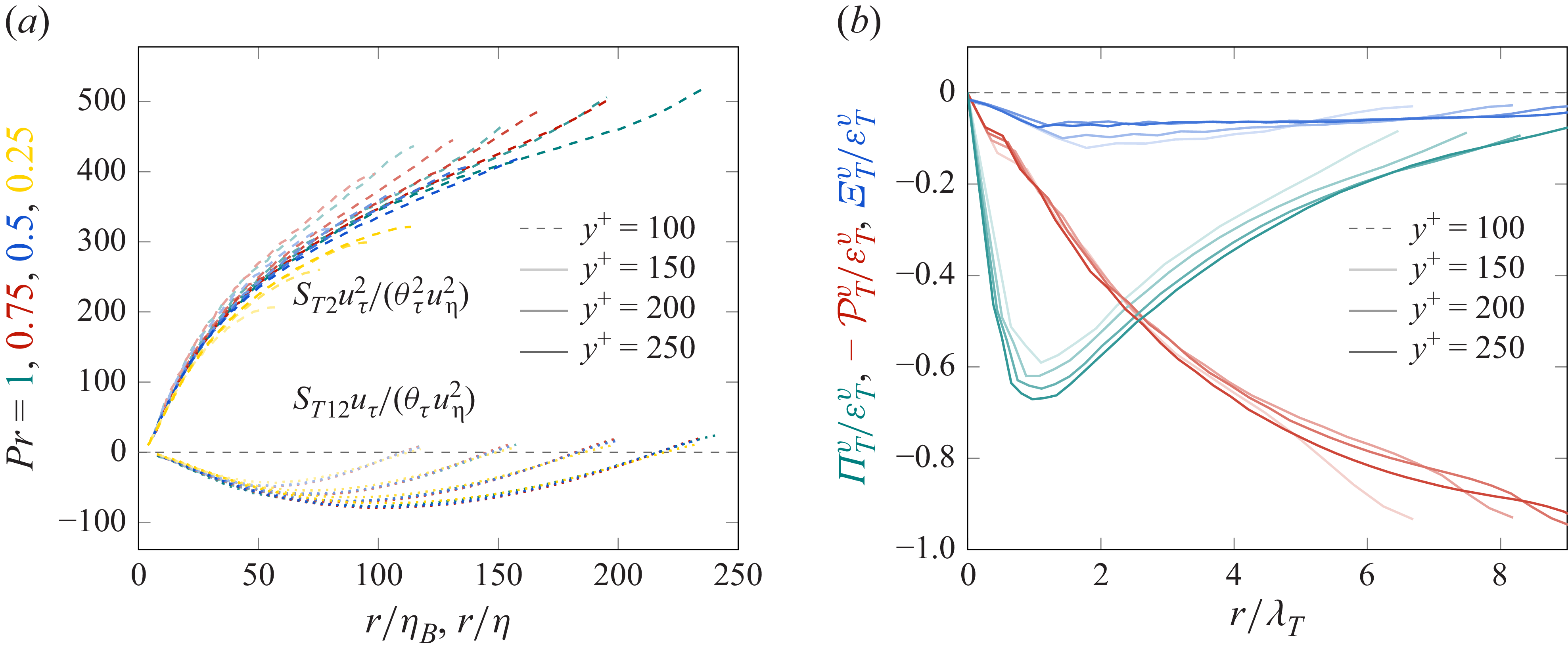
In this section, we use TCF DNS data to verify the theoretical conclusions in §§ 3.1 and 3.2. Figure 1(a) verifies the validity of the derived inner scalings
 $S_{T2} = \theta _\tau ^2 u_{\tau }^{-2} u_{\eta }^{2} F(r/\eta _{B})$
and
 $S_{T12} = \theta _\tau u_{\tau }^{-1} u_{\eta }^{2} G(r/\eta )$
by reporting how
 $S_{T2} u_\tau ^2 /(\theta _\tau ^2 u_\eta ^2)$
and
 $S_{T12} u_\tau /(\theta _\tau u_\eta ^2)$
evolve as functions of
 $r/\eta _B$
and
 $r/\eta$
, respectively. The collapse of the two sets of curves at small scales is not perfect, but is satisfactory if we consider that our DNS values of
 $\textit{Re}_{\tau }$
and
 $\textit{Re}_{\tau } Pr$
are not as large as might be required by our asymptotic analysis.
Figure 1(b) represents different terms in the balance (2.1) integrated over the volume of a sphere of radius
 $r/2$
, at different wall-normal locations. The results for the case
 $Pr=1$
are reported for conciseness, but similar behaviour is observed for our other
 $Pr$
values. Green lines represent inter-scale transfer rate and red lines represent production rate, both normalised by the volume integral of the two-point dissipation rate. In blue, we report the terms neglected in the budget (3.1) to confirm that they are small: it is worth noticing that their value is not zero, indicating that due to the limited value of
 $\textit{Re}_\tau$
these redistribution processes are low but still weakly active.
The qualitative behaviour of the different terms of the budget equations is similar for the velocity (Apostolidis et al. Reference Apostolidis, Laval and Vassilicos2023) and the passive scalar. The production rate increases as
 $r/\lambda _T$
increases above 1: at the smallest scales below
 $\lambda _T$
, the production rate is small, but it is present and non-negligible at all scales larger than
 $\lambda _T$
reaching, at the largest scales, the one-point log-layer equilibrium
 $\mathcal{P}_T^v\approx \varepsilon _T^v$
.
The inter-scale transfer rate is negative at all scales, indicating a cascade from large to small scales on average. As predicted in the previous sub-section, the minima of
 $\varPi _T^v/\varepsilon _T^v$
happen at similar values of
 $r/\lambda _T$
for all
 $y^+$
, and
 $(\varPi _T^v/\varepsilon _T^v)_{\textit{min}}$
decreases as
 $y^+$
and local
 $\textit{Re}_{\lambda }$
increase. The production-generated systematic departure from Kolmogorov two-point equilibrium is present throughout the inertial range, i.e. at all scales larger than
 $\lambda _T$
.
Scale
 $r_{\textit{min}}$
of
 $\varPi _T^v/\varepsilon _T^v$
minima as a function of wall distance
 $y^+$
(a–c) and values of
 $1 + \varPi _T^v/\varepsilon _T^v$
as a function of
 $\textit{Re}_\lambda$
(b–d). Top panels: Quantities not scaled with
 $Pr$
. Bottom panels: Quantities scaled with
 $Pr$
. The dashed line in the right panels is proportional to
 $\textit{Re}_\lambda ^{-2/3}$
.

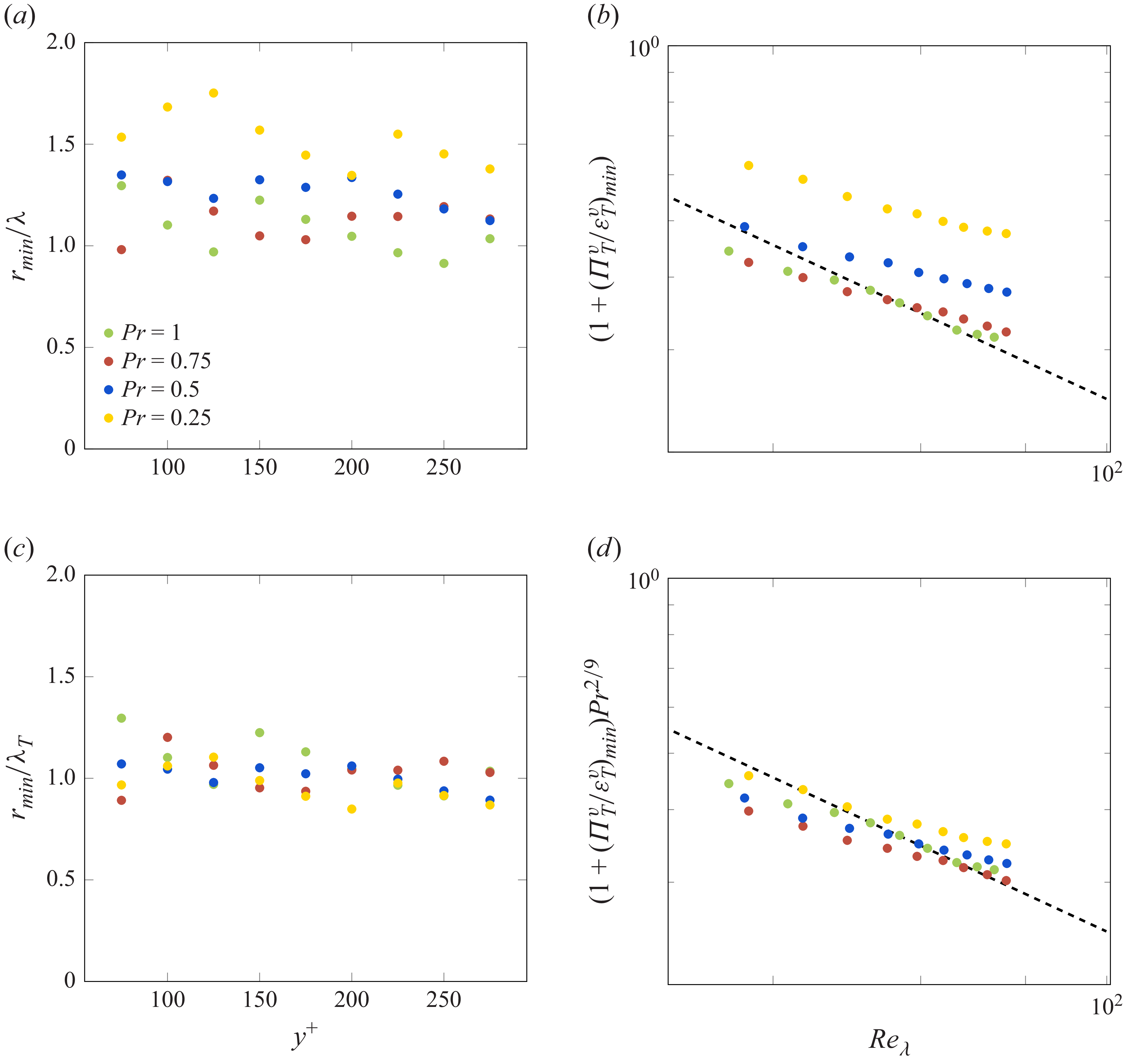
The theoretical relations (3.19)–(3.20) for the passive scalar stemming from our matched asymptotic expansion are quantitatively verified in figure 2 for different
 $Pr$
. The left panels show the length scale
 $r_{\textit{min}}$
of the minimum of the ratio between the inter-scale transfer and dissipation rates versus
 $y^+$
. In panel (a),
 $r_{\textit{min}}$
is normalised with
 $\lambda$
, and in panel (c) with
 $\lambda _T$
. For all cases,
 $r_{\textit{min}}$
collapses once scaled with
 $Pr^{-1/3}$
, i.e. as
 $r/\lambda _T$
. The minimum is at an almost constant value of
 $r/\lambda _T \sim 1$
for all
 $y^+$
in the intermediate layer and all our
 $Pr$
values in agreement with (3.19). The right panels of figure 2 show
 $1+(\varPi _T^v/\varepsilon _T^v)_{\textit{min}}$
versus
 $\textit{Re}_\lambda$
(which varies with
 $y^+$
). Considering the relatively low values of
 $\textit{Re}_{\lambda }$
, the data collapse quite well on the line
 $\textit{Re}_\lambda ^{-2/3}$
once multiplied by
 $Pr^{2/9}$
, as per our prediction (3.20). The turbulent Reynolds numbers
 $\textit{Re}_{\lambda }$
are not high, and their range is narrow in the intermediate layer at
 $\textit{Re}_{\tau }=1000$
. Due to the limited Reynolds number and the narrow dynamical range, deviations from the theoretical model are to be expected. Similar deviations were also pointed out by Apostolidis et al. (Reference Apostolidis, Laval and Vassilicos2023) at
 $\textit{Re}_\tau =1000$
, who also observed their reduction at
 $\textit{Re}_\tau =2000$
. The departure from this theoretical prediction increases as
 $Pr$
decreases. Indeed, the theoretical prediction is made for
 $\textit{Re}_\tau \gg 1$
and
 $\textit{Re}_{\tau } Pr \gg 1$
and the condition
 $\textit{Re}_{\tau } Pr \gg 1$
progressively weakens with decreasing
 $Pr$
for a given
 $\textit{Re}_{\tau }$
(as is the case in figure 2). The logarithmic region also becomes less well defined as
 $Pr$
decreases (Alcántara-Ávila et al. Reference Alcántara-Ávila, Hoyas and Pérez-Quiles2018). The best DNS agreement with the theoretical scaling (3.20) occurs for
 $Pr=1$
which is the case where
 $RePr$
is the highest in our DNS data. As
 $Pr$
decreases while keeping
 $\textit{Re}_{\tau }$
constant, the properties of the scalar intermediate layer which lead to our theoretical predictions deteriorate, namely, the assumed scaling of the turbulent scalar dissipation rate
 $\varepsilon _{T}^{v}$
and the presence of a well-developed approximate log layer for the passive scalar. Finally,
 $\textit{Re}_{\lambda }$
increases as
 $y^+$
increases and as
 $y^+$
increases we move towards the edge and out of the intermediate layer where the theoretical predictions are designed for.
3.4. Inter-scale transfer rate analysis
Decomposition of the inter-scale transfer rate into anti-aligned (blue lines) and aligned (red lines) contributions for
 $Pr=1$
. (a): Velocity; (b): Temperature.

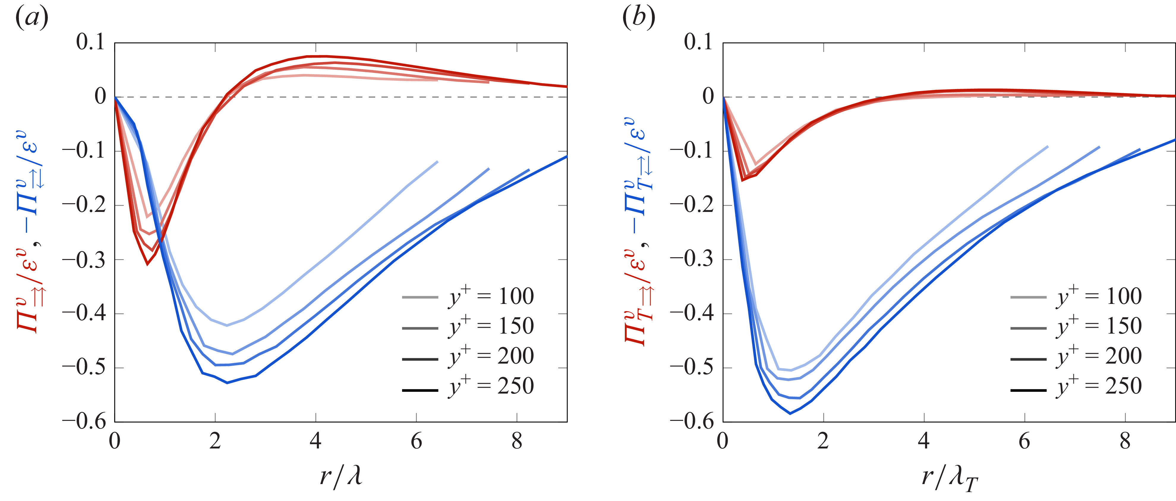
Given that the previous sub-section’s results for the passive scalar fluctuations are similar to those of Apostolidis et al. (Reference Apostolidis, Laval and Vassilicos2023) for the velocity fluctuations in the same flow, this section focuses on a more detailed comparison between inter-scale transfer of turbulent energy and turbulent scalar variance. In figure 3 we concentrate on our highest
 $\textit{Re}_{\tau } Pr$
value (i.e.
 $Pr=1$
) and plot inter-scale transfer rates decomposed into aligned and anti-aligned contributions for the velocity (a) and temperature (b). Aligned and anti-aligned contributions arise from the following decomposition introduced by Apostolidis et al. (Reference Apostolidis, Laval and Vassilicos2023) for the inter-scale turbulent energy transfer rate
 $\varPi ^v$
and explicitly given here for
 $\varPi _T^v$
:
 \begin{equation} \varPi _T^v=\varPi _{T\rightleftarrows }^v+\varPi _{T\rightrightarrows }^v = \frac {3}{4\pi }\int \text{d}\varOmega \! \left \langle { \frac {\delta \boldsymbol{u}'\boldsymbol{\cdot }\hat {\boldsymbol{r}}}{r} \delta \theta '\delta \theta '} \right \rangle \!_\rightrightarrows +\frac {3}{4\pi }\int \text{d}\varOmega \! \left \langle { \frac {\delta \boldsymbol{u}'\boldsymbol{\cdot }\hat {\boldsymbol{r}}}{r} \delta \theta '\delta \theta '} \right \rangle \!_{\rightleftarrows } ,\end{equation}
where the conditional average
 $ \! \left \langle {\ldots } \right \rangle \!_\rightrightarrows$
is taken over pairs of points where fluctuating velocities are aligned, i.e.
 $\boldsymbol{u}'(\boldsymbol{x}+\boldsymbol{r}/2)\boldsymbol{\cdot }\boldsymbol{u}'(\boldsymbol{x}-\boldsymbol{r}/2)\gt 0$
, and the conditional average
 $ \! \left \langle {\ldots } \right \rangle \!_{\rightleftarrows }$
is taken over pairs of points where fluctuating velocities are anti-aligned, i.e.
 $\boldsymbol{u}'(\boldsymbol{x}+\boldsymbol{r}/2)\boldsymbol{\cdot }\boldsymbol{u}'(\boldsymbol{x}-\boldsymbol{r}/2)\lt 0$
. Both
 $\varPi ^v$
and
 $\varPi _T^v$
involve the multiplication of the second-order structure functions (respectively of velocity and temperature) and the projected velocity difference
 $\delta \boldsymbol{u}' \boldsymbol{\cdot }\hat {\boldsymbol{r}}$
. The local sign of the velocity and temperature cascades is fully determined by
 $\delta \boldsymbol{u}' \boldsymbol{\cdot }\hat {\boldsymbol{r}}$
, with compressions (
 $\delta \boldsymbol{u}' \boldsymbol{\cdot }\hat {\boldsymbol{r}}\lt 0$
) causing forward cascades and stretchings (
 $\delta \boldsymbol{u}' \boldsymbol{\cdot }\hat {\boldsymbol{r}}\gt 0$
) causing inverse cascades. Clearly, the local sign of the cascade is not enough to compute its average value which stems from weighted averaging as per the above equation. Note that both aligned and anti-aligned components can involve both compressions and stretchings and therefore result in either a forward or inverse cascade component. Our results for the scalar fluctuations and those of Apostolidis et al. (Reference Apostolidis, Laval and Vassilicos2023) for the velocity fluctuations show that
 $\varPi _T^v$
and
 $\varPi ^v$
have similar evolutions with
 $r/\lambda _T$
and
 $r/\lambda$
, respectively, and that they are both negative at all the scales, meaning that local compressions dominate over local stretchings on average. In figure 3 we compare how aligned and anti-aligned pairs of velocity contribute to the cascade for the velocity and the cascade for the scalar. The anti-aligned components decrease and reach a minimum at a scale
 $r\gt r_{\textit{min}}$
, and then increase towards zero as expected since production balances dissipation at the largest scales. They dominate the inter-scale transfer rates at scales
 $r\gt r_{\textit{min}}$
and show similar evolutions with
 $r/\lambda$
-
 $r/\lambda _T$
for
 $\delta \boldsymbol{u}'\delta \boldsymbol{u}'$
and
 $\delta \theta '\delta \theta '$
. The aligned contributions to the inter-scale transfer rate also show similar evolutions with
 $r/\lambda$
-
 $r/\lambda _T$
for
 $\delta \boldsymbol{u}'\delta \boldsymbol{u}'$
and
 $\delta \theta '\delta \theta '$
, reaching a minimum at a scale
 $r\lt r_{\textit{min}}$
for both the scalar and the velocity cases. Despite these similar evolutions, the aligned contributions are clearly different as their magnitude is significantly lower for the temperature than for the velocity fields. Furthermore, the peak value of
 $\varPi _{\rightleftarrows }^v/\varepsilon ^v$
appears to coincide in
 $r$
with the zero value of
 $\varPi _{\rightrightarrows }^v/\varepsilon ^v$
(where
 $\varepsilon ^v$
is the sphere-averaged turbulence dissipation rate). If this coincidence (figure 3) persists as
 $\textit{Re}_{\tau }\to \infty$
then the intermediate asymptotic theory of Apostolidis et al. (Reference Apostolidis, Laval and Vassilicos2023) would imply that
 $\varPi _{\rightleftarrows }^v/\varepsilon ^v$
tends to
 $-1$
in that limit. However, the peak value of
 $\varPi _{T\rightleftarrows }^v/\varepsilon _{T}^v$
does not coincide in
 $r$
with the zero value of
 $\varPi _{T\rightrightarrows }^v/\varepsilon _{T}^v$
as clearly seen in 3. If this lack of coincidence persists as
 $\textit{Re}_{\tau }\to \infty$
then (3.20) would imply that
 $\varPi _{T\rightleftarrows }^v/\varepsilon _{T}^v$
does not tend to
 $-1$
in that limit. Even though the overall physical process determining the direction of the cascade is the same for velocity and temperature (compressions and stretchings via
 $\delta \boldsymbol{u}' \boldsymbol{\cdot }\boldsymbol{n}$
), there are significant differences arising from whether compressions and stretchings result from aligned or anti-aligned fluctuating velocities. The explanation of these differences will require a dedicated future study which may need to consider the underlying flow structure of the turbulence, for example, in terms of ejections and sweeps.
4. Conclusions
We performed a scale-by-scale analysis of passive scalar fluctuations in the intermediate layer of a fully developed TCF to assess the presence or absence of a Kolmogorov-like equilibrium. The TCF analysis of Apostolidis et al. (Reference Apostolidis, Laval and Vassilicos2023) has had to be non-trivially extended to account for a passive scalar with Prandtl number
 $Pr \leqslant 1$
in the limit
 $\textit{Re}_{\tau } Pr \gg 1$
. It transpired from our hypothesis of homogeneous physics in non-homogeneous turbulence combined with the Navier–Stokes equation that the scalar fluctuations’ inner length scale is the Reference BatchelorBatchelor length even though the turbulence in the channel flow’s intermediate layer is not homogeneous down to very small scales. Indeed, the Batchelor length was originally introduced by Batchelor (Reference Batchelor1959) for homogeneous turbulence, yet two-point turbulent scalar production, and therefore non-homogeneity, in the channel flow’s intermediate layer is significant down to length scales as small as
 $\lambda _{T} = \lambda Pr^{-1/3}$
. It also follows from our analysis that the scalar field’s average inter-scale transfer rate is negative (forward cascade on average) and maximal at a specific length scale
 $r_{\textit{min}}\sim \lambda _{T}$
. The tendency towards a Kolmogorov equilibrium between scalar inter-scale transfer rate and scalar dissipation rate is achieved asymptotically (
 $\textit{Re}_{\tau } \to \infty$
) at that length scale only, and systematic departures from this equilibrium are present and increase with length scale throughout the inertial range because of the presence of two-point scalar turbulence production. These theoretical arguments have been verified with DNS of turbulent velocity and scalar fields in channel flow at different Prandtl numbers
 $Pr=1$
,
 $0.75$
,
 $0.5$
and
 $0.25$
. Good agreement has been found between the hypotheses and the predictions on the one hand, and the DNS data on the other. Even though the aforementioned results and respective ones in Apostolidis et al. (Reference Apostolidis, Laval and Vassilicos2023) demonstrate a close analogy between the inter-scale transfer properties of turbulent velocity and scalar fields in the intermediate layer of TCF, there are some significant differences between them. Whilst the inter-scale transfer rates
 $\varPi ^v$
(for the fluctuating velocity) and
 $\varPi _T^v$
(for the fluctuating scalar) have similar evolutions with length scale
 $r$
, the contributions from aligned and anti-aligned pairs of fluctuating velocities differ for
 $\varPi ^v$
and
 $\varPi _T^v$
.
Acknowledgements
This collaboration started when G.K. was visiting the LMFL as Visiting Professor at the University of Lille from 27 October to 9 November 2024. J.C.V. acknowledges funding by the European Union (ERC Advanced Grant NoStaHo, project number 101054117). Views and opinions expressed are, however, those of the author(s) only and do not necessarily reflect those of the European Union or the European Research Council. Neither the European Union nor the granting authority can be held responsible for them. This project was provided with computing HPC and storage resources by GENCI at CINES thanks to the grant 2025-A0182A01741 on the supercomputer Adastra’s GENOA partition.
Declaration of interests
The authors report no conflicts of interest.