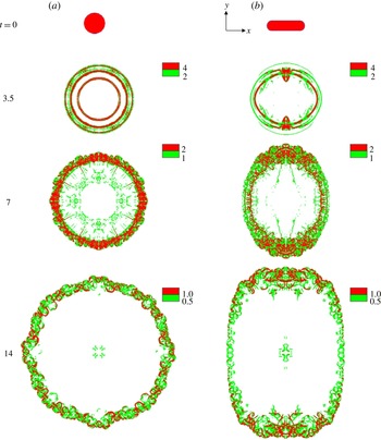
1. Introduction
Gravity or density currents are horizontal flows generated from a difference in density between two fluids. They encompass a wide variety of environmental and industrial flows that are often catastrophic in nature. Some of the many examples include avalanches (Allen Reference Allen1982), oil spills (Kubat, Holte & Matwin Reference Kubat, Holte and Matwin1998), turbidity currents (Lowe Reference Lowe1982), sand storms (Bagnold Reference Bagnold1941) and pyroclastic eruptions (Francis Reference Francis and Francis1993). The density difference can be a result of variations of temperature (a cold breeze of air intruding into a hot ambient), salinity (fresh water from a river draining into the salty dense ocean), or inhomogeneous distribution of particles in suspension (a turbid mixture of fluid–particles advancing into a clear ambient). Depending on the density ratio of the two fluids, gravity currents are categorized as heavy bottom-flowing currents, when the intruding fluid is denser than its ambient, and light top-flowing currents, when the intruding fluid is lighter than its surrounding ambient. Furthermore, gravity currents can be simplified as Boussinesq (heavy or light) currents when the density difference is much smaller than the current and the ambient densities.
Gravity currents, when propagating horizontally into their ambient, usually undergo four main stages (Huppert & Simpson Reference Huppert and Simpson1980). Initially, when the current is released, it accelerates from rest until it reaches a maximum velocity. During this highly transitional phase, termed the acceleration phase, the current undergoes rapid change in its velocity (zero to maximum) and the structure of the release also changes from mostly vertical to horizontal. This phase is often overlooked for three main reasons: (1) it is complex and transitional in nature, (2) it is relatively short-lived in duration, and (3) it is presumed to have little effect on the long-term dynamics of the current. Following the acceleration phase, the current reaches a steady-state phase, referred to as the slumping phase. During this phase, a planar (circular) current advances with a constant (nearly constant) velocity and height (Gladstone, Phillips & Sparks Reference Gladstone, Phillips and Sparks1998). At the end of the slumping phase, the current typically transitions to the inertial self-similar phase, where the buoyancy driving force is balanced by the current’s inertia. During this phase, the current starts to decelerate as a consequence of its diminishing front height. Finally, as the current’s thickness continues to decrease, viscous and/or capillary forces become dominant, and the current evolves into the self-similar viscous/capillary phase.
Fixed-volume releases have been extensively investigated over the past several decades (see e.g. Simpson Reference Simpson1982) generally through one of two canonical configurations, namely planar (Britter & Simpson Reference Britter and Simpson1978; Rottman & Simpson Reference Rottman and Simpson1983) or axisymmetric (Didden & Maxworthy Reference Didden and Maxworthy1982; Huq Reference Huq1996) geometry. In the planar release case, a flat rectangular gate initially separates a rectangular reservoir of fluid from an ambient of different, usually lower, density. Similarly, at the start of the axisymmetric three-dimensional release, the release is confined inside a hollow circular cylinder at the centre of a large tank containing the ambient fluid (Huppert Reference Huppert1982; Cantero, Balachandar & Garcia Reference Cantero, Balachandar and Garcia2007b
), or in an expanding reservoir of relatively small angle of expansion, typically
 $10^{\circ }$
–
 $15^{\circ }$
(Huppert & Simpson Reference Huppert and Simpson1980).
By considering an idealized inviscid current and neglecting mixing at the interface, Benjamin (Reference Benjamin1968) derived his well-known Froude-number expression
 $u_{N}=\mathit{Fr}\sqrt{g^{\prime }h_{N}}$
relating the front velocity
 $u_{N}$
of a slumping steady-state gravity current to the front height
 $h_{N}$
(
 $g^{\prime }$
is the reduced gravity). He showed that the Froude number
 $\mathit{Fr}$
is solely dependent on the relative depth of the ‘head’ of the current with respect to the ambient. His idealized energy balance analysis restricted the maximum attainable front height in a confined geometry to half the total depth of the ambient fluid. However, as Benjamin recognized, the turbulent nature of gravity currents coupled with mixing along the interface of the current necessitates the use of semi-empirical analysis to more accurately quantify the evolution of the front of such complex flows.
Huppert & Simpson (Reference Huppert and Simpson1980) later conducted a large number of planar and axisymmetric fixed-volume experiments to examine the slumping phase of gravity currents. They varied several parameters, including the initial depth ratio (ratio of the height of the current to that of the ambient), the vertical aspect ratio (initial ratio of the height to the length or radius of the current), the initial volume of release and the density ratio. They proposed that, during the slumping phase, a planar (respectively axisymmetric) current’s evolution could be modelled as a series of two-dimensional rectangles (respectively concentric circular disks) with negligible entrainment (this is the basis for the box model analysis discussed later in the paper). The experiments further confirmed that the slumping motion of the current is controlled by the head, and the authors proposed a correlation for the Froude-number expression from their experimental data. Their semi-empirical Froude-number expression, again, solely depends on the fractional depth of the current (see e.g. (3.9)).
Studies of gravity currents beyond the classical planar or axisymmetric framework have been rare to our knowledge, despite the fact that the majority of gravity currents in real situations originate from an arbitrary, usually non-axisymmetric, configuration. The underlying assumption is that the initial details of the release are soon forgotten after the release.
Recently, Zgheib, Bonometti & Balacandar (Reference Zgheib, Bonometti and Balacandar2014) explored the slumping phase (short-term) and inertial self-similar phase (longer-term) behaviours of non-axisymmetric fixed-volume gravity currents. They demonstrated, through experiments and simulations, that gravity currents initiating from non-axisymmetric cross-sectional geometries do not become axisymmetric, nor do they retain their initial shape during the slumping and inertial phases of the current. In particular, the local speed of propagation of a material front, generated by the release of a patch of arbitrary shape, can vary significantly, thus leading to local ‘fast fronts’ and ‘slow fronts’ during all the observed phases of spreading. They explained the dynamics of non-circular gravity currents by observing that, during the acceleration and early part of the slumping phases, the initial release appears to partition itself into local volumes along the front. The subsequent outward propagation of the front is dictated by these local volumes (in particular the local height of the front) along the direction locally normal to the front. Using this key observation, they developed a simple locally dependent box model, referred to as the extended box model (EBM) that is based on a partitioning of the initial release and local front velocity, and showed that the EBM could predict with a reasonable degree of accuracy the dynamics of non-circular gravity currents, both temporally and spatially.
The present paper aims at answering some remaining open questions regarding the dynamics of non-circular gravity currents. The shape of the propagating front of a planar or an axisymmetric current, by definition, remains self-similar. Furthermore, in the different regimes of propagation, their speed follows self-similar power laws in time. In the case of a non-axisymmetric initial release, the shape of the propagating front substantially differs from the initial release and remains non-axisymmetric. Some natural questions arise. Does the propagating front evolve towards a self-similar non-axisymmetric shape? If so, what is the relation between this self-similar shape of the spreading current and the shape of the initial release? The applicability of the EBM is validated against two sets of direct numerical simulations and subsequently the EBM is used to study the self-similar evolution of a wide range of initial releases of different aspect ratio.
The non-axisymmetric self-similar shape of the propagating front requires that the front velocity be self-similar as well. We also explore the local Froude-number variation of the current along the circumference of the non-axisymmetric current and compare the simulation results with those from existing front Froude-number relations. In addition, we use the results of the fully resolved direct numerical simulations to (i) describe the local flow structure of non-axisymmetric gravity currents and (ii) evaluate the validity of the assumptions used in the EBM.
In this work we also examine the robustness and the range of validity of the observed dependence of non-axisymmetric spreading on the shape of the initial release. Zgheib et al. (Reference Zgheib, Bonometti and Balacandar2014) reported the results for only Boussinesq saline currents spreading along the bottom boundary. Here we consider non-Boussinesq currents, lighter currents spreading on the top surface, and demonstrate that the dependence of non-axisymmetric spreading on the shape of the initial release persists in all these cases. Only in the case of low-Reynolds-number
 $(\mathit{Re}\sim O(100))$
non-axisymmetric releases do viscous effects dominate and the current is observed to evolve to a circular shape.
This paper is arranged as follows. The experimental and numerical set-ups are presented in § 2. The question of the self-similarity of the shape of non-axisymmetric high-Re currents and the relevance of the models of front Froude function are addressed in § 3. In § 4, we discuss the assumptions used in the EBM and use the EBM to propose a scaling law for the prediction of the self-similar shape of non-axisymmetric gravity currents. The effect of the initial vertical and horizontal aspect ratios is examined in § 5. In §§ 6 and 7, we discuss the vortical structures and present some qualitative and quantitative investigations of other types of currents, respectively. Finally, concluding remarks of the present findings are given in § 8.
2. Experimental and numerical procedures
2.1. Experimental set-up
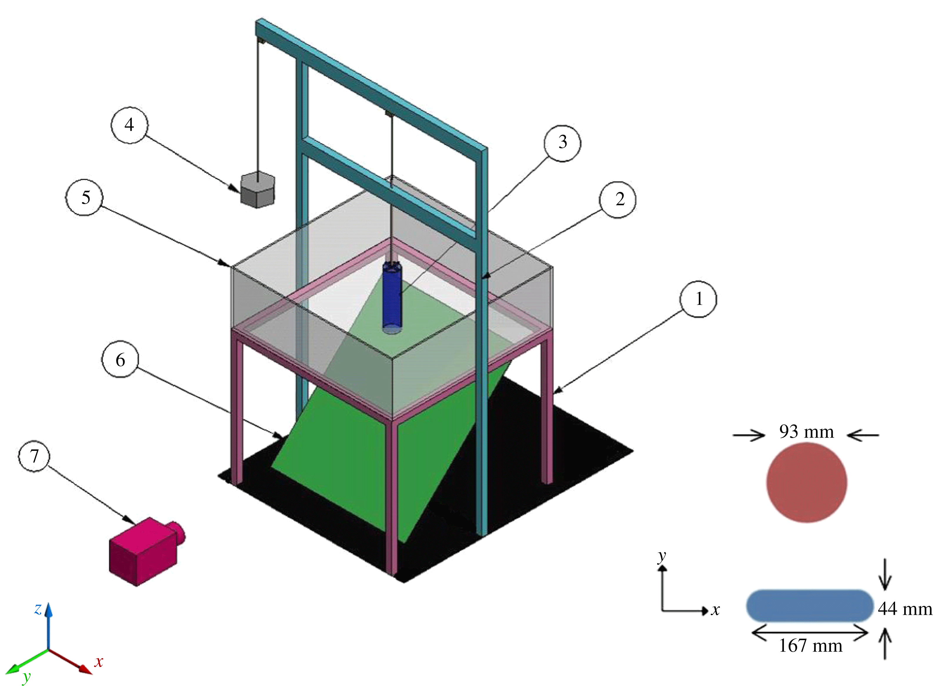
The experimental set-up is shown in figure 1. The experiments are carried out in a glass square tank (
 $120~\text{cm}\times 120~\text{cm}\times 40~\text{cm}$
) at the centre of which we place a hollow cylinder of equivalent radius
 $R_{0}$
, filled up to a height
 $h_{0}$
with a fluid of different density than the ambient fluid of height
 $H$
. Two different cross-sectional shapes are considered, namely a circular section (CS) for verification and comparison with previous results and a rounded rectangular section (RR), i.e. a rectangle where the two shorter edges are replaced by semicircles. The initial horizontal aspect ratio
 ${\it\chi}_{0}$
of the rounded rectangular cylinder, here defined as the ratio of the longest to the shortest side, is
 ${\it\chi}_{0}=3.8$
. Fluorescent dye is added to the fluid inside the cylinder. Black light tubes mounted on two sides of the tank illuminate the fluorescent dye inside a dark room, allowing the current to be solely visible.
Experimental set-up:
 $\unicode[STIX]{x2460}$
tank support,
 $\unicode[STIX]{x2461}$
pulley support,
 $\unicode[STIX]{x2462}$
hollow cylinder,
 $\unicode[STIX]{x2463}$
pulley weight,
 $\unicode[STIX]{x2464}$
tank,
 $\unicode[STIX]{x2465}$
mirror,
 $\unicode[STIX]{x2466}$
camera. The experiments are carried out with two different cross-sectional geometries, namely a circular section (CS) and a rounded rectangle (RR). Both geometries have roughly the same cross-sectional area, leading to an equivalent radius
 $R_{0}$
of 4.6 and 4.7 cm for the CS and RR geometry, respectively,
 $R_{0}$
being calculated from the surface area
 $A$
as
 $R_{0}=\sqrt{A/{\rm\pi}}$
. An inclined mirror is placed underneath the tank, so that the current’s evolution is recorded from both the side and below. The square tank dimensions are
 $120~\text{cm}\times 120~\text{cm}\times 40~\text{cm}$
, corresponding to approximately
 $26R_{0}\times 26R_{0}\times 9R_{0}$
. Gravity is pointing towards the
 $z$
direction.

Unless stated otherwise, the ambient fluid is tap water of density
 ${\it\rho}_{a}=1000~\text{kg}~\text{m}^{-3}$
while the current consists of salty water of density
 ${\it\rho}_{c}=1100~\text{kg}~\text{m}^{-3}$
. The depth ratio
 $h_{0}/H$
(ratio of lock height to that of the ambient) for all the experiments was held at unity. The initial vertical aspect ratio
 ${\it\lambda}=h_{0}/R_{0}$
(height/radius) was varied between 0.25 and 7. The radius
 $R_{0}$
for the non-axisymmetric cross-sections is calculated from the surface area
 $A$
via
 $R_{0}=\sqrt{A/{\rm\pi}}\approx 4.6$
cm. The two geometries were chosen to have roughly the same cross-sectional area, so that, for a fixed initial height, the volume of release is constant whatever the initial cross-sectional shape. The tank and the cylinder are simultaneously filled. When the desired vertical aspect ratio is reached, the water in the tank is given sufficient time to reach a stagnant state. The hollow cylinder is then raised rapidly via a pulley system connected to a weight.
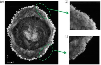
The front location and the current’s height are measured using a mirror placed beneath the tank, which allows for a plan bottom view of the front evolution (e.g. figure 2), while the side view of the current provides information about the evolution of the current height (e.g. figure 5). The pixel resolution was approximately
 $R_{0}/82$
(0.5 mm) and
 $h_{0}/44$
(2 mm) for a
 ${\it\lambda}=2$
release in the horizontal and vertical directions, respectively. The front location is obtained from the plan view images using the MATLAB® Graphics in-built function Imread®, where each pixel is assigned a value in the intensity range
 $[0,255]$
. All values between 1 and 254 can be considered as different shades of grey (0 corresponding to the black colour). The front is easily determined since there is a significant jump (within a few pixels) in the intensity levels at the current–ambient interface. Note that the location of the front was found to be insensitive to the chosen cut-off value. As can be seen from the example in figure 2, the location of the front is well extracted.
Example of front location detection from experiments. A plan view of the current (Exp 2 at
 $t=5.9$
) is shown in (a) along with the white star symbols corresponding to the extracted front location. The close-up views in (b,c) show good agreement between the extracted and the actual front location. (See supplementary movie available at http://dx.doi.org/10.1017/jfm.2015.580.)

The local front location is then computed as follows. The local radial location of the front
 $\overline{r_{N}}({\it\theta}t)$
, along the azimuthal
 ${\it\theta}$
direction is first calculated by averaging along a sector of angle
 $2{\it\alpha}_{0}={\rm\pi}/36$
around the front location as
 $$\begin{eqnarray}\overline{r_{N}}({\it\theta},t)=\frac{1}{2{\it\alpha}_{0}}\int _{{\it\theta}-{\it\alpha}_{0}}^{{\it\theta}+{\it\alpha}_{0}}r_{N}({\it\theta},t)\,\text{d}{\it\theta},\end{eqnarray}$$
where the
 ${\it\theta}$
coordinate’s origin is taken along the
 $x$
direction and
 $r_{N}({\it\theta}t)$
is the radial distance at time
 $t$
between the initial centre of mass of the current and a point at the front of the current. We further use the symmetry of the flow, when applicable, by taking the average value of
 $\overline{r_{N}}({\it\theta},t)$
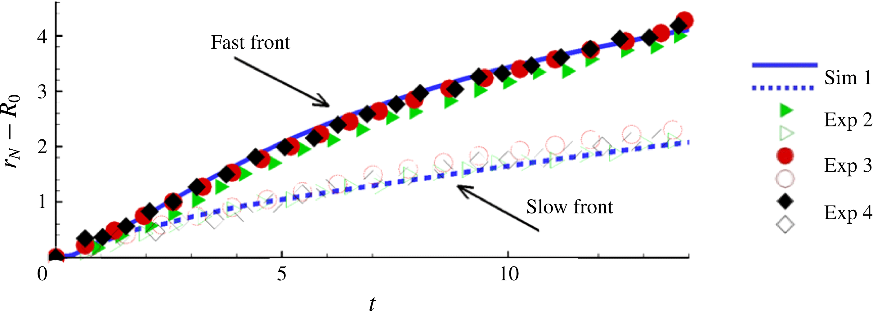
along the symmetry directions. For instance, the ‘fast’ front position in figure 3 is computed as
 $\overline{r_{F}}(t)=[\overline{r_{N}}({\it\theta}=0,t)+\overline{r_{N}}({\it\theta}={\rm\pi},t)]/2$
and similarly for the ‘slow’ front position, i.e.
 $\overline{r_{S}}(t)=[\overline{r_{N}}({\it\theta}={\rm\pi}/2,t)+\overline{r_{N}}({\it\theta}=3{\rm\pi}/2,t)]/2$
. For all the non-axisymmetric cases, we selected the fastest and slowest sections of the front, all other directions hence having velocity magnitudes bounded between these values.
Time evolution of the front position of the ‘slow’ and ‘fast’ fronts of RR currents for various initial orientations of the rounded rectangular cylinder relative to the tank walls. The angle between the initial longest side of the RR cylinder and the tank wall is
 $0^{\circ }$
(Exp 2),
 $45^{\circ }$
(Exp 3) and
 $90^{\circ }$
(Exp 4), respectively. The front location is averaged over a small sector of width
 $2{\it\alpha}={\rm\pi}/36$
. Note that the tank walls are located at a minimum distance of
 $13R_{0}$
from the centre of mass of the current, which corresponds to
 $r_{N}-R_{0}=6$
here (recall that the front position is scaled by
 $h_{0}$
and that
 ${\it\lambda}=h_{0}/R_{0}=2$
here). For comparison, the results obtained with Sim 1, for which the ‘outer walls’ are at a minimum distance of
 $16R_{0}$
, is also plotted.

2.2. Preliminary verifications
As a preliminary verification, we performed two sets of experiments, in order to check that the outer vertical walls of the tank did not affect the dynamics of the non-circular gravity currents. In the first set of experiments, we consider three rounded rectangular releases under nominally identical conditions except that the initial orientation of the RR cylinder relative to the tank walls is varied; in particular, the angle between the initial longest side of the RR cylinder and the tank wall is
 $0^{\circ }$
,
 $45^{\circ }$
and
 $90^{\circ }$
in the experiments denoted as Exp 2, 3 and 4 in table 1, respectively. The temporal evolution of the slow and fast fronts is displayed in figure 3. The dynamics of the fronts is observed to be similar in all cases. The slight difference between the three realizations is indicative of experimental measurement uncertainty, which is much smaller than the observed difference between the fast and slow fronts.
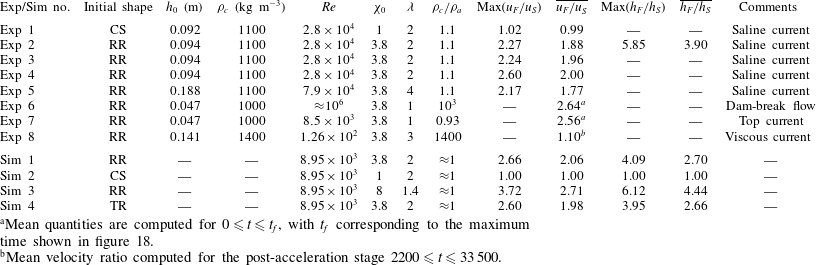
Velocity ratio
 $u_{F}/u_{S}$
and height ratio
 $h_{F}/h_{S}$
between the fastest and slowest points of some gravity currents of initially arbitrary shape. The mean quantities are computed for
 $0\leqslant t\leqslant 22$
(
 ${\it\lambda}=1.4$
),
 $0\leqslant t\leqslant 12.6$
(
 ${\it\lambda}=2$
) and
 $0\leqslant t\leqslant 6.5$
(
 ${\it\lambda}=4$
). CS, RR and TR refer to the circle, rounded rectangle and true rectangle, respectively (see figure 1). The initial vertical aspect ratio is
 ${\it\lambda}=h_{0}/R_{0}$
. (See supplementary movies.)

a
Mean quantities are computed for
 $0\leqslant t\leqslant t_{f}$
, with
 $t_{f}$
corresponding to the maximum time shown in figure 18.
b
Mean velocity ratio computed for the post-acceleration stage
 $2200\leqslant t\leqslant 33\,500$
.
The second set of experiments consists of placing two vertical panels, each at an opposite end of the tank and having the same width and height as the tank, at a distance of 10 cm (that is, roughly
 $2R_{0}$
) from the tank walls normal to the
 $x$
axis. In that case, the size of the tank is shorter in one direction by approximately
 $4R_{0}$
. We repeated the previous experiments of rounded rectangular releases in this smaller tank and compared the temporal evolution of the front position and velocity. It was found that the dynamics of the current were not affected by the presence of the wall as long as the current’s front was at a distance larger than
 $2R_{0}$
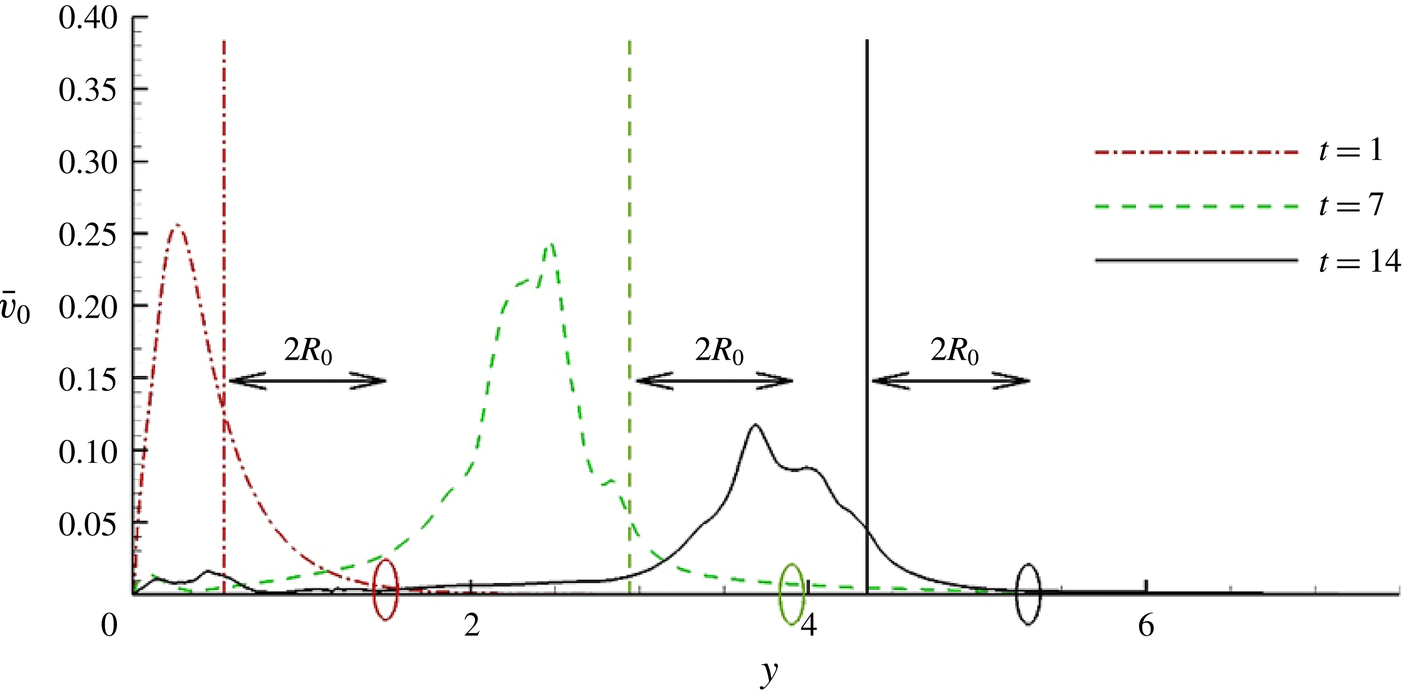
from the lateral walls (not shown). The above tests allow us to conclude that the dynamics of the non-circular gravity currents shown in the present experiments is not influenced by the presence, shape or orientation of the walls of the tank. This point will be further strengthened in § 7.5 by showing that the velocity of the ambient fluid beyond the front is much smaller than that of the current.
As a final verification, we use simple estimates to show that both the slumping and the inertial self-similar regimes of propagation are covered in the present experiments and simulations. By matching the (nearly) constant velocity during the slumping phase with the inertial phase scaling of a circular current, the transition time from the slumping to the inertial phase can be estimated as (Cantero et al. Reference Cantero, Lee, Balachandar and Garcia2007a )
 $$\begin{eqnarray}t_{SI}=\left(\frac{{\rm\pi}^{1/4}}{2}{\it\xi}_{c}\right)^{2}\frac{r_{0}h_{0}^{1/2}}{F_{c,sl}^{2}}.\end{eqnarray}$$
Hoult (Reference Hoult1972) and Huppert & Simpson (Reference Huppert and Simpson1980) have proposed the values
 ${\it\xi}_{c}=1.3$
and
 ${\it\xi}_{c}=1.16$
, respectively. The constant
 $F_{c,sl}\approx 0.3$
represents the mean front velocity during the slumping phase. For our axisymmetric release (Exp 1 and Sim 2), the transition time computed from (2.2) is
 $t_{SI}\approx 4.2$
(respectively 3.3), for
 ${\it\xi}_{c}=1.3$
(respectively 1.16). These values are well below the characteristic duration of the experiments and simulations, which is approximately 14. As will be confirmed later, the gravity currents presented here undergo the acceleration phase, the slumping phase and eventually the inertial self-similar phase.
2.3. Numerical procedure
In this paper, all the variables are dimensionless, choosing
 $h_{0}$
as length scale,
 $U=\sqrt{g^{\prime }h_{0}}$
as velocity scale,
 $h_{0}/U$
as time scale and
 ${\it\rho}_{a}$
as density scale (
 $g^{\prime }$
is the reduced gravity defined as
 $g^{\prime }=g({\it\rho}_{c}-{\it\rho}_{a})/{\it\rho}_{a}$
). We define
 $x$
(
 $y$
) as the direction of the major (minor) axis when applicable, and
 $z$
as the direction parallel to gravity.
The physical configuration of the simulations is identical to the experimental set-up. We solve the concentration equation along with the incompressible Navier–Stokes equations. The system reads in dimensionless form
 $$\begin{eqnarray}\displaystyle & \displaystyle \boldsymbol{{\rm\nabla}}\boldsymbol{\cdot }\boldsymbol{u}=0, & \displaystyle\end{eqnarray}$$
 $$\begin{eqnarray}\displaystyle & \displaystyle \frac{\text{D}\boldsymbol{u}}{\text{d}t}={\it\rho}\boldsymbol{e}^{g}-\boldsymbol{{\rm\nabla}}p+\frac{1}{\mathit{Re}}{\rm\nabla}^{2}u, & \displaystyle\end{eqnarray}$$
 $$\begin{eqnarray}\displaystyle & \displaystyle \frac{\partial {\it\rho}}{\partial t}+\boldsymbol{{\rm\nabla}}\boldsymbol{\cdot }({\it\rho}u)=\frac{1}{\mathit{Sc}\,\mathit{Re}}{\rm\nabla}^{2}{\it\rho}, & \displaystyle\end{eqnarray}$$
 $\boldsymbol{u}$
,
 $p$
and
 ${\it\rho}$
are the local velocity, total pressure and density in the flow, respectively, and
 $\boldsymbol{e}^{g}$
is a unit vector pointing in the direction of gravity. Two dimensionless parameters have been introduced in (2.4) and (2.5), namely the Reynolds number and the Schmidt number defined as
 $$\begin{eqnarray}\mathit{Re}=Uh_{0}/{\it\nu},\quad \mathit{Sc}={\it\nu}/{\it\kappa}.\end{eqnarray}$$
Here
 ${\it\kappa}$
is the molecular diffusivity and
 ${\it\nu}$
is the kinematic viscosity of the fluid. Equations (2.3)–(2.5) are solved inside a rectangular box of size
 $15\times 15\times 1$
with a spectral code (Cantero et al.
Reference Cantero, Lee, Balachandar and Garcia2007a
,Reference Cantero, Balachandar and Garcia
b
). Note that the experimental tank size was approximately
 $12\times 12$
in the
 $x$
–
 $y$
plane for
 ${\it\lambda}=2$
. No-slip and free-slip boundary conditions are imposed for the velocity at the bottom and top walls, respectively, while periodic boundary conditions are imposed at the sidewalls. Zero normal gradient is imposed for the density field at the bottom and top walls. Fourier expansions are used along the two horizontal periodic directions, and a Chebyshev expansion with Gauss–Lobatto quadrature points (Canuto et al.
Reference Canuto, Hussaini, Quarteroni and Zang1988) is used along the vertical non-periodic direction. The reader is referred to Cortese & Balachandar (Reference Cortese and Balachandar1995) and Cantero et al. (Reference Cantero, Balachandar and Garcia2007b
) for a detailed description of the numerical approach and for results obtained with the same code in axisymmetric configurations, respectively.
In the present work, we simulate the collapse of a non-axisymmetric patch of heavy fluid at
 $\mathit{Re}=8950$
with a grid resolution of
 $880\times 880\times 179$
corresponding to approximately 140 million grid points. The numerical resolution was selected to have between four and six decades of decay in the energy spectrum for all the variables, and the time step was selected to produce a Courant number smaller than 0.5. In the simulations, the Schmidt number is set to unity. Note that this value is smaller than that of a saline gravity current, for which
 $\mathit{Sc}\approx 700$
, but it has been shown that the dynamics of gravity currents is independent of the Schmidt number as long as the Reynolds number is large, which is the case here (Bonometti & Balachandar Reference Bonometti and Balachandar2008).
3. High-Reynolds-number Boussinesq density currents
In this section, we present results from experiments and fully resolved simulations of density currents of non-axisymmetric initial shape, the parameters of which are summarized in table 1. In particular, a detailed description of the local flow structure in this type of flow as compared to a circular release is given.
3.1. Self-similarity of the front shape in non-axisymmetric releases
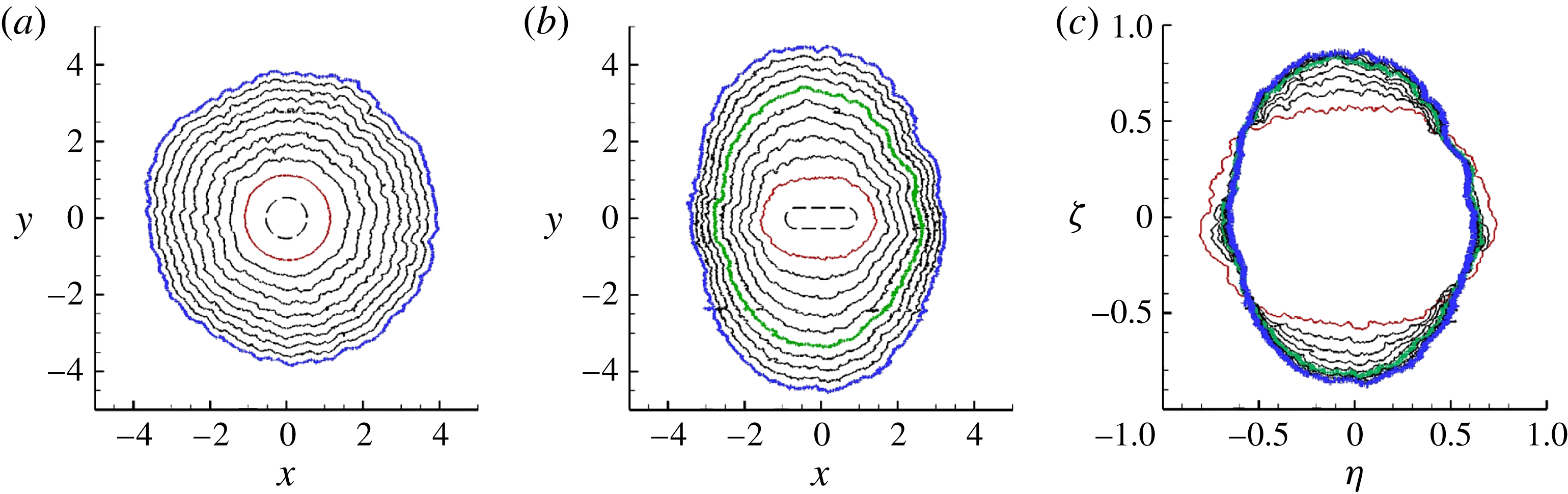
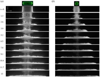
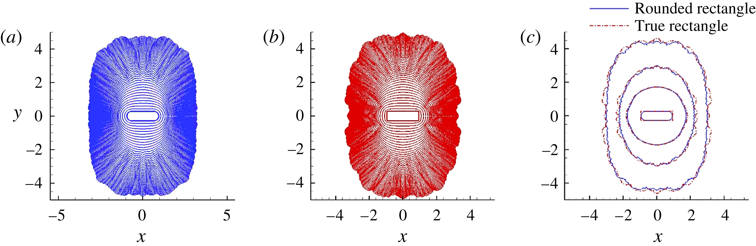
The temporal evolution of the spreading of gravity currents with two different initial cross-sectional shapes is presented in figure 4(a,b). The figure shows a plan view of a composite image of the front evolution for each experiment at various instants in time. The circular release is shown for comparison in panel (a). While the case of the circular release shows small undulations at the front due to the lobe and cleft instability (Simpson Reference Simpson1972; Härtel, Fredrik & Mattias Reference Härtel, Fredrik and Mattias2000), the current retains its overall symmetry as it propagates outwards. Conversely, for the RR current, as shown in Zgheib et al. (Reference Zgheib, Bonometti and Balacandar2014), the long-time circumferential shape is approximately an ellipse, but with switched major and minor axes as compared to the initial shape. Lobes and clefts are observed at the front even in this non-axisymmetric release. Note that the characteristic sizes of these lobes and clefts are an order of magnitude smaller than the length scale of the larger-scale flow pattern.
Evolution of the front contours for (a) a circular (Exp 1) and (b) a rounded rectangular release (Exp 2). Panel (c) is similar to panel (b) using the self-similar variables
 ${\it\eta}=xt^{-1/2}$
and
 ${\it\zeta}=yt^{-1/2}$
, respectively. Note that here the variables are dimensionless, so that in dimensional form the self-similar variables would become
 ${\it\eta}=(g^{\prime }h_{0}^{3})^{-1/4}\tilde{x}\tilde{t}^{-1/2}$
and
 ${\it\zeta}=(g^{\prime }h_{0}^{3})^{-1/4}{\tilde{y}}\tilde{t}^{-1/2}$
, respectively (where the tilde denotes a dimensional variable). The contours are plotted from
 $t_{0}=2.1$
(red curve) to
 $t_{f}=13.8$
(blue curve) in steps of
 ${\rm\Delta}t=1.3$
. Plotted in green is the curve corresponding to a time of
 $t=8.6$
for which the shape becomes roughly self-similar. It is noteworthy that, at the time
 $t_{f}$
, the currents have crossed a minimum distance of seven or eight initial equivalent radii, while the tank walls are located at
 $x=y\approx \pm 6$
(axes are scaled by the initial height of the ambient
 $H$
). In panels (a,b), the dashed line represents the initial location of the hollow cylinder.

It is noteworthy that the phrase ‘switching of the major and minor axes’ is one that has been consistently used to describe the evolution of elliptic free jets (Quinn Reference Quinn1989; Gutmark & Grinstein Reference Gutmark and Grinstein1999). As an elliptic jet propagates downstream, its shear layer along the minor axis plane grows at a faster rate compared to the shear layer along the major axis plane. This unequal growth rate results in a crossover point at a downstream location from the nozzle, where the jet temporarily attains a circular-like cross-section before its major and minor axes switch. Throughout this study, we will employ ‘switching of axes’ for the RR case to denote that, owing to a relatively faster propagation of the front along the minor axis (
 $y$
axis) compared to a relatively slower spreading along its major axis (
 $x$
axis) as shown in figure 4, the major and minor axes will eventually switch, making the initial minor axis of the RR geometry the major axis of the current at later stages of spreading.
In the case of planar and axisymmetric releases, it has been shown that, provided the Reynolds number is large enough, the current enters a self-similar inertial regime in which the evolution of the front position scales as
 $t^{2/3}$
and
 $t^{1/2}$
, respectively (Hoult Reference Hoult1972; Huppert & Simpson Reference Huppert and Simpson1980; Ungarish Reference Ungarish2009). The corresponding front velocities in the inertial regime scale as
 $t^{-1/3}$
and
 $t^{-1/2}$
for the planar and the axisymmetric currents, respectively. Regarding non-axisymmetric releases, Zgheib et al. (Reference Zgheib, Bonometti and Balacandar2014) plotted in their figure 4(b) the time evolution of the velocity of the fast and slow fronts of an initially rounded rectangular release and observed that, at the later times, it roughly follows
 $t^{-1/2}$
. Here we verify that the self-similar behaviour is valid for the entire propagating front. Self-similar evolution of an axisymmetric current can be expressed as (provided the front remains convex in shape)
 $$\begin{eqnarray}r_{N}({\it\theta},t)=R_{N}(t)f({\it\theta}),\end{eqnarray}$$
where
 $f({\it\theta})$
is the self-similar shape of the front. It follows that the self-similar front velocity reads
 $$\begin{eqnarray}u_{N}({\it\theta},t)=\frac{\text{d}R_{N}}{\text{d}t}f({\it\theta})=U_{N}(t)f({\it\theta}),\end{eqnarray}$$
and, provided a constant Froude number applies (as will be the case for a current spreading in a deep ambient), the self-similar front height around the circumference of the current can be expressed as
 $$\begin{eqnarray}h_{N}({\it\theta},t)=H_{N}(t)f({\it\theta}).\end{eqnarray}$$
The function
 $f({\it\theta})$
is unknown a priori, but we shall propose in § 4.3 a simple empirical expression for this function, which is able to describe reasonably well the azimuthal variation of
 $r_{N}$
,
 $u_{N}$
and
 $h_{N}$
in the self-similar regime. Furthermore, in the inertial and viscous self-similar regimes, the front velocity has been shown to follow a power-law behaviour of the form (Fay Reference Fay and Hoult1969; Fannelop & Waldman Reference Fannelop and Waldman1971; Hoult Reference Hoult1972; Huppert & Simpson Reference Huppert and Simpson1980; Rottman & Simpson Reference Rottman and Simpson1983; Cantero et al.
Reference Cantero, Lee, Balachandar and Garcia2007a
)
 $$\begin{eqnarray}U_{N}(t)\propto t^{{\it\alpha}},\end{eqnarray}$$
where the power-law exponent takes the value
 $-1/2$
in the inertial regime of axisymmetric spreading and
 $-4/5$
or
 $-7/8$
in the viscous regime (Cantero et al.
Reference Cantero, Lee, Balachandar and Garcia2007a
). The corresponding power-law evolutions of the mean radius and height are given by
 $$\begin{eqnarray}R_{N}(t)\propto t^{1+{\it\alpha}}\quad \text{and}\quad H_{N}(t)\propto t^{2{\it\alpha}}.\end{eqnarray}$$
It is noteworthy that the power law
 $H_{N}(t)\propto t^{2{\it\alpha}}$
is derived using the constant Huppert & Simpson (Reference Huppert and Simpson1980) Froude-number relation
 $\mathit{Fr}=U_{N}/\sqrt{H_{N}}=1.19$
, which is valid only in the inertial regime. Therefore it follows that the power law for
 $H_{N}$
is also valid only in the inertial regime. Based on an estimate of inertial-to-viscous transition time (Cantero et al.
Reference Cantero, Lee, Balachandar and Garcia2007a
) we expect the dominant spreading of the rounded rectangle shown in figure 4(b) to be in the inertial regime. To test whether the non-axisymmetric spreading of the RR release is indeed self-similar and predominantly in the inertial regime, we replot in figure 4(c) the contours of the front in the scaled coordinates
 ${\it\eta}=xt^{-1/2}$
and
 ${\it\zeta}=yt^{-1/2}$
. It can be observed that the rounded rectangle reaches a self-similar shape resembling an ellipse, with its major and minor axes different from those of the initial release.
In § 2.1, we defined the initial aspect ratio
 ${\it\chi}_{0}$
of the release as the ratio of the longest side to the shortest side of the initial cross-section. Similarly, we define the self-similar aspect ratio
 ${\it\chi}_{\infty }$
as the ratio of the longest to the shortest sides. In the present case of the rounded rectangular release displayed in figure 4(c), we have
 ${\it\chi}_{0}=3.8$
and
 ${\it\chi}_{\infty }\approx 1.39$
, respectively. Note that in figure 4(c) we have varied the value
 ${\it\alpha}$
in the range
 $-2/3\leqslant {\it\alpha}\leqslant -1/2$
and verified that the value
 ${\it\alpha}=-1/2$
gives the best collapse in terms of self-similar shape. This was also confirmed by a best fit for the slope in the log–log plots of time versus local fast and slow front positions. This analysis was done both for the experimental data and for the simulation results to be discussed below. Overall, figure 4 confirms that the initially non-circular gravity current eventually reaches a self-similar shape (in the inertial regime), which is non-axisymmetric. We shall see later that the present finding is supported by both direct numerical simulations and results from the EBM.
3.2. Local front Froude number of non-axisymmetric gravity current
Table 1 presents the velocity and height ratios for various releases. The local fast and slow front velocities
 $u_{F}$
and
 $u_{S}$
are computed from
 $\overline{r_{F}}(t)$
and
 $\overline{r_{S}}(t)$
by differentiating in time. The maximum velocity ratio between the fastest front and the slowest front for the RR case is in the range 2.2–2.6 for a vertical aspect ratio of
 $2$
. This indicates that the local instantaneous fast front can be up to 2–3 times faster than the slowest portion of the front. This strong variation of local front velocity is confirmed by the measured mean velocity ratio, which is approximately 1.9–2 for the RR current (
 ${\it\lambda}=2$
). The mean velocity ratio in table 1 is computed as
 $$\begin{eqnarray}\overline{u_{F}/u_{S}}=\frac{1}{t_{max}}\int _{t=0}^{t_{max}}(u_{F}/u_{S})\,\text{d}t,\end{eqnarray}$$
where, as indicated in table 1,
 $t_{max}=22,~12.6$
and 6.5 for
 ${\it\lambda}=1.4,~2$
and 4, respectively.
In figure 5(a) we present a side view of the evolution of the current for the RR and CS cases. For the circular release, the height is observed to be roughly uniform at all stages of propagation. The RR current shows clear variations in the current’s thickness, in particular between the central region (corresponding to a spreading along the minor
 $y$
axis) and the edges (corresponding to a spreading along the major
 $x$
axis). For instance, at
 $t\geqslant 2.6$
, the current is already thicker at the midplane than at the edges (note that the height is almost uniform for the CS current at the same dimensionless time). At
 $t=5.2$
, the height at the midplane is 3–4 times larger than at the edge. The height contrast along the front circumference decreases with time, as the absolute height is decreasing. The height ratio, however, is still larger than unity (approximately 2) at time
 $t=13$
as the current has crossed a distance of approximately
 $10R_{0}$
. Moreover, as can be seen from the
 $x$
–
 $y$
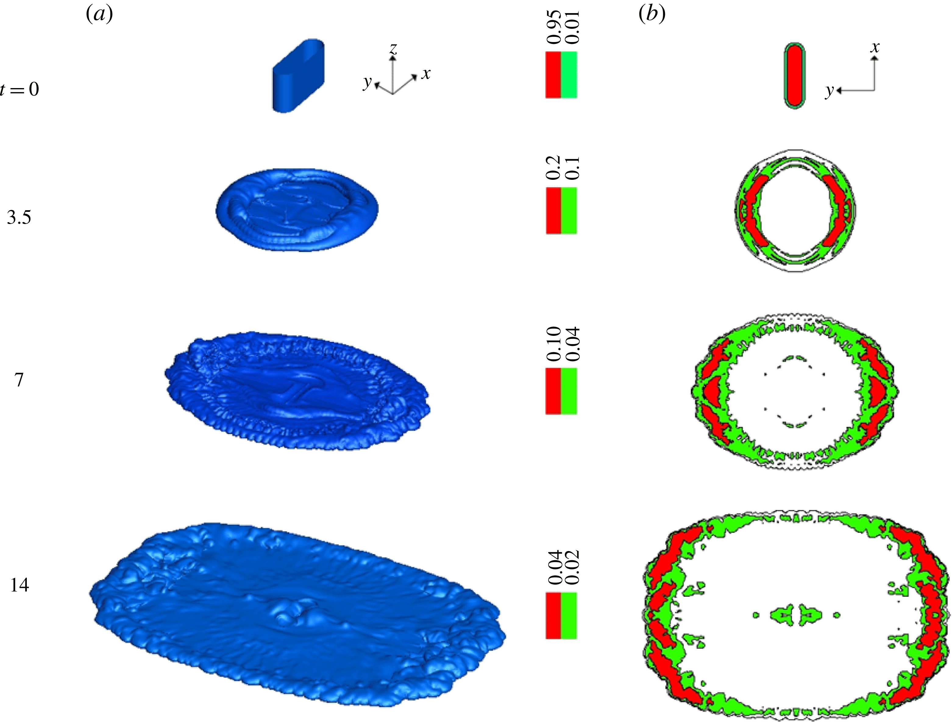
plan-view images (see figure 2), the maximum height of the current is located close to the front, in the ‘head’ of the gravity current. Note that this is in line with the recent laser-induced fluorescence measurements of Sahuri et al. (Reference Sahuri, Kaminski, Flynn and Ungarish2015) (see figure 4 in their paper). Therefore, it is reasonable to consider that the observed thickness in figure 5 (especially along the minor axis) corresponds to the front height of the current as opposed to that of the interior body of the current, which is significantly smaller, and hence hidden in the snapshots of figure 5. The same RR configuration was simulated, and in figure 6(a) we present the current’s height evolution via isosurfaces of density. In figure 6(b), we display the corresponding contours of the current height. Similar to the experimental findings, the heavy fluid is observed to aggregate along its periphery, with a clear distinction in thickness of approximately a factor of two between the minor and major axes. It is in fact this height inhomogeneity that leads to local velocity variations.
Side views of the (a) rounded rectangular and (b) circular gravity currents: (a) Exp 2 initial shape; (b) Exp 1 initial shape. Contrary to the RR release, the current’s thickness is roughly uniform for the circular release during spreading.

Height of the RR gravity current (Sim 1). (a) Isosurfaces
 ${\it\rho}=10^{-2}$
. (b) Distribution of the height along the horizontal plane. Note that the local height strongly varies along the circumference of the current, being maximum along the
 $y$
direction.

The present simulation results enable us to compare the value of the local Froude number along the front and specifically at the slow and fast sections of the fronts. One may assess the relevance of the various Froude functions reported in the literature with respect to the propagation of non-circular gravity currents. The simulations give access to local instantaneous front height
 $h_{N}$
and velocity
 $u_{N}$
information, and hence allow us to compute the Froude number as
 $\mathit{Fr}=u_{N}/\sqrt{h_{N}}$
. In order to evaluate the height
 $h_{N}$
for the slow and fast fronts, first the local height of the current,
 $h$
, is defined as
 $$\begin{eqnarray}h(x,y)=\int _{0}^{H}{\it\rho}\,\text{d}z.\end{eqnarray}$$
This local current height is then averaged over a wedge of
 $5^{\circ }$
aligned along the
 $x$
(slow front) and
 $y$
(fast front) axes, the averaging being performed over a distance extending between the front of the current and the location of the maximum height in the head.
The instantaneous local Froude number
 $\mathit{Fr}=u_{N}/\sqrt{h_{N}}$
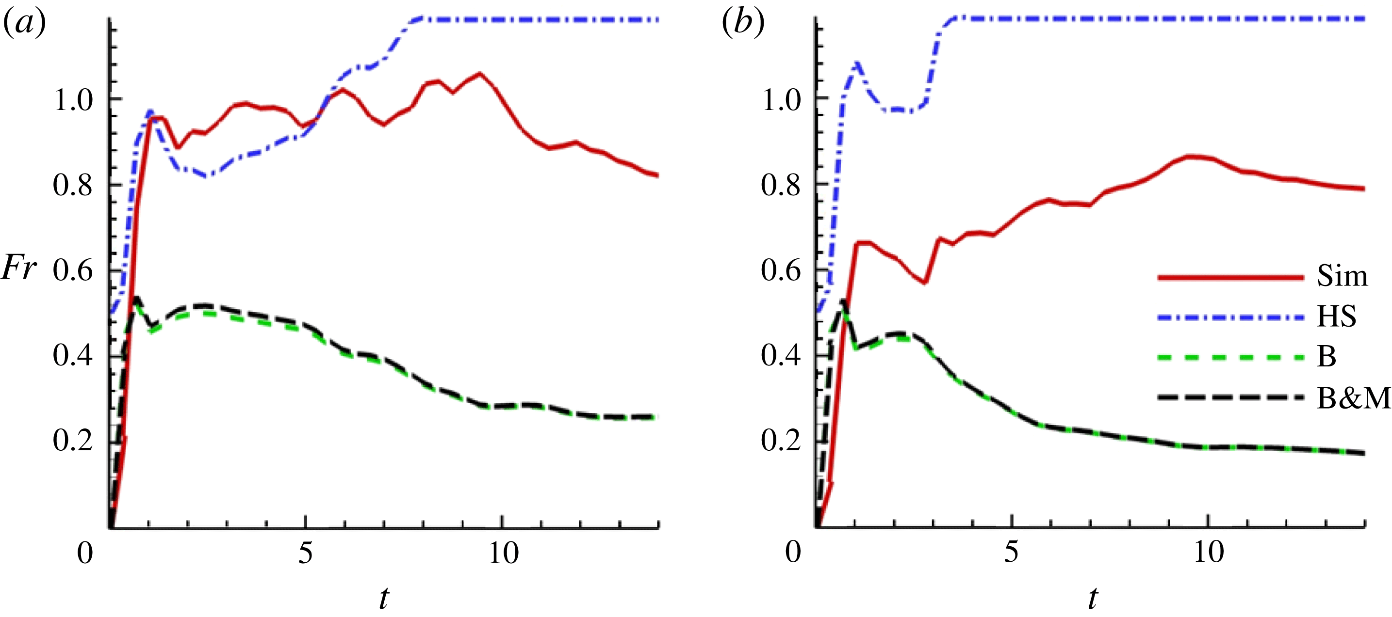
of the slow and fast sections of the front of an initially rounded rectangular release is plotted in figure 7. The fast front Fr fluctuates in the range 0.9–1.1 for
 $2\leqslant t\leqslant 10$
and decreases to approximately 0.7 at later times (in the self-similar inertial regime). On the contrary, the slow front Fr is significantly lower at early times (in the range 0.6–0.8 for
 $2\leqslant t\leqslant 10$
) but seems to catch up with the fast front at later times, i.e.
 $\mathit{Fr}\approx 0.7$
for
 $t>10$
. The larger value of the fast front Fr as compared to that of the slow front during the early stage of spreading suggests that the increase in front velocity due to mass redistribution inside the current is larger than the increase of height. Conversely, at late times (here
 $t>10$
) the evolutions of the front velocity and height are similar for both the fast and slow fronts, as the values of the local Froude number are roughly similar. This is in line with the fact that the current has entered the self-similar inertial phase.
Time evolution of the local Froude number at (a) the fast front and (b) the slow front:
 $\mathit{Fr}=u_{N}/\sqrt{h_{N}}$
, Sim 1 (——);
 $\mathit{Fr}^{HS}(a)=\min (a^{-1/3},1.19)$
(-
 $\cdot$
-
 $\cdot$
-);
 $\mathit{Fr}^{B}(a)=\sqrt{a(1-a)(2-a)/(1+a)}$
(- - - -);
 $\mathit{Fr}^{BM}(a)=\sqrt{2a}(1-a)$
(– – –). Here,
 $a$
is defined as
 $a=h_{N}/H$
.

Numerical simulations can also be used to evaluate the other models of Froude functions. These models generally depend on the ratio
 $a=h_{N}/H$
of the nose height of the current to that of the ambient. We consider in the following three models of Froude functions, namely Benjamin’s (Reference Benjamin1968) front condition
 $$\begin{eqnarray}\mathit{Fr}^{B}(a)=\sqrt{\frac{a(1-a)(2-a)}{(1+a)}},\end{eqnarray}$$
which is valid for
 $a\leqslant 1/2$
, Huppert & Simpson’s (Reference Huppert and Simpson1980) relation
 $$\begin{eqnarray}\mathit{Fr}^{HS}(a)=\min (0.5a^{-1/3},1.19)\end{eqnarray}$$
and Borden & Meiburg’s (Reference Borden and Meiburg2013) circulation-based model, which reads
 $$\begin{eqnarray}\mathit{Fr}^{BM}(a)=\sqrt{2a}(1-a).\end{eqnarray}$$
The Benjamin and BM models give almost identical results and consistently underpredict the local Froude number by approximately 50 %. Alternatively, the HS correlation is in reasonable agreement with the simulated fast front Froude number, but overestimates the slow front Froude number by approximately 30 % for the whole duration of spreading. It should be noted that good agreement cannot be expected for this comparison as the above Froude models were derived for quasi-steady two-dimensional currents, which is not the case for the present set of experiments and simulations. In addition, the models assume a hydrostatic flow (i.e. a gravity current that is long and thin), which is not necessarily the case for early times in the present experiments and simulations.
4. Extended box model simulations
Zgheib et al. (Reference Zgheib, Bonometti and Balacandar2014) proposed an extension of the box model initially developed by Huppert & Simpson (Reference Huppert and Simpson1980), capable of capturing the dynamics of non-axisymmetric gravity currents. Here we use this EBM to investigate the long-time inertial self-similar dynamics of non-axisymmetric currents.
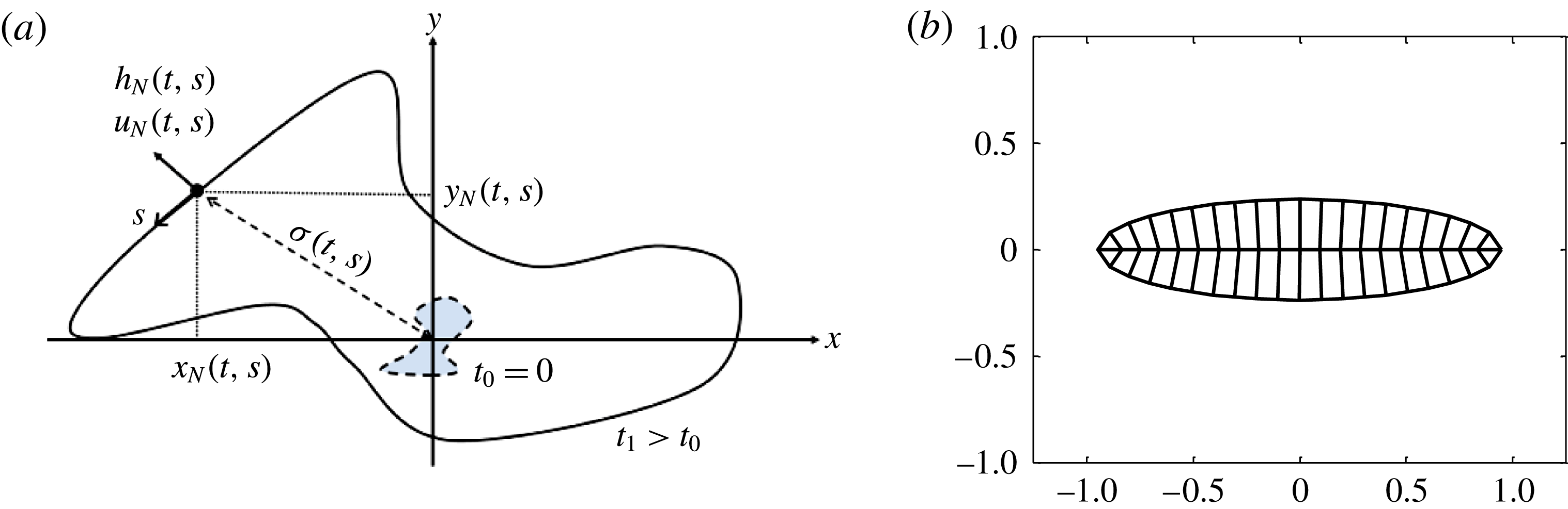
(a) Notation used for the two-dimensional EBM:
 $\{x_{N}(s,t),y_{N}(s,t)\}$
denote the local position,
 $h_{N}(s,t)$
the height,
 $u_{N}(s,t)$
the outward normal velocity of the front and
 ${\it\sigma}(s,t)$
the area per arclength. The independent variables
 $s$
and
 $t$
denote the curvilinear coordinate along the front and time, respectively. (b) Example of initial partitioning of the initial elliptical body of a non-axisymmetric gravity current.

4.1. Equations and assumptions
The classical box model generally used for predicting the evolution of gravity currents (Huppert & Simpson Reference Huppert and Simpson1980; Dade & Huppert Reference Dade and Huppert1995) has been shown to reproduce admirably the dynamics of axisymmetric and planar releases (see e.g. Ungarish & Zemach Reference Ungarish and Zemach2005). In the case of finite releases, the box model assumes the fluids to be immiscible, with negligible entrainment with the ambient, so that the mass and volume of the current are conserved throughout the duration of spreading. Additionally, the height is taken to be uniform along the body of the current and the current is advanced outwards normal to the front with a velocity proportional to the square root of the height. According to this model, the height intrinsically remains uniform along the circumference of the patch, so the speed of propagation is uniform along the current’s front during all phases of spreading. Therefore, using the classical box model, an initially non-axisymmetric current inevitably becomes axisymmetric.
The EBM proposed by Zgheib et al. (Reference Zgheib, Bonometti and Balacandar2014) is based on the partitioning of the initial release using inward rays normal to the front. An example of such partitioning is given in figure 8(b). Here, each segment of the front is now associated with a sub-volume of initial release. Once the various sub-volumes are obtained, the same procedure as in the classical box model is applied locally for each sub-volume, where the front is advanced outwards normal to itself. More particularly in the EBM, the current is defined by the front position
 $\{x_{N}(s,t),y_{N}(s,t)\}$
, the height
 $h_{N}(s,t)$
and the outward normal front velocity
 $u_{N}(s,t)$
, where
 $s$
is the distance measured along the circumference of the front. An additional variable, namely the area per arclength
 ${\it\sigma}(s,t)$
, is also used in the model (figure 8
a). An integration of
 ${\it\sigma}(s,t)$
over the entire arclength of the advancing front yields the total area covered by the planform of the advancing current. The EBM can be summarized by the following set of coupled equations (Zgheib et al.
Reference Zgheib, Bonometti and Balacandar2014):
 $$\begin{eqnarray}u_{N}=\mathit{Fr}\sqrt{h_{N}},\quad \mathit{Fr}=\min (0.5h_{N}^{-1/3},1.19),\end{eqnarray}$$
 $$\begin{eqnarray}\displaystyle & \displaystyle \left\{\frac{\partial x_{N}}{\partial t},\frac{\partial x_{N}}{\partial t}\right\}=u_{N}\frac{\{\partial y_{N}/\partial s,-\partial x_{N}/\partial s\}}{\sqrt{(\partial x_{N}/\partial s)^{2}+(\partial y_{N}/\partial s)^{2}}}, & \displaystyle\end{eqnarray}$$
 $$\begin{eqnarray}\displaystyle & \displaystyle \frac{\partial {\it\sigma}}{\partial t}=u_{N}, & \displaystyle\end{eqnarray}$$
 $$\begin{eqnarray}\frac{\partial {\it\sigma}h_{N}}{\partial t}=0,\end{eqnarray}$$
where
 $\mathit{Fr}$
is the Froude number, which is here calculated from the Huppert & Simpson (Reference Huppert and Simpson1980) empirical relation. Note that any other model of Froude-number function could be used without loss of generality, provided this function is applicable for the whole range of height ratio of nose to ambient,
 $h_{N}/H$
, considered here. All variables are dimensionless. Equations (4.1)–(4.3) refer to the Froude front condition, kinematic relations and mass conservation, respectively. In (4.2a
), the current is restricted to normal outward spreading with velocity
 $u_{N}$
. It will be shown below that this is a good approximation despite the non-uniform height distribution along the front, which might induce a tangential velocity component. The increase in the current’s surface area is captured in (4.2b
). This step is non-existent in the classical box model, as the area increase can be directly inferred from the radius of the current.
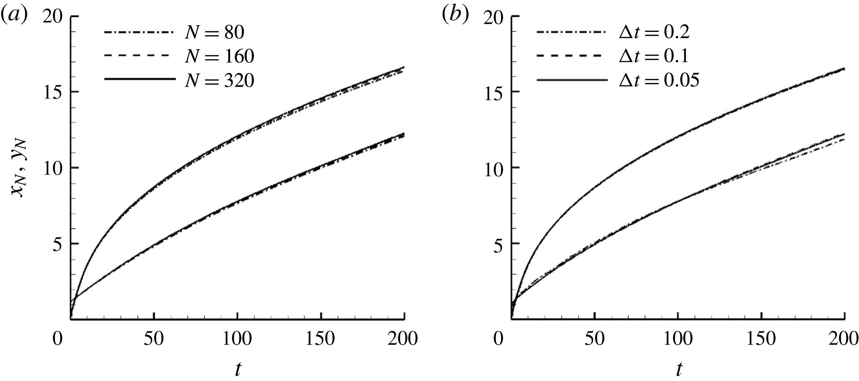
Analytical solutions of (4.1)–(4.3) are not feasible in the case of arbitrary initial patches. However, the system may be solved numerically. Details of the numerical procedure used for solving (4.1)–(4.3) and verification of spatial and temporal convergence are given in appendix A.
4.2. Examination of the extended box model
The EBM involves various approximations that can be summarized as follows. (H1) The volume of initial release is partitioned with the help of inward-propagating (normal to the front) geometric rays, and accordingly different sub-volumes are assigned to the different portions of the front. (H2) As the current propagates, the height of the current is not taken to be constant over the entire release. It varies along the front depending on the local speed of propagation. (H3) The velocity of propagation is taken to be normal to the front. Since there is variation in the height of the current along the front, it can be expected that there is some cross-flow (tangential velocity) induced by this variation in the current height. However, since the pressure gradient normal to the front is expected to greatly exceed the tangential gradient at the front, the current velocity is likely to be predominantly normal to the front. (H4) Finally, we assume that, even in the present case of non-axisymmetric propagation, the Huppert–Simpson front relation can be used to express the front velocity in terms of local front height. Here we examine these assumptions relative to the results of fully resolved simulations.
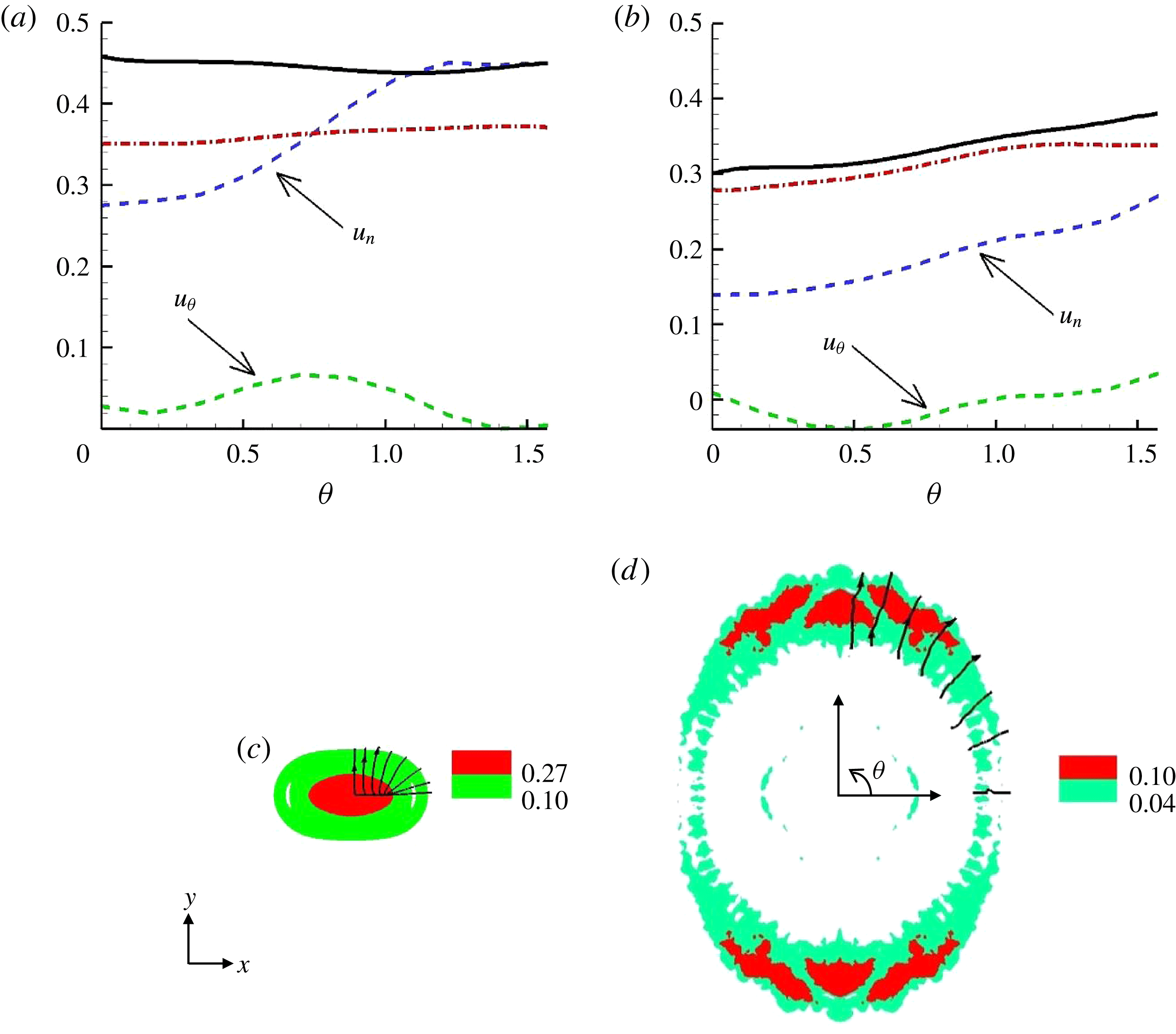
(a,b) Azimuthal evolution of the normal-to-the-front
 $u_{n}$
and tangential component
 $u_{{\it\theta}}$
of the front velocity of a rounded rectangular gravity current at two different time instants (Sim 1). Also plotted is the velocity obtained via the Huppert & Simpson (Reference Huppert and Simpson1980) Froude function (see (3.9)) using the mean height (dash-dotted red line) and the maximum height (solid black line) in the head of the current extracted from the fully resolved simulation. (c,d) Height distribution in the RR current before and after the switch of axes at
 $t=1.5$
and
 $t=7$
, respectively. The streamlines of the vertically averaged velocity field in the current are also plotted in the upper right corner.

Let us first examine the direction of fluid velocity at the front of the current. To focus on the velocity of the outward-propagating current and eliminate the contribution from the inward-propagating ambient, we define the depth-averaged velocity of the current as follows:
 $$\begin{eqnarray}\bar{u}=\frac{\displaystyle \int _{0}^{H}{\it\rho}u\,\text{d}z}{\displaystyle \int _{0}^{H}{\it\rho}\,\text{d}z},\quad \bar{v}=\frac{\displaystyle \int _{0}^{H}{\it\rho}v\,\text{d}z}{\displaystyle \int _{0}^{H}{\it\rho}\,\text{d}z}.\end{eqnarray}$$
Recall that
 ${\it\rho}=1$
in the current and
 ${\it\rho}=0$
in the ambient. From (4.4), one can extract the velocity along the front and compute the normal-to-the-front and tangential components of the front velocity
 $u_{n}$
and
 $u_{{\it\theta}}$
as plotted in figure 9. The simulation results indicate that the normal velocity is an order of magnitude larger than the tangential component of velocity over the entire front of the current. Furthermore, the faster propagation of the current along the
 $y$
axis (
 ${\it\theta}={\rm\pi}/2$
) is clear. Integrating over the entire front, we find the average normal-to-the-front and tangential front velocities to be approximately 0.37 (0.19) and 0.03 (0.03) at
 $t=1.5$
(7), respectively. Interestingly, the tangential velocity is mostly positive at
 $t=1.5$
(when the height is nearly uniform), indicating a slight cross-flow towards the fast front and initial accumulation of excess material at the fast front. Alternatively,
 $u_{{\it\theta}}$
is mostly negative at
 $t=7$
(when the height is much larger at the fast front), in line with the expectation that there may be some cross-flow induced by the hydrostatic pressure gradient stemming from the variation in the current height. Overall, this corroborates approximation H3. Secondly, approximation H2 can be readily verified thanks to figures 5(a) and 6(b), which show that the height of the current is not homogeneous along the front during spreading.
We also present in figure 9 the normal-to-the-front velocity estimated by Huppert & Simpson’s (Reference Huppert and Simpson1980) front Froude-number relation using both the head of the current’s mean height and the maximum height taken from the simulation. At the early time
 $t=1.5$
, reasonable agreement is observed between the simulation results and the prediction. However at
 $t=7$
, the HS prediction is significantly larger by 45 % than the simulation results. It is noteworthy that, even though the simulated front velocity in the present case is consistently lower than the HS prediction, the EBM with the HS front velocity is capable of predicting the front motion reasonably well (Zgheib et al.
Reference Zgheib, Bonometti and Balacandar2014). This is not a contradiction: in the box model, the height of the current is underpredicted since the current is taken to be of uniform height. This underprediction of the front height somewhat compensates the presently observed overestimation of the front velocity given by the Huppert and Simpson Froude-number relation.
Two snapshots of the height distribution of the rounded rectangular release are presented in figure 9(b) together with streamlines (evaluated from the vertically averaged velocity defined in (4.4)). At early times, the streamlines resemble the inward-propagating geometric rays (which are normal to the front) shown in figure 8(b). At later times, the streamlines remain preferentially normal to the front. This is consistent with the earlier observation that the velocity of the current is dominantly oriented along the normal direction. This also provides some support for approximation H1 that the initial partitioning of the release volume is dictated by the inward-propagating geometric rays normal to the front.
4.3. A scaling law for the final shape of non-circular gravity currents
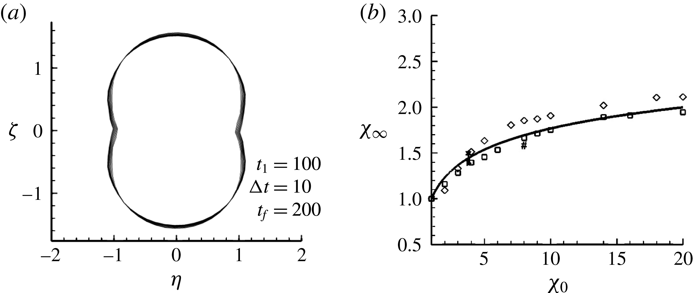
Scaling laws for flows such as turbulent jets, plumes and gravity currents under complex conditions such as cross-flow ambient are important for evaluating particular flow configurations (List Reference List1982). In this section we use the EBM to analyse the characteristic self-similar development of a non-axisymmetric gravity current. As shown earlier by experiments, an initially non-circular gravity current eventually reaches an inertial self-similar shape that is non-axisymmetric. Figure 10(a) presents the evolution of the front obtained from an EBM calculation for an initially elliptical release. Here, the initial length of the major and minor axes of the ellipse are 0.90 and 0.24, respectively. These dimensions correspond to an initial horizontal aspect ratio of
 ${\it\chi}_{0}\approx 3.8$
and a vertical aspect ratio of
 ${\it\lambda}\approx 2$
. We show 11 contours of the front in the (
 ${\it\eta}=xt^{-1/2}$
,
 ${\it\zeta}=yt^{-1/2}$
) plane from an initial non-dimensional time of
 $t=100$
to a final time of
 $t=200$
with a time increment of
 ${\rm\Delta}t=10$
. Clearly, the current has reached a near self-similar shape.
(a) Evolution of the front contour of an initially elliptical release of horizontal initial aspect ratio
 ${\it\chi}_{0}=3.8$
in the (
 ${\it\eta}=xt^{-1/2}$
,
 ${\it\zeta}=yt^{-1/2}$
) plane obtained from an EBM simulation. Here, the contours are plotted from
 $t_{0}=100$
to
 $t_{f}=200$
in steps of
 ${\rm\Delta}t=10$
. (b) Self-similar horizontal aspect ratio
 ${\it\chi}_{\infty }$
of the front contour of non-axisymmetric gravity currents as a function of the horizontal initial aspect ratio
 ${\it\chi}_{0}$
: ▾, ◂, ▸, experiments 2, 3, 4, respectively;
 $\ast$
, ○,
 $\#,+$
, fully resolved simulations 1, 2, 3, 4 respectively; ▫, ♢, EBM simulations with releases of initially elliptical and rounded rectangular shape, respectively; ——, correlation
 ${\it\chi}_{\infty }=1+(\ln {\it\chi}_{0})/3$
.

We performed a series of calculations with the EBM where the initial horizontal aspect ratio
 ${\it\chi}_{0}$
of the non-axisymmetric gravity current was varied in the range
 $1\leqslant {\it\chi}_{0}\leqslant 20$
. For each
 ${\it\chi}_{0}$
case, the self-similar aspect ratio
 ${\it\chi}_{\infty }$
was measured. To be specific, we take the value of
 ${\it\chi}_{\infty }$
at a sufficiently large time, here
 $t=200$
, so the self-similar regime was reached. EBM calculations were performed for two initial non-circular shapes, namely elliptical and rounded rectangular shapes. The EBM results are summarized in figure 10(b). For comparison, we also plotted the results obtained by the experiments and simulations of table 1. All the data roughly follow a similar trend, which can be modelled by the following simple empirical relation:
 $$\begin{eqnarray}{\it\chi}_{\infty }=1+{\textstyle \frac{1}{3}}\ln {\it\chi}_{0}.\end{eqnarray}$$
In the case of a circular release, it can be shown that the temporal evolutions of the front height
 $h_{N}$
, radius
 $r_{N}$
and normal-to-the-front velocity
 $u_{N}$
in the inertial self-similar regime scale as
 $t^{2{\it\alpha}}$
,
 $t^{-{\it\alpha}}$
and
 $t^{{\it\alpha}}$
with
 ${\it\alpha}=-1/2$
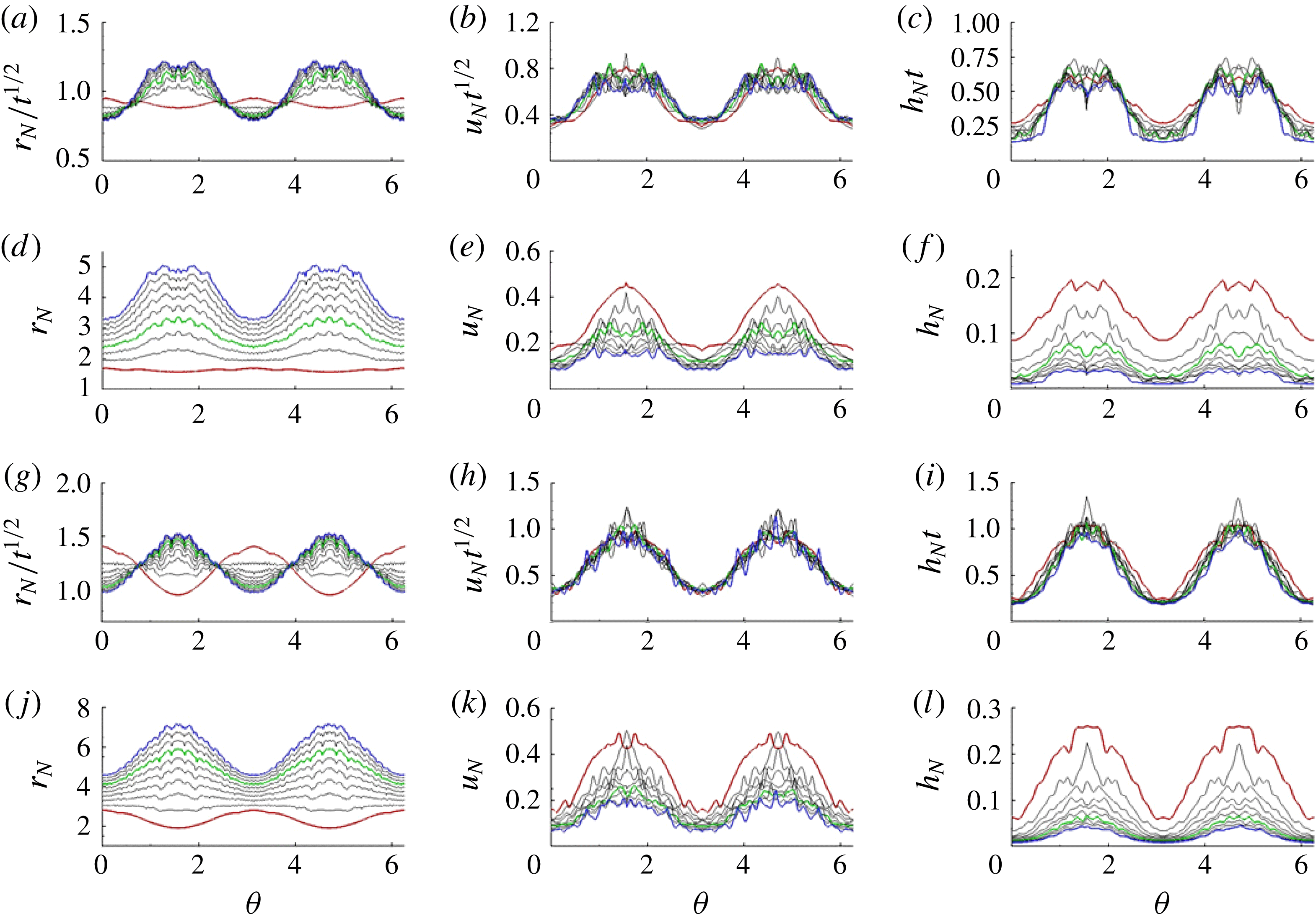
(see e.g. Ungarish Reference Ungarish2009, p. 122). Figure 11 displays the azimuthal variation of the front height, radius and normal-to-the-front velocity using the aforementioned scaling from Sim 1 (
 ${\it\chi}_{0}=3.8$
) and Sim 3 (
 ${\it\chi}_{0}=8$
). Here
 ${\it\theta}$
is the angle measured anticlockwise from the
 $x$
axis. We observe that the normalized
 $r_{N}$
,
 $u_{N}$
and
 $h_{N}$
for both simulations reach a self-similar profile that resembles a sinusoidal curve. This suggests that the function
 $f({\it\theta})$
introduced in (3.1)–(3.3) may be written as
 $f({\it\theta})=1+g({\it\theta})$
, with
 $g({\it\theta})$
being a sinusoidal function to be determined. For Sim 1 (
 ${\it\chi}_{0}=3.8$
), we plot the azimuthal dependence of radius, speed and height from
 $t=3.15$
(red curve) to
 $t=17.15$
(blue curve) with a constant time increment of
 ${\rm\Delta}t=1.75$
. The green curve at
 $t=8.4$
represents the time at which these quantities become roughly self-similar. Similarly for Sim 3 (
 ${\it\chi}_{0}=8$
), we plot the azimuthal evolution from
 $t=4$
(red curve) to
 $t=22$
(blue curve) with a constant time increment of
 ${\rm\Delta}t=2$
. The green curve at
 $t=16$
represents the time beyond which these quantities become roughly self-similar. Beyond the self-similar phase, the height, speed and radius are observed to attain a minimum value at
 ${\it\theta}=0,{\rm\pi}$
and
 $2{\rm\pi}$
, and a maximum value at
 ${\it\theta}={\rm\pi}/2$
and
 $3{\rm\pi}/2$
. This self-similar shape is indicative of an elliptical like shape whose minor axis coincides with the
 ${\it\theta}=0$
line, which corresponds to the
 $x$
axis in the
 $x$
–
 $y$
plane.
Evolution for
 ${\it\chi}_{0}=3.8$
(Sim 1) of the front contours (a,d), front speed (b,e) and mean front height (c,f). The contours are plotted from
 $t_{0}=3.15$
(red curve) to
 $t_{f}=17.15$
(blue curve) in steps of
 ${\rm\Delta}t=1.75$
. Plotted in green is the curve corresponding the time
 $t=8.4$
for which these quantities become roughly self-similar. Evolution for
 ${\it\chi}_{0}=8$
(Sim 3) of the front contours (g,j), front speed (h,k) and mean front height (i,l). The contours are plotted from
 $t_{0}=4$
(red curve) to
 $t_{f}=22$
(blue curve) in steps of
 ${\rm\Delta}t=2$
. Plotted in green is the curve corresponding the time
 $t=16$
for which these quantities become roughly self-similar.

Subtracting the mean value from each curve, the scaled radius (
 $r_{N}t_{f}^{-1/2}$
), front speed (
 $u_{N}t_{f}^{1/2}$
) and front height (
 $h_{N}t_{f}$
) may be approximately described by a single sinusoidal function of the form
 $$\begin{eqnarray}g({\it\theta})=-A\cos (2{\it\theta}+{\it\theta}_{0}),\end{eqnarray}$$
where
 $A$
and
 ${\it\theta}_{0}$
represent the amplitude and phase angle, respectively. The phase angle
 ${\it\theta}_{0}$
is the angle the
 $x$
axis makes with the major axis of the rounded rectangle and, in the present case,
 ${\it\theta}_{0}=0$
. The amplitude
 $A$
is obtained from the average root mean square (r.m.s.) value of the three curves (radius, speed and height) as
 $A\approx 0.22$
for Sim 1 and
 $A\approx 0.32$
for Sim 3, for which
 ${\it\chi}_{0}=3.8$
and 8, respectively. Since
 $A$
is obviously 0 for
 ${\it\chi}_{0}=1$
, the present results indicate that
 $A$
increases as
 ${\it\chi}_{0}$
is increased, i.e. the larger the non-axisymmetry of the initial release, the higher the contrast of the front height and speed along the front contour. This is in line with (4.5), which predicts a larger self-similar aspect ratio for larger initial horizontal aspect ratios. In fact, we found that the amplitude
 $A$
of
 $g({\it\theta})$
can be nicely described by the empirical relation
 $A\approx (\ln {\it\chi}_{0})/6$
, at least for the three values of
 ${\it\chi}_{0}$
used in the simulations (namely
 ${\it\chi}_{0}=1,3.8$
and 8). As for the EBM data, an empirical relation of the form
 $A\approx (2/9)\ln {\it\chi}_{0}$
provides a better fit in the range
 ${\it\chi}_{0}=[1,20]$
. Note that, in computing
 $A$
from the EBM, the values from the height were discarded since the height is consistently underpredicted (recall that the height of the current in the EBM is averaged over the entire sector, which is not the case in reality, as seen in figures 2 and 6).
In figure 12, we plot the azimuthal evolution at the end of each simulation for the scaled front location (
 $r_{N}t_{f}^{-1/2}$
), speed (
 $u_{N}t_{f}^{1/2}$
) and height (
 $h_{N}t_{f}$
), for which the mean value of each curve has been subtracted. We plot the results from Sim 1 and Sim 3 and observe good agreement between the three curves and the sinusoidal function
 $g({\it\theta})$
defined in (4.6). It follows that, with the knowledge of the self-similar shape of the front, one could roughly predict the front height (or front speed) of the current provided the front height (or front speed) is known at some azimuthal orientation.
Azimuthal evolution at the final time of the scaled front location (red solid), speed (green dashed) and height (blue dash-dotted) from (a) Sim 1 (
 ${\it\chi}_{0}=3.8$
) and (b) Sim 3 (
 ${\it\chi}_{0}=8$
). The thick solid black line corresponds to
 $f({\it\theta})$
from (4.6). The mean value is subtracted from each curve.

5. Effect of the initial vertical and horizontal aspect ratios
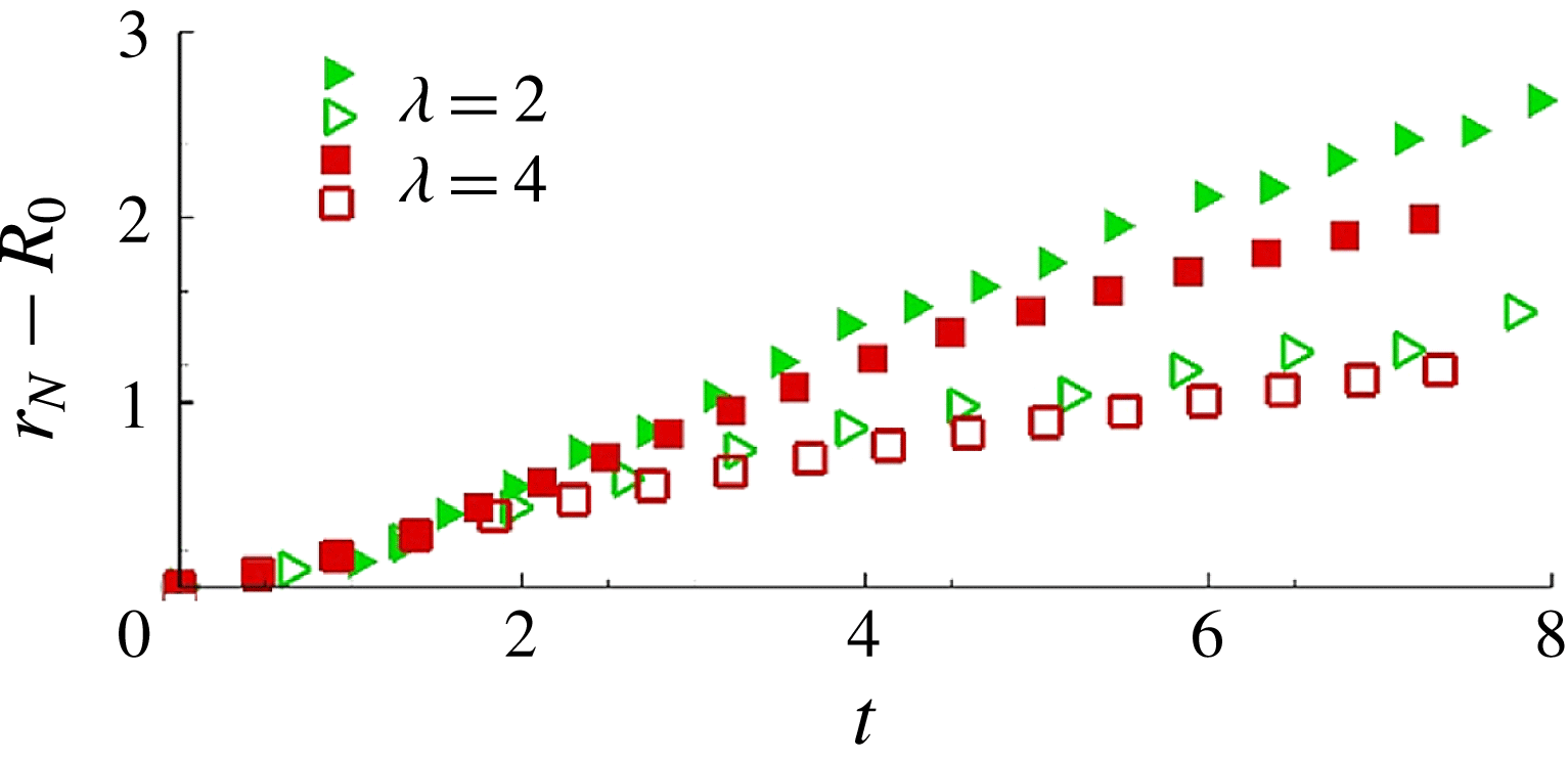
The dependence on the vertical aspect ratio is examined experimentally by doubling the vertical aspect ratio while maintaining the same density ratio. We present in figure 13 the same configuration for two initial vertical aspect ratios
 ${\it\lambda}=2$
and 4. The fast and slow fronts are again observed to change the orientation of the initial major and minor axes of the release. Other experiments with smaller vertical aspect ratios of 0.25 and 0.5 were also conducted, and the same preferential direction of spreading and switching of major and minor axes was always observed. We may conclude that the switching of the initial major and minor axes is not sensitive to the vertical aspect ratio, at least in the range
 $0.25\leqslant {\it\lambda}\leqslant 4$
.
Time evolution of the fast front (solid symbols) and slow front (open symbols) of a RR release of initial vertical aspect ratio: ▹, ▸,
 ${\it\lambda}=2$
, Exp 2; and ▫,
 $\blacksquare$
,
 ${\it\lambda}=4$
, Exp 5.

We use results from Sim 1 (
 ${\it\chi}_{0}=3.8$
) and Sim 3 (
 ${\it\chi}_{0}=8$
) of the RR geometry to investigate the effect of the horizontal aspect ratio
 ${\it\chi}_{0}$
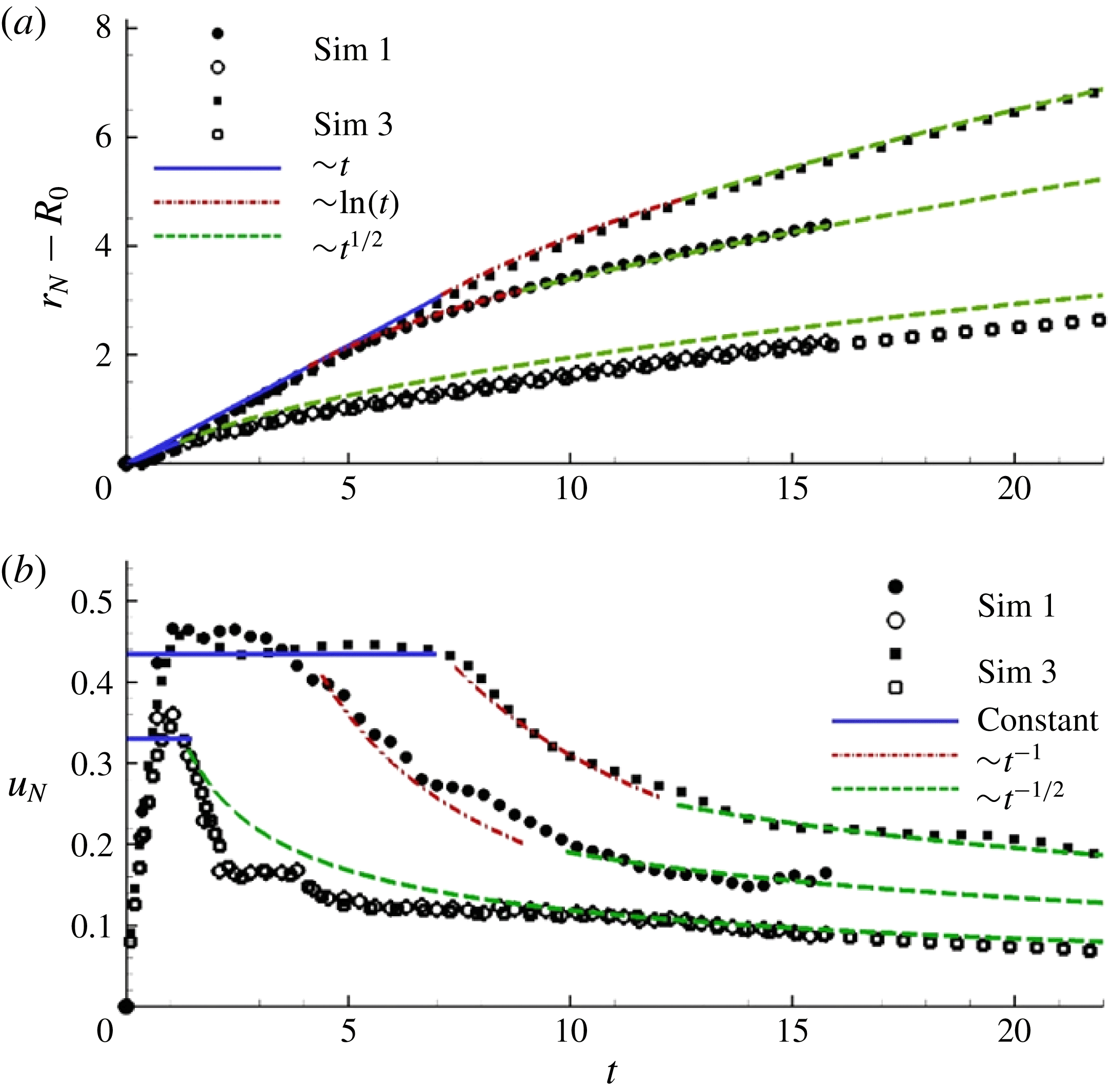
on the front dynamics. Note that the initial shape of the RR in Sim 3 has the same height and width as that of Sim 1, but its length is 2.1 times larger. In figure 14(a), we plot the time evolution of the front position
 $(r_{N}-R_{0})$
along the fast (
 $y$
axis) and slow (
 $x$
axis) fronts from Sim 1 and Sim 3. The corresponding front velocity
 $u_{N}$
is shown in figure 14(b).
(a) Temporal evolution of the fast (filled symbols) and slow (open symbols) fronts from Sim 1 (circles) and Sim 3 (squares). The solid blue, dash-dotted red and dashed green lines are obtained from (b) by integrating the corresponding front velocity curves. (b) Fast front (filled symbols) and slow front (open symbols) velocities from Sim 1 (circles) and Sim 3 (squares). The solid blue, dash-dotted red and dashed green lines represent the constant-velocity slumping, fast decay
 ${\sim}t^{-1}$
and axisymmetric inertial-like decay
 ${\sim}t^{-1/2}$
phases, respectively.

Along the
 $x$
axis, the distance travelled by the slow-moving front (open symbols in figure 14(a)), and consequently the corresponding front velocity (open symbols in figure 14(b)), for both simulations are found to agree well with one another for the entire duration of spreading, including the acceleration phase (
 $0<t\lesssim 1$
) and the deceleration phase (
 $t\geqslant 1$
). This near-perfect agreement implies that the front dynamics along the
 $x$
axis is unaffected by the increase in the length of the RR from Sim 1 to Sim 3, as none of this additional fluid contributes to the front dynamics along the
 $x$
axis. Furthermore, the present agreement allows us to conjecture that the current, along the
 $x$
axis, behaves like that pertaining to a circular release of the same initial non-dimensional height (
 $h_{0}=1$
) as that of the RR, but with an initial radius equivalent to half the width of the RR, i.e.
 $R_{0}=0.24$
(for Sim 1 and 3,
 $R_{0}=0.48$
). To test this hypothesis, we calculate the front speed of a circular release (of initial height and radius
 $h_{0}=1$
and
 $R_{0}=0.24$
, respectively) from established theoretical predictions. The asymptotic behaviour of the front velocity of an axisymmetric current in the inertial phase is given by (Fannelop & Waldman Reference Fannelop and Waldman1971; Hoult Reference Hoult1972; Huppert & Simpson Reference Huppert and Simpson1980; Rottman & Simpson Reference Rottman and Simpson1983)
 $$\begin{eqnarray}u_{N}={\textstyle \frac{1}{2}}{\rm\pi}^{1/4}{\it\xi}_{c}h_{0}^{1/4}\sqrt{R_{0}/t}.\end{eqnarray}$$
The non-dimensional transition time from the slumping to the inertial spreading phase (
 $t_{SI}$
) can be estimated via (2.2). Using the slumping velocity of the current of Sim 1 immediately following the end of the acceleration phase, namely
 $F_{c,sl}\approx 0.33$
, we find
 $t_{SI}\approx 1.3$
, using the value of
 ${\it\xi}_{c}=1.16$
suggested by Huppert & Simpson (Reference Huppert and Simpson1980). This is in agreement with the observed transition time, which is roughly unity. The proposed asymptotic front velocity (5.1) is observed to agree well with the velocity of the slow front obtained from Sim 1 and Sim 3 (see figure 14
b). This reinforces the proposition that the slow-moving front behaves as an axisymmetric current whose initial radius is equivalent to half the width of the RR.
The dynamics along the
 $y$
axis is more complicated. Here we conjecture that the fast front initially advances as a planar (lock-release) current of initial non-dimensional height (
 $h_{0}=1$
) like that of the RR and with an initial lock length equivalent to half the width of the RR release. This planar spreading is likely to continue up to a time
 $t_{PF}$
defined as the time instant from which the front velocity significantly decreases. This time, which seems to be proportional to the initial horizontal aspect ratio
 ${\it\chi}_{0}$
, is not known a priori but can be estimated from the temporal evolution of the front velocity in figure 14(b).
The velocity of the fast front (along the
 $y$
axis) of both simulations is seen to transition through four phases. (i) First there is a brief initial acceleration phase (
 $0<t\lesssim 1$
), at the end of which the front attains its maximum speed. (ii) Then there is a planar slumping phase characterized by a constant velocity, and whose duration varies depending on the initial horizontal aspect ratio
 ${\it\chi}_{0}$
. The planar slumping phase is identified by the solid blue line in figure 14. (iii) There follows a fast decay phase where the velocity scales as
 $t^{-1}$
. The duration and transition into and out of this phase depend again on
 ${\it\chi}_{0}$
. This phase is identified by the red dot-dashed line in figure 14. (iv) Finally, an axisymmetric-like inertial phase follows, where the velocity decays as
 $t^{-1/2}$
. This power-law decay is usually observed during the inertial self-similar phase of an axisymmetric release. It is indicated by the green dashed line in figure 14. Here, again, the duration and transition into this phase depend on
 ${\it\chi}_{0}$
. We denote by
 $t_{FC}$
the non-dimensional transition time between the fast decay (dash-dotted red line) and the axisymmetric inertial (dashed green line) spreading modes.
The first two phases of spreading, namely the acceleration and the constant-velocity slumping phases, are usually observed in planar lock-release gravity currents. The front velocities from both simulations are in good agreement during these phases up to a time of
 $t\approx 4$
when the front velocity from Sim 1 (
 ${\it\chi}_{0}=3.8$
) transitions into the fast decay phase. This transition time is denoted by
 $t_{PF}$
. Similarly for Sim 3 (
 ${\it\chi}_{0}=8$
) we observe
 $t_{PF}\approx 7$
. It should be noted that the present velocity decay, scaling as
 $t^{-1}$
during
 $t_{PF}\leqslant t\leqslant t_{FC}$
, is sharper than in the classical inertial phase of a planar current, for which the front velocity scales as
 $t^{-1/3}$
. The fast front remains in the fast decay phase for approximately five non-dimensional time units before transitioning into the axisymmetric inertial spreading phase. This transition time occurs roughly around
 $t_{FC}=9.0$
and
 $t_{FC}=12.6$
for Sim 1 and Sim 3, respectively.
In both RR simulations, the transition from a planar to a ‘finite-release’ faster decay occurs when the fast front is still in the slumping (constant-velocity) phase. This may be because, in both cases, the initial aspect ratio of the RR release is smaller than a critical length needed for the fast front to transition from the planar slumping to the planar inertial phase of spreading. This planar slumping to planar inertial transition time,
 $t_{SI}$
, may be estimated by matching the constant velocity during the slumping phase to the front velocity in the inertial phase of a planar lock-release current (Fannelop & Waldman Reference Fannelop and Waldman1971; Hoult Reference Hoult1972; Huppert & Simpson Reference Huppert and Simpson1980; Rottman & Simpson Reference Rottman and Simpson1983) and is given by
 $$\begin{eqnarray}t_{SI}=Y_{0}h_{0}({\it\xi}_{p}/F_{p,sl})^{3},\end{eqnarray}$$
where
 $Y_{0}$
is the initial dimensionless lock length (here,
 $Y_{0}=0.24$
) and
 $h_{0}=1$
is the initial height of the planar lock-release. The constant
 $F_{p,sl}$
corresponds to the constant velocity of the planar current in the slumping phase. Here
 $F_{p,sl}$
is obtained from the observed fast front velocity in the slumping phase, namely
 $F_{p,sl}\approx 0.44$
. The values of
 ${\it\xi}_{p}$
proposed by Hoult (Reference Hoult1972) and Huppert & Simpson (Reference Huppert and Simpson1980) are
 ${\it\xi}_{p}=1.6$
and
 ${\it\xi}_{p}=1.47$
, respectively. Depending on the chosen value of
 ${\it\xi}_{p}$
, the non-dimensional slumping to inertial transition time
 $t_{SI}$
falls in the range
 $9.2<t_{SI}<11.81$
. This predicted value of
 $t_{SI}$
is greater than
 $t_{PF}$
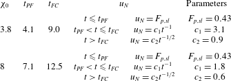
for both RR releases, and as a result the transition from planar to ‘finite-release’ faster decay occurs while the fast fronts are still in the planar slumping phase in both Sim 1 and Sim 3. Tables 2 and 3 summarize the various phases of spreading and transition times shown in figure 14.
The spreading phases and transition times for the fast front of Sim 1 and Sim 3 shown in figure 14(b).

The slumping and inertial front velocity phases and transition time for an axisymmetric release corresponding to the slow front of Sim 1 and Sim 3 shown in figure 14(b).

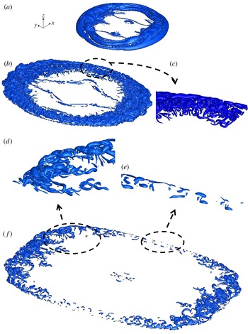
Isosurfaces of
 ${\it\lambda}_{ci}=2$
for the RR release (Sim 1) for (a)
 $t=3.5$
, (b,c)
 $t=7$
and (d–f)
 $t=14$
.

6. Vortical structure of non-circular/non-planar gravity currents
Shortly after release, the current intrudes into the ambient fluid, forming a smooth front in which Kelvin–Helmholtz rolled up vortices separate the body from the head of the current. The signature of these vortices is visible in the density isosurface plots of figure 6. The head of the current is complex and includes vortical structures that are not fully observable in the density isosurface plots, but are better identified in isosurface plots of the swirling strength
 ${\it\lambda}_{ci}$
in figure 15. The swirling strength is defined as the absolute value of the imaginary portion of the complex eigenvalue of the velocity gradient tensor. It is commonly used for identifying regions of intense vorticity (Zhou et al.
Reference Zhou, Adrian, Balachandar and Kendall1999; Chakraborty, Balachandar & Adrian Reference Chakraborty, Balachandar and Adrian2005; Cantero et al.
Reference Cantero, Balachandar and Garcia2007b
). The maximum, mean and r.m.s. values of
 ${\it\lambda}_{ci}$
at
 $t=3.5,~7$
and 14 are
 $\{65,0.020,0.34\}$
,
 $\{25,0.024,0.30\}$
, and
 $\{14,0.015,0.15\}$
, respectively. The swirling strength is highest at the head of the fast front of the current, where the flow is dominated by hairpin vortices and inclined vortical structures.
Vertically averaged
 ${\it\lambda}_{ci}$
over the height of the current for (a) axisymmetric release (Sim 2) and (b) RR release (Sim 1). The initial volume of the current is the same for both cases.

Owing to the preferential direction of spreading, the vortex tubes at the slow front, i.e. parallel to the
 $y$
axis, undergo stretching and twisting (figure 15
c) before they eventually break up into smaller structures (figure 15
e). In figure 16, the spatial distribution of the vertically averaged swirling strength reveals that the swirling strength at the fast front is as large as twice that at the slow front. Isosurfaces of
 ${\it\lambda}_{ci}$
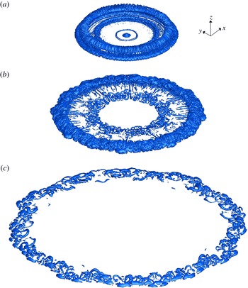
for a cylindrical release of equivalent volume are displayed in figure 17. For the sake of comparison, the maximum, mean and r.m.s. values of
 ${\it\lambda}_{ci}$
at
 $t=3.5,~7$
and 14 are
 $\{47,0.032,0.5\}$
,
 $\{39,0.038,0.41\}$
and
 $\{12,0.020,0.17\}$
, respectively. It is noteworthy that the mean value of
 ${\it\lambda}_{ci}$
is consistently larger in the circular case than in the rounded rectangular release. We conjecture that the observed higher intensity of the swirling strength is due to the fact that the initial axisymmetry of the circular release artificially increases the coherence of the vortex tubes since the local stretching field is likely to be more uniform in this case. In any case, the explanation of the present observation remains unclear at the present time.
Same as figure 15 for the cylindrical release (Sim 2): (a)
 $t=3.5$
; (b)
 $t=7$
; (c)
 $t=14$
.

7. Discussion
In this section, we present quantitative and qualitative results from additional experiments and simulations in which one parameter at a time was varied so that one may assess the robustness of the non-axisymmetric spreading of finite releases to a larger class of non-axisymmetric releases of material. We also present simulation results to further strengthen the experimental observation that the effect of the tank boundaries may be ignored.
7.1. Varying current-to-ambient density ratio
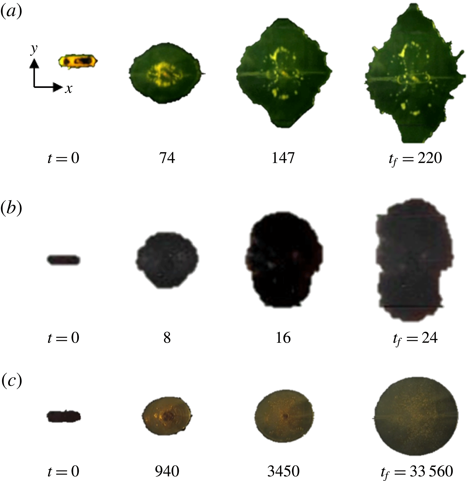
We investigate in figure 18(a) the case of a dam-break (water in air) flow of a heavy current of density ratio
 ${\it\rho}_{c}/{\it\rho}_{a}=10^{3}$
. At
 $t=74$
the initial major axis (
 $x$
coordinate) still remains the major axis of the spreading current, but by
 $t=147$
and later the current spreads faster along the
 $y$
direction. This flipping of axes is similar to what has been observed for the Boussinesq currents. Note that the global contour of the front is not as smooth as in the Boussinesq case (figure 4
b). At
 $t=147$
and 220 breakage of the front into smaller chunks can be observed. This is attributed to interactions between the front of the current and the bottom glass wall. At large density ratios, wall friction can significantly affect the front speed (Bonometti, Balachandar & Magnaudet Reference Bonometti, Balachandar and Magnaudet2008). The surface of the bottom wall in terms of degree of dryness and hence local variations of wall friction may have played a role in the experiment. In addition, capillary effects are likely to be significant at late times (
 $t\geqslant 100$
) since the front height is only a fraction of the initial height, of the order of the capillary length
 $l_{c}=\sqrt{{\it\sigma}_{st}/{\it\rho}_{c}g}$
,
 ${\it\sigma}_{st}$
being the surface tension between the current and the ambient. In such a case, the dynamics of the contact line defining the current’s front may be influenced by the wettability properties of the wall (Yarin Reference Yarin2006).
Experiments with the RR initial geometry: (a) dam-break flow (Exp 6); (b) Boussinesq top current (Exp 7); (c) viscous dam-break honey-in-air flow (Exp 8). Observe that, in the latter case, the RR viscous current does not switch axes, but rather becomes circular. Here
 $t_{f}$
denotes the time up to which averaging is done in table 1.

7.2. Effect of wall friction
The evolution of a light top Boussinesq gravity current is presented in figure 18(b). In this case the initial fluid within the rounded rectangular cylinder is pure water while the ambient is saline water. The lighter current here spreads at the top and there is no friction along the surface of spreading (friction with air and dissipation due to surface waves are negligible). Clearly, the evolution is similar to that of the Boussinesq heavy current spreading along the bottom wall.
7.3. Influence of the Reynolds number
A viscous current is presented in figure 18(c), that is, a dam-break honey-in-air current. Here, honey has a density of
 $1400~\text{kg}~\text{m}^{-3}$
and a viscosity of
 $67~\text{kg}~\text{m}^{-1}~\text{s}^{-1}$
. To ensure a relatively long-term viscous spreading, the height ratio was increased to
 ${\it\lambda}=3$
, which results in a Reynolds number of
 $\mathit{Re}=126$
. When viscous forces prevail, as in such a low-Reynolds-number configuration, the transfer of momentum inside the current occurs at a much faster rate than in the high-
 $\mathit{Re}$
cases. The present dam-break low-Reynolds-number non-axisymmetric release is therefore observed to become axisymmetric after having crossed a distance of approximately
 $1H$
. Here, the source of momentum stemming from the pressure gradient at the front is quickly transferred by diffusion along the circumference, hence leading to rapid homogenization of the front height and velocity. As a consequence, the current’s evolution quickly becomes axisymmetric and the current enters the viscous phase (and eventually the capillary phase). Overall, inspecting the present results suggest that the non-axisymmetric evolution is to be expected provided the Reynolds number is large, typically
 $\mathit{Re}\geqslant O(10^{4})$
.
Effect of the local initial curvature: composite picture of the front evolution of non-circular releases of (a) rounded-rectangular shape (Sim 1) and (b) true-rectangular shape (Sim 4, same physical parameters as Sim 1). The time separation between fronts is
 ${\rm\Delta}t=0.35$
and the final run time is
 $t=16.1$
. In panel (c), the contours of the two currents are superimposed at some specific times
 $t=0$
, 3.5, 7 and 14.

7.4. Possible influence of initial curvature and local instantaneous curvature
It is important to consider if the non-axisymmetric spreading of the current is a consequence of the local initial or instantaneous curvature at the front. To investigate the effect of local initial curvature, we numerically compared the evolution of the rounded rectangular release with that of a true rectangle of the same cross-sectional area and aspect ratio (figure 19). Indeed, one may wonder if the larger curvature at the rounded edges may be the reason for its local slower propagation, since it is known that, for the same initial volume of release, planar currents with no curvature spread faster than axisymmetric cylindrical currents as a result of the radially diverging geometry. In figure 19, however, the dynamics of the current with flat sides (true rectangle) is similar to that of the current with rounded sides. Notwithstanding the differences in the initial local curvature between the currents, the path of the inward-propagating rays is relatively similar in both cases. Initial local curvature hence does not appear to be important in the process of non-axisymmetric spreading as long as the ‘redistribution’ of material is similar. Furthermore, two other observations from figure 4(b) suggest that the phenomenon is not a consequence of local instantaneous curvature. First, the curvature at the front of the current in the
 $x$
direction is alternatively larger than, equal to and smaller than that in the
 $y$
direction at times
 $t=0$
, 3.5 and 7, respectively. Nevertheless, the front velocity along the
 $y$
direction is consistently larger than that along the
 $x$
direction for all times (not shown), independent of the relative magnitude of local curvature. Secondly, if the front dynamics was dominantly controlled by the local instantaneous curvature, a current that is circular should remain circular. In figure 4(b) it can be observed that, at
 $t=3.5$
, the front is nearly circular. However, at later times, the current continues to spread faster along the
 $y$
direction and increasingly departs from the circular shape. This suggests that the local front velocity is, to leading order, a strong function of the local height and is not strongly affected by instantaneous local curvature of the front.
Spatial decay of the ambient fluid velocity from Sim 1 beyond the fast front (
 $x=0$
) for three time instants. The location of the front for each time instant is marked by a vertical line. The value of
 $\bar{v}_{0}$
at a distance of approximately
 $2R_{0}$
from the front (marked by an open ellipse) is seen to decay by approximately an order of magnitude compared to the value of
 $\bar{v}_{0}$
at the front.

7.5. Possible influence of tank boundaries
In this section, we monitor the spatial decay of the ambient fluid velocity beyond the front. We show that the effect of the boundaries may be neglected as long as the front is at a distance larger than
 $2R_{0}$
from the walls. In figure 20, we show the spatial evolution of
 $\bar{v}_{0}$
at three time instants (
 $t=1$
, 7 and 14) along the
 $y$
axis. Here
 $\bar{v}_{0}$
represents the vertically integrated absolute value of the
 $y$
component of the velocity field, defined as
 $$\begin{eqnarray}\bar{v}_{0}=\int _{0}^{H}|v|\,\text{d}z.\end{eqnarray}$$
The vertical lines in the figure mark the location of the current’s front at each corresponding time instant. Also marked (by an open ellipse) are the
 $y$
locations
 $2R_{0}$
beyond the front. We can see from the figure that at later times the value of
 $\bar{v}_{0}$
at a distance of approximately
 $2R_{0}$
from the front is quite small and is smaller by an order of magnitude compared to the value of
 $\bar{v}_{0}$
at the front. This is consistent with the experimental observation that the effects of the boundaries may be ignored as long as the front is at a distance larger than
 $2R_{0}$
from the walls.
8. Summary
Following the recent findings of Zgheib et al. (Reference Zgheib, Bonometti and Balacandar2014), we have presented experimental and numerical results for finite-release gravity currents of non-axisymmetric shape. In the present work, we demonstrate that a non-circular gravity current eventually reaches a non-circular self-similar shape in the inertial regime. Based on calculations performed using the EBM, we propose a simple scaling law which relates the self-similar horizontal aspect ratio to the initial horizontal aspect ratio of the release. This law is found to be in reasonable agreement with results from the present experiments and fully resolved simulations. Further qualitative experiments suggest that the non-axisymmetric spreading of an initial non-circular release is independent of the density ratio, vertical aspect ratio, wall friction and Reynolds number provided
 $\mathit{Re}\geqslant O(10^{4})$
, which is typical for these types of flows.
It is noteworthy that the switching of axes reported in Zgheib et al. (Reference Zgheib, Bonometti and Balacandar2014) is not unique to non-axisymmetric gravity currents. Non-circular jets, and elliptic jets in particular, have been shown to flip axes (see e.g. Gutmark & Grinstein Reference Gutmark and Grinstein1999). In fact, similar to gravity currents, the jet’s initial shape dictates the subsequent transient cross-sectional configurations at different downstream locations. Nonetheless, the mechanisms leading to the switching of axes are quite different. In the case of the elliptic jet, the faster growth rate of the shear layer along the flattest side of the jet, say normal to the minor
 $y$
axis, leads to a faster entrainment and hence the downstream cross-section of the jet will switch axes. After the switch, the flatter side of the jet is now normal to the
 $x$
direction, and the situation is reversed. In some cases, elliptic jets may undergo several flipping of axes, as shown by Quinn (Reference Quinn1989). In the case of gravity currents, the switch of axes is a consequence of the azimuthally varying current height, which leads to local fast and slow fronts along the circumference, and the present results suggest that the switch is permanent. Furthermore, the switching of axes in the case of non-circular jets has been related to the dynamics of the rolled-up vortices. Although strong vortices are present at the front in the case of gravity currents, their presence is not essential in the switching of axes. For instance, the axes switching is predicted in the EBM, which does not account for any vortex roll-up at the front of the current.
For the RR releases, it was interesting to see that the slow front advances as an axisymmetric release whose height and diameter are equivalent to the height and width of the RR, respectively. On the other hand, the fast front was seen to advance as a planar current until the information of the finiteness of the length of the RR reached the front at
 $x=0$
. Once this transition to a finite-length release occurs, the fast front velocity is observed to initially decay rather rapidly at a rate proportional to
 $t^{-1}$
. We cannot precisely describe the reason for this fast decay, nor can we accurately predict a priori when this transition from a planar to the finite-length release will occur. These subjects warrant further investigation.
Acknowledgements
This study was primarily supported by the Chateaubriand Fellowship provided by the French Embassy in the USA as well as the National Science Foundation Partnership for International Research and Education (PIRE) grant (NSF OISE-0968313). The experiments were carried out at the Institut de Mécanique des Fluides de Toulouse (IMFT) in Toulouse, France. Some of the computational time was provided by the Groupement Scientifique CALMIP (project P1013), the contribution of which is greatly appreciated.
Supplementary movies
Supplementary movies are available at http://dx.doi.org/10.1017/jfm.2015.580.
Appendix A. Numerical details of the extended box model
We discretize equations (4.1)–(4.3) into a set of equidistant Lagrangian points and use an eighth-order central finite difference scheme for the spatial derivatives. A third-order Runge–Kutta low-storage scheme is used for time integration. Each time step consists of two stages. The first is an intermediate stage where the governing equations (4.1)–(4.3) are integrated. At the end of this stage, because of the azimuthal variations, the Lagrangian points are no longer equidistant. Each sub-volume associated with a Lagrangian point is then assumed to be homogeneously distributed (along the front) between its two adjacent midpoints.
Spatial and temporal convergence for an initial elliptical release (
 ${\it\chi}_{0}=3.8$
) from the EBM for (a)
 ${\rm\Delta}t=0.1$
and (b)
 $N=160$
points.

The second stage involves remapping the non-equidistant Lagrangian points to render them equidistant along the front. This step is necessary, especially in the case of concave corners, as in the plus-shape configuration presented in figure 7 of Zgheib et al. (Reference Zgheib, Bonometti and Balacandar2014) for instance, because Lagrangian points may cross each other, causing the front to fold on itself. This problem is classically encountered in Lagrangian techniques such as front tracking approaches (Unverdi & Tryggvason Reference Unverdi and Tryggvason1992). Once the points are remapped, new midpoints are calculated and the sub-volumes of the release associated with each new Lagrangian point are computed. Then a step of redistributing the sub-volumes per unit arclength (
 ${\it\sigma}h_{N}$
) is performed, and this step preserves the total volume of the release. Finally
 $u_{N}$
and
 $h_{N}$
are interpolated at the new equi-spaced Lagrangian points.
An example of spatial and temporal convergence of the present method is shown in figure 21 for the RR configuration. In figure 21(a), the time step for integration of (4.1)–(4.3) was fixed at
 ${\rm\Delta}t=0.1$
. Initially the front was discretized with 80 Lagrangian points. The number of points was then doubled and the criterion for convergence was met when the mean of the absolute value of the difference in the front location (for the fast and slow fronts) between two successive cases, denoted
 ${\it\epsilon}$
, fell below 1 %,
 ${\it\epsilon}$
being defined as
 $$\begin{eqnarray}{\it\epsilon}=\frac{1}{200}\int _{0}^{200}\frac{|r_{N}^{I}(t)-r_{N}^{II}(t)|}{r_{N}^{I}(t)}\,\text{d}t.\end{eqnarray}$$
Here
 $r_{N}^{I}(t)$
is the front location for a specific spatial resolution, and
 $r_{N}^{II}(t)$
is the front location for twice the spatial resolution. The criterion for convergence was tested and met along the fast and slow fronts separately. In figure 21(b), the spatial resolution was set at 160 Lagrangian points, for which three different time steps differing by a factor of two were used. It can be seen that the present method is robust even for a moderately low number of Lagrangian points and moderately large time steps, leading to insignificant computational time as compared to Navier–Stokes simulations.