


1. Introduction
With the ever-increasing growth of wireless sensors and their associated networks, in the context of the deployment of the IoT, it is of great importance for such devices to minimize their power consumption. On top of this constraint, modern sensor nodes not only must maintain low-cost deployment, but also are expected to minimize their environmental impact. Therefore, it is crucial to explore new methods and techniques in order to power and use these nodes. The rise of diverse energy harvesting methods (solar energy, thermoelectric energy, and vibrational energy) makes it possible to use the environment to power these nodes and does not require them to be permanently connected to the classical electrical grid.
The range of power consumption, for most IoT sensor nodes, varies between several tens to hundreds of microwatts, depending on their range of operation and functionality [Reference Martinez, Montón, Vilajosana and Prades1, Reference Hussein2]. Radiofrequency (RF) powering can be used in order to provide up to a milliwatt at close range or several microwatts at further distances [Reference Paradiso and Starner3].
It is important to differentiate three types of RF power harvesting: opportunistic power harvesting, which is usually unreliable, as power levels can vary greatly depending on the environment and are generally low [Reference Piñuela, Mitcheson and Lucyszyn4]; dedicated power harvesting, which can provide high levels of power at the cost of specialized hardware and, possibly, proprietary communication and power transmission protocols [Reference Greene5]; or semidedicated power harvesting, which can involve diverse methods of powering, including piggy-backing over existing standards or devices currently in place (possibly with minor modifications to implement communications) or remotely powering the device at regular intervals, in order to keep the IoT sensor node operational [Reference Calhoun and Wentzloff6].
Solar energy, on the other hand, depending on the size of the solar panel and the ambient luminosity levels, can easily provide several milliwatts of power in an outdoor configuration down to several tens of microwatts of power in indoor environments [Reference Raghunathan, Kansal, Hsu, Friedman and Srivastava7].
This work investigates a hybrid-powered solar and RF harvesting wireless sensor node, on top of which bidirectional communications are implemented. In order to minimize the power consumption of the node, data reception is implemented under the form of an ASK or OOK modulated, low-power wake-up radio, and data transmission is ensured by using a specialized, low-power transceiver using GFSK modulation, for the transmission of data collected by the node.
This work is an extension of previous work [Reference John, Thierry and Taris8]. The extensions implemented include the addition of hybrid solar/radiofrequency power harvesting, data retransmission capability from the node, several additional scenarios of operation, and an overview of a simulator used to model the aforementioned scenarios.
This work is structured into three parts. Firstly, the node is presented, and each module composing it is visited, in order to demonstrate how each node module is designed. The modules are further characterized, in order to analyze their performance in terms of metrics. Secondly, an overview of power consumption of the node in different states of operation is presented, in order to characterize power consumption. This is used in order to develop a simple simulator which can predetermine the performance of the node in a given scenario of operation. Thirdly, these different scenarios of operation are presented, and the performance of the node is compared between data generated through the simulator and in situ measurements. Finally, this work concludes the presented work and compares it to other work present in this field.
2. Presentation of the Node
The node is made exclusively from COTS. The architecture of the node is presented in Figure 1; it includes a rectenna, based on HSMS-285C Schottky diodes [9], to collect both harvested RF power and modulated data to control the node (operating at 935 MHz); a generic solar panel; a bq25570 power harvesting IC to manage RF energy [10]; a bq25504 power harvesting IC to manage solar energy [11]; ceramic capacitors as storage elements (multiples of 4V, 470 μF AMK432BJ477MM-T capacitors for RF energy [12] and a 470 mF supercapacitor for solar energy [13]); a PIC16LF1559 microcontroller for functionality [14]; an MR45V100 FRAM for storage [15]; a TS811 comparator for demodulation of received data and the wake-up circuit [16]; and a SPIRIT1 transceiver for data transmission, operating at 869 MHz [17].
Overview of the IoT sensor node’s different modules, including external modules used for data transmission and reception.

RF power and instructions sent to the node are provided through a B200 Software-Defined Radio (SDR) and amplified by a ZHL-42W amplifier in order to provide power outputs ranging from 0 to 28 dBm at the antenna. This is typical for semidedicated RF power harvesting systems. The system is operated though a custom-developed software package, operating under MATLAB.
2.1. Rectenna
Harvesting of power and reception of data through radio-waves require antennas. A multibranch dipole antenna, Figure 2, is developed [Reference Karolak18]. It exhibits a return loss of −15 dB and a directivity of 2 dBi at 935 MHz.
Details of the rectenna developed for data reception and power harvesting. (a) Antenna connected to the rectifier, with a euro coin for reference. (b) Antenna S 11 parameters from 885 MHz to 985 MHz.

Due to the low-power levels of collected RF signals, the rectification is based on cascaded stages of voltage doublers, using the Greinacher topology, Figure 3, in order to achieve large voltage amplification during RF to DC conversion. Schottky diodes are preferred due to their low forward voltage—typically 80 mV for HSMS-285C diodes [Reference Taris, Vigneras and Fadel19].
Full-wave, N-stage rectifier, Greinacher topology used.

The highly capacitive nature of diode-based rectifier circuits makes them difficult to match at radiofrequencies. It is important that the matching network exhibits a high-quality factor, Q, in order to maximize the voltage at the input of the diodes, thus minimizing the losses due to their forward voltage [Reference Nicot and Taris20].
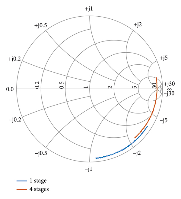
The S11 parameters of the n-stage rectifiers are shown in Figure 4, before matching, from 700 MHz to 1.1 GHz, to emphasize the high capacitance present on the circuit’s input.
The S 11 parameters of the 1-stage and 4-stage rectifiers, from 700 MHz to 1.1 GHz, without a matching network, using Z 0 = 50 Ω.
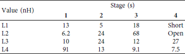
The matching networks are configured with an inductor-based, double “L” network topology, Figure 5.
The “double-L” matching network topology used to adapt the rectifiers.

The values for 50 Ω matching were simulated using ADS, and further adjustments were done in situ through an iterative, dichotomous approach. The values determined for the rectifiers are presented in Table 1.
This ensures an input return loss below −10 dB over more than 30 MHz of bandwidth at 935 MHz at lower power levels (−20 to −35 dBm), Figure 6.
The S 11 parameters of the 1-stage (a) and 4-stage (b) rectifiers, from 870 MHz to 970 MHz, matched, using Z 0 = 50 Ω, for varying input power levels.
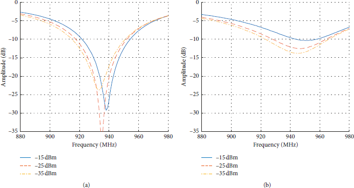
Due to varying diode capacitance as a function of power input P IN, the center frequency of the matched rectifiers tends to shift, though not significantly.
As illustrated in Figure 5, the centered frequency of the input return loss shifts with the input power, due to the dependence of the diode capacitance on the latter. This variation remains negligible regarding the achievable bandwidth over the considered range of power and targeted application. Indeed, for low-power IoT, the broadcasted data is sent at low bitrates, requiring narrow bandwidth, and powering methods via RF often use Continuous Wave (CW) carriers [Reference Nicot and Taris20].
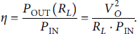
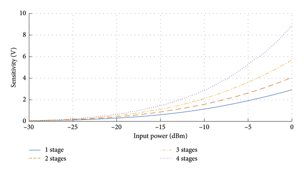
Rectifier performance is evaluated by two metrics: the sensitivity, S (1), which is the unloaded voltage output, and the efficiency, ƞ (2), which is the ratio of the output DC power (P OUT) to the input power (P IN), depending on the load R L :

Increasing the number of stages improves the sensitivity at low levels of power, Figure 7, but degrades the rectifiers’ efficiency accordingly, Figures 7(a) and 7(b). Interestingly, the increase of cascaded stages makes the efficiency increasingly independent of the load value R L , Figure 8. Similar work has yielded the same conclusions [Reference Kotani, Inoue, Komiyama, Chonan and Yamaguchi21]. Based on this analysis, we will use 4 stages to receive data and only one stage to harvest RF energy. Four stages were chosen for data reception in order to permit the node to receive data at a sufficient distance (up to 20 meters), while avoiding overloading the node’s reception module, as the sensitivity (and therefore outputted voltage) increases with the number of stages.
Measured rectification sensitivity S versus input power P IN, for power levels ranging from −30 dBm to 0 dBm.
Measured rectification efficiency ƞ versus input power P IN and load. (a) The efficiency ƞ for the 1-stage rectifier. (b) The efficiency ƞ for the 4-stage rectifier.

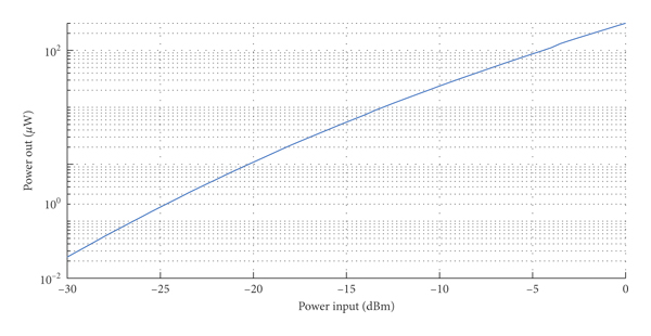
Figure 9 shows the amount of available output DC power, P OUT, of a 1-stage rectifier, as a function of the input power, PIN, with an optimal load applied for all power levels. Available power ranges from approximatively 200 nW at −30 dBm up to 450 μW at 0 dBm. To deliver 1 μW, a single stage rectifier requires an input power level of −21 dBm.
Measured power output P OUT versus input power P IN, for the 1-stage rectifier, for input power levels ranging from −30 dBm to 0 dBm.
2.2. Solar Panels
Solar energy is used as an alternative source of energy to complement RF harvesting when it is possible. Solar harvesting significantly increases the amount of energy available, enabling the use of an RF transmitter to provide data back to the requester.
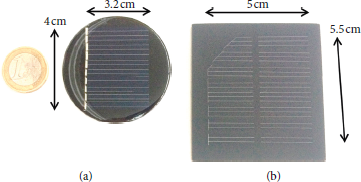
Two solar panels, a small one with circle shape and a large one with square shape, have been considered for the system, Figures 10(a) and 10(b), respectively. The operational areas of these panels are, respectively, 13.9 cm2 and 30.5 cm2. The open voltage, Figure 11, and available out DC power, Figure 12, of the solar panels are characterized in a controlled environment using white and yellow LEDs as illumination sources, in order to simulate realistic illumination conditions for the scenarios of application.
The solar panels with a 1-euro coin for reference. (a) The small solar panel. (b) The large solar panel.
Measured open voltage of the two solar panels, depending on both the luminosity available and the type of LED lighting.

Measured power output, P OUT, of the two solar panels, depending on both the luminosity available and the type of LED lighting, with illustrations of different luminosity levels, L.

The unloaded maximum voltage (open voltage) and maximum DC output power (available power) under full sunlight (L > 2000 lux) are 3.5 V and 1 mW for the small panel and 4 V and 2.5 mW for the square panel. In an indoor environment featuring windows (600 < L < 1500 lux), the open voltage ranges from 2.8 V to more than 3 V, and the power is between 500 μW and 1.5 mW for the square panel and between 250 μW and 600 μW for the small panel. In an office with only artificial light (L < 500 lux), the square panel still yields more than 50 μW and has an open voltage of more than 2 V. Yellow LEDs provide a larger open voltage and a higher output power, as they are more spectrally rich than white LEDs [Reference Tolnai and Rácz22]; however, the difference is not significant. Typical illumination levels were sourced from [23].
2.3. Power Management
2.3.1. Rectifiers
Rectification efficiency is dependent on load, and therefore it is not appropriate to directly supply digital circuitry, which may have different power consumption profiles, when the rectifier operates. This issue is remedied through the use of Maximum Power Point Tracking (MPPT), which loads the rectifier appropriately, permitting an extraction of the most amount of power possible at any given time [Reference Esram and Chapman24]. With the use of a boost converter, MPPT can be used to store energy into a ceramic capacitor-based storage element, thus providing adequate power when required. Ceramic-based capacitors are used for rectifier energy harvesting, due to their extremely low leakage profile, in consideration of the amount of energy that can be harvested from RF energy sources [Reference Lee, Lee, Schunke and Burton25].
A bq25570 power harvesting IC was chosen for this purpose, as it provides MPPT, a boost converter, and a buck converter with a variable output voltage and has a low quiescent current. Figure 13 shows the general operation and wiring diagram used for this work with the bq25570.
Schematic describing the bq25570 as used in this work, used for RF power harvesting and voltage regulation for the load (adapted from [10]).

The bq25570 has several different modes of operation. If the main storage element (C BIGSTOR) is depleted, it needs to be charged to a certain threshold (V CHGEN) before operation of the MPPT and the boost converter, through the use of a “cold-start” charge pump, with low efficiency (approximatively 5%). The storage element is then charged to an acceptable voltage level, in order to allow the main parts of the IC to operate. In order to avoid rapidly regressing into a cold-start state (especially due to the activation of the load), once the desired voltage is reached, a storage element threshold indicator (with hysteresis), V BATOK, is provided by the IC. It is used in this work in order to turn on or off the supply to the digital section of the node if power is scarce. The minimum storage voltage required to power on the system is 2.5 V, and the hysteresis shutoff is defined at 2.2 V. The values of the resistors to program the device are chosen using [Reference Ramadash26].
Although V CHGEN is approximatively 1.7 V, the values for the hysteresis circuit were programmed higher, to take into account the possibility of the absence of power and to insert a security margin to avoid regression into a “cold-start” state. The minimum storage voltage required to power on the system was set at 2.5 V, and the hysteresis shutoff set at 2.2 V. Although, theoretically, these values could both be equal to V CHGEN to ensure maximum energy usage if power should become unavailable, the limits were chosen to be higher than the former in order to avoid a regression into a cold-start state should there be an interruption in the RF energy source, in order to preserve an entry point into the high efficiency boost mode, when power is restored.
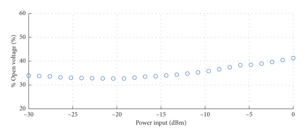
In order to perform MPPT, the bq25570 periodically samples the sensitivity, S, of the 1-stage rectifier through the R OC1/R OC2 divider bridge and applies a load according to the voltage present between R OC1 and R OC2 (S MPPT). The measured efficiency, reported in Figure 7, depending on the optimal loads from −30 dBm to 0 dBm, was determined for MPPT. From these loads, the optimum voltage levels that should be delivered to the bq25570 through the voltage divider are calculated. This is presented as the ratio of S MPPT/S in Figure 14. It can be seen that a value of around 35% presents optimal power transfer, especially at lower input power; therefore, R OC1 and R OC2 were set accordingly.
Optimum MPPT calculation, in order to size R OC1 and R OC2 to extract maximum power from the 1-stage rectifier.
2.3.2. Solar Panels
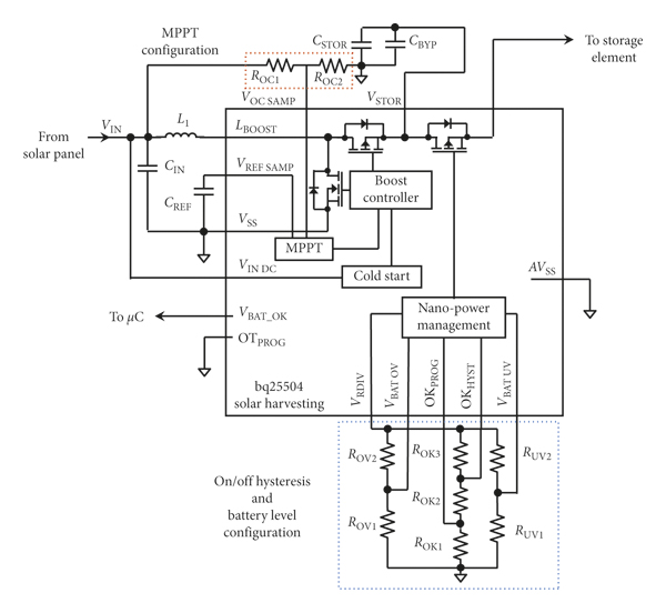
Similarly to rectifiers, solar panels also require the use of MPPT in order for the maximum available power to be extracted from them. For this purpose, a bq25504 power harvesting IC was used. It is similar to the bq25570, with the exception that it does not have an integrated buck converter and therefore cannot provide a regulated output voltage to a load. Figure 15 shows the general operation and wiring diagram used for this work with the bq25504. The storage element chosen for solar power harvesting is a 470 mF supercapacitor, which can store considerably larger amounts of energy than ceramic-based capacitors. However, these elements do have a higher leakage current [13, Reference Weddell, Merrett, Kazmierski and Al-Hashimi27].
Schematic describing the bq25504 as used in this work, used for solar power harvesting (adapted from [11]).
In order to combine both RF and solar energy together, a BAT17-04 Schottky diode [28] was introduced between the supercapacitor serving as a storage element for the bq25504 and the ceramic capacitor array serving as a storage element for the bq25570.
The use of a Schottky diode permits a completely passive solution permitting energy to be transferred from the solar energy circuit to the RF energy circuit, while avoiding a significant reverse drain of energy from the RF energy circuit if no solar power is available. The low threshold voltage of this diode also makes it possible to avoid significant energy loss during energy transfer. Similar techniques have been used in other work with combined RF/solar harvesters [Reference Niotaki, Giuppi, Georgiadis and Collado29, Reference Bito, Bahr, Hester, Nauroze, Georgiadis and Tentzeris30].
The same voltage thresholds and hysteresis values were used as in the previous subsection. Likewise, the MPPT ratio S MPPT/S can also be inferred from measured data, Figure 16. It can be seen that a value of around 70% presents optimal power transfer, with a variation of around plus or minus 5%, depending on the luminosity and solar panel type.
Optimum MPPT calculation, in order to size R OC1 and R OC2 for the extraction of maximum power from the solar panels.

2.4. Energy Storage
2.4.1. Rectifiers
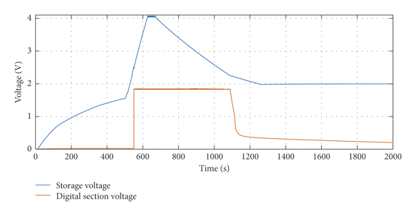
The bq25570 has two main modes of charging operation: “cold-start” (CS) mode, where a charge pump with low efficiency charges up the main storage element to about 1.7 V (VCHGEN), and a “warm-start” (WS) mode, where the MPPT and boost converter are active and charge the main storage element up to a configured voltage (4.0 V) [10]. The combination of both the CS and WS modes has been defined as “full-start” (FS) mode.
CS mode requires a minimum of 15 μW to be able to charge the storage element to VCHGEN, leakages notwithstanding. From Figure 9, it can be determined that a minimum RF power input of −13.1 dBm is required to bootstrap the system if the main RF energy storage element is empty. A typical charge and discharge curve of the system during normal operation was measured, Figure 17, without active communications. The digital section of the node’s output is regulated to 1.8 V.
The CS phase of the bq25570 can be seen from 0 s to 500 s, and WS phase can be seen from 500 s to 620 s, with the output to the digital section of the node turning on at 550 s, when the storage element reaches 2.5 V. Discharge can be seen from 650 s to about 1300 s, during which the bq25570 provides power to the digital section of the node until reaching the shutoff voltage of 2.2 V.
The amount of time taken to fully charge the system from an empty ceramic capacitor storage element of 470 μF was measured as a function of RF power input in Figure 18. No communications were active during this time.
bq25570 charge and discharge cycle, with a 470 μF ceramic capacitor storage element, and P IN = −10 dBm during charging.
Charge times in CS and WS modes increased quasi-linearly with the size of the ceramic capacitor storage elements. Discharge times were also measured and determined to be 425 s, 971 s, 1810 s, and 3505 s, respectively, for the 470 μF, 940 μF, 1860 μF, and 3720 μF ceramic capacitor-based storage elements.
The quasi-linearity of the charge and discharge times is logical, as the device is operating at a constant power discharge. This is because, during sleep mode, the node exhibits static, unvarying power consumption, and the bq25570’s quiescent current varies little with voltage, so charge and discharge times will tend to obey:

where t is the amount of time taken to discharge capacitor C BIGSTOR, between the initial and final voltages V INIT and V FINAL, respectively. P CONSUMPTION is the power consumption that is applied to the capacitor.
2.4.2. Solar Panels
The bq25504 also has two modes of operation, the CS and WS modes, similarly to the bq25570. Like the bq25504, CS mode on the bq25570 requires at least 15 μW to be able to charge the storage element in CS mode. However, when using a supercapacitor, the leakage current cannot be neglected [Reference Weddell, Merrett, Kazmierski and Al-Hashimi27].
The initial but worst-case leakage current of such devices can be as high as 100 μA (whether charged or discharged), and therefore the CS requires approximatively 20 μW of power in order to be able to charge the bq25504 to WS mode [11]. The leakage current, though initially high, eventually stabilizes to less than 1 μA after several days. This can be observed through the rate at which the voltage drops, Figure 19.
Time taken for the bq25570 to accomplish cold, warm, and full start using RF energy only, as a function of input power.

This exhibits the worst-case scenario of self-discharge, as it was charged instantly, using a standard power supply for approximatively 5 minutes. It should be noted that this leakage current does diminish after several days down to about 1 μA to 2 μA, due to the charging characteristics of such devices [Reference Weddell, Merrett, Kazmierski and Al-Hashimi27].
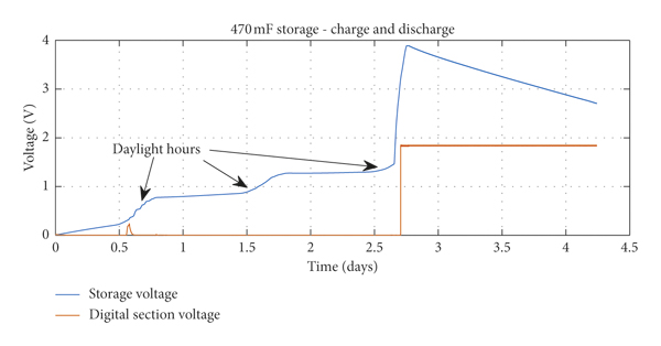
A charge and discharge cycle of the supercapacitor through solar energy was measured over a period of 100 hours, Figure 20, using the large solar panel, where the environmental luminosity varied between 100 lux during nighttime hours and 1000 lux during daylight hours.
Self-discharge curve of the 470 mF supercapacitor over several days, showing the voltage present.

It can be seen that the initial charge time in CS mode is very slow, due to the inefficiency of the charge pump in the power management IC, but is still possible, even if only 100 lux is permanently present. Once the WS mode is active, the charging of the supercapacitor becomes significantly faster, due to the activation of MPPT, which has a much higher efficiency (measured at least 70%). From Figure 20, it can be noted that, as long as there is enough luminous energy to charge the capacitor to at least its previous voltage before the next luminous cycle (i.e., work hours or daytime), the operation of the node may be maintained indefinitely in warm-start mode, which can permit the use of the node in low-luminosity environments due to the increased efficiency of WS mode.
Measurements indicate that the minimum amount of luminosity required to keep the node functional without discharge is 70 lux, after the supercapacitor was charged for several days, minimizing the leakage current, assuming no communications were present.
2.5. Communications
2.5.1. Node Reception
As this system is designed to consume as little power as possible, the use of a standard RF receiver is not feasible due to the high-power consumption of such devices which requires at least a couple of mW to operate [Reference Wang, O’Donnell, Ribetto, O’Flynn, Hayes and O’Mathuna31]. Therefore, the node is always in deep sleep mode when not being solicited, and reception (RX) communications are first processed using a 4-stage rectifier circuit to perform the envelop detection of an incoming OOK, or ASK, modulated RF signal at 935 MHz.
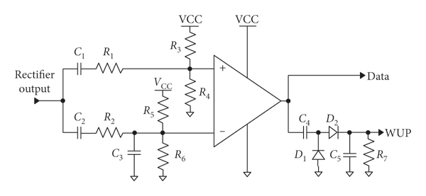
The wake-up radio demodulator circuit is presented in Figure 21. It provides a good trade-off between robustness and low-power consumption to demodulate data while minimizing false wakeups. Indeed, amplitude modulation schemes are prone to large and abrupt variations of the dynamic signal due the environment of propagation, which contribute to corruption of the demodulation process.
bq25504 charge and discharge cycle, with a 470 mF supercapacitor storage element, with the luminosity varying between 100 lux and 1000 lux.
The main component used for data demodulation is a TS881 comparator, chosen for its low quiescent current. V IN is the output of the 4-stage rectifier. R 2 and C 3 form a data slicer (low pass filter), which is used to demodulate incoming Manchester-encoded data. The RC time constant was chosen to be 5 times the baud rate in order to provide sufficient settling time while remaining adaptable to varying power levels.
C 1 and C 2, associated with R 1/R 3/R 4 and R 2/R 5/R 6, respectively, form high-pass filters in order to avoid false data detection which may arise from slow power level variations. The “+” and “−” input nodes of the comparator are polarized to half the supply voltage through R 3/R 4 and R 5/R 6, thus ensuring proper operation of the comparator. More specifically, the “+” node is slightly biased below the “−” node to avoid chattering, at the cost of decreased sensitivity.
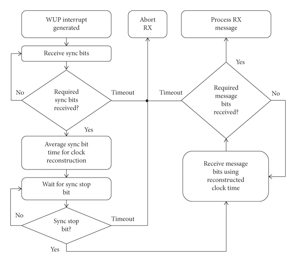
In the case of ASK modulation, data is sent along with power, whereas OOK modulation implies that the system is not powered during communications. RX communications are done at a speed of 800 bauds, but the algorithm in the microcontroller can be adapted to run from 40 bauds to 25.6 kilobauds.
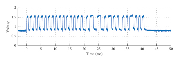
The frame format of messages sent to the node was implemented using Manchester encoding, with a synchronization preamble, Figure 22. This form of encoding provides several advantages. First, the synchronization preamble can be used to lock onto the baud rate with a certain error tolerance (clock reconstruction). Furthermore, it avoids long sequences of binary zeroes and ones which can induce demodulation errors in the data slicer. It does, however, increase the spectrum usage for an equivalent number of sent bits.
Comparator circuit for data reception; wake-up signal generation.
The synchronization subframe length, s, was chosen to be 16 bits, in order to allow for proper wake-up generation and baud rate detection. The actual message subframe length, n, is two bytes long (m = 16 bits). The first byte of the message subframe is the address of the node, which permits an addressing of up to 256 nodes, and the second byte is a command, subdivided into two nibbles. The first nibble indicates the operation, and the second contains an optional argument for the microcontroller to process. The frame is therefore 33 bits long.
The frame format for the node’s low-power wake-up radio, used in RX communications.

The RF signal is first rectified by the 4-stage rectifier, Figure 23, where it is then available for processing by the comparator and wake-up circuit. The wake-up detector has been adapted from [Reference Marinkovic and Popovici32].
Data frame sent to node, after rectification.
It is designed to allow data rates above a certain frequency to activate the wake-up circuit, which makes it robust against low-frequency, brutal changes in power levels or against external interference from other communications in the same band, which may be interpreted by the comparator as data.
The output of the comparator is a normalized representation of received binary data to V CC (1.8 V). This is used in two ways: to generate a wake-up signal with C 4, D 1, D 2, C 5, and R 7 (WUP) and also give data to the microcontroller (DATA) to be processed when the wake-up signal is generated, Figure 24.
Data frame normalization to 1.8 V and wake-up signal generation for the microcontroller.

The sensitivity of the circuit was measured, and the node messages could still be properly processed by the microcontroller with power input down to −31 dBm at the input of the 4-stage rectifier circuit.
2.5.2. Node Transmission
Transmission (TX) communications from the node are done using a low-power radio transmitter IC, the SPIRIT1. This IC is capable of sending data with diverse modulation formats, including OOK, ASK, FSK, and GFSK. Power levels used to transmit the data can be configured from 11 dBm down to −30 dBm. The baud rate of data transmission can also be configured from 1 kbps up to 500 kbps.
It can use either direct modulation or a standardized packet format. Using the standardized packet format, data transmission integrity can be verified using a Cyclic Redundancy Check (CRC). The Advanced Encryption Standard (AES) can also be used in order to secure data transmission. The module also includes a Carrier Sense Multiple Access (CSMA) algorithm, which can be exploited to detect if another module or device is already transmitting, thus avoiding packet collisions [17].
For the purposes of this work, 2-GFSK modulation was selected in order to transmit data, at a rate of 38.4 kbps, and the basic packet format was used in order to minimize overhead on the microcontroller. The frequency at which the data was emitted is 868 MHz. The frequency deviation for the modulation is 19 kHz. The output power level chosen for data transmission is −30 dBm. A transmission of the basic packet was collected via SDR and demodulated in order to show the digital data sent, using the default settings of the transmitter, Figure 25.
Standard “basic” data frame from the low-power TX module.

The packet is split into 4 main parts: the preamble, which is 64 bits long; the sync word, which is 32 bits long; the message, which is 3 bytes (or 24 bits) long; and the CRC checksum, which is 1 byte (or 8 bits) long. The packet format can be modified through registers present in the module, and additional fields can be added, depending on the usage scenario, which includes addressing capabilities, multipacket, or variable-length messages [17]. The demodulation of the received packets is performed on the same device transmitting data to the node. The supplied software is used to receive data packets. An example of packet reception, containing temperature data as the third byte, is shown in Figure 26.
Reception of data from the node. The third byte is ambient temperature as measured by the microcontroller, in hexadecimal format, between 25°C and 27°C in this case. The first two bytes are “T?” in ASCII.

2.6. Functionality
In order to use harvested energy and to manage the concurrent operation of different modules, the data demodulation capabilities and intelligent functions of this sensor node are provided by a PIC16LF1559 microcontroller, with an integrated temperature sensor [14]. Storage capabilities are implemented with an FRAM IC, using the SPI bus [15].
The PIC spends most of its time in sleeping mode and only wakes up when an event is received from the comparator/data slicer module. The Manchester decoding algorithm is implemented in a purely software-based manner, using interrupts and timer loops. The algorithm can be adapted for different synchronization formats, message sizes, and data transmission speeds and is presented in Figure 27. Once a message is received, it is then processed and, if successful, an action is performed, as illustrated in Figure 28.
Software algorithm used in order to decode the Manchester-encoded message received by the node.
Software algorithm used after reception of a correct message, showing a sample of available commands.
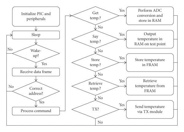
Table 2 presents a brief overview of currently implemented commands that can be sent to the node with the basic, 2-byte frame format. The PIC only processes these commands if the first byte of the frame matches its programmed address.

1 These commands are used for debugging purposes.
2 For these commands, n is a variable, ranging from 0 × 0 to 0 × F.
2.7. Assembled System
The different modules featured in the node were independently manufactured on 2- or 4-layer FR-4 substrate and soldered. The node, Figure 29, is further enhanced by using modular signal connectors.
The whole system, with all modules present. A 1-euro coin is provided for reference.
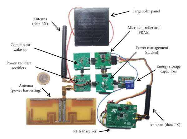
This modular, multiboard approach allows the experimentation with various assemblies of different subcircuit generations, in order to evaluate their performance independently. The presence of connectors also facilitates easy determination of power consumption by inserting measurement devices between the pins and permits easy debugging of various modules with measurement instrumentation.
3. Power Consumption Analysis
The estimated power consumption of the overall system is necessary in order to determine the viability of applicative scenarios of usage of the node. Indeed, it may be necessary to limit certain power consuming features of the node (notably the broadcasting of measured data) when limited power is available. Typically, when RF harvesting is the only source of energy, the system must operate in a restricted mode from a power consumption perspective.
This section fully characterizes the power consumption of the different modules of the node, depending on their phase of operation. The modules are categorized as digital and analog modules, as digital modules have more phases of operation than analog modules, with the latter having more predictable and static power consumption over time. VCC is the voltage delivered to the digital subsection and is configured at 1.8 V. A simulator that is constructed from measured data is then presented.
3.1. Analog Modules
3.1.1. Comparator
The comparator/wake-up module is the device that consumes the most power in sleep. This is primarily for two reasons. Firstly, in order to polarize the inputs of the comparator to
 , after the high-pass filter, Figure 20, the resistor network uses approximatively 180 nA, or 324 nW. Secondly, the comparator itself uses 220 nA, or 396 nW. Additional current used, when the WUP and DATA pins change due to the reception of data, was measured to be about 10 nA to 20 nA at most, or 18–36 nW. The module therefore consumes, at most, about 850 nW of power, continuously.
3.1.2. Power Management ICs
The bq25504 and bq25570 must also be considered when doing a power consumption analysis. During CS mode, the necessary minimum amount of power required to start up both devices is 15 μW, below which the device will never manage to enter WS mode, due to the inefficiency of the charge pump, which is approximatively 5%.
Once in WS mode, the power consumption of the devices varies relatively little, and it was measured, with no power on the input, to be around 500 nA, independently of voltage present on the storage elements. Depending on storage element voltage, this can range from a power consumption of 2 μW down to 850 nW. The efficiency of the buck converter, Figure 30, is measured with the storage element fully charged, using the methodology provided in its datasheet [10].
Efficiency of the buck converter of the bq25570, as a function of output current.
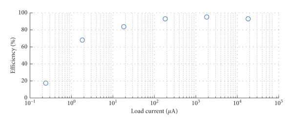
Buck converter efficiency exceeded 80% for load currents above 10 μA. However, for currents between 1 μA and 10 μA, efficiency dropped down to 60%, and for load currents below 1 μA, the efficiency is approximatively 20% or less.
3.2. Digital Modules
3.2.1. FRAM
The FRAM IC has several modes of operation: read mode, write mode, sleep mode, and idle mode. In sleep mode, current consumption is measured at 30 nA, or about 55 nW. During this mode, the FRAM is not available to process commands and must be woken up into idle mode in order to function. Wake-up time is measured to be 15 μs. During idle mode, the FRAM module consumes 4 μA of current or 7.2 μW. In this mode, the FRAM module is ready to accept read and write commands. Reading data from one address consumes 2.13 mA, or 3.83 mW of energy. Writing data consumes 2.32 mA, or 4.17 μW of energy. The power consumption of FRAM modules is significantly lower than flash devices [Reference Medu33].
3.2.2. Microcontroller
The PIC microcontroller, similarly to the FRAM, has several modes of operation: sleep mode, message receiving mode (which can be further separated into false wakeups and full messages), data processing mode (which includes SPI transactions), and ADC measurement mode.
The power consumption in sleep mode is measured to be 40 nA or 72 nW. In message receiving mode, whether due to false wakeups or actual messages, the consumption of the microcontroller is the same, at 230 μA, or 415 μW, though the time spent processing these different modes is different. In data processing mode, the power consumption is 410 μA, or 738 μW, and, finally, in temperature measurement mode, the power consumption is 800 μA, or 1.44 mW.
Another metric that is of importance is the consumed energy per bit received. As the microcontroller receives messages at 800 bauds and consumes 415 μW while receiving a message for 40 ms, it consumes 16.6 μJ to receive 33 bits (a message of 16 bits and a synchronization subframe of 17 bits), which is approximatively 503 nJ per bit received.
3.2.3. TX Module
The data TX module must be operated in a particular order so as to ensure data transmission. It must be turned on, reset, and then set into its ready operating state. Afterwards, the Voltage Controlled Oscillator (VCO) operating within the integrated PLL must be calibrated, after which it must also be returned to a ready operating state. After this initialization phase, data may be sent to the transmitter buffer, and the device may send data. At the end of the transmission, it returns into ready state and may then be shut down.
The device in shutdown mode consumes 2 nA of current, or 2.6 nW. In ready mode, it consumes 430 μA, or 774 μW. When calibrating its VCO, it consumes 6.72 mA, or 12.33 μW. Finally, when transmitting data, it consumes 9.58 mA, or 17.56 mW.
As the module sends messages at 38.4 kbps and consumes 17.56 mW while sending a message for 3.75 ms, it consumes approximatively 65.9 μJ to transmit 128 bits, which is 514 nJ per bit sent during the actual transmission state. If VCO calibration and module setup are to be included, then the power consumption per bit increases to 592 nJ per bit.
3.3. Module Power Consumption
The modules comprising the node are split into two categories: analog modules and digital modules. Analog modules generally present an invariant power consumption rate whatever the node’s operating state is, though the warm- and cold-start modes of the power management ICs are exceptions.
Table 3 presents an overview of the power consumption of the analog modules. The power consumption of the power management ICs is variable, as they are supplied by the storage elements, whose voltage may vary from 1.8 V to 4 V in warm-start mode.

Table 4 presents an overview of the power consumption of the digital modules, depending on their different states of operation. As they are supplied by the power management modules with a constant voltage of 1.8 V, their consumption only varies depending on the state of operation.

3.4. Node Operation
Excluding the inefficiencies and quiescent current consumption of the power management modules, the static consumption of the node in sleep mode is defined as the sum of the comparator, FRAM, microcontroller, and transceiver power consumption in sleep mode.
All other power consumption states are a combination of the modules’ operating states as shown in Tables 3 and 4, whose operation is organized by the microcontroller as fast as possible, in order to minimize power consumption. The average power consumption of the node while performing select commands was measured and is presented in Table 5.

Static power consumption of the node is 920 nW, or less than a microwatt. Most messages have similar power consumption profiles, around 17 μJ per message, including any operation which uses the different modules on the node, due to the speed at which the operations are conducted.
There are, however, two exceptions to this generalization. The first one is when the node receives a false wakeup. Most received messages are interfering signals, which are not OOK/ASK modulated, or use an incompatible frame format. With this in mind, the message reception code was designed to time-out after approximatively 16.8 ms if an incorrect message is received.
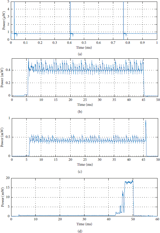
The second exception is when the node is asked to transmit data, as this is a time and energy consuming operation, during which the node consumes about 97.8 μJ of energy. When transmitting, however, other operations, the node performance has negligible power consumption in comparison to sending data, Figure 31.
Power consumption of the node for different commands. (a) The power consumption when the node is idle. (b) The power consumption when a message is received. (c) The power consumption when the FRAM is solicited for a read or write operation. (d) The power consumption when a data TX command is issued.
3.5. Simulator
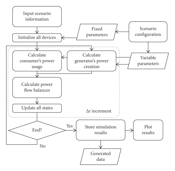
The power consumption simulator is derived from power consumption data measured in situ. The simulator uses an iterative approach to determine power consumption over a small time interval, Δt. Once the calculation of the power consumption during Δt is complete for all elements, the states of operation of each device are updated. The general equation modeling the consumption of any given module of the node in the simulator is shown below:

where P is the power consumption, or generation of any module in the node, M is the change in power consumption over the previous Δt time increment, and S is the current state of operation of the node. This includes any changes in solar and RF levels, power storage element levels, and any operations undertaken by the node that may modify the power consumption of the node. The changes in power consumption are then summed or subtracted, depending on whether the device is a power consumer or generator, in a chain that corresponds to power flow.
An overview of the simulated algorithm is presented in Figure 32:
Overview of the simulator algorithm.
4. Scenarios of Operation
Several applicative scenarios were envisioned for this type of device. Scenarios have been classified according to the type of power mainly used to power the node, being that of RF energy or of solar energy. Using data derived from part III of this work, simulation of expected results was theoretically calculated. Measured data is also presented and compared to theoretical predictions.
Theoretical predictions of power consumption were estimated by taking into account the leakage current of storage devices, the power consumption of the power management modules, and their inefficiencies, especially in regard to the low performance of the bq25570’s buck converter. These values were integrated into a program capable of simulating the power consumption of the node over time, in order to determine the accuracy of the simulations in regard to the actual power consumption.
For these scenarios, a data measurement operation shall be defined as the combination of a temperature measurement command with an FRAM write command. A data transmission operation shall be defined as an FRAM read command combined with a data transmission command.
It should be noted that the maximum speed at which the node can receive commands is approximatively at 6.67 Hz, or 150 ms. Although the microcontroller takes approximatively 50 to 60 ms to fully process a command (Figure 30), the wake-up radio takes approximatively 150 ms to return to a “known state,” wherein the wake-up generation circuit is fully discharged (Figures 20 and 23), thereby limiting the speed to a maximum of 6.67 requests per second.
4.1. Continuous RF Operation
Continuous RF operation of the sensor node means that it will be constantly powered, but only through RF energy, from a 28 dBm emitter, with a 3 dBi patch antenna, operating at 935 MHz. The ceramic capacitor storage elements recharge back up to 4 V if powered with at least −15.1 dBm of power input, which is the minimum amount of power required to keep the PIC, comparator, and bq25570 operational (while sleeping and without communications). This corresponds to a power usage of 7 μW, of which the bq25504 uses 2 μW. The high usage of the digital subsection can be explained by the low efficiency of the buck converter for very small supply currents (Figure 30). The bq25504 will be considered to be nonoperational in this mode and therefore will not consume any energy. The storage element for this scenario is a 3720 μF ceramic capacitor-based element.
The main criterion to evaluate the performance of continuous operation of the node is how fast measurements can be performed (maximum measurement speed) without the main storage capacitor discharging, which will depend on the power input to the rectifier.
This scenario will be played out in two parts: for the first part, the node will operate in RX-only mode, where the only instructions it will receive are that of data measurement and storage; during the second part, in addition to RX mode, it will also operate in TX mode.
4.1.1. RX-Only Operation
The calculated and measured speeds at selected points of this metric are reported in Figure 33.
Maximum measurement speed as a function of input power, with a 3720 μF ceramic capacitor-based storage element, for data measurement operations.

At measurement intervals of 10, 50, 100, 500, and 1000 seconds, the node requires, respectively, −6.2, −11.3, −12.5, −14.2, and −14.5 dBm of input power in order to remain operational.
It can be seen that as the frequency of measurements becomes increasingly close to the theoretical 6.66 Hz maximum possible, the amount of power required for maintaining the system operational increases rapidly. It is not possible to reach the theoretical limit of 6.66 Hz, as this would require more instantaneous energy than the rectifier can provide, 10 mW, if it is supposed that a maximum input power of 0 dBm is available for this scenario. As the interval between measurements increases, the power level trends towards the hard limit of −15.1 dBm.
The higher levels of power required as the frequency of measurements increases are likely due to cumulated interaction of inefficiencies (buck converter, MPPT out of range as power input levels increase,…) in the node as power consumption rises.
The typical distance at which the node can operate in RX-only continuous RF mode ranges from 1 m to 6 m, though the amount of time between measurements increases with distance, in order to give enough time for the storage element to recharge and return to its previous level. The recharge time for 1, 2, 5, and 6 m distances was measured to be 10, 21, 344, and 1505 s, respectively. Operation at 10 m was also observed as a result of multipath propagation in the measurement environment.
4.1.2. RX and TX Operation
Similarly to the first part of the scenario, the node will now be instructed to perform a data measurement and a data transmission operation. This will reduce the effective maximal frequency rate of measurements down to 3.33 Hz. The calculated and measured speeds at selected points of this metric are shown in Figure 34.
Maximum measurement speed as a function of input power, with a 3720 μF ceramic capacitor-based storage element, for data measurement and data transmission operations.

At measurement intervals of 10, 50, 100, 500, and 1000 seconds, the node requires, respectively, −1.9, −7.6, −9.7, −13.2, and −14 dBm of input power in order to remain operational.
The node is more restricted in terms of measurement speed, due to the power consumption of transmission operations, which are nearly an order of magnitude larger than reception and measurement only operations; however, operation is still possible with only RF power.
4.2. Fully Autonomous Operation
As autonomous operation would require at least autonomy of a day (or more); it is therefore necessary to use a supercapacitor to store the energy required to power the circuit during sleep mode.
In this second scenario, a 470 mF capacitor is charged to full capacity at 4 V, for 30 minutes, using a standard power supply, and hot-plugged into the bq25504 circuit. No power, whether solar or RF energy, was given to the device. Both the bq25570 and the bq25504 operated in WS mode during the length of the scenario.
The main criterion to evaluate the performance of this autonomous operation of the node is how long it could operate with main storage supercapacitor discharging, depending on the frequency of measurements.
Discharge time was measured to be 2.25 days with no measurements. This is considered to be the case scenario, as the energy drain is considered to be only supercapacitor self-discharge, in combination with the quiescent current of the node in sleep mode. The worst-case scenario, on the other hand, is when the PIC is nearly continuously solicited.
4.2.1. RX-Only Operation
The calculated and measured speeds at selected points of this metric are reported in Figure 35.
Maximum node autonomy is a function of command frequency, with a 470 mF supercapacitor storage element, for data measurement operations.

At measurement intervals of 1 s, 5 s, 10 s, 1 min, 1 hour, and 2.8 hours, the autonomy of the node is, respectively, 12, 29, 37, 49, 53, and 53 hours. This is close to, but slightly less efficient than, theoretically predicted results. As measurement intervals increase to more than one hour, the static power consumption of the system overtakes that of the power used during normal operations, and so the autonomy varies little.
As measurements increase in frequency, the autonomy of the node decreases, though with a measurement every ten seconds, the node still has autonomy of 37 hours. If the node is not solicited, the autonomy of the node is approximatively 54 hours. This is a hard limit which depends on the supercapacitor leakage and the power consumption of the whole node.
Using a larger supercapacitor, or higher maximum storage element voltages, would increase the autonomy of the node. However, larger storage elements would come at a cost of longer cold-start times.
For longer autonomy requirements, it may be necessary to implement a cold-start charge method that will rapidly kick-start the system into warm-start mode, which may use existing energy harvesting methods (i.e., leave the node under a very bright light or leave the node next to a high-power transmitter, until it indicates that it is operational) or require a cable-based solution.
4.2.2. RX and TX Operation
The calculated and measured speeds at selected points of this metric are reported in Figure 36.
Maximum node autonomy is a function of command frequency, with a 470 mF supercapacitor storage element, for data measurement and data transmission operations.

At measurement intervals of 1 s, 5 s, 10 s, 1 min, 1 hour, and 2.8 hours, the autonomy of the node is, respectively, 4, 13.5, 21, 41, 52, and 53 hours. The autonomy of the node has decreased compared to the previous subscenario, due to the high consumption of data transmission operations. However, at measurement intervals of over an hour, the node still presents similar autonomy.
4.3. Solar Operation
The autonomy and power consumption of the node have been characterized in autonomous mode. Solar energy is analyzed, using the large solar panel and both LED types.
As solar energy can easily provide sufficient energy to power the node, the main criterion for this scenario will analyze the amount of luminosity required in order to recharge the node during the day, supposing that it is solicited during the night. In regard to the duration of a day, a pessimistic case of 8 hours of light and 16 hours of darkness will be supposed. Furthermore, it will be supposed that the node will always be operating in warm-start mode.
Figure 37 shows the amount of time required for the node to charge from the beginning of warm-start mode until the storage element (supercapacitor) is full, as a function of luminosity, supposing that the node is not solicited.
Node warm-start charge time as a function of luminous intensity.

It can be observed from Figure 35 that, for the white LEDs, at least 155 lux is required to recharge the node in 8 hours and that, for the yellow LEDs, 135 lux is required. This supposes that the node is fully depleted in terms of the warm-start mode but has not yet entered cold-start mode.
In the context of this scenario, if the node is solicited at night, then 16 hours of autonomy is required. From Figures 35 and 36, it can be determined that the node must not be sent commands more than once every 1.5 seconds and every 7 seconds, respectively, for RX and TX/RX operation modes, in order to stay in warm-start mode. Therefore, it is possible to conclude that the node may operate in environments with luminosity as low as 150 to 200 lux for an indefinite amount of time, with reasonable environmental sensing capabilities.
5. Analysis
RF harvesting techniques can produce work which is capable of generating energy with low levels of power input, such as [Reference Piñuela, Mitcheson and Lucyszyn4], where charging of storage occurs with power levels of −29 dBm, without any load present. Other RF-only harvesting systems have produced similar performance with this work, such as [Reference Taris, Vigneras and Fadel19, Reference Kotani, Inoue, Komiyama, Chonan and Yamaguchi21, Reference Usami, Komiyama, Chonan, Yamaguchi and Kotani34], with power harvesting being usable, without load, with power input levels around −20 to −25 dBm. Distances at which the node could operate from a 28 dBm power source ranged from 1 m to 6 m.
Combining RF and solar energy leads to diverse performance depending on the architecture used, such as [Reference Niotaki, Giuppi, Georgiadis and Collado29, Reference Bito, Bahr, Hester, Nauroze, Georgiadis and Tentzeris30, Reference Sample, Braun, Parks and Smith35, Reference Bito, Hester and Tentzeris36]. Due to different topologies and solutions used, it is difficult to compare such work homogeneously; however, it can be noted that solar energy delivers more energy than RF harvesting and that the performance of this work was similar to [Reference Bito, Bahr, Hester, Nauroze, Georgiadis and Tentzeris30]. In regard to the previously developed node [Reference John, Thierry and Taris8], the minimal power requirements to power this improved node in sleep mode are quasi-identical, as the added elements have very little sleep current, in the range of several nA. The addition of a solar-powered energy source in this work extends the autonomy of the node in environment where solar energy, even at ambient levels, is available.
As sleep current is not negligible compared to the power consumption of storage element leakages and power management IC quiescent currents, it is normal that performance metrics are worse than power harvesting systems in which no load is present.
Integration of a single antenna with both data and power reception was attempted. However, the integration was not possible, due to interference generated by the boost converter used for RF power harvesting. Indeed, the constant modification of the load impedance presented to the rectifiers, in order to perform MPPT, caused interference in the data reception (comparator) circuit, creating a situation in which false wakeups were continuously generated.
Furthermore, this work adds data retransmission capabilities compared to the previously developed node [Reference John, Thierry and Taris8]. This is useful, as it makes measurement data retrieval possible without having to make any physical connections to the node.
A custom-based interface using SDR was also created for sending commands to the node. Furthermore, this work does not only analyze metrics of the power harvesting elements of IoT nodes but develops details on the more functional aspects of the node. This includes what the node can do, in terms of functionality, how it does this, and a list of the performance of different modules, in order to see where optimization is required in order to reduce power consumption.
These additions have also permitted the creation of more complex scenarios of operation for the node. Scenarios in the previous work [Reference John, Thierry and Taris8] were limited to the amount of measurement operations that could be done with a set RF power input, and the autonomy of the node was, at best, limited to several hours.
In this work, the node can now operate for several days without any power source present (under the assumption that its storage elements are full), and the varied power sources increase energy redundancy, should one of the sources of power be not available. A greater variety of scenarios of operation is also possible with the further addition of a data retransmission module.
A power consumption simulator, which was not present in our previous work [Reference John, Thierry and Taris8], is also developed based on measured performance data and is used to compare measured performance in real settings with theoretical performance. Theoretical predictions and real data match closely. Furthermore, the simulator can be used in order to create and test other hypothetical scenarios before they are implemented, which can be used to test their viability before requiring measurements to be undertaken.
There are several limitations in this system that could be improved upon. On rare occasions, false wakeups can also trigger the microcontroller, which will waste energy trying to process data. This is partly remedied by using a timeout counter in the software loop, to minimize time spent decoding erroneous/false messages. A different reception architecture or modulation scheme should be considered, as in [Reference Oh, Roberts and Wentzloff37]. More energy efficient transceivers could also be used [Reference Molnar, Lu, Lanzisera, Cook and Pister38].
Another limitation is that of the bq25570 and bq25504 power management ICs, which are being used near their lower limits in terms of energy input, and therefore they do not always provide highly efficient energy transfer, which can easily triple the static energy consumption in sleep mode or cause long cold-start charging times. This could be mitigated by using custom-designed power management ICs, as in [Reference Paing, Falkenstein, Zane and Popovic39], or by using extremely low-power techniques to create equivalent replacements [Reference Bito, Hester and Tentzeris36].
Future additions that could be explored for this work include adding a larger variety of environmental sensors, which remains possible using the SPI bus present on the microcontroller. Additionally, the use of other power harvesting methods (such as thermoelectric modules) should be considered in order to increase the diversity of powering methods, to improve redundancy in terms of power availability.
6. Conclusion and Perspectives
This work demonstrates the possibility of creating a COTS-based, hybrid RF, and solar-powered IoT sensor node, capable of environmental sensing with a restrained power budget. The active section of the node consumes 920 nW of power in sleep mode, of which 870 nW is used for the wake-up circuitry.
During RF-only power operation (in the 900 MHz ISM band), the device may function with power levels down to −15.1 dBm, albeit with a cold-start requirement of −13.1 dBm, with a 28 dBm transmitter capable of providing both data and energy.
In solar mode, the device may function with luminosity levels down to 70 lux, albeit with a cold-start requirement of 100 to 150 lux, depending on supercapacitor leakage current, which is a typical lighting situation in an office or a house.
The system is fully operational, able to handle both communications and RF energy transfer over the same band, and, charge time notwithstanding, operate over a period of one or two days with the presence of a supercapacitor as a storage element. Additionally, the node is capable of wirelessly transmitting back data when requested to do so.
This work characterizes various operational scenarios that IoT nodes could be used in, giving an additional insight into the abilities and limitations that are possible in a small subset of potential operating environments. Besides cartography of different modes of operation, at the system level, a model is proposed based on the analysis and characterization of the power consumption of the functions featured in the proposed hybrid node. The resulting implementation exhibits a good correlation with actual measurements, thus allowing for prediction of the node’s performance in various environments, or other hypothetical scenarios.
Data Availability
The data used to support the findings of this study are included within the article. Other data used to support the findings of this study are available from the corresponding author upon request.
Conflicts of Interest
The authors declare that there are no conflicts of interest regarding the publication of this paper.
Acknowledgments
The authors would like to thank M. De Matos for her help in using certain measurement instrumentation and Y. Faize for the loan of his Joulescope.


 Open access

