






1. Introduction
The well-known Maxwell’s equations
 \begin{equation}\begin{cases}\nabla \times \mathcal{H}=\mathcal{J}+\partial_t \mathcal{D} & \text {(Amp\grave{e}re's Circuital Law), } \\ \operatorname{div}(\mathcal{D})=\rho & \text {(Gauss' Electric Law), } \\\partial_t \mathcal{B}+\nabla \times \mathcal{E}=0 & \text {(Faraday's Law of Induction), } \\\operatorname{div}(\mathcal{B})=0 & \text {(Gauss' Magnetic Law) }\end{cases}\end{equation}
form the foundation of classical electromagnetism, classical optics, electric, and magnetic circuits, together with the Lorentz force law. Here,  $\mathcal{E},\,\mathcal{B},\,\mathcal{D},\,\mathcal{H},\,\mathcal{J}:\Omega\times\mathbb{R}\rightarrow\mathbb{R}^3$ correspond to the electric field, magnetic induction, electric displacement field, magnetic field intensity, and the electric current intensity, respectively, where
 $\Omega\subset\mathbb{R}^3$ is a smooth domain or
 $\Omega=\mathbb{R}^3$. It is worth noticing that these physical quantities are all time-dependent vector fields. Besides, ρ is a scalar field representing the electric charge density. In order to solve the field quantities, we also need the following constitutive relations
 \begin{equation}
\mathcal{D}=\varepsilon\mathcal{E}+\mathcal{P}_{\mathrm{NL}}\quad\text{and}\quad\mathcal{H}=\frac{1}{\mu}\mathcal{B}-\mathcal{M},
\end{equation}
where  $\mathcal{P}_{\mathrm{NL}}$ stands for the nonlinear polarization field and
 $\mathcal{M}$ stands for the magnetization field and
 $\varepsilon,\,\mu$ are the permittivity and the permeability respectively. Suppose there are no currents, charges, or magnetization, i.e.,
 $\mathcal{J}=0$,
 $\mathcal{M}=0$ and ρ = 0, by using the constitutive relations (see Saleh and Teich [Reference Saleh and Teich31]), Maxwell’s equations (1.1) lead to the following nonlinear wave equation
 \begin{equation}
-\partial_t^2 \mathcal{P}_{\mathrm{NL}}=\varepsilon(x) \partial_t^2 \mathcal{E}+\nabla \times(\mu(x)^{-1} \nabla \times \mathcal{E})
\end{equation}
for the electric field  $\mathcal{E}$. The electric field
 $\mathcal{E}$ is said to be time-harmonic (also monochromatic) with frequency ω if
 \begin{equation*}
\mathcal{E}(x, t)=u_1(x) \cos (\omega t)+u_2(x) \sin (\omega t) \quad \text {for } x \in \Omega \text\ \text{and }\ t \in \mathbb{R} .
\end{equation*}
With the development of nonlinear optics and the rise of laser technology, the nonlinear response of a medium to electromagnetic waves has appeared in many physical phenomena and many types of nonlinear polarization models, which have been built in [Reference Stuart35]. Without loss of generality, we first suppose that the nonlinear polarization is of the form ([Reference Bartsch and Mederski6])
 \begin{equation}
\begin{aligned}
\mathcal{P}_{\mathrm{NL}}(x,\mathcal{E})=\chi_1(&x,f_1(|\mathcal{E}|)) u_1(x) \cos (\omega t)+\chi_2(x,f_2(|\mathcal{E}|)) u_2(x) \sin (\omega t),
\end{aligned}
\end{equation}
where  $\chi_1, \chi_2$ are two scalar susceptibilities and
 $f_1,f_2$ characterizes the dependency relationship between
 $\chi_1,\chi_2$ and
 $\mathcal{E}$. Then, (1.3) reduces to the system
 \begin{equation}
\left\{\begin{array}{l}
\nabla \times\left(\mu(x)^{-1} \nabla \times u_1\right)-\omega^2 \varepsilon(x) u_1=\omega^2\chi_1(x,f_1(|\mathcal{E}|)) u_1 \text {in } \Omega, \\
\nabla \times\left(\mu(x)^{-1} \nabla \times u_2\right)-\omega^2 \varepsilon(x) u_2=\omega^2\chi_2(x,f_2(|\mathcal{E}|)) u_2 \text {in } \Omega .
\end{array}\right.
\end{equation}
Looking for the semi-trivial solution, where one of  $u_1, u_2$ is trivial or where
 $u_1=u_2$, one is led to the following semi-linear curl-curl problem
 \begin{equation}
\nabla\times(\nabla\times u)=f(x,u)
\end{equation}
in a smooth bounded domain or in  $\mathbb{R}^3$, which has been recently studied for example in [Reference Azzollini, Benci, D’Aprile and Fortunato2, Reference Bartsch and Mederski5, Reference Gaczkowski, Mederski and Schino17, Reference Mederski22, Reference Mederski23, Reference Mederski, Schino and Szulkin26, Reference Mederski and Szulkin27]. Generally speaking, (1.6) is much more challenging to deal with than the usual Schrödinger equation since the curl-curl operator
 $\nabla\times(\nabla\times\cdot)$ has infinite-dimensional kernel consisting of all the gradient vector fields. Therefore, we have to deal with the compactness issues caused by the infinite-dimensional kernel even if the nonlinearity f is sub-critical with respect to u. For a long while, the assumption that the growth of
 $f(x,u)$ with respect to u is sub-critical has been essential in finding a general solution (which means a solution without any predetermined symmetric property) of equation (1.6). Surprisingly, in 2021, Mederski and Szulkin first provided a remarkable study about the following critical curl-curl problem in
 $\mathbb{R}^3$
 \begin{equation}
\nabla\times(\nabla\times u)=|u|^4u,\quad u\in W_0^6(\operatorname{curl} ; \mathbb{R}^3).
\end{equation}
In [Reference Mederski and Szulkin27], Mederski and Szulkin proved that there exists a ground state solution of the scalar problem (1.7) by a new and delicate concentration-compactness analysis on the curl operator. They also performed an analysis on a Sobolev-type inequality for the curl operator, which possesses similar properties to the classic Sobolev inequality in  $\mathbb{R}^3$. Later in 2023, Gaczkowski, Mederski, and Schino [Reference Gaczkowski, Mederski and Schino17] studied the multiple solutions problem to (1.7). They proved that there exists a sequence of
 $\mathcal{SO}(2)\times \mathcal{SO}(2)$-symmetric solutions to (1.7) with blow-up energy. Moreover, they showed that the solutions to the problem (1.7) are in one-to-one correspondence with the solutions to a singular Schrödinger equation in
 $\mathbb{R}^3$. For more results on the multiple solutions to a sub-critical curl-curl problem, see [Reference Gaczkowski, Mederski and Schino17] for more details. We also refer the readers to [Reference Amrouche, Bernardi, Dauge and Girault1, Reference Bartsch and Ding3, Reference Bartsch, Dohnal, Plum and Reichel4, Reference Benci and Fortunato7, Reference Bieganowski8] [Reference Chen, Du and Zou11, Reference Hirsch and Reichel18, Reference Kirsch and Hettlich19, Reference Mandel21, Reference Mederski24, Reference Mederski, Schino and Szulkin26] [Reference Mederski and Schino25, Reference Picard, Weck and Witsch30, Reference Stuart34–Reference Stuart and Zhou37, Reference Zeng44] and the references therein for the abundant and excellent results on the time-harmonic Maxwell’s equations (1.6).
Mathematically, the assumption on (1.5) that one of  $u_1, u_2$ is trivial or
 $u_1=u_2$ is somehow oversimplified. Therefore, studying the non-trivial solutions of (1.5) is one of the author’s interests. However, the problem of system with curl operator is rarely studied in the past few decades. In 2023, Wen and Zhao [Reference Wen and Zhao41] studied the following sub-critical weakly coupled time-harmonic Maxwell’s equations
 \begin{equation}
\begin{cases} \nabla \times(\nabla \times u_1)-V_1(x)u_1=\mu_1|u_1|^{p-2}u_1+2\lambda\beta|u_1|^{\beta-2}|u_2|^\alpha u_1 & \text {in } \Omega, \\ \nabla \times(\nabla \times u_2)-V_2(x)u_2=\mu_2|u_2|^{p-2}u_2+2\lambda\beta|u_1|^\beta|u_2|^{\alpha-2}u_2 & \text {in } \Omega,\\
\nu\times u_1=\nu\times u_2=0, &\text{on }\partial\Omega,
\end{cases}
\end{equation}
where  $\Omega \subset \mathbb{R}^3$ is a smooth bounded domain with exterior normal
 $\nu: \partial \Omega \rightarrow \mathbb{R}^3$,
 $V_1, V_2: \Omega \rightarrow \mathbb{R}$ are two continuous functions which are positive, bounded away from 0, and less that the first Maxwell eigenvalue,
 $\mu_1, \mu_2$, and λ are positive constants,
 $2 \lt p \lt 6$,
 $\alpha, \beta \gt 1$, and
 $\alpha+\beta=p$. By improving and using the variational approach in [Reference Bartsch and Mederski5, Reference Szulkin and Weth38], they proved that there exists a ground state solution for system (1.8) if
 $\mu_1 \lt \eta$ or
 $\mu_2 \lt \eta$ for some constant
 $\eta=\eta(p)$. Besides, under these assumptions, they proved that (1.8) admits a sequence of non-trivial solutions whose energy tends to infinity. Moreover, if Ω is a cylindrically symmetric domain, then system (1.8) has infinite bound state solutions with cylindrical symmetry. Recently, together with Jingxuan Sun and Wenming Zou [Reference Song, Sun and Zou32], the author studied the following Lane–Emden system for curl-curl operator
 \begin{equation}
\begin{cases} \nabla \times(\nabla \times u_1)=|u_2|^{q-2}u_2 & \text {in } \Omega, \\ \nabla \times(\nabla \times u_2)=|u_1|^{p-2}u_1 & \text {in } \Omega,\\
\nu \times u_1=\nu \times u_2=0 & \text {on }\partial\Omega \end{cases}
\end{equation}
in a simply connected, bounded Lipschitz domain  $\Omega\subset\mathbb{R}^3$ with connected boundary. When Ω is convex or has
 $C^{1,1}$ smoothness boundary, and
 $p,q\in(2,6)$, they established the existence of a non-trivial ground state solution with positive energy and the existence of infinitely many non-trivial solutions. Besides, they found a lower bound estimate of the ground state energy level. Finally, they obtained a kind of symmetry theorem for the components u 1 and u 2 on the exponents p and q. Notice that in the above two papers, the sub-critical condition is necessary.
In this paper, we mainly study the following critically coupled time-harmonic Maxwell’s equations
 \begin{equation}
\begin{cases} \nabla \times(\nabla \times u_1)=\mu_1|u_1|^4u_1+\beta|u_1||u_2|^3u_1 & \text {in } \mathbb{R}^3, \\ \nabla \times(\nabla \times u_2)=\mu_2|u_2|^4u_2+\beta|u_1|^3|u_2|u_2 & \text {in } \mathbb{R}^3,\end{cases}
\end{equation}
where  $u_1,u_2:\mathbb{R}^3\to\mathbb{R}^3$. This system arises naturally as a counterpart of the equation (1.7). To the best of our knowledge, this paper is the first study on weakly coupled time-harmonic Maxwell’s equations with critical exponent.
To begin with, let us introduce some basic knowledge of the variational setting. Define
 \begin{equation*}
W^6(\operatorname{curl} ; \mathbb{R}^3):=\{u\in L^6(\mathbb{R}^3,\mathbb{R}^3):\,\nabla\times u\in L^2(\mathbb{R}^3,\mathbb{R}^3)\},
\end{equation*}
which is a Banach space if provided with the norm
 \begin{equation*}
\|u\|_{W^6(\operatorname{curl} ; \mathbb{R}^3)}:=\left(\|u\|_6^2+\|\nabla \times u\|_2^2\right)^{1 / 2} .
\end{equation*}
Here and in the sequel  $\|\cdot\|_p$ denotes the standard Lp-norm for
 $p \in[1, \infty]$. It is worth mentioning that the curl,
 $\nabla\times u$, has to be understood in the distributional sense. We also define
 \begin{equation*}
W_0^6(\operatorname{curl} ; \mathbb{R}^3):=\text {the closure of } {C}_0^{\infty}(\mathbb{R}^3, \mathbb{R}^3) \text \ \text{in } W^6(\operatorname{curl} ; \mathbb{R}^3) .
\end{equation*}
Notice that  $W_0^6(\operatorname{curl} ; \mathbb{R}^3)=W^6(\operatorname{curl} ; \mathbb{R}^3)$, see Lemma 2.1 in [Reference Mederski and Szulkin27] for the proof. Now, denote the kernel of
 $\nabla \times(\cdot)$ in
 $W_0^6(\operatorname{curl} ; \mathbb{R}^3)$ by
 \begin{equation*}
\mathcal{W}:=\{w \in W_0^6(\operatorname{curl} ; \mathbb{R}^3): \nabla \times w=0\}.
\end{equation*}
To begin with, we need to introduce the following divergence-free subspace
 \begin{align*}
\mathcal{V}:&=\left\{v \in W_0^6(\operatorname{curl} ; \mathbb{R}^3): \right.\\
&\quad \times \left. \int_{\mathbb{R}^3}\langle v, \varphi\rangle \,d x=0 \text \ \text{for every } \ \varphi \in {C}_0^{\infty}(\mathbb{R}^3, \mathbb{R}^3) \text \ \text{with } \ \nabla \times \varphi=0\right\}.
\end{align*}
Notice that  $\mathcal{V}$ and
 $\mathcal{W}$ are both closed subspaces of
 $W_0^6(\operatorname{curl} ; \mathbb{R}^3)$ and the following Helmholtz decomposition holds (see [Reference Mederski22, Reference Mederski, Schino and Szulkin26, Reference Mederski and Szulkin27])
 \begin{equation}
W_0^6(\operatorname{curl} ; \mathbb{R}^3)=\mathcal{V} \oplus \mathcal{W}.
\end{equation}
Moreover,  $\mathcal{V} \subset {D}^{1,2}(\mathbb{R}^3, \mathbb{R}^3)$, and the norms
 $\|\nabla \cdot\|_2$ and
 $\|\cdot\|_{W^6(\mathrm{curl} ; \mathbb{R}^3)}$ are equivalent in
 $\mathcal{V}$, where as usual,
 ${D}^{1,2}(\mathbb{R}^3, \mathbb{R}^3)$ denote the completion of
 ${C}_0^{\infty}(\mathbb{R}^3, \mathbb{R}^3)$ with respect to the norm
 $\|\nabla \cdot\|_2$. For more preliminaries of the curl Sobolev space, see [Reference Bartsch and Mederski5, Reference Mederski and Szulkin27, Reference Monk28] and the references therein.
Remark 1.1. The kernel  $\mathcal{W}$ is actually the closure of
 $\nabla C_0^\infty(\mathbb{R}^3)$. Indeed, if
 $w\in\mathcal{W}$, we know
 $\nabla \times w=0$. Then we can find
 $\xi_n\in C_0^\infty(\mathbb{R}^3)$ such that
 $\nabla \xi_n \in C_0^\infty(\mathbb{R}^3,\mathbb{R}^3)$ and
 $\nabla\xi_n\to w$ strongly in
 $\mathcal{W}$ ([Reference Mederski22, Reference Mederski, Schino and Szulkin26, Reference Mederski and Szulkin27]).
The natural energy space for (1.10) is  $X:= W_0^6(\operatorname{curl} ; \mathbb{R}^3)\times W_0^6(\operatorname{curl} ; \mathbb{R}^3)$. Here and in the sequel, we will always use the norm
 $\|(u_1,u_2)\|:=\|u_1\|_{W^6(\operatorname{curl} ; \mathbb{R}^3)}+\|u_2\|_{W^6(\operatorname{curl} ; \mathbb{R}^3)}$ in X. Note that the solution of system (1.10) is the critical point of the following energy functional
 \begin{align}
I(u_1,u_2):&=\frac{1}{2}\int_{\mathbb{R}^3}|\nabla\times u_1|^2\,dx+\frac{1}{2}\int_{\mathbb{R}^3}|\nabla\times u_2|^2\,dx \nonumber\\
&\quad-\frac{\mu_1}{6}\int_{\mathbb{R}^3}|u_1|^6\,dx-\frac{\mu_2}{6}\int_{\mathbb{R}^3}|u_2|^6\,dx-\frac{\beta}{3}\int_{\mathbb{R}^3}|u_1|^3|u_2|^3\,dx
\end{align}
defined on the energy space X. Furthermore, it is clear that I is of class C 1 with
 \begin{align}
I^\prime(u_1,u_2)[\varphi_1,0]&=\int_{\mathbb{R}^3}\langle\nabla\times u_1,\nabla\times \varphi_1\rangle\,dx \nonumber\\
&\quad-\mu_1\int_{\mathbb{R}^3}|u_1|^4\langle u_1,\varphi_1\rangle\,dx-\beta\int_{\mathbb{R}^3}|u_1||u_2|^3\langle u_1,\varphi_1\rangle\,dx
\end{align}
and
 \begin{align}
I^\prime(u_1,u_2)[0,\varphi_2]&=\int_{\mathbb{R}^3}\langle\nabla\times u_2,\nabla\times \varphi_2\rangle\,dx \nonumber\\
&\quad-\mu_2\int_{\mathbb{R}^3}|u_2|^4\langle u_2,\varphi_2\rangle\,dx-\beta\int_{\mathbb{R}^3}|u_1|^3|u_2|\langle u_2,\varphi_2\rangle\,dx
\end{align}
for  $\varphi_1,\varphi_2\in W_0^6(\operatorname{curl} ; \mathbb{R}^3)$.
Before proceeding, we give some definitions.
Definition 1.2. We call a solution  $(u_1,u_2)$ fully non-trivial if both
 $u_1\not\equiv 0$ and
 $u_2\not\equiv 0$; we call a solution
 $(u_1,u_2)$ trivial if both u 1 and u 2 are vanishing; we call a solution
 $(u_1,u_2)$ semi-trivial if
 $(u_1,u_2)$ is not trivial and is of type
 $(u_1,0)$ or
 $(0,u_2)$; we call a solution non-trivial if it is either fully non-trivial or semi-trivial. Besides, we call a solution
 $(u_1,u_2)$ curl-free if both
 $\nabla\times u_1\equiv 0$ and
 $\nabla\times u_2\equiv 0$ in the distributional sense.
Notice that the curl-free solution of (1.7) is trivial. But as one will see, when considering the system (1.10), the emergence of the coupling coefficient β will change this situation. More concretely, we have the following fact.
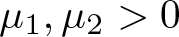
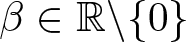
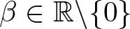
Theorem 1.3 Assume that  $\mu_1,\mu_2 \gt 0$ and
 $\beta\in\mathbb{R}\backslash\{0\}$. If
 $\beta\in (-\infty,-\sqrt{\mu_1\mu_2})\cup(-\sqrt{\mu_1\mu_2},0)\cup(0,\infty)$, then all the curl-free solutions of system (1.10) must be trivial. If
 $\beta=-\sqrt{\mu_1\mu_2}$, then problem (1.10) admits infinitely many fully non-trivial curl-free solutions.
Next, we consider the general case. First, we will try to search for the ground state solutions for (1.10). We mean a solution is ground state if it is non-trivial and has the minimal energy among all the non-trivial solutions. In this paper, we prove that (1.10) does admit a non-trivial ground state solution when the coupling coefficient β is positive and small. More precisely, we have the following theorem.
Theorem 1.4 Assume that  $\mu_1,\mu_2 \gt 0$ and
 $0 \lt \beta \lt 5\sqrt{\mu_1\mu_2}$. Then
 $\inf_{\mathcal{N}} I \gt 0$ is attained and hence the system (1.10) admits a non-trivial ground state solution with positive energy, where
 $\mathcal{N}$ is the corresponding Nehari–Pankov manifold to problem (1.10) and will be defined in §3. Moreover, if
 \begin{equation*}
\beta \gt \max \left\{\frac{\sqrt{2}\left(19 \mu_2-\mu_1\right)}{8}, \frac{\sqrt{2}\left(19 \mu_1-\mu_2\right)}{8}\right\} \gt 0,
\end{equation*}
then the ground state solution obtained above must be fully non-trivial.
For general  $\beta\in\mathbb{R}\backslash\{0\}$, since the term in the energy functional corresponding to the nonlinear term of system (1.10) is no longer convex, it is very difficult to find a ground state solution. So we will try to find cylindrically symmetric solutions.
Theorem 1.5 Assume that  $\mu_1,\mu_2 \gt 0$ and
 $\beta\in\mathbb{R}\backslash\{0\}$. Then the system (1.10) admits a non-trivial cylindrically symmetric solution, and it has positive least energy among all solutions of such form.
Remark 1.6. One can see from the proof of Theorem 1.4 that if
 \begin{equation*}
\beta \gt \max \left\{\frac{\sqrt{2}\left(19 \mu_2-\mu_1\right)}{8}, \frac{\sqrt{2}\left(19 \mu_1-\mu_2\right)}{8}\right\} \gt 0,
\end{equation*}
then the least energy cylindrically symmetric solution obtained in Theorem 1.5 must also be fully non-trivial.
Finally, we give some comments on synchronized solutions of system (1.10), i.e., solutions of the form (su, tu) with  $s,t\in\mathbb{R}$. Let u be the solution of problem (1.7). Since the system (1.10) is
 $(\mathbb{Z}_2\times\mathbb{Z}_2)$-invariant, we will find the synchronized solution
 $(u_1,u_2)$ of the form
 $(\sqrt{k}u,\sqrt{l}u)$ for
 $k,l\in\mathbb{R}_+$. In particular, we have the following result.
Theorem 1.7 Assume that  $\mu_1,\mu_2 \gt 0$ and
 $\beta\in\mathbb{R}\backslash\{0\}$, then (1.10) admits infinitely many synchronized solutions of the form
 $(\sqrt{k}u,\sqrt{l}u)$, where u is a solution of (1.7) and
 $k,l \gt 0$ satisfy
 \begin{equation}
\begin{cases} \mu_1k^2+\beta k^{\frac{1}{2}}l^{\frac{3}{2}}=1, \\ \beta k^{\frac{3}{2}}l^{\frac{1}{2}}+\mu_2l^2=1.\end{cases}
\end{equation}
The organization of this paper is as follows. In §2, we will consider the curl-free solutions and then prove Theorem 1.3. In §3, we will give a detailed concentration-compactness analysis in  $\mathbb{R}^3$ corresponding to system (1.10) and then prove Theorem 1.4. In §4, we will establish Theorem 1.5 with the help of group action. Finally, we will give the proof of Theorem 1.7 in §5.
2. On the existence and non-existence of non-trivial curl-free solutions
In this section, we will give the proof of Theorem 1.3. To begin with, let us state some facts about the solutions of system (1.10).
Assume that  $(u_1,u_2)$ is a solution of (1.10), then the energy of
 $(u_1,u_2)$ is
 \begin{equation}
\begin{aligned}
I(u_1,u_2)&=\frac{1}{2}\int_{\mathbb{R}^3}\left(|\nabla\times u_1|^2+|\nabla\times u_2|^2\right)\,dx \nonumber\\
&\quad -\frac{1}{6}\int_{\mathbb{R}^3}\left(\mu_1|u_1|^6+\mu_2|u_2|^6+2\beta|u_1|^3|u_2|^3\right)\,dx\\
&=\frac{1}{3}\int_{\mathbb{R}^3}\left(|\nabla\times u_1|^2+|\nabla\times u_2|^2\right)\,dx\\
&=\frac{1}{3}\int_{\mathbb{R}^3}\left(\mu_1|u_1|^6+\mu_2|u_2|^6+2\beta|u_1|^3|u_2|^3\right)\,dx.
\end{aligned}
\end{equation}
Now, using (2.1), we can prove Theorem 1.3 by a detailed analysis.
[Proof of Theorem 1.3] Assume that  $(u_1,u_2)$ is a curl-free solution of (1.10), then we know the energy of
 $(u_1,u_2)$ is zero by (2.1), from which we can easily deduce that
 $(u_1,u_2)$ is trivial if β > 0. When β < 0, the situation becomes more delicate, and we need a more detailed analysis. Since the curl part of u 1 and u 2 is vanishing, we know
 \begin{equation}
\begin{cases}\mu_1|u_1|^4u_1+\beta|u_1||u_2|^3u_1=0 & \text {a.e. in } \mathbb{R}^3, \\ \mu_2|u_2|^4u_2+\beta|u_1|^3|u_2|u_2=0 & \text {a.e. in } \mathbb{R}^3.\end{cases}
\end{equation}
One can easily find out that, except for a subset of  $\mathbb{R}^3$ with Lebesgue measure zero, the following linear system with respect to
 $|u_1|^3$ and
 $|u_2|^3$ holds
 \begin{equation*}
\begin{cases}\mu_1|u_1|^3+\beta|u_2|^3=0,& \\ \mu_2|u_2|^3+\beta|u_1|^3=0.&\end{cases}
\end{equation*}
Based on Cramer’s rule, if the determinant  $\mu_1\mu_2-\beta^2$ is not equal to zero, then the only possibility is that
 $u_1\equiv u_2\equiv 0$. Therefore, we only need to deal with the case when
 $\beta=-\sqrt{\mu_1\mu_2}$. For
 $\beta=-\sqrt{\mu_1\mu_2}$, if
 $(u_1,u_2)$ is a curl-free solution of (1.10), then by the fact that the energy of
 $(u_1,u_2)$ is zero, one has
 \begin{equation*}
\int_{\mathbb{R}^3}\left(\mu_1|u_1|^6+\mu_2|u_2|^6\right)\,dx=2\sqrt{\mu_1\mu_2}\int_{\mathbb{R}^3}|u_1|^3|u_2|^3\,dx.
\end{equation*}
By Hölder’s inequality, we know
 \begin{equation*}
2\sqrt{\mu_1\mu_2}\int_{\mathbb{R}^3}|u_1|^3|u_2|^3\,dx\leq2\left(\mu_1\int_{\mathbb{R}^3}|u_1|^6\,dx\right)^{1/2}\left(\mu_2\int_{\mathbb{R}^3}|u_2|^6\,dx\right)^{1/2}.
\end{equation*}
Again, by the Cauchy–Schwarz inequality, we know
 \begin{equation*}
\begin{aligned}
I(u_1,u_2)&=\frac{1}{3}\int_{\mathbb{R}^3}\left(\mu_1|u_1|^6+\mu_2|u_2|^6-2\sqrt{\mu_1\mu_2}|u_1|^3|u_2|^3\right)\,dx\\
&\geq\frac{1}{3}\int_{\mathbb{R}^3}\left(\mu_1|u_1|^6+\mu_2|u_2|^6\right)\,dx \nonumber\\
&\quad -\frac{2}{3}\left(\mu_1\int_{\mathbb{R}^3}|u_1|^6\,dx\right)^{1/2}\left(\mu_2\int_{\mathbb{R}^3}|u_2|^6\,dx\right)^{1/2}\\
&=\frac{1}{3}\left(\left(\mu_1\int_{\mathbb{R}^3}|u_1|^6\,dx\right)^{1/2}-\left(\mu_2\int_{\mathbb{R}^3}|u_2|^6\,dx\right)^{1/2}\right)^2\\
&\geq 0.
\end{aligned}
\end{equation*}
To ensure the validity of  $I(u_1,u_2)=0$, either
 $u_1\equiv u_2\equiv 0$ or
 \begin{equation}
\mu_1\int_{\mathbb{R}^3}|u_1|^6\,dx=\mu_2\int_{\mathbb{R}^3}|u_2|^6\,dx
\end{equation}
and there exists a positive number c > 0 such that
 \begin{equation}
|u_1|^6=c|u_2|^6,\quad\text{a.e. in }\mathbb{R}^3.
\end{equation}
Combining (2.3) and (2.4), we have  $\mu_2=\mu_1 c$ and thus
 \begin{equation*}
|u_1|=\left(\frac{\mu_2}{\mu_1}\right)^{1/6}|u_2|,\quad\text{a.e. in }\mathbb{R}^3.
\end{equation*}
Finally, for  $k\in\mathbb{N}_+$, take
 \begin{equation*}u_{2,k}(x)=
\begin{cases}-\frac{x}{|x|}, & |x|\leq\frac{1}{k}, \\ 0, & |x| \gt \frac{1}{k},\end{cases}
\end{equation*}
and
 \begin{equation*}
u_{1,k}(x)=\left(\frac{\mu_2}{\mu_1}\right)^{1/6}u_{2,k}(x),\quad x\in\mathbb{R}^3,
\end{equation*}
then one may easily verify for any  $k\in\mathbb{N}_+$ that
 $(u_{1,k},u_{2,k})$ is a fully non-trivial curl-free solution of (1.10), and the statement in Theorem 1.3 for the case of
 $\beta=-\sqrt{\mu_1\mu_2}$ is valid since
 $k\in\mathbb{N}_+$ can be freely chosen.
3. On the concentration-compactness analysis in  $\mathbb{R}^3$ and the ground state solutions

Throughout this section, we always assume that  $0 \lt \beta \lt 5\sqrt{\mu_1\mu_2}$. Define
 \begin{equation}
c_\beta:=\inf_{(v_1,v_2)\in H\backslash\{(0,0)\}}\frac{1}{3}\left(\frac{\int_{\mathbb{R}^3}\left(|\nabla v_1|^2+|\nabla v_2|^2\right)\,dx}{\left(\int_{\mathbb{R}^3}\left(\mu_1|v_1|^6+2\beta|v_1|^3|v_2|^3+\mu_2|v_2|^6\right)\,dx\right)^{\frac{1}{3}}}\right)^{\frac{3}{2}},
\end{equation}
where  $H:= D^{1,2}(\mathbb{R}^3,\mathbb{R}^3)\times D^{1,2}(\mathbb{R}^3,\mathbb{R}^3)$. By the classical Sobolev embedding inequality, it is standard to prove that
 $c_\beta \gt 0$. Define
 \begin{equation*}
E(v_1,v_2):= |\nabla v_1|^2+|\nabla v_2|^2
\end{equation*}
and
 \begin{equation*}
N(v_1,v_2):=\mu_1|v_1|^6+2\beta|v_1|^3|v_2|^3+\mu_2|v_2|^6
\end{equation*}
for simplicity, then
 \begin{equation}
\int_{\mathbb{R}^3}E(v_1,v_2)\,dx\geq (3c_\beta)^{\frac{2}{3}}\left(\int_{\mathbb{R}^3}N(v_1,v_2)\,dx\right)^{\frac{1}{3}},\quad\forall\,(v_1,v_2)\in H.
\end{equation}
To proceed, we first derive an important lemma, which is the counterpart of the Brezis–Lieb Lemma [Reference Brézis and Lie10, Reference Willem42] for  $(v_1,v_2)$.
Lemma 3.1. Let  $\Omega\subset\mathbb{R}^3$ be an open subset and
 $\{(v_{1,n},v_{2,n})\}_{n=1}^\infty\subset L^6(\Omega,\mathbb{R}^3)\times L^6(\Omega,\mathbb{R}^3)$ be a bounded sequence. If
 $(v_{1,n},v_{2,n})\to(v_{1,0},v_{2,0})$ almost everywhere in Ω as
 $n\to\infty$, then
 \begin{equation*}
\lim_{n\to\infty}\int_{\Omega}\left(|v_{1,n}|^3|v_{2,n}|^3-|v_{1,n}-v_{1,0}|^3|v_{2,n}-v_{2,0}|^3\right)\,dx=\int_{\Omega}|v_{1,0}|^3|v_{2,0}|^3\,dx.
\end{equation*}
The proof of Lemma 3.1 comes from [Reference Chen and Zou12], and we present it here for the sake of completeness.
Proof. Fatou’s Lemma yields
 \begin{equation}
\int_{\Omega}|v_{1,0}|^{6} \leq \liminf _{n \rightarrow \infty} \int_{\Omega}|v_{1,n}|^6 \lt \infty,\quad \int_{\Omega}|v_{2,0}|^{6} \leq \liminf _{n \rightarrow \infty} \int_{\Omega}|v_{2,n}|^6 \lt \infty.
\end{equation}
For any  $a_1, b_1, a_2, b_2 \in \mathbb{R}$ and ɛ > 0, we deduce from the Mean Value Theorem and Young’s inequality that
 \begin{equation*}
\begin{aligned}
& \Big| | a_1+b_1|^3|a_2+b_2|^3-|a_1|^3|a_2|^3 \Big| \\
\leq & \Big|| a_1+b_1|^3-|a_1|^3\Big|\cdot | a_2+b_2|^3+|a_1|^3\cdot\Big| |a_2+b_2|^3-|a_2|^3 \Big| \\
\leq & C\left[\left(|a_1|+|b_1|\right)^{2}\left(|a_2|+|b_2|\right)^3|b_1|+|a_1|^3\left(|a_2|+|b_2|\right)^{2}|b_2|\right] \\
\leq & C \varepsilon\left[\left(|a_1|+|b_1|\right)^{6}+\left(|a_2|+|b_2|\right)^{6}\right]+ \frac{C}{\varepsilon^{5}}\left(|b_1|^{6}+|b_2|^{6}\right) \\
\leq & C \varepsilon\left(|a_1|^{6}+|b_1|^{6}+|a_2|^6+|b_2|^{6}\right)+ \frac{C}{\varepsilon^{5}}\left(|b_1|^{6}+|b_2|^{6}\right) .
\end{aligned}
\end{equation*}
Here, C > 0 is a positive constant which is independent of  $\varepsilon, a_i$ and bi,
 $i=1,2$. Denote
 $\omega_{1,n}=v_{1,n}-v_{1,0}$ and
 $\omega_{2,n}=v_{2,n}-v_{2,0}$. Then
 \begin{equation*}
\begin{aligned}
f_n^{\varepsilon} &:= \bigg[\Big||v_{1,n}|^3|v_{2,n}|^3-|\omega_{1,n}|^3|\omega_{2,n}|^3-|v_{1,0}|^3|v_{2,0}|^3 \Big| \nonumber\\
&\quad -C \varepsilon\left(|\omega_{1,n}|^6+|v_{1,0}|^6+|\omega_{2,n}|^6+|v_{2,0}|^6\right)\bigg]_{+} \\
&\leq |v_{1,0}|^3|v_{2,0}|^3+\frac{C}{\varepsilon^5}\left(|v_{1,0}|^6+|v_{2,0}|^6\right),
\end{aligned}
\end{equation*}
and so the Dominated Convergence Theorem yields  $\int_{\Omega} f_n^{\varepsilon} d x \rightarrow 0$ as
 $n \rightarrow \infty$. Note that
 \begin{align*}
&\Big|| v_{1,n}|^3|v_{2,n}|^3-|\omega_{1,n}|^3|\omega_{2,n}|^3-|v_{1,0}|^3|v_{2,0}|^3 \Big| \nonumber\\
&\quad \leq f_n^{\varepsilon}+C \varepsilon\left(|\omega_{1,n}|^6+|v_{1,0}|^6+|\omega_{2,n}|^6+|v_{2,0}|^6\right),
\end{align*}
so we obtain
 \begin{equation*}
\limsup _{n \rightarrow \infty} \int_{\Omega}\Big||v_{1,n}|^3|v_{2,n}|^3-|\omega_{1,n}|^3|\omega_{2,n}|^3-|v_{1,0}|^3|v_{2,0}|^3 \Big|\,dx \leq C \varepsilon
\end{equation*}
by (3.3) and the fact that  $\{(\omega_{1,n},\omega_{2,n})\}_{n=1}^\infty$ is bounded in
 $L^6(\Omega,\mathbb{R}^3)\times L^6(\Omega,\mathbb{R}^3)$. Since C > 0 is independent of ɛ > 0, the proof is complete.
To begin with, let us state some facts, which are important and necessary for the proof of Theorem 1.4. Define
 \begin{align}
&F:\mathbb{R}^3\times\mathbb{R}^3\to\mathbb{R},\quad F(u_1,u_2) \nonumber\\
&\quad :=\frac{1}{6}\big(\mu_1|u_1|^6+2\beta|u_1|^3|u_2|^3+\mu_2|u_2|^6\big),\quad\forall\,u_1,u_2\in\mathbb{R}^3.
\end{align}
For  $\varepsilon_0 \gt 0$, we write
 \begin{equation*}
\begin{aligned}
F(u_1,u_2)&=\varepsilon_0\big(|u_1|^6+|u_2|^6\big)\\
&\quad +\frac{1}{6}\big((\mu_1-6\varepsilon_0)|u_1|^6+2\beta|u_1|^3|u_2|^3+(\mu_2-6\varepsilon_0)|u_2|^6\big)\\
&=: \varepsilon_0 G(u_1,u_2)+H_{\varepsilon_0}(u_1,u_2).
\end{aligned}
\end{equation*}
Since  $0 \lt \beta \lt 5\sqrt{\mu_1\mu_2}$, one can easily verify that the hessian
 $\nabla^2 H_{\varepsilon_0}$ of
 $H_{\varepsilon_0}$ is everywhere positive semi-definite, and hence
 $H_{\varepsilon_0}$ is convex in
 $\mathbb{R}^3\times\mathbb{R}^3$, supposed that
 $\varepsilon_0 \gt 0$ is sufficiently small. Then, one can easily know that the function F is strictly convex with respect to
 $(u_1,u_2)\in\mathbb{R}^3\times\mathbb{R}^3$. In view of the above fact, for any
 $(v_1,v_2)\in\mathcal{V}\times\mathcal{V}$, we can find a unique minimizer
 $(w_1(v_1,v_2),w_2(v_1,v_2))\in\mathcal{W}\times\mathcal{W}$ in the sense that
 \begin{align}
&\int_{\mathbb{R}^3}F(v_1+w_1(v_1,v_2),v_2+w_2(v_1,v_2))\,dx \nonumber\\
&\quad \leq\int_{\mathbb{R}^3}F(v_1+w_1,v_2+w_2)\,dx,\quad\text{for all }(w_1,w_2)\in\mathcal{W}\times\mathcal{W},
\end{align}
and the equality in (3.5) holds if and only if  $(w_1,w_2)=(w_1(v_1,v_2),w_2(v_1,v_2))$. Moreover, this implies that
 \begin{align}
&\int_{\mathbb{R}^3}\langle f_1(v_1+w_1,v_2+w_2),\varphi_1\rangle+\langle f_2(v_1+w_1,v_2+w_2),\varphi_2\rangle\,dx=0, \nonumber\\
&\quad \quad\text{for all }(\varphi_1,\varphi_2)\in\mathcal{W}\times\mathcal{W}
\end{align}
if and only if  $(w_1,w_2)=(w_1(v_1,v_2),w_2(v_1,v_2))$, where
 $(f_1,f_2)$ is the gradient of F. More concretely,
 \begin{equation*}
f_1:=\partial_{u_1}F:\mathbb{R}^3\times\mathbb{R}^3\to\mathbb{R}^3,\quad f_2:=\partial_{u_2}F:\mathbb{R}^3\times\mathbb{R}^3\to\mathbb{R}^3.
\end{equation*}
Denote the space of finite measures in  $\mathbb{R}^3$ by
 $\mathcal{M}(\mathbb{R}^3)$. The following lemma is the counterpart of the concentration-compactness analysis for the curl operator, which is established by Mederski and Szulkin [Reference Mederski and Szulkin27], for problem (1.10).
Lemma 3.2. Let  $\{(v_{1,n},v_{2,n})\}_{n=1}^\infty\subset\mathcal{V}\times\mathcal{V}$ be a sequence such that
 \begin{equation}
\begin{cases} (v_{1,n},v_{2,n})\rightharpoonup (v_{1,0},v_{2,0})\text{ weakly in }\mathcal{V}\times\mathcal{V}, \\
(v_{1,n},v_{2,n})\rightarrow (v_{1,0},v_{2,0})\text{ almost everywhere in }\mathbb{R}^3,\\
E(v_{1,n},v_{2,n})\rightharpoonup \mu\text{ weakly in }\mathcal{M}(\mathbb{R}^3),\\
N(v_{1,n},v_{2,n})\rightharpoonup \rho\text{ weakly in }\mathcal{M}(\mathbb{R}^3).
\end{cases}
\end{equation}
Then there exist an at most countable set  $I\subset\mathbb{R}^3$ and non-negative weights
 $\{\mu_x\}_{x\in I}$,
 $\{\rho_x\}_{x\in I}$ such that
 \begin{equation}
\mu\geq E(v_{1,0},v_{2,0})+\sum_{x\in I}\mu_x\delta_x,\quad\rho= N(v_{1,0},v_{2,0})+\sum_{x\in I}\rho_x\delta_x,
\end{equation}
where δx is the usual Dirac measure at x. Moreover, passing to a subsequence if necessary, we have
 \begin{equation}
\begin{cases}
(w_1(v_{1,n},v_{2,n}),w_2(v_{1,n},v_{2,n}))\rightharpoonup (w_1(v_{1,0},v_{2,0}),w_2(v_{1,0},v_{2,0}))\text{ weakly in } \mathcal{W}\times\mathcal{W},\\
(w_1(v_{1,n},v_{2,n}),w_2(v_{1,n},v_{2,n}))\to(w_1(v_{1,0},v_{2,0}),w_2(v_{1,0},v_{2,0})) \\
\qquad \text{almost everywhere in }\mathbb{R}^3,\\
(w_1(v_{1,n},v_{2,n}),w_2(v_{1,n},v_{2,n}))\to(w_1(v_{1,0},v_{2,0}),w_2(v_{1,0},v_{2,0}))\\
\qquad \text{ strongly in } L_{loc}^p(\mathbb{R}^3)\text{for any }1\leq p \lt 6. \end{cases}
\end{equation}
Proof. In this proof, we mainly follow the arguments of [Reference Mederski and Szulkin27, Theorem 3.1]. First, for any  $\varphi\in C_0^\infty(\mathbb{R}^3)$, by (3.2), we know
 \begin{equation}
\begin{aligned}
&\quad\left(\int_{\mathbb{R}^3}N\big(\varphi (v_{1,n}-v_{1,0}),\varphi (v_{2,n}-v_{2,0})\big)\,dx\right)^{\frac{1}{3}}\\
&\leq (3c_\beta)^{-\frac{2}{3}}\int_{\mathbb{R}^3} E\big(\varphi (v_{1,n}-v_{1,0}), \varphi (v_{2,n}-v_{2,0})\big)\,dx \\
&=(3c_\beta)^{-\frac{2}{3}}\int_{\mathbb{R}^3}|\varphi|^2\big(|\nabla(v_{1,n}-v_{1,0})|^2+|\nabla(v_{2,n}-v_{2,0})|^2\big)\,dx+o_n(1).
\end{aligned}
\end{equation}
Using the classic Brezis–Lieb Lemma [Reference Brézis and Lie10, Reference Willem42] and Lemma 3.1, we obtain
 \begin{equation}
\left(\int_{\mathbb{R}^3}|\varphi|^6\,d\bar{\rho}\right)^{\frac{1}{3}}\leq (3c_\beta)^{-\frac{2}{3}}\int_{\mathbb{R}^3}|\varphi|^2\,d\bar{\mu},
\end{equation}
where  $\bar{\mu}:= \mu-E(v_{1,0},v_{2,0})$ and
 $\bar{\rho}:=\rho-N(v_{1,0},v_{2,0})$. Notice that µ is a finite measure, we know the singular set
 $I:=\{x\in\mathbb{R}^3:\mu_x=\mu(\{x\}) \gt 0\}$ is at most countable and the measures µ and
 $\bar{\mu}$ have the same singular set. Following the arguments of [Reference Evans16, Theorem 1.4.2] or [Reference Waliullah39, Proposition 4.2], one can prove that
 \begin{equation}
\bar{\mu}\geq\sum_{x\in I}\mu_x\delta_x\quad\text{and}\quad\bar{\rho}=\sum_{x\in I}\rho_x\delta_x,
\end{equation}
as claimed.
Now, we prove the second conclusion of Lemma 3.2. For simplicity, we denote
 \begin{equation*}
w_{i,n}=w_i(v_{1,n},v_{2,n}),\,\, u_{i,n}=v_{i,n}+w_{i,n},\,\, \,\,\text{for }i=1,2,\,n\in\mathbb{N}_+.
\end{equation*}
Notice that by the definition of  $(u_{1,n},u_{2,n})$, we have
 \begin{equation*}
\begin{aligned}
\frac{\mu_1}{6}\|u_{1,n}\|_6^6+\frac{\mu_2}{6}\|u_{2,n}\|_6^6&\leq\int_{\mathbb{R}^3}F(u_{1,n},u_{2,n})\,dx\\
&\leq\int_{\mathbb{R}^3}F(v_{1,n},v_{2,n})\,dx\\
&\leq C\big(\|v_{1,n}\|_6^6+\|v_{2,n}\|_6^6\big),
\end{aligned}
\end{equation*}
from which we know  $\{(w_{1,n},w_{2,n})\}_{n=1}^\infty$ is bounded in
 $L^6(\mathbb{R}^3,\mathbb{R}^3)\times L^6(\mathbb{R}^3,\mathbb{R}^3)$, also in
 $\mathcal{W}\times\mathcal{W}$. Therefore, we may assume that
 $(w_{1,n},w_{2,n})\rightharpoonup (w_{1,0},w_{2,0})$ weakly in
 $\mathcal{W}\times\mathcal{W}$ for some
 $(w_{1,0},w_{2,0})\in\mathcal{W}\times\mathcal{W}$.
Denote  $u_{i,0}=v_{i,0}+w_{i,0}$ for
 $i=1,2$ and furthermore, let
 $\{B_k\}_{k=1}^\infty$ be a sequence of open balls such that
 $\cup_{k=1}^\infty B_k=\mathbb{R}^3$. For fixed
 $k\in\mathbb{N}_+$, since Bk is simply connected and
 $\nabla\times w_{1,n}=\nabla\times w_{2,n}\equiv 0$, we can find
 $\xi_{1,n},\xi_{2,n}\in W^{1,6}(B_k)$ such that
 $(w_{1,n},w_{2,n})=(\nabla \xi_{1,n},\nabla\xi_{2,n})$ in view of [Reference Leinfelder20, Lemma 1.1]. Besides, we may assume that
 \begin{equation*}
\int_{B_k}\xi_{1,n}\,dx=\int_{B_k}\xi_{2,n}\,dx=0
\end{equation*}
by adding a constant if necessary. Then by Poincaré inequality, we easily know that  $\{(\xi_{1,n},\xi_{2,n})\}_{n=1}^\infty$ is bounded in
 $W^{1,6}(B_k)\times W^{1,6}(B_k)$. Passing to a subsequence, we can assume that
 $(\xi_{1,n},\xi_{2,n})\rightharpoonup(\xi_{1,0},\xi_{2,0})$ weakly in
 $W^{1,6}(B_k)\times W^{1,6}(B_k)$ for some
 $(\xi_{1,0},\xi_{2,0})\in W^{1,6}(B_k)\times W^{1,6}(B_k)$. Moreover, we know
 $(\xi_{1,n},\xi_{2,n})\rightarrow(\xi_{1,0},\xi_{2,0})$ strongly in
 $L^6(B_k)\times L^6(B_k)$ by Morrey’s Embedding Theorem. For
 $\varphi\in C_0^\infty(B_k)$, since
 $\big(\nabla(|\varphi|^6(\xi_{1,n}-\xi_{1,0})),\nabla(|\varphi|^6(\xi_{2,n}-\xi_{2,0}))\big)\in\mathcal{W}\times\mathcal{W}$, we know from (3.6) that
 \begin{equation}
\begin{aligned}
&\int_{\mathbb{R}^3}\big(\langle f_1(u_{1,n},u_{2,n}),\nabla(|\varphi|^6(\xi_{1,n}-\xi_{1,0}))\rangle\\
&\quad +\langle f_2(u_{1,n},u_{2,n}),\nabla(|\varphi|^6(\xi_{2,n}-\xi_{2,0}))\rangle\big)\,dx=0,
\end{aligned}
\end{equation}
that is,
 \begin{equation}
\begin{aligned}
&\int_{\mathbb{R}^3}|\varphi|^6\big(\langle f_1(u_{1,n},u_{2,n}),w_{1,n}-\nabla\xi_{1,0}\rangle+\langle f_2(u_{1,n},u_{2,n}),w_{2,n}-\nabla\xi_{2,0}\rangle\big)\,dx\\
&=\int_{\mathbb{R}^3}\big(\langle f_1(u_{1,n},u_{2,n}),\nabla(|\varphi|^6)(\xi_{1,0}-\xi_{1,n})\rangle\\
&\quad +\langle f_2(u_{1,n},u_{2,n}),\nabla(|\varphi|^6)(\xi_{2,0}-\xi_{2,n})\rangle\big)\,dx,
\end{aligned}
\end{equation}
where the right-hand side of (3.14) tends to 0 as  $n\to\infty$ since
 $(\xi_{1,n},\xi_{2,n})\rightarrow(\xi_{1,0},\xi_{2,0})$ strongly in
 $L^6(B_k)\times L^6(B_k)$. On the other hand, since
 $(w_{1,n},w_{2,n})\rightharpoonup(\nabla\xi_{1,0},\nabla\xi_{2,0})$ weakly in
 $L^6(B_k,\mathbb{R}^3)\times L^6(B_k,\mathbb{R}^3)$, we know
 \begin{equation}
\begin{aligned}
\int_{\mathbb{R}^3}|\varphi|^6\big(\langle f_1(u_{1,0},u_{2,0}),w_{1,n}-\nabla\xi_{1,0}\rangle
+\langle f_2(u_{1,0},u_{2,0}),w_{2,n}-\nabla\xi_{2,0}\rangle\big)\,dx=o_n(1).
\end{aligned}
\end{equation}
Combining (3.14) and (3.15), we know
 \begin{equation}
\begin{aligned}
\int_{\mathbb{R}^3}|\varphi|^6\big(\langle f_1(u_{1,n}&,u_{2,n})-f_1(u_{1,0},u_{2,0}),w_{1,n}-\nabla\xi_{1,0}\rangle\\
&+\langle f_2(u_{1,n},u_{2,n})-f_2(u_{1,0},u_{2,0}),w_{2,n}-\nabla\xi_{2,0}\rangle\big)\,dx=o_n(1).
\end{aligned}
\end{equation}
Since F is convex, we know
 \begin{equation}
F\left(\frac{u_1+v_1}{2},\frac{u_2+v_2}{2}\right)\geq F(u_1,u_2)+\left\langle f_1(u_1,u_2),\frac{v_1-u_1}{2}\right\rangle+\left\langle f_2(u_1,u_2),\frac{v_2-u_2}{2}\right\rangle
\end{equation}
and
 \begin{equation}
F\left(\frac{u_1+v_1}{2},\frac{u_2+v_2}{2}\right)\geq F(v_1,v_2)+\left\langle f_1(v_1,v_2),\frac{u_1-v_1}{2}\right\rangle+\left\langle f_2(v_1,v_2),\frac{u_2-v_2}{2}\right\rangle.
\end{equation}
For any  $l\in\mathbb{N}_+$, define
 \begin{equation}
m_l:= \inf_{\substack{u_1,u_2,v_1,v_2\in\mathbb{R}^3, \\ |u_1-v_1|+|u_2-v_2|\geq \frac{1}{l},\\ |u_1|,|u_2|,|v_1|,|v_2|\leq l}}\frac{1}{2}\left(F(u_1,u_2)+F(v_1,v_2)\right)-F\left(\frac{u_1+v_1}{2},\frac{u_2+v_2}{2}\right).
\end{equation}
By the analysis before Lemma 3.2, we know
 \begin{equation*}
m_l\geq \varepsilon_0\inf_{\substack{u_1,u_2,v_1,v_2\in\mathbb{R}^3, \\ |u_1-v_1|+|u_2-v_2|\geq \frac{1}{l},\\ |u_1|,|u_2|,|v_1|,|v_2|\leq l}}\frac{1}{2}\left(G(u_1,u_2)+G(v_1,v_2)\right)-G\left(\frac{u_1+v_1}{2},\frac{u_2+v_2}{2}\right) \gt 0,
\end{equation*}
where the positivity of ml is from the fact that  $x\mapsto |x|^6$ is uniformly strictly convex, hence has a modulus of convexity of power type 6 (see [Reference Borwein, Guirao, Hájek and Vanderwerff9, Theorem 2.3]). Here, we say that a convex function
 $\theta:\mathbb{R}^3\to\mathbb{R}$ is uniformly strictly convex if
 \begin{equation*}\delta_\theta(t):=\inf \left\{\frac{1}{2} \theta(x)+\frac{1}{2} \theta(y)-\theta\left(\frac{x+y}{2}\right):\,\|x-y\|=t,\, x, y \in \operatorname{dom} \theta\right\} \gt 0\end{equation*}
for all t > 0. Combining (3.17) and (3.18), one obtains for any  $l\in\mathbb{N}_+$,
 $|u_1-v_1|+|u_2-v_2|\geq \frac{1}{l}$ and
 $|u_1|,|u_2|,|v_1|,|v_2|\leq l$ that
 \begin{equation}
\begin{aligned}
m_l&\leq\frac{1}{2}\left(F(u_1,u_2)+F(v_1,v_2)\right)-F\left(\frac{u_1+v_1}{2},\frac{u_2+v_2}{2}\right)\\
&\leq\frac{1}{4}\big(\langle f_1(u_1,u_2)-f_1(v_1,v_2), u_1-v_1\rangle+\langle f_2(u_1,u_2)-f_2(v_1,v_2), u_2-v_2\rangle\big).
\end{aligned}
\end{equation}
Let
 \begin{equation*}
\begin{aligned}
\Omega_{n,l}:=\bigg\{x\in\mathbb{R}^3:\,|u_{1,n}-u_{1,0}|+|u_{2,n}-u_{2,0}|\\
\geq\frac{1}{l}\text{and }|u_{1,n}|,\,|u_{2,n}|,\,|u_{1,0}|,\,|u_{2,0}|\leq l\bigg\}.
\end{aligned}
\end{equation*}
Taking into account (3.16) and (3.20), we obtain, by Hölder’s inequality, for fixed  $l\in\mathbb{N}_+$ that
 \begin{equation*}
\begin{aligned}
4m_l\int_{\Omega_{n,l}}|\varphi|^6\,dx&\leq \int_{\Omega_{n,l}}|\varphi|^6\big(\langle f_1(u_{1,n},u_{2,n})-f_1(u_{1,0},u_{2,0}),u_{1,n}-u_{1,0}\rangle\\
&\quad+\langle f_2(u_{1,n},u_{2,n})-f_2(u_{1,0},u_{2,0}),u_{2,n}-u_{2,0}\rangle\big)\,dx\\
&\leq \int_{\mathbb{R}^3}|\varphi|^6\big(\langle f_1(u_{1,n},u_{2,n})-f_1(u_{1,0},u_{2,0}),u_{1,n}-u_{1,0}\rangle\\
&\quad+\langle f_2(u_{1,n},u_{2,n})-f_2(u_{1,0},u_{2,0}),u_{2,n}-u_{2,0}\rangle\big)\,dx\\
&= \int_{\mathbb{R}^3}|\varphi|^6\big(\langle f_1(u_{1,n},u_{2,n})-f_1(u_{1,0},u_{2,0}),v_{1,n}-v_{1,0}\rangle\\
&\quad+\langle f_2(u_{1,n},u_{2,n})-f_2(u_{1,0},u_{2,0}),v_{2,n}-v_{2,0}\rangle\big)\,dx+o_n(1)\\
&\leq C\left(\int_{\mathbb{R}^3} N(\varphi(v_{1,n}-v_{1,0}),\varphi(v_{2,n}-v_{2,0}))\,dx\right)^{\frac{1}{6}}+o_n(1)\\
&= C\left(\int_{\mathbb{R}^3}|\varphi|^6\,d\bar{\rho}\right)^{\frac{1}{6}}+o_n(1),
\end{aligned}
\end{equation*}
where we have used the fact that β > 0 again to deduce the last inequality. Since the test function  $\varphi\in C_0^\infty(B_k)$ is arbitrarily chosen, we know
 \begin{equation}
4m_l|\Omega_{n,l}\cap E|\leq C\big(\bar{\rho}(E)\big)^{1/6}+o_n(1)
\end{equation}
for any Borel set  $E\subset B_k$, where the notation
 $|\cdot|$ in (3.21) stands for the usual Lebesgue measure. Recall that I is the singular set of the measure µ, and is a subset of
 $\mathbb{R}^3$ with measure 0. Now, find an open set
 $E_l\supset I$ such that
 $|E_l| \lt 1/2^{l+1}$. Then by taking
 $E=B_k\backslash E_l$, we have
 \begin{equation*}
4m_l|\Omega_{n,l}\cap (B_k\backslash E_l)|=o_n(1),
\end{equation*}
where we have used the fact that  $\operatorname{supp}(\bar{\rho})\subset I$. Therefore, for sufficiently large
 $n_l\in\mathbb{N}_+$, there holds
 \begin{equation*}
|\Omega_{n_l,l}\cap B_k| \lt \frac{1}{2^l},
\end{equation*}
and we obtain that
 \begin{equation*}
\left|\bigcap_{i=1}^\infty\bigcup_{l=i}^\infty \Omega_{n_l,l}\cap B_k\right|\leq\lim_{i\to\infty}\sum_{l=i}^\infty |\Omega_{n_l,l}\cap B_k|\leq\lim_{i\to\infty}\frac{1}{2^{i-2}}=0.
\end{equation*}
If  $x\not\in\cap_{i=1}^\infty\cup_{l=i}^\infty \Omega_{n_l,l}$ and
 $x\in B_k$, we know
 \begin{equation*}
|u_{1,n_l}-u_{1,0}|+|u_{2,n_l}-u_{2,0}| \lt \frac{1}{l},\text{or }|u_{1,n_l}| \gt l,\text{or }|u_{2,n_l}| \gt l,\text{or }|u_{1,0}| \gt l,\text{or }|u_{2,0}| \gt l
\end{equation*}
for all sufficiently large  $l\in\mathbb{N}_+$. Since
 $\{u_{i,n}\}_{n=1}^\infty$ is bounded in
 $L^6(\mathbb{R}^3,\mathbb{R}^3)$ for
 $i=1,2$ and
 $u_{1,0},$
 $u_{2,0}\in L^6(\mathbb{R}^3,\mathbb{R}^3)$, we know all the inequalities above can not hold on a set of positive measure for all large l except for the first one inequality. Then we know that
 $u_{1,n_l}\to u_{1,0}$ and
 $u_{2,n_l}\to u_{2,0}$ almost everywhere in Bk, and hence
 $w_{1,n_l}\to w_{1,0}$ and
 $w_{2,n_l}\to w_{2,0}$ almost everywhere in Bk. Since
 $(w_{1,n},w_{2,n})\rightharpoonup(\nabla\xi_{1,0},\nabla\xi_{2,0})$ weakly in
 $L^6(B_k)\times L^6(B_k)$, we know
 $(w_{1,0},w_{2,0})=(\nabla\xi_{1,0},\nabla\xi_{2,0})$ almost everywhere in Bk. Finally, by employing a standard diagonal procedure, we can find a subsequence of
 $(w_{1,n},w_{2,n})$ which converges to
 $(w_{1,0},w_{2,0})$ almost everywhere in
 $\mathbb{R}^3$.
Let  $p\in[1,6)$. For
 $\Omega\subset\mathbb{R}^3$ such that
 $|\Omega| \lt \infty$, we have
 \begin{equation*}
\int_{\Omega}|u_{i,n}-u_{i,0}|^p\,dx\leq|\Omega|^{1-\frac{p}{6}}\left(\int_{\mathbb{R}^3}|u_{i,n}-u_{i,0}|^6\,dx\right)^{\frac{p}{6}}\leq C,\quad i=1,2.
\end{equation*}
Hence by the Vitali Convergence Theorem, we know  $u_{i,n}\to u_{i,0}$ and hence
 $w_{i,n}\to w_{i,0}$ in
 $L^p_{loc}(\mathbb{R}^3,\mathbb{R}^3)$ for
 $i=1,2$ after selecting a subsequence if necessary.
Finally, we need to prove that  $(w_{1,0},w_{2,0})= (w_1(v_{1,0},v_{2,0}),w_2(v_{1,0},v_{2,0}))$. For any
 $(\varphi_1,\varphi_2)\in\mathcal{W}\times\mathcal{W}$, by Remark 1.1 and the Vitali Convergence Theorem again, we have
 \begin{align*}
0&=\int_{\mathbb{R}^3}\langle f_1(u_{1,n},u_{2,n}),\varphi_1\rangle+\langle f_2(u_{1,n},u_{2,n}),\varphi_2\rangle\,dx\\
&\to\int_{\mathbb{R}^3}\langle f_1(u_{1,0},u_{2,0}),\varphi_1\rangle+\langle f_2(u_{1,0},u_{2,0}),\varphi_2\rangle\,dx
\end{align*}
up to a subsequence if necessary. Therefore, (3.6) implies the desired result.
Now we look for the ground states for the system (1.10). First, we give an important lemma, of which we will make repeated use.
Lemma 3.3. For any  $(v_1,v_2)\in\mathcal{V}\times\mathcal{V}$ and λ > 0, there holds
 \begin{equation*}
(w_1(\lambda v_1,\lambda v_2),w_2(\lambda v_1,\lambda v_2))=(\lambda w_1(v_1,v_2),\lambda w_2(v_1,v_2)).
\end{equation*}
Proof. Using the minimizing property of  $(w_1(v_1,v_2),w_2(v_1,v_2))$, we have
 \begin{equation*}
\begin{aligned}
&\lambda^6\int_{\mathbb{R}^3}F(v_1+w_1(v_1,v_2),v_2+w_2(v_1,v_2))\,dx\\
&\quad =\int_{\mathbb{R}^3}F(\lambda v_1+\lambda w_1(v_1,v_2),\lambda v_2+\lambda w_2(v_1,v_2))\,dx\\
&\quad \geq \int_{\mathbb{R}^3}F(\lambda v_1+ w_1(\lambda v_1,\lambda v_2),\lambda v_2+ w_2(\lambda v_1,\lambda v_2))\,dx\\
&\quad =\lambda^6\int_{\mathbb{R}^3}F( v_1+ w_1(\lambda v_1,\lambda v_2)/\lambda, v_2+ w_2(\lambda v_1,\lambda v_2)/\lambda)\,dx\\
&\quad \geq\lambda^6\int_{\mathbb{R}^3}F(v_1+w_1(v_1,v_2),v_2+w_2(v_1,v_2))\,dx.
\end{aligned}
\end{equation*}
Again by the uniqueness property of  $(w_1(v_1,v_2),w_2(v_1,v_2))$, we get the desired result.
Define the Nehari–Pankov type manifold of system (1.10) as follows
 \begin{equation}
\begin{aligned}
\mathcal{N}&:=\bigg\{(u_1,u_2)\in \big(W_0^6(\operatorname{curl} ; \mathbb{R}^3)\times W_0^6(\operatorname{curl} ; \mathbb{R}^3)\big)\backslash(\mathcal{W}\times\mathcal{W}):\\
&I^\prime(u_1,u_2)[u_1,u_2]=0\text \ \text{and } \ I^\prime(u_1,u_2)|_{\mathcal{W}\times\mathcal{W}}=0\bigg\}.
\end{aligned}
\end{equation}
It follows from (3.5) and (3.6) that for any  $(v_1,v_2)\in\mathcal{V}\times\mathcal{V}$, there holds
 \begin{equation*}
I^\prime\big(v_1+w_1(v_1,v_2),v_2+w_2(v_1,v_2)\big)|_{\mathcal{W}\times\mathcal{W}}=0.
\end{equation*}
Notice that
 \begin{equation*}
\begin{aligned}
I&(t(v_1+w_1(v_1,v_2)),t(v_2+w_2(v_1,v_2)))=\frac{t^2}{2}\int_{\mathbb{R}^3}\big(|\nabla\times v_1|^2+|\nabla\times v_2|^2\big)\,dx\\
&-\frac{t^6}{6}\int_{\mathbb{R}^3}\big(\mu_1|v_1+w_1(v_1,v_2)|^6+2\beta|v_1+w_1(v_1,v_2)|^3|v_2+w_2(v_1,v_2)|^3\\
&\quad +\mu_2|v_2+w_2(v_1,v_2)|^6\big)\,dx.
\end{aligned}
\end{equation*}
Then we know for  $(v_1,v_2)\in(\mathcal{V}\times\mathcal{V})\backslash\{(0,0)\}$, there exists a unique constant
 $t=t_m(v_1,v_2) \gt 0$ such that
 \begin{equation}
m(v_1,v_2):=(t_m(v_1,v_2)(v_1+w_1(v_1,v_2)),t_m(v_1,v_2)(v_2+w_2(v_1,v_2)))\in\mathcal{N},
\end{equation}
where we have used Lemma 3.3 to ensure that  $I^\prime(m(v_1,v_2))|_{\mathcal{W}\times\mathcal{W}}=0$. Notice that for any
 $(w_1,w_2)\in\mathcal{W}\times\mathcal{W}$ and any t > 0, there holds
 \begin{equation}
I(m(v_1,v_2))\geq I(t(v_1+w_1),t(v_2+w_2)).
\end{equation}
In particular, there holds  $I(m(v_1,v_2))\geq I(tv_1,tv_2)$ for any t > 0. Notice that by the Sobolev Embedding Theorem, we know there exist positive constants
 $a,r \gt 0$ such that
 $I(v_1,v_2)\geq a$ if
 $\|(v_1,v_2)\|=r$. Then, it is easy to know
 $\inf_{\mathcal{N}}I \gt 0$, from which we know
 $\mathcal{N}$ is bounded away from
 $\mathcal{W}\times\mathcal{W}$ since
 $I\leq 0$ on
 $\mathcal{W}\times\mathcal{W}$. Besides, we know
 $\mathcal{N}$ is closed due to the same reasoning.
From (3.23), we have actually defined a mapping  $m:(\mathcal{V}\times\mathcal{V})\backslash\{(0,0)\}\to\mathcal{N}$. Next, we will show that this mapping is continuous.
Lemma 3.4. The mapping  $m:(\mathcal{V}\times\mathcal{V})\backslash\{(0,0)\}\to\mathcal{N}$ defined by (3.23) is continuous.
Proof. Suppose that  $(v_{1,n},v_{2,n})\to(v_{1,0},v_{2,0})\neq(0,0)$ in
 $\mathcal{V}\times\mathcal{V}$. Furthermore, denote
 \begin{equation*}
(u_{1,n},u_{2,n})=m(v_{1,n},v_{2,n})=t_m(v_{1,n},v_{2,n})(v_{1,n}+w_{1,n},v_{2,n}+w_{2,n}).
\end{equation*}
Since for  $i=1,2$,
 \begin{equation}
\int_{\mathbb{R}^3}|v_{i,n}+w_{i,n}|^6\,dx\leq C\int_{\mathbb{R}^3}F(v_{1,n}+w_{1,n},v_{2,n}+w_{2,n})\,dx\leq C\int_{\mathbb{R}^3}F(v_{1,n},v_{2,n})\,dx,
\end{equation}
we know  $\{(w_{1,n},w_{2,n})\}_{n=1}^\infty$ is bounded, and then it is clear that so is
 $\{t_m(v_{1,n},v_{2,n})\}_{n=1}^\infty$ by the definition and the Helmholtz decomposition (1.11). Without loss of generality, we may assume that
 $t_m(v_{1,n},v_{2,n})\to t_0$ and
 $(w_{1,n},w_{2,n})\rightharpoonup(w_{1,0},w_{2,0})$ weakly in
 $L^6(\mathbb{R}^3,\mathbb{R}^3)\times L^6(\mathbb{R}^3,\mathbb{R}^3)$. By the weak sequential lower semi-continuity property of the convex functional, we know
 \begin{equation*}
\begin{aligned}
I(t_0(v_{1,0}+w_{1,0}),t_0(v_{2,0}+w_{2,0}))&\geq \limsup_{n \rightarrow \infty}I(u_{1,n},u_{2,n})\\
&\geq\limsup_{n \rightarrow \infty}I(t_0(v_{1,n}+w_{1,0}),t_0(v_{2,n}+w_{2,0}))\\
&=I(t_0(v_{1,0}+w_{1,0}),t_0(v_{2,0}+w_{2,0})).
\end{aligned}
\end{equation*}
Therefore, by Radon’s Theorem, we know  $(w_{1,n},w_{2,n})\to(w_{1,0},w_{2,0})$ strongly in
 $L^6(\mathbb{R}^3,\mathbb{R}^3)\times L^6(\mathbb{R}^3,\mathbb{R}^3)$. Besides, since
 $\mathcal{N}$ is closed, we have
 \begin{equation*}
t_0(v_{1,0}+w_{1,0},v_{2,0}+w_{2,0})=m(v_{1,0},v_{2,0})\in\mathcal{N},
\end{equation*}
and hence Lemma 3.4 is valid.
Let  $(u_1,u_2)=(v_1+w_1,v_2+w_2)\in\mathcal{N}$. Define the inverse of the mapping m by
 \begin{equation*}
m^{-1}:\mathcal{N}\to \mathcal{S},\quad m^{-1}(u_1,u_2)=\frac{(v_1,v_2)}{\|(v_1,v_2)\|},
\end{equation*}
where  $\mathcal{S}:=\{(v_1,v_2)\in\mathcal{V}\times\mathcal{V}:\,\|(v_1,v_2)\|=1\}$. Now it is easily seen that
 $m|_{\mathcal{S}}:\mathcal{S} \to\mathcal{N}$ is a homeomorphism with the inverse m −1 defined above. Next, we give some properties of the composite functional
 $I\circ m=:\hat{\mathcal{I}}$.
Proposition 3.5.  $\hat{\mathcal{I}}\in C^1((\mathcal{V}\times\mathcal{V})\backslash\{(0,0)\},\mathbb{R})$, and
 \begin{equation*}
\hat{\mathcal{I}}^\prime(v_1,v_2)[\eta_1,\eta_2]=\frac{\|(\hat{v}_1,\hat{v}_2)\|}{\|(v_1,v_2)\|}I^\prime(m(v_1,v_2))[\eta_1,\eta_2]
\end{equation*}
for  $(v_1,v_2),$
 $(\eta_1,\eta_2)\in\mathcal{V}\times\mathcal{V}$,
 $(v_1,v_2)\neq (0,0)$, where
 \begin{equation*}
(u_1,u_2):= m(v_1,v_2)=(\hat{v}_1,\hat{v}_2)+(w_1,w_2).
\end{equation*}
Proof. Let  $(\eta_1,\eta_2)\in\mathcal{V}\times\mathcal{V}$. Choose δ > 0 such that
 $(v_1^t,v_2^t):=(v_1,v_2)+t(\eta_1,\eta_2)\in(\mathcal{V}\times\mathcal{V})\backslash\{(0,0)\}$ for all
 $|t| \lt \delta$. Moreover, we write
 \begin{equation*}
(u_1^t,u_2^t):= m(v_1^t,v_2^t)=(s^tv_1^t,s^tv_2^t)+(w_1^t,w_2^t)\in\mathcal{N}
\end{equation*}
with  $s^t \gt 0$ positive constants for any
 $|t| \lt \delta$. Then, we know
 $s^0=\frac{\|(\hat{v}_1,\hat{v}_2)\|}{\|(v_1,v_2)\|}$, and the function
 $(-\delta,\delta)\to\mathbb{R}$,
 $t\mapsto s^t$, is continuous by Lemma 3.4. The definition of the mapping m and the Mean Value Theorem now imply that
 \begin{equation*}
\begin{aligned}
\hat{\mathcal{I}}(v_1^t,&v_2^t)-\hat{\mathcal{I}}(v_1,v_2)=I(u_1^t,u_2^t)-I(u_1,u_2)=I((s^tv_1^t,s^tv_2^t)\\
&\quad +(w_1^t,w_2^t))-I((\hat{v}_1,\hat{v}_2)+(w_1,w_2))\\
&=I((s^tv_1^t,s^tv_2^t)+(w_1^t,w_2^t))-I((s^0{v}_1,s^0{v}_2)+(w_1,w_2))\\
&\leq I((s^tv_1^t,s^tv_2^t)+(w_1^t,w_2^t))-I((s^t{v}_1,s^t{v}_2)+(w_1^t,w_2^t))\\
&=I^\prime ((s^t[v_1+\theta^t(v_1^t-v_1)],s^t[v_2+\theta^t(v_2^t-v_2)])\\
&\quad +(w_1^t,w_2^t))[s^t(v_1^t-v_1),s^t(v_2^t-v_2)]\\
&=s^0tI^\prime((s^0v_1,s^0v_2)+(w_1,w_2))[\eta_1,\eta_2]+o(t)\\
&=s^0tI^\prime(u_1,u_2)[\eta_1,\eta_2]+o(t)\quad\text{as }t\to 0,
\end{aligned}
\end{equation*}
with some  $\theta^t\in(0,1)$. By a similar reasoning, we also have that
 \begin{equation*}
\begin{aligned}
\hat{\mathcal{I}}(v_1^t,&v_2^t)-\hat{\mathcal{I}}(v_1,v_2)=I((s^tv_1^t,s^tv_2^t)+(w_1^t,w_2^t))-I((s^0{v}_1,s^0{v}_2)+(w_1,w_2))\\
&\geq I((s^0v_1^t,s^0v_2^t)+(w_1,w_2))-I((s^0{v}_1,s^0{v}_2)+(w_1,w_2))\\
&=I^\prime ((s^0[v_1+\vartheta^t(v_1^t-v_1)],s^0[v_2+\vartheta^t(v_2^t-v_2)])\\
&\quad +(w_1,w_2))[s^0(v_1^t-v_1),s^0(v_2^t-v_2)]\\
&=s^0tI^\prime((s^0v_1,s^0v_2)+(w_1,w_2))[\eta_1,\eta_2]+o(t)\\
&=s^0tI^\prime(u_1,u_2)[\eta_1,\eta_2]+o(t),\quad\text{as }t\to 0,
\end{aligned}
\end{equation*}
with some  $\vartheta^t\in(0,1)$. Combining these inequalities, we conclude that the directional derivative
 $\partial_{(\eta_1,\eta_2)}\hat{\mathcal{I}}(v_1,v_2)$ exists and is given by
 \begin{align*}
\partial_{(\eta_1,\eta_2)}\hat{\mathcal{I}}(v_1,v_2)&=\lim\limits_{t\to 0}\frac{\hat{\mathcal{I}}(v_1^t,v_2^t)-\hat{\mathcal{I}}(v_1,v_2)}{t}=s^0I^\prime(u_1,u_2)[\eta_1,\eta_2]\\
&=\frac{\|(\hat{v}_1,\hat{v}_2)\|}{\|(v_1,v_2)\|}I^\prime(m(v_1,v_2))[\eta_1,\eta_2].
\end{align*}
Hence we know  $\partial_{(\eta_1,\eta_2)}\hat{\mathcal{I}}(v_1,v_2)$ is linear and continuous in
 $(\eta_1,\eta_2)$ and depends continuously on
 $(v_1,v_2)$. So the assertion follows from [Reference Willem42, Proposition 1.3].
Next, we consider the restriction  $\mathcal{I}:\mathcal{S}\to\mathbb{R}$ of
 $\hat{\mathcal{I}}$ to
 $\mathcal{S}$.
(a).
$\mathcal{I}\in C^1(\mathcal{S})$, and for
$(v_1,v_2)\in\mathcal{S}$, denote
$m(v_1,v_2)=(\hat{v}_1,\hat{v}_2)+(w_1,w_2)$, then we have
\begin{equation*}\nonumber
\mathcal{I}^\prime(v_1,v_2)[\eta_1,\eta_2]=\|(\hat{v}_1,\hat{v}_2)\|I^\prime(m(v_1,v_2))[\eta_1,\eta_2]
\end{equation*}for
\begin{align*}
(\eta_1,\eta_2)\in \mathcal{T}_{(v_1,v_2)}\mathcal{S}&:=\left\{(\xi_1,\xi_2)\in\mathcal{V}\times\mathcal{V} \right.\\
&\quad \left.:\int_{\mathbb{R}^3}\big(\langle\nabla\times v_1,\nabla\times \xi_1\rangle+\langle\nabla\times v_2,\nabla\times \xi_2\rangle\big)\,dx=0\right\}.
\end{align*}(b).
$\{(v_{1,n},v_{2,n})\}_{n=1}^\infty\subset\mathcal{S}$ is a Palais–Smale sequence for
$\mathcal{I}$ if and only if
$\{m(v_{1,n},v_{2,n})\}_{n=1}^\infty$ is a Palais–Smale sequence for I.(c). We have
\begin{equation*}
\inf_{\mathcal{S}}\mathcal{I}=\inf_{\mathcal{N}}I=c_0 \gt 0.
\end{equation*}Moreover,
$(v_1,v_2)\in\mathcal{S}$ is a critical point of
$\mathcal{I}$ if and only if
$m(v_1,v_2)$ is a critical point of I, and the corresponding critical values coincide.


Proof. From Proposition 3.5 and the fact that  $m|_{\mathcal{S}}:\mathcal{S}\to\mathcal{N}$ is a homeomorphism, we only need to prove statement (b). Let
 $\{(v_{1,n},v_{2,n})\}_{n=1}^\infty\subset\mathcal{S}$ be a sequence such that
 \begin{equation}
C_0=\sup_{n}\mathcal{I}(v_{1,n},v_{2,n})=\sup_{n}I(m(v_{1,n},v_{2,n})) \lt \infty,
\end{equation}
and let  $(u_{1,n},u_{2,n}):= m(v_{1,n},v_{2,n})=(\hat{v}_{1,n},\hat{v}_{2,n})+(w_{1,n},w_{2,n})\in\mathcal{N}$. Denote
 \begin{align*}
E(u_1,u_2)&:=\mathbb{R}(u_1,u_2)+(\mathcal{W}\times\mathcal{W})\text{for }(u_1,u_2)\in\big(W_0^6(\operatorname{curl} ; \mathbb{R}^3)\\
&\quad \times W_0^6(\operatorname{curl} ; \mathbb{R}^3)\big)\backslash(\mathcal{W}\times\mathcal{W}).
\end{align*}
Then by the Orthogonal Decomposition Theorem, we have for every  $n\in\mathbb{N}_+$ that
 \begin{equation*}
W_0^6(\operatorname{curl} ; \mathbb{R}^3)\times W_0^6(\operatorname{curl} ; \mathbb{R}^3)=E(v_{1,n},v_{2,n})\oplus\mathcal{T}_{(v_{1,n},v_{2,n})}\mathcal{S}=E(u_{1,n},u_{2,n})\oplus\mathcal{T}_{(v_{1,n},v_{2,n})}\mathcal{S}.
\end{equation*}
Besides, since  $I^\prime(u_{1,n},u_{2,n})[\eta_1,\eta_2]=0$ for all
 $(\eta_1,\eta_2)\in E(u_{1,n},u_{2,n})$, we find out that
 \begin{equation*}
\begin{aligned}
\|\mathcal{I}^\prime(v_{1,n},v_{2,n})\|&=\sup_{\substack{(\eta_1,\eta_2)\in\mathcal{T}_{(v_{1,n},v_{2,n})}\mathcal{S}\\ \|(\eta_1,\eta_2)\|=1}}\mathcal{I}^\prime(v_{1,n},v_{2,n})[\eta_1,\eta_2]\\
&=\sup_{\substack{(\eta_1,\eta_2)\in\mathcal{T}_{(v_{1,n},v_{2,n})}\mathcal{S}\\ \|(\eta_1,\eta_2)\|=1}}\|(\hat{v}_{1,n},\hat{v}_{2,n})\|I^\prime(u_{1,n},u_{2,n})[\eta_1,\eta_2]\\
&=\|(\hat{v}_{1,n},\hat{v}_{2,n})\|\cdot\|I^\prime(u_{1,n},u_{2,n})\|.
\end{aligned}
\end{equation*}
Since  $(u_{1,n},u_{2,n})\in\mathcal{N}$, we have
 \begin{equation*}
\begin{aligned}
I(u_{1,n},u_{2,n})&=\frac{1}{3}\int_{\mathbb{R}^3}\big(|\nabla\times u_{1,n}|^2+|\nabla\times u_{2,n}|^2\big)\,dx\\
&=\frac{1}{3}\int_{\mathbb{R}^3}\big(|\nabla\times \hat{v}_{1,n}|^2+|\nabla\times \hat{v}_{2,n}|^2\big)\,dx\geq \inf_{\mathcal{N}}I \gt 0,
\end{aligned}
\end{equation*}
and
 \begin{equation*}
\begin{aligned}
I(u_{1,n},u_{2,n})=\frac{1}{3}\int_{\mathbb{R}^3}\big(|\nabla\times \hat{v}_{1,n}|^2+|\nabla\times \hat{v}_{2,n}|^2\big)\,dx\leq C_0,
\end{aligned}
\end{equation*}
where C 0 is defined in (3.26). Combining the above two inequalities, we know
 \begin{equation*}
0 \lt \sqrt{3\inf_{\mathcal{N}}I}\leq\|(\hat{v}_{1,n},\hat{v}_{2,n})\|\leq\sqrt{3C_0} \lt \infty,
\end{equation*}
and hence  $\{(v_{1,n},v_{2,n})\}_{n=1}^\infty\subset\mathcal{S}$ is a Palais–Smale sequence for
 $\mathcal{I}$ if and only if
 $\{m(v_{1,n},v_{2,n})\}_{n=1}^\infty$ is a Palais–Smale sequence for I.
For s > 0,  $y\in\mathbb{R}^3$, and
 $u_1,u_2:\mathbb{R}^3\to\mathbb{R}^3$, we denote
 $T_{s,y}(u_1,u_2):= s^{1/2}(u_1(s\cdot+y),u_2(s\cdot+y))$. We have the next two lemmas, as a counterpart of [Reference Mederski and Szulkin27, Lemma 4.5] and [Reference Mederski and Szulkin27, Lemma 4.6].
Lemma 3.7. Suppose that  $\{(v_{1,n},v_{2,n})\}_{n=1}^\infty\subset H$ is bounded, where H is defined in the beginning of § 3. Then
 $(v_{1,n},v_{2,n})\to 0$ strongly in
 $L^6(\mathbb{R}^3,\mathbb{R}^3)\times L^6(\mathbb{R}^3,\mathbb{R}^3)$ if and only if
 $T_{s_n,y_n}(v_{1,n},v_{2,n})\rightharpoonup 0$ weakly in H for all
 $\{s_n\}_{n=1}^\infty\subset\mathbb{R}_+$ and
 $\{y_n\}_{n=1}^\infty\subset\mathbb{R}^3$.
Proof. This lemma is a direct generalization of [Reference Mederski and Szulkin27, Lemma 4.5], so we omit the proof here.
Lemma 3.8.  $T_{s,y}$ is an isometric isomorphism of
 $W_0^6(\operatorname{curl} ; \mathbb{R}^3)\times W_0^6(\operatorname{curl} ; \mathbb{R}^3)$ which leaves the functional I and the subspaces
 $\mathcal{V}\times\mathcal{V}$ and
 $\mathcal{W}\times\mathcal{W}$ invariant. In particular, we have
 \begin{equation*}
(w_1(T_{s,y}(u_1,u_2)),w_2(T_{s,y}(u_1,u_2)))=T_{s,y}(w_1(u_1,u_2),w_2(u_1,u_2)).
\end{equation*}
Proof. The proof of this lemma is by an explicit and simple calculation, so we again leave the details to the readers.
Now, we are ready to prove Theorem 1.4.
Proof of Theorem 1.4
By the classic Ekeland Variational Principle [Reference Willem42], there exists a Palais–Smale sequence  $\{(v_{1,n},v_{2,n})\}_{n=1}^\infty\subset\mathcal{S}$ for
 $\mathcal{I}$ such that
 \begin{equation*}
\mathcal{I}(v_{1,n},v_{2,n})\to\inf_{\mathcal{S}}\mathcal{I}=\inf_{\mathcal{N}}I=c_0 \gt 0\quad\text{as }n\to \infty.
\end{equation*}
Besides, it follows from Corollary 3.6 that  $\{(u_{1,n},u_{2,n})\}_{n=1}^\infty\subset\mathcal{N}$ is a Palais–Smale sequence for I on
 $\mathcal{N}$ with
 $I^\prime(u_{1,n},u_{2,n})\to 0$ and
 $I(u_{1,n},u_{2,n})\to c_0$ as
 $n\to\infty$ where for every
 $n\in\mathbb{N}_+$
 \begin{equation*}
(u_{1,n},u_{2,n}):= m(v_{1,n},v_{2,n})=(\hat{v}_{1,n},\hat{v}_{2,n})+(w_{1,n},w_{2,n}).
\end{equation*}
As
 \begin{equation}
\begin{aligned}
I(u_{1,n},u_{2,n})&=I(u_{1,n},u_{2,n})-\frac{1}{6}I^\prime(u_{1,n},u_{2,n})[u_{1,n},u_{2,n}]\\
&=\frac{1}{3}\int_{\mathbb{R}^3}\big(|\nabla\times \hat{v}_{1,n}|^2+|\nabla\times \hat{v}_{2,n}|^2\big)\,dx,
\end{aligned}
\end{equation}
we know  $\{(\hat{v}_{1,n},\hat{v}_{2,n})\}_{n=1}^\infty\subset\mathcal{V}\times\mathcal{V}$ is bounded. On the other hand, we also have
 \begin{equation}
\begin{aligned}
I(u_{1,n},u_{2,n})&=I(u_{1,n},u_{2,n})-\frac{1}{2}I^\prime(u_{1,n},u_{2,n})[u_{1,n},u_{2,n}]\\
&=\frac{1}{3}\int_{\mathbb{R}^3}\big(\mu_1|u_{1,n}|^6+2\beta|u_{1,n}|^3|u_{2,n}|^3+\mu_2|u_{2,n}|^6\big)\,dx.
\end{aligned}
\end{equation}
Since  $I(u_{1,n},u_{2,n})$ is bounded away from 0 by the fact that
 $I(u_{1,n},u_{2,n})\to c_0 \gt 0$, we know by (3.25) and the definition of the mapping m that there exists a constant c > 0, which is independent of n, such that
 \begin{equation*}
\int_{\mathbb{R}^3}\big(|\hat{v}_{1,n}|^6+|\hat{v}_{2,n}|^6\big)\,dx\geq c.
\end{equation*}
Therefore, passing to a subsequence if necessary and using Lemma 3.7, we can assume that
 \begin{equation*}
(\tilde{v}_{1,n},\tilde{v}_{2,n}):= T_{s_n,y_n}(\hat{v}_{1,n},\hat{v}_{2,n})\rightharpoonup(v_{1,0},v_{2,0})\text{weakly in }D^{1,2}(\mathbb{R}^3,\mathbb{R}^3)\times D^{1,2}(\mathbb{R}^3,\mathbb{R}^3)
\end{equation*}
for some  $(v_{1,0},v_{2,0})\neq (0,0)$,
 $\{s_n\}_{n=1}^\infty\subset\mathbb{R}_+$ and
 $\{y_n\}_{n=1}^\infty\subset\mathbb{R}^3$. Suppose that
 $(\tilde{v}_{1,n},\tilde{v}_{2,n})\to(v_{1,0},v_{2,0})$ almost everywhere in
 $\mathbb{R}^3$ after choosing a subsequence if necessary. In view of Lemma 3.2, we have
 \begin{equation*}
\begin{aligned}
(w_1(\tilde{v}_{1,n},\tilde{v}_{2,n}),w_2(\tilde{v}_{1,n},\tilde{v}_{2,n}))&\rightharpoonup (w_1(v_{1,0},v_{2,0}),w_2(v_{1,0},v_{2,0}))\text{weakly in }\mathcal{W}\times\mathcal{W},\\
(w_1(\tilde{v}_{1,n},\tilde{v}_{2,n}),w_2(\tilde{v}_{1,n},\tilde{v}_{2,n}))&\to (w_1(v_{1,0},v_{2,0}),w_2(v_{1,0},v_{2,0}))\\
\quad \text{almost everywhere in }\mathbb{R}^3.
\end{aligned}
\end{equation*}
Set  $(w_{1,0},w_{2,0})=(w_1(v_{1,0},v_{2,0}),w_2(v_{1,0},v_{2,0}))$ and
 $(u_{1,0},u_{2,0})=(v_{1,0},v_{2,0})+(w_{1,0},w_{2,0})$. In view of Lemma 3.8, we may assume without loss of generality that
 $s_n=1$ and
 $y_n=0$ for
 $n\in\mathbb{N}_+$. Now, for
 $(\varphi_1,\varphi_2)\in W_0^6(\operatorname{curl} ; \mathbb{R}^3)\times W_0^6(\operatorname{curl} ; \mathbb{R}^3)$, we know
 \begin{equation*}
\begin{aligned}
I^\prime(u_{1,n},u_{2,n})[\varphi_1,\varphi_2]&=\int_{\mathbb{R}^3}\langle\nabla\times u_{1,n},\nabla\times \varphi_1\rangle\,dx+\int_{\mathbb{R}^3}\langle\nabla\times u_{2,n},\nabla\times \varphi_2\rangle\,dx\\
&\quad-\mu_1\int_{\mathbb{R}^3}|u_{1,n}|^4\langle u_{1,n},\varphi_1\rangle\,dx-\mu_2\int_{\mathbb{R}^3}|u_{2,n}|^4\langle u_{2,n},\varphi_2\rangle\,dx\\
&\quad-\beta\int_{\mathbb{R}^3}|u_{1,n}||u_{2,n}|^3\langle u_{1,n},\varphi_1\rangle\,dx\\
&\quad -\beta\int_{\mathbb{R}^3}|u_{1,n}|^3|u_{2,n}|\langle u_{2,n},\varphi_2\rangle\,dx\\
&\to I^\prime(u_{1,0},u_{2,0})[\varphi_1,\varphi_2]\text{as }n\to\infty.
\end{aligned}
\end{equation*}
Here we have used the fact that  $|u_{i,n}|^4u_{i,n}\rightharpoonup\zeta_i$ in
 $L^{6/5}(\mathbb{R}^3,\mathbb{R}^3)$ for some ζi but since
 $|u_{i,n}|^4u_{i,n}\to|u_{i,0}|^4u_{i,0}$ almost everywhere in
 $\mathbb{R}^3$, we have
 $\zeta_i=|u_{i,0}|^4u_{i,0}$,
 $i=1,2$. For the same reasoning, one can deal with the remaining two terms
 $|u_{1,n}||u_{2,n}|^3u_{1,n}$ and
 $|u_{1,n}|^3|u_{2,n}|u_{2,n}$ since these two terms are also
 $L^{6/5}$-integrable. Therefore, we know
 $(u_{1,0},u_{2,0})$ is actually a non-trivial solution of problem (1.10).
To prove it is a ground state, one notices that by Fatou’s Lemma,
 \begin{equation*}
\begin{aligned}
\inf_{\mathcal{N}}I&=I(u_{1,n},u_{2,n})+o_n(1)\\
&=\frac{1}{3}\int_{\mathbb{R}^3}\big(\mu_1|u_{1,n}|^6+2\beta|u_{1,n}|^3|u_{2,n}|^3+\mu_2|u_{2,n}|^6\big)\,dx+o_n(1)\\
&\geq\frac{1}{3}\int_{\mathbb{R}^3}\big(\mu_1|u_{1,0}|^6+2\beta|u_{1,0}|^3|u_{2,0}|^3+\mu_2|u_{2,0}|^6\big)\,dx+o_n(1)\\
&=I(u_{1,0},u_{2,0})-\frac{1}{2} I^\prime(u_{1,0},u_{2,0})[u_{1,0},u_{2,0}]+o_n(1)=I(u_{1,0},u_{2,0})+o_n(1).
\end{aligned}
\end{equation*}
Therefore, we know  $I(u_{1,0},u_{2,0})\leq\inf_{\mathcal{N}} I$ and since
 $(u_{1,0},u_{2,0})\in\mathcal{N}$, we know
 $(u_{1,0},u_{2,0})$ is a non-trivial ground state solution of (1.10) with positive energy.
Now we prove that the ground state solution obtained above must be fully non-trivial provided
 \begin{equation*}
\beta \gt \max \left\{\frac{\sqrt{2}\left(19 \mu_2-\mu_1\right)}{8}, \frac{\sqrt{2}\left(19 \mu_1-\mu_2\right)}{8}\right\} \gt 0.
\end{equation*}
In fact, we only need to prove that
 \begin{equation}
\inf_{\mathcal{N}}I \lt \min\left\{{\mu_1^{-1/2}},{\mu_2^{-1/2}}\right\}S_{\rm scalar},
\end{equation}
where S scalar is the ground state energy of the scalar problem (1.7). Suppose that  $0 \lt \mu_1\leq \mu_2$. Define
 $\zeta:\mathbb{R}_+\to\mathbb{R}$ as follows
 \begin{equation}
\zeta(t):=\frac{1+t^2}{(\mu_2+2\beta t^3+\mu_1t^6)^{1/3}},\quad t\geq0.
\end{equation}
From a basic calculation, we know
 \begin{equation*}
\lim_{t\to 0_+}\zeta(t)=\zeta(0)=\frac{1}{\mu_2^{1/3}}\leq\frac{1}{\mu_1^{1/3}}=\lim_{t\to\infty}\zeta(t),
\end{equation*}
and there exists  $t_{\rm min}\in[0,\infty)$ such that
 \begin{equation*}
0 \lt \zeta(t_{\rm min})=\min_{t\geq0}\zeta(t)\leq\frac{1}{\mu_2^{1/3}}.
\end{equation*}
Notice that Ye and Peng [Reference Ye and Peng43, Lemma 2.2 and Page 317] proved that
 \begin{equation*}
t_{\rm min} \gt 0\quad\text{and}\quad\zeta(t_{\rm min}) \lt \zeta(0)=\frac{1}{\mu_2^{1/3}}\quad\text{if}\quad \beta \gt \frac{\sqrt{2}\left(19 \mu_2-\mu_1\right)}{8}.
\end{equation*}
Now let u 0 be a non-trivial ground state solution of (1.7). By noticing the identity  $\mu_2+\beta t_{\min }^{3}-\beta t_{\min }-\mu_1 t_{\min }^4=0$, which is a by-product of the definition of t min, we know
 \begin{equation*}
(u_1,u_2):=\left(t_{\rm min}(\mu_2+\beta t_{\rm min}^3)^{-1/4}u_0,(\mu_2+\beta t_{\rm min}^3)^{-1/4}u_0\right)
\end{equation*}
is a solution of (1.10). Moreover, again by this identity, we have
 \begin{equation*}
\begin{aligned}
\inf_{\mathcal{N}}I&\leq I(u_1,u_2)\\
&=\frac{1}{3}\int_{\mathbb{R}^3}\left(|\nabla\times u_1|^2+|\nabla\times u_2|^2\right)\,dx\\
&=(1+t_{\rm min}^2)\cdot(\mu_2+\beta t_{\rm min}^3)^{-1/2}\cdot\frac{1}{3}\int_{\mathbb{R}^3}\left(|\nabla\times u_0|^2\right)\,dx\\
&=(1+t_{\rm min}^2)\cdot\left[\frac{\mu_2+2\beta t_{\rm min}^3+\mu_1 t_{\rm min}^6}{1+t_{\rm min}^2}\right]^{-1/2}\cdot S_{\rm scalar}\\
&=\frac{(1+t_{\rm min}^2)^{3/2}}{(\mu_2+2\beta t_{\rm min}^3+\mu_1 t_{\rm min}^6)^{1/2}}\cdot S_{\rm scalar}\\
&=[\zeta(t_{\min})]^{3/2}\cdot S_{\rm scalar}\\
& \lt \mu_2^{-1/2}S_{\rm scalar}.
\end{aligned}
\end{equation*}
Finally, by the symmetry of the parameters µ 1 and µ 2, we know Theorem 1.4 is valid.
4. On the cylindrically symmetric solutions
In this section, we will establish Theorem 1.5. The symmetry argument used in this section is due to [Reference Clapp and Pistoia14, Reference Ding15, Reference Gaczkowski, Mederski and Schino17, Reference Wen and Zhao40]. Besides, to find a solution with the property of cylindrical symmetry, we will slightly change the definition of the solution. By a solution to (1.10), we mean a critical point  $(u_1,u_2)\in H={D}^{1,2}(\mathbb{R}^3, \mathbb{R}^3)\times D^{1,2}(\mathbb{R}^3,\mathbb{R}^3)$ of I on H.
For convenience, we first provide some notations and definitions. Let  $\pi:\mathbb{S}^3\backslash\{N\}\to\mathbb{R}^3$ be the stereographic projection, where
 $N=(0,0,0,1)\in\mathbb{R}^4$ is the north pole. Define
 \begin{equation*}
\varphi:\mathbb{R}^3\to\mathbb{R},\quad\varphi(x):=\sqrt{\frac{2}{1+|x|^2}},\text{for }x\in\mathbb{R}^3,
\end{equation*}
then explicitly,
 \begin{equation*}
\pi(\xi)=\frac{1}{1-\xi_4}(\xi_1,\xi_2,\xi_3),\text{for }\xi=(\xi_1,\xi_2,\xi_3,\xi_4)\in\mathbb{S}^3\backslash\{N\},
\end{equation*}
and
 \begin{equation*}
\pi^{-1}(x)=\frac{1}{1+|x|^2}(2x_1,2x_2,2x_3,|x|^2-1),\text{for }x=(x_1,x_2,x_3)\in\mathbb{R}^3.
\end{equation*}
Let  $\mathcal{SO}(2)$ be the usual special orthogonal group in dimension 2, and for
 $g\in\mathcal{SO}(2)$, we denote
 \begin{equation*}
\tilde{g}=\left(\begin{array}{ll}g & 0 \\ 0 & 1\end{array}\right) \in \mathcal{S O}:=\mathcal{S O}(2) \times\{1\}.
\end{equation*}
First, we define the group action
 \begin{equation*}
\mathcal{SO}\times H\to H:\quad(u_1,u_2)\mapsto (g^{-1}u_1(g\cdot),g^{-1}u_2(g\cdot))\quad\text{for }g\in\mathcal{SO}\text{and }(u_1,u_2)\in H.
\end{equation*}
Now we define the subspace of invariant points under the above  $\mathcal{SO}$ group action as follows:
 \begin{equation*}
H_{\mathcal{SO}}:=\{(u_1,u_2)\in H:\,(u_1,u_2)=(g^{-1}u_1(g\cdot),g^{-1}u_2(g\cdot))\text{for every }g\in\mathcal{SO}\}.
\end{equation*}
It is immediate that the action of  $\mathcal{SO}$ on H is isometric. Furthermore, for
 $g\in\mathcal{SO}$ and
 $u\in D^{1,2}(\mathbb{R}^3,\mathbb{R}^3)$, we have
 $\nabla\times g^{-1}u(gx)=g^{-1}(\nabla\times u)(gx)$ and
 $|g^{-1}u(gx)|=|u(gx)|$ (see [Reference Azzollini, Benci, D’Aprile and Fortunato2]), then it is easily deduced that the functional I is invariant under the above
 $\mathcal{SO}$ group action. Therefore, by Palais’ principle of symmetric criticality [Reference Palais29, Reference Willem42], every critical point of
 $I|_{H_\mathcal{SO}}$ is also a critical point of I on H. Next, we will introduce a new group G acting on
 $H_\mathcal{SO}$, and we will apply Palais’ principle of symmetric criticality again to the functional
 $I|_{H_\mathcal{SO}}$ to find the critical point of I on H. As in [Reference Azzollini, Benci, D’Aprile and Fortunato2, Lemma 1] and [Reference Bartsch, Dohnal, Plum and Reichel4, Lemma 2.2], we have the following decomposition lemma:
Lemma 4.1. Let  $(u_1,u_2)\in H_\mathcal{SO}$. Then there are unique measurable functions
 $u_{1,\rho},u_{1,\tau},u_{1,\zeta}:(0,\infty)\times\mathbb{R}\to\mathbb{R}$ and
 $u_{2,\rho},u_{2,\tau},u_{2,\zeta}:(0,\infty)\times\mathbb{R}\to\mathbb{R}$ such that
 \begin{align*}
u_1(x)&=\frac{u_{1,\rho}(r,x_3)}{r}\left(\begin{array}{c}x_1 \\ x_2 \\ 0\end{array}\right)+\frac{u_{1,\tau}(r,x_3)}{r}\left(\begin{array}{c}-x_2 \\ x_1 \\ 0\end{array}\right)+\left(\begin{array}{c}0 \\ 0 \\ u_{1,\zeta}(r,x_3)\end{array}\right)\\
&=: U_{1,\rho}+U_{1,\tau}+U_{1,\zeta}
\end{align*}
and
 \begin{align*}
u_2(x)&=\frac{u_{2,\rho}(r,x_3)}{r}\left(\begin{array}{c}x_1 \\ x_2 \\ 0\end{array}\right)+\frac{u_{2,\tau}(r,x_3)}{r}\left(\begin{array}{c}-x_2 \\ x_1 \\ 0\end{array}\right)+\left(\begin{array}{c}0 \\ 0 \\ u_{2,\zeta}(r,x_3)\end{array}\right)\\
&=: U_{2,\rho}+U_{2,\tau}+U_{2,\zeta},
\end{align*}
where  $r:=\sqrt{x_1^2+x_2^2}$.
Now we are ready to define the new group action G on  $H_\mathcal{SO}$.
Lemma 4.2. Define the mapping
 \begin{equation*}
g_1:\left\{\begin{array}{c}
H_\mathcal{SO} \rightarrow H_\mathcal{SO} \\
(u_1,u_2)=(U_{1,\rho}+U_{1,\tau}+U_{1,\zeta},U_{2,\rho}+U_{2,\tau}+U_{2,\zeta})\\
\mapsto (-U_{1,\rho}+U_{1,\tau}-U_{1,\zeta},-U_{2,\rho}+U_{2,\tau}-U_{2,\zeta}).
\end{array}\right.
\end{equation*}
The mapping g 1 is a linear isometry and satisfies  $g_1 \circ g_1=I d$. Hence the generated group
 $G=\left\{I d, g_1\right\}\approx\mathbb{Z}_2$ is of order 2. Moreover, the functional
 $I|_{H_{\mathcal{SO}}}$ is invariant under the action of G.
We omit the proof of this lemma because it is contained in [Reference Azzollini, Benci, D’Aprile and Fortunato2, Proposition 1]. Now, define the space
 \begin{equation*}
H_\mathcal{SO}^G:=\{(u_1,u_2)\in H_{\mathcal{SO}}:g_1(u_1,u_2)=(u_1,u_2)\}=\operatorname{Fix}(G).
\end{equation*}
It results
 \begin{equation*}
H_\mathcal{SO}^G=\{(u_1,u_2)\in H_\mathcal{SO}:(u_1,u_2)=(U_{1,\tau},U_{2,\tau})\},
\end{equation*}
so the elements of  $H_\mathcal{SO}^G$ have the favorable property of being divergence free. Specifically, for
 $(u_1,u_2)\in H_\mathcal{SO}^G$, we have
 $\operatorname{div}(u_1)=\operatorname{div}(u_2)=0$ and thus
 \begin{equation*}
\nabla\times(\nabla \times u_1)=-\Delta u_1,\quad \nabla\times(\nabla \times u_2)=-\Delta u_2.
\end{equation*}
Moreover, for  $(u_1,u_2)\in H_{\mathcal{SO}}^G$, there holds
 \begin{equation*}
\begin{aligned}
I(u_1,u_2)&=\frac{1}{2}\int_{\mathbb{R}^3}|\nabla\times u_1|^2\,dx+\frac{1}{2}\int_{\mathbb{R}^3}|\nabla\times u_2|^2\,dx\\
&\quad-\frac{\mu_1}{6}\int_{\mathbb{R}^3}|u_1|^6\,dx-\frac{\mu_2}{6}\int_{\mathbb{R}^3}|u_2|^6\,dx-\frac{\beta}{3}\int_{\mathbb{R}^3}|u_1|^3|u_2|^3\,dx\\
&=\frac{1}{2}\int_{\mathbb{R}^3}|\nabla u_1|^2\,dx+\frac{1}{2}\int_{\mathbb{R}^3}|\nabla u_2|^2\,dx\\
&\quad-\frac{\mu_1}{6}\int_{\mathbb{R}^3}|u_1|^6\,dx-\frac{\mu_2}{6}\int_{\mathbb{R}^3}|u_2|^6\,dx-\frac{\beta}{3}\int_{\mathbb{R}^3}|u_1|^3|u_2|^3\,dx.
\end{aligned}
\end{equation*}
By Lemma 4.2 and Palais’ principle of symmetric criticality again, we know every critical point of  $I|_{H_\mathcal{SO}^G}$ is also a critical point of
 $I|_{H_\mathcal{SO}}$, hence a critical point of I on H. For a sub-critical problem, the symmetric property of the elements in
 ${H_\mathcal{SO}^G}$ is good enough for us. However, in order to deal with the critical nonlinearity, we need to introduce a new function space with preferred symmetry. For simplicity, denote
 $\mathcal{H}=H_\mathcal{SO}^G$. We introduce the following
 $\mathcal{SO}(2)\times\mathcal{SO}(2)$-group action on
 $\mathcal{H}$.
Definition 4.3. For  $g_1, g_2 \in \mathcal{S O}(2)$ we denote
 $g=\left(\begin{array}{cc}g_1 & 0 \\ 0 & g_2\end{array}\right) \equiv\left(g_1, g_2\right) \in \mathcal{S O}(2) \times$
 $\mathcal{S O}(2)$. We say that the vector field
 $(u_1,u_2) \in \mathcal{H}$ is
 $\mathcal{S O}(2) \times \mathcal{S O}(2)$-symmetric if and only if
 \begin{equation*}
\frac{u_1\big(\pi(g^{-1} \pi^{-1}(x))\big)}{\varphi\big(\pi(g^{-1} \pi^{-1}(x))\big)}=\frac{\widetilde{g_1}^{-1} u_1(x)}{\varphi(x)}\quad\text{and}\quad \frac{u_2\big(\pi(g^{-1} \pi^{-1}(x))\big)}{\varphi\big(\pi(g^{-1} \pi^{-1}(x))\big)}=\frac{\widetilde{g_1}^{-1} u_2(x)}{\varphi(x)}
\end{equation*}
for every  $g_1, g_2 \in \mathcal{S O}(2)$ and for a.e.
 $x \in \mathbb{R}^3$.
The subspace of  $\mathcal{S O}(2) \times \mathcal{S O}(2)$-symmetric vector fields is denoted by
 $\mathcal{H}_{\mathcal{S O}(2) \times \mathcal{S O}(2)}$, and the next lemma reveals that this type of symmetric property can restore the compactness of the classic Sobolev embedding.
Lemma 4.4. The embedding  $\mathcal{H}_{\mathcal{S O}(2) \times \mathcal{S O}(2)}\hookrightarrow L^6(\mathbb{R}^3,\mathbb{R}^3)\times L^6(\mathbb{R}^3,\mathbb{R}^3)$ is compact.
Proof. Notice that in this paper, the notation  $\mathcal{H}_{\mathcal{S O}(2) \times \mathcal{S O}(2)}$ is just a closed subspace of vector space represented by the notation
 $\mathcal{D}_{\mathcal{S O}(2) \times \mathcal{S O}(2)}\times\mathcal{D}_{\mathcal{S O}(2) \times \mathcal{S O}(2)}$ used in [Reference Gaczkowski, Mederski and Schino17]. Therefore, this lemma follows directly from [Reference Gaczkowski, Mederski and Schino17, Lemma 3.2].
Let  $(\mathbb{S}^3,h)$ be the standard sphere and take
 \begin{equation*}
\left(\int_{\mathbb{S}^3}\left(|\nabla_h \mathtt{u}|_h^2+\frac{3}{4}|\mathtt{u}|^2\right)\,d\operatorname{vol}_h\right)^{1/2}
\end{equation*}
as the norm in  $H^1(\mathbb{S}^3,\mathbb{R}^3)$. Notice that the standard metric is given by
 $h_{ij}=\varphi^4\delta_{ij}$. For
 $(u_1,u_2)\in H$, define a mapping
 $\iota:H\to H^1(\mathbb{S}^3,\mathbb{R}^3)\times H^1(\mathbb{S}^3,\mathbb{R}^3)$ by
 \begin{equation*}
(\mathtt{u}_1(\xi),\mathtt{u}_2(\xi))=\iota(u_1,u_2)(\xi):=\left( \frac{u_1(\pi(\xi))}{\varphi(\pi(\xi))},\frac{u_2(\pi(\xi))}{\varphi(\pi(\xi))} \right)\quad\text{for }\xi\in\mathbb{S}^3\backslash\{N\}.
\end{equation*}
One can easily verify that the mapping ι is a linear isometry between H and  $H^1(\mathbb{S}^3,\mathbb{R}^3)\times H^1(\mathbb{S}^3,\mathbb{R}^3)$ and between
 $L^6(\mathbb{R}^3,\mathbb{R}^3)\times L^6(\mathbb{R}^3,\mathbb{R}^3)$ and
 $L^6(\mathbb{S}^3,\mathbb{R}^3)\times L^6(\mathbb{S}^3,\mathbb{R}^3)$, see [Reference Clapp and Pistoia14] for instance. Besides, it is straightforward to verify that
 \begin{equation*}
\int_{\mathbb{S}^3}|\mathtt{u}_1|^3|\mathtt{u}_2|^3\,d\operatorname{vol}_h=\int_{\mathbb{R}^3}|u_1|^3|u_2|^3\,dx.
\end{equation*}
Moreover, since  $\mathbb{S}^3$ is invariant under the action of the group O(4) of linear isometries of
 $\mathbb{R}^4$ (see [Reference Clapp and Pistoia14]), each
 $g=(g_1,g_2)\in \mathcal{SO}(2)\times \mathcal{SO}(2)$ induces a linear isometry
 $g_{iso}:H^1(\mathbb{S}^3,\mathbb{R}^3)\times H^1(\mathbb{S}^3,\mathbb{R}^3)\to H^1(\mathbb{S}^3,\mathbb{R}^3)\times H^1(\mathbb{S}^3,\mathbb{R}^3)$ given by
 \begin{equation*}
g_{iso}(\mathtt{u}_1,\mathtt{u}_2)(\xi):= (\widetilde{g_1}\mathtt{u}_1(g^{-1}\xi),\widetilde{g_1}\mathtt{u}_2(g^{-1}\xi)).
\end{equation*}
Therefore, the composition  $\iota^{-1}\circ g_{iso}\circ\iota: H\to H$ given by
 \begin{equation*}
(u_1(x),u_2(x))\mapsto \left(\frac{\varphi(x)\cdot\widetilde{g_1} u_1\big(\pi(g^{-1} \pi^{-1}(x))\big)}{\varphi\big(\pi(g^{-1} \pi^{-1}(x))\big)},\frac{\varphi(x)\cdot\widetilde{g_1} u_2\big(\pi(g^{-1} \pi^{-1}(x))\big)}{\varphi\big(\pi(g^{-1} \pi^{-1}(x))\big)}\right)
\end{equation*}
is a linear isometry, from which one knows that the  $\mathcal{SO}(2)\times\mathcal{SO}(2)$-group action is an isometry on
 $\mathcal{H}$. Besides, by using the property of the mappings ι and giso, similar as [Reference Gaczkowski, Mederski and Schino17] and [Reference Clapp and Pistoia14], one can easily verify that
 $I|_{\mathcal{H}}$ is invariant under the
 $\mathcal{SO}(2)\times\mathcal{SO}(2)$-group action. Therefore, by Palais’ principle of symmetric criticality, one finally knows that every critical point of
 $I|_{\mathcal{H}_{\mathcal{SO}(2)\times\mathcal{SO}(2)}}$ is also a critical point of I on H, hence a solution of (1.10). Now, we will apply the classic critical point theory to find the solution of (1.10).
Proof of Theorem 1.5
Define the cylindrically symmetric solution manifold as follows
 \begin{equation}
\mathcal{P}:=\{(u_1,u_2)\in\mathcal{H}_{\mathcal{SO}(2)\times\mathcal{SO}(2)}\backslash\{(0,0)\}:I^\prime (u_1,u_2)=0\}.
\end{equation}
It is easy to know that  $\mathcal{P}$ is not empty by the existence of a semi-trivial cylindrically symmetric solution [Reference Gaczkowski, Mederski and Schino17, Theorem 1.2], or by the classic Mountain Pass Theorem [Reference Struwe33, Reference Willem42] with a standard variational procedure. Let
 \begin{equation*}
c_\mathcal{P}:=\inf_{(u_1,u_2)\in\mathcal{P}}I(u_1,u_2).
\end{equation*}
We will prove that  $c_{\mathcal{P}}$ can be attained by some element in
 $\mathcal{P}$. First, we prove that
 $c_{\mathcal{P}} \gt 0$. For any
 $(u_1,u_2)\in\mathcal{P}$ and any
 $t\in(0,\infty)$, by a direct derivative calculation, there holds
 \begin{equation*}
\begin{aligned}
I(u_1,u_2)\geq I(tu_1,tu_2).
\end{aligned}
\end{equation*}
By Lemma 4.4, we know there exist positive constants  $a,r \gt 0$ such that
 $I(u_1,u_2)\geq a$ for any
 $\|(u_1,u_2)\|=r$,
 $(u_1,u_2)\in\mathcal{P}$. Then, it is easy to know
 $c_{\mathcal{P}} \gt 0$. Now, let
 $\{(u_{1,n},u_{2,n})\}_{n=1}^\infty\subset \mathcal{P}$ be a minimizing sequence for
 $c_{\mathcal{P}} \gt 0$, we know
 \begin{equation*}
\begin{aligned}
c_{\mathcal{P}}+o_n(1)&=I(u_{1,n},u_{2,n})\\
&=I(u_{1,n},u_{2,n})-\frac{1}{6}I^\prime(u_{1,n},u_{2,n})[u_{1,n},u_{2,n}]\\
&=\frac{1}{3}\int_{\mathbb{R}^3}|\nabla u_{1,n}|^2\,dx+\frac{1}{3}\int_{\mathbb{R}^3}|\nabla u_{2,n}|^2\,dx.
\end{aligned}
\end{equation*}
Hence, we know  $\{(u_{1,n},u_{2,n})\}_{n=1}^\infty$ is bounded and we can assume that
 $(u_{1,n},u_{2,n})\rightharpoonup (u_{1,0},u_{2,0})$ weakly in
 $\mathcal{H}_{\mathcal{SO}(2)\times\mathcal{SO}(2)}$. From Lemma 4.4, we know that
 $(u_{1,n},u_{2,n})\to (u_{1,0},u_{2,0})$ strongly in
 $L^6(\mathbb{R}^3,\mathbb{R}^3)\times L^6(\mathbb{R}^3,\mathbb{R}^3)$ up to a subsequence. Therefore, it is easy to verify that
 $(u_{1,0},u_{2,0})$ belongs to
 $\mathcal{P}$ and
 $I(u_{1,0},u_{2,0})=c_\mathcal{P}$, i.e.,
 $(u_{1,0},u_{2,0})$ is the desired cylindrically symmetric solution who has positive least energy among all the cylindrically symmetric solutions.
5. On the synchronized solutions
In [Reference Chen and Zou13], Chen and Zou proved that
 \begin{equation*}\nonumber
\begin{cases} \mu_1k^{p-1}+\beta k^{\frac{p}{2}-1}l^{\frac{p}{2}}=1, \\ \beta k^{\frac{p}{2}}l^{\frac{p}{2}-1}+\mu_2l^{p-1}=1,\\ k \gt 0,\,\, l \gt 0\end{cases}
\end{equation*}
has a positive solution (k, l) under the condition p < 2. Their results did not cover the existence result of solution for (1.15). Therefore, we need to first prove that system (1.15) does admit a solution.
Lemma 5.1. Suppose that  $\mu_1,\mu_2 \gt 0$ and
 $\beta\in\mathbb{R}\backslash\{0\}$, then the algebraic system (1.15) has at least one positive solution
 $(k_0,l_0)$.
Proof. From the first equation in (1.15), we know
 \begin{equation*}
l=\left(\frac{1-\mu_1k^2}{\beta k^{\frac{1}{2}}}\right)^{\frac{2}{3}}.
\end{equation*}
By the second equation in (1.15) and to make sure l > 0, we only need to prove that the function
 \begin{equation*}
h(k):=\beta k^{\frac{3}{2}}\left(\frac{1-\mu_1k^2}{\beta k^{\frac{1}{2}}}\right)^{\frac{1}{3}}+\mu_2\left(\frac{1-\mu_1k^2}{\beta k^{\frac{1}{2}}}\right)^{\frac{4}{3}}-1
\end{equation*}
has a zero point  $k\in(0,\mu_1^{-\frac{1}{2}})$. Notice that
 \begin{equation*}
\lim_{k\to 0_+}h(k)=\infty\quad\text{and}\quad\lim_{k\to \mu_1^{-1/2}}h(k)=-1 \lt 0,
\end{equation*}
we immediately get that h(k) must have at least one zero point  $k_0\in(0,\mu_1^{-\frac{1}{2}})$. Besides, it is straightforward to verify that
 \begin{equation*}
l_0=\left(\frac{1-\mu_1k_0^2}{\beta k_0^{\frac{1}{2}}}\right)^{\frac{2}{3}} \gt 0
\end{equation*}
and  $(k_0,l_0)$ is a positive solution of (1.15).
Now, we are ready to prove Theorem 1.7.
Proof of Theorem 1.7
Let u be a solution of (1.7). Suppose that (1.10) admits a solution  $(u_1,u_2)$ of the form
 $(\sqrt{k}u,\sqrt{l}u)$ with
 $k,l \gt 0$, then there holds
 \begin{equation*}
\begin{cases} \nabla \times(\nabla \times u)=(\mu_1k^2+\beta k^{\frac{1}{2}}l^{\frac{3}{2}})|u|^4u & \text {in } \mathbb{R}^3, \\ \nabla \times(\nabla \times u)=(\mu_2l^2+\beta k^{\frac{3}{2}}l^{\frac{1}{2}})|u|^4u & \text {in } \mathbb{R}^3.\end{cases}
\end{equation*}
Therefore, we know  $(\sqrt{k}u,\sqrt{l}u)$ is a solution of (1.10) if and only if (k, l) is a positive solution of the algebraic system (1.15). Finally, Theorem 1.7 follows from Lemma 5.1 and the fact that (1.7) admits infinitely many non-trivial solutions, which is due to [Reference Gaczkowski, Mederski and Schino17, Theorem 1.2].
Acknowledgements
The author would like to thank the referee for valuable comments.
Data availability
No data was used for the research described in the article.



