1. Introduction
The addition of polymer chains to a fluid flow can change the flow properties significantly. A well-known effect is the reduction of drag by polymers in turbulent wall-bounded flows, which was discovered by Toms (Reference Toms1948). The effect of polymers on heat transport is much less studied. In Benzi, Ching & De Angelis (Reference Benzi, Ching and De Angelis2010), using both direct numerical simulations (DNS) and shell model calculations, it was shown that polymer additives can significantly enhance heat transport in homogeneous turbulent thermal convection with no boundaries. At variance with such theoretical results, experiments on turbulent Rayleigh–Bénard (RB) convection of water at moderate Rayleigh numbers (
 $Ra$
),
 $5\times 10^{9}\leqslant Ra\leqslant 7\times 10^{10}$
(Ahlers & Nikolaenko Reference Ahlers and Nikolaenko2010), show that the addition of polymers reduces heat transport, and the amount of reduction increases with polymer concentration. To account for these experimental findings, in a previous paper (Benzi, Ching & Chu Reference Benzi, Ching and Chu2012) some of the authors have generalized the Prandtl–Blasius–Pohlhausen theory to study heat transport by boundary layer flow with polymers using the Oldroyd-B model (Bird et al.
Reference Bird, Hassager, Armstrong and Curtis1987), in which polymer chains can be stretched indefinitely without a limit. We recall that the classical Prandtl–Blasius–Pohlhausen boundary layer theory (Landau & Liftshitz Reference Landau and Lifshitz1987; Schlichting & Gersten Reference Schlichting and Gersten2004) was developed for steady-state forced convection above a semi-infinite weakly heated plate, and has been shown (Grossmann & Lohse Reference Grossmann and Lohse2000; Ahlers, Grossmann & Lohse Reference Ahlers, Grossmann and Lohse2009) to provide a basic understanding of the physics of heat transport in fluctuating boundary layers in turbulent RB convection at moderate
 $Ra$
.
Our previous work demonstrated that polymers give rise to a space-dependent effective viscosity in boundary layer flow. A variable or space-dependent viscosity caused by the temperature dependence of viscosity has been discussed (Cebeci Reference Cebeci2002; Ahlers et al. Reference Ahlers, Brown, Fontenele, Funfschilling, Grossmann and Lohse2006) in strongly turbulent RB convection of Newtonian fluid when non-Boussinesq effects are important. In our previous work, the zero-shear viscosity of the polymer solution is independent of temperature and the space dependence of the effective viscosity arises because of the stretching of the polymers. For Oldroyd-B polymers, the effective viscosity vanishes rather quickly as one moves away from the plate, and is non-zero only within a region very close to the plate. In this case, a reduction in heat transport is found, and the amount of heat reduction increases with the polymer concentration, in agreement with the experimental observations by Ahlers & Nikolaenko (Reference Ahlers and Nikolaenko2010).
More recently, using a convection cell with rough top and bottom plates, Wei, Ni & Xia (Reference Wei, Ni and Xia2012) showed that when polymers are added to water at
 $10^{8}<Ra\leqslant 10^{10}$
, heat transport is first reduced and then enhanced when the polymer concentration is increased. An enhancement in heat transport has also been observed numerically (Dubief Reference Dubief2010) in DNS of turbulent RB convection by polymers described by the finitely extensible nonlinear elastic-Peterlin (FENE-P) model (Bird et al.
Reference Bird, Hassager, Armstrong and Curtis1987) with suitable parameters.
The above numerical and experimental findings motivate our present work. In particular, we extend our generalized Prandtl–Blasius–Pohlhausen boundary layer theory to study how heat transport is affected by finitely extensible polymers described by the FENE-P model. Both the Oldroyd-B and FENE-P models are feasible macroscopic models for numerical studies of polymer drag reduction in turbulent wall-bounded flows (Sureshkumar et al.
Reference Sureshkumar, Beris and Handler1997; Min et al.
Reference Min, Yoo, Choi and Joseph2003). In the FENE-P model, there is an additional parameter
 $b^{2}$
, which is the ratio of the maximum to the equilibrium value of the trace of the polymer conformation tensor and measures the finite extensibility of the polymers. In the limit of
 $b\rightarrow \infty$
, the FENE-P model reduces to the Oldroyd-B model. In Dubief (Reference Dubief2010), a transition from heat reduction to heat enhancement has been observed numerically when
 $b^{2}$
becomes small. We speculate that such a transition is similar in nature to the one observed experimentally by Wei, Ni & Xia (Reference Wei, Ni and Xia2012), and that it can be explained by our generalized Prandtl–Blasius–Pohlhausen boundary layer theory for the FENE-P polymers presented in this paper.
The remainder of this paper is organized as follows. In § 2, we first review our previous work (Benzi et al.
Reference Benzi, Ching and Chu2012) explaining our approach of solving the problem with the Oldroyd-B model. Then we discuss how to extend our approach to study polymers described by the FENE-P model. Using our approach, we calculate the effective viscosity profile and study how the modification in heat transport depends on the three parameters of the problem, namely the finite extensibility parameter
 $b^{2}$
, the Weissenberg number
 $Wi$
, which is the ratio of the polymer relaxation time to the typical time scale of the flow, and
 ${\it\gamma}$
, which is the fraction of the polymer contribution to the zero-shear viscosity of the solution which increases with polymer concentration (see below for the precise definitions of
 $Wi$
and
 ${\it\gamma}$
). In § 3, we present and discuss our results. We show that heat transport is reduced for very large
 $b^{2}$
, as found in our previous study (Benzi et al.
Reference Benzi, Ching and Chu2012) using Oldroyd-B polymers, and the new result that heat transport is enhanced when
 $b^{2}$
is small. By modelling the effective viscosity profile using an analytical mathematical form, we show that the transition from heat reduction to heat enhancement can be explained in terms of the functional shape of the space-dependent effective viscosity. Finally, we summarize and conclude our paper in § 4.
2. Formulation of the problem
For Oldroyd-B polymers, which can be stretched indefinitely without a limit, the problem has been set up in Benzi et al. (Reference Benzi, Ching and Chu2012). In the present paper, we discuss how to extend the formulation to FENE-P polymers.
2.1. Without polymers
For completeness and to define notations, we first summarize the classic Prandtl–Blasius–Pohlhausen theory for steady-state boundary layer flow without polymers above a semi-infinite weakly heated plate. The equations of motion for the steady-state velocity and temperature fields are given by (Landau & Liftshitz Reference Landau and Lifshitz1987; Schlichting & Gersten Reference Schlichting and Gersten2004)
 $$\begin{eqnarray}\displaystyle & \displaystyle \partial _{x}v_{x}+\partial _{y}v_{y}=0, & \displaystyle\end{eqnarray}$$
 $$\begin{eqnarray}\displaystyle & \displaystyle v_{x}\partial _{x}v_{x}+v_{y}\partial _{y}v_{x}={\it\nu}\partial _{yy}^{2}v_{x}, & \displaystyle\end{eqnarray}$$
 $$\begin{eqnarray}\displaystyle & \displaystyle v_{x}\partial _{x}T+v_{y}\partial _{y}T={\it\kappa}\partial _{yy}^{2}T. & \displaystyle\end{eqnarray}$$
Here,
 $x$
denotes the direction along the plate,
 $y$
denotes the direction away from the plate,
 $\partial _{x}$
denotes a partial derivative with respect to
 $x$
,
 $v_{x}(x,y)$
and
 $v_{y}(x,y)$
are the components of the velocity field,
 $T(x,y)$
is the temperature field, and
 ${\it\nu}$
and
 ${\it\kappa}$
are respectively the kinematic viscosity and the thermal diffusivity of the Newtonian fluid. The crucial point about boundary layer flow is that the flow changes more rapidly away from the plate than along the plate, such that
 $\partial _{y}\gg \partial _{x}$
. This condition is satisfied in flows with large Reynolds numbers. Both
 $v_{x}$
and
 $v_{y}$
vanish at the plate, and
 $v_{x}$
merges with the uniform mainstream velocity
 $U$
far away from the plate. The plate is kept at a temperature
 $T_{1}$
above the ambient temperature
 $T_{0}$
far away from the plate. The continuity equation (2.1) is automatically satisfied by introducing the streamfunction
 ${\it\Psi}(x,y)$
, such that
 $v_{x}=\partial _{y}{\it\Psi}$
and
 $v_{y}=-\partial _{x}{\it\Psi}$
. By defining the dimensionless variable
 $$\begin{eqnarray}{\it\xi}\equiv \sqrt{\frac{U}{{\it\nu}_{r}x}}y\end{eqnarray}$$
for some reference kinematic viscosity
 ${\it\nu}_{r}$
and writing
 ${\it\Psi}(x,y)$
and
 $T(x,y)$
in terms of two to-be-determined functions
 ${\it\phi}({\it\xi})$
and
 ${\it\theta}({\it\xi})$
,
 $$\begin{eqnarray}\displaystyle & \displaystyle {\it\Psi}(x,y)=\sqrt{{\it\nu}_{r}xU}{\it\phi}({\it\xi}), & \displaystyle\end{eqnarray}$$
 $$\begin{eqnarray}\displaystyle & \displaystyle T(x,y)=T_{0}+(T_{1}-T_{0}){\it\theta}({\it\xi}), & \displaystyle\end{eqnarray}$$
(2.2) and (2.3) can be reduced to two ordinary differential equations,
 $$\begin{eqnarray}\displaystyle & \displaystyle \frac{1}{2}{\it\phi}{\it\phi}^{\prime \prime }+\left(\frac{{\it\nu}}{{\it\nu}_{r}}\right){\it\phi}^{\prime \prime \prime }=0, & \displaystyle\end{eqnarray}$$
 $$\begin{eqnarray}\displaystyle & \displaystyle 2{\it\theta}^{\prime \prime }+\left(\frac{{\it\nu}_{r}}{{\it\kappa}}\right){\it\phi}{\it\theta}^{\prime }=0. & \displaystyle\end{eqnarray}$$
We use the superscript
 $^{\prime }$
to denote a derivative with respect to
 ${\it\xi}$
. Taking
 ${\it\nu}_{r}={\it\nu}$
, (2.7) gives the famous Blasius equation for velocity,
 $$\begin{eqnarray}{\textstyle \frac{1}{2}}{\it\phi}{\it\phi}^{\prime \prime }+{\it\phi}^{\prime \prime \prime }=0.\end{eqnarray}$$
Solving (2.7) and (2.8) together with the boundary conditions
 $$\begin{eqnarray}{\it\phi}(0)={\it\phi}^{\prime }(0)=0,\quad {\it\phi}^{\prime }(\infty )=1,\end{eqnarray}$$
 $$\begin{eqnarray}{\it\theta}(0)=1,\quad {\it\theta}(\infty )=0\end{eqnarray}$$
we obtain the velocity and temperature profiles,
 ${\it\phi}({\it\xi})$
and
 ${\it\theta}({\it\xi})$
. It is common to measure the heat flux transported from the plate, denoted by
 $Q$
, using the dimensionless Nusselt number (
 $Nu$
) (Landau & Liftshitz Reference Landau and Lifshitz1987), defined by
 $$\begin{eqnarray}Nu\equiv \displaystyle \frac{Q}{2k(T_{1}-T_{0})/L}=\frac{\displaystyle -\!\int _{0}^{L}\left.\frac{\partial T}{\partial y}\right|_{y=0}\,\text{d}x}{2(T_{1}-T_{0})}=\sqrt{\frac{UL}{{\it\nu}_{r}}}~[-{\it\theta}^{\prime }(0)],\end{eqnarray}$$
where
 $k$
is the thermal conductivity of the fluid and
 $L$
is the length of the large plate in the
 $x$
direction.
2.2. The space-dependent effective viscosity produced by Oldroyd-B polymers and its calculation
When polymers are added, they produce an additional stress tensor
 $\unicode[STIX]{x1D61B}_{ij}$
, whose divergence appears as an additional term in the momentum equation (2.2). This polymeric stress depends on how much the polymer chains are stretched and is thus a function of the polymer conformation tensor. Let
 $\boldsymbol{d}$
be the end-to-end vector of a polymer chain. The dimensionless polymer conformation tensor
 $\unicode[STIX]{x1D619}_{ij}(x,y)$
is the average of
 $d_{i}d_{j}/d_{0}^{2}$
over an ensemble of polymer chains in a small region centred at the point
 $(x,y)$
, where
 $d_{0}^{2}$
is the equilibrium value of the ensemble average of
 $d_{x}^{2}$
as well as the ensemble average of
 $d_{y}^{2}$
in the unstretched regime. For the FENE-P model (Bird et al.
Reference Bird, Hassager, Armstrong and Curtis1987), which is based on a dumbbell description of a polymer chain of two equal masses connected by a finitely extensible and nonlinear entropic spring, the functional dependence of
 $\unicode[STIX]{x1D61B}_{ij}$
on
 $\unicode[STIX]{x1D619}_{ij}$
is given by
 $$\begin{eqnarray}\unicode[STIX]{x1D61B}_{ij}=\frac{{\it\nu}_{p}}{{\it\tau}}[P(R)\unicode[STIX]{x1D619}_{ij}-{\it\delta}_{ij}].\end{eqnarray}$$
Here,
 ${\it\tau}$
is the relaxation time of the polymers,
 ${\it\nu}_{p}$
is the polymer contribution to the viscosity of the solution at zero shear, and increases with the concentration of the polymers, and
 $P(R)$
is the Peterlin function
 $$\begin{eqnarray}P(R)=\frac{b^{2}-1}{b^{2}-R/R_{0}},\end{eqnarray}$$
where
 $R=\unicode[STIX]{x1D619}_{xx}+\unicode[STIX]{x1D619}_{yy}$
is the trace of the polymer conformation tensor and the equilibrium value of the trace is
 $R_{0}=2$
. We neglect the extension of the polymer chain in the
 $z$
direction, as it is negligible in two-dimensional boundary layer flow. When
 $R/R_{0}\rightarrow b^{2}$
,
 $P(R)\rightarrow \infty$
and the force required for further extension of the polymer chain becomes infinite. The Peterlin function therefore restricts the maximum value of
 $R$
to be
 $b^{2}R_{0}$
. Thus,
 $b^{2}$
is the ratio of the maximum to the equilibrium value of the trace of the polymer conformation tensor, and measures the finite extensibility of the polymer chains. In the limit
 $b\rightarrow \infty$
,
 $P(R)\rightarrow 1$
, and the FENE-P model reduces to the Oldroyd-B model.
In the presence of FENE-P polymers, (2.2) is modified to
 $$\begin{eqnarray}v_{x}\partial _{x}v_{x}+v_{y}\partial _{y}v_{x}={\it\nu}_{s}\partial _{yy}^{2}v_{x}+\frac{{\it\nu}_{p}}{{\it\tau}}(\partial _{x}\unicode[STIX]{x1D619}_{xx}+\partial _{y}\unicode[STIX]{x1D619}_{xy}),\end{eqnarray}$$
where
 ${\it\nu}_{s}$
denotes the kinematic viscosity of the Newtonian fluid, usually water, before polymers are added. The evolution equations for
 $\unicode[STIX]{x1D619}_{ij}$
,
 $i,j=x$
and
 $y$
, are given by
 $$\begin{eqnarray}v_{x}\partial _{x}\unicode[STIX]{x1D619}_{ij}+v_{y}\partial _{y}\unicode[STIX]{x1D619}_{ij}=\mathop{\sum }_{k=x,y}(\unicode[STIX]{x1D619}_{ik}\partial _{k}v_{j}+\partial _{k}v_{i}\unicode[STIX]{x1D619}_{kj})-\frac{1}{{\it\tau}}(\unicode[STIX]{x1D619}_{ij}-{\it\delta}_{ij}).\end{eqnarray}$$
It is known from the literature (Olagunju Reference Olagunju2006; Bataller Reference Bataller2008) that applying the transformation (2.4) and (2.5)–(2.15) no longer leads to a similarity solution for velocity, as explicit
 $x$
dependence remains in the equation of
 ${\it\phi}$
. In Benzi et al. (Reference Benzi, Ching and Chu2012), we show that a similarity solution can be obtained when we apply the following approximations:
 $$\begin{eqnarray}\displaystyle v_{y}\approx \frac{1}{2}\sqrt{\frac{{\it\nu}_{r}U}{L}}({\it\xi}{\it\phi}^{\prime }-{\it\phi}), & & \displaystyle\end{eqnarray}$$
 $$\begin{eqnarray}\displaystyle \partial _{x}\approx -\frac{{\it\xi}}{2L}\partial _{{\it\xi}},\quad \partial _{y}\approx \sqrt{\frac{U}{{\it\nu}_{r}L}}\partial _{{\it\xi}}. & & \displaystyle\end{eqnarray}$$
These approximations amount to replacing
 $x$
by
 $L$
in the final equation, and introduce an explicit dependence on
 $L$
or the Reynolds number in the equation. We justify the approximations (2.17) and (2.18a,b
) by noting that they are consistent with the boundary layer description, which is meant to be applicable for
 $x$
being large (such that
 $\partial _{y}\gg \partial _{x}$
). We keep the same mainstream velocity
 $U$
in the presence of polymers, as the possible variation in
 $U$
due to the polymers causes only a minor change in the results (Benzi et al.
Reference Benzi, Ching and Chu2012). The modified Blasius equation is then given by
 $$\begin{eqnarray}-\frac{1}{2}{\it\phi}{\it\phi}^{\prime \prime }=\left(\frac{{\it\nu}_{s}}{{\it\nu}_{r}}\right){\it\phi}^{\prime \prime \prime }+\left(\frac{{\it\nu}_{p}}{{\it\nu}_{r}}\right)\frac{1}{Wi\sqrt{Re}}\left[-\frac{{\it\xi}}{2}(P\unicode[STIX]{x1D619}_{xx})^{\prime }+(P\unicode[STIX]{x1D619}_{xy})^{\prime }\right].\end{eqnarray}$$
Here,
 $Wi$
and
 $Re$
denote respectively the Weissenberg number and the Reynolds number, which are defined by
 $$\begin{eqnarray}Wi\equiv \frac{{\it\tau}U}{L},\quad Re\equiv \frac{UL}{{\it\nu}_{r}}.\end{eqnarray}$$
The form of the temperature equation (2.8) remains unchanged in the presence of polymers, but the velocity
 ${\it\phi}$
is now governed by (2.19) instead of (2.7).
Next, we show that keeping
 $\unicode[STIX]{x1D619}_{xx}$
would lead to an unphysical result. We define
 $$\begin{eqnarray}f_{xx}=\int _{0}^{{\it\xi}}-\frac{s}{2}\partial _{s}(P\unicode[STIX]{x1D619}_{xx})\,\text{d}s=-\frac{{\it\xi}}{2}P\unicode[STIX]{x1D619}_{xx}+\frac{1}{2}\int _{0}^{{\it\xi}}P\unicode[STIX]{x1D619}_{xx}\,\text{d}s,\end{eqnarray}$$
then (2.19) can be rewritten as
 $$\begin{eqnarray}-\frac{1}{2}{\it\phi}{\it\phi}^{\prime \prime }=\left(\frac{{\it\nu}_{s}}{{\it\nu}_{r}}\right){\it\phi}^{\prime \prime \prime }+\left(\frac{{\it\nu}_{p}}{{\it\nu}_{r}}\right)\frac{1}{Wi\sqrt{Re}}(f_{xx}+P\unicode[STIX]{x1D619}_{xy})^{\prime }.\end{eqnarray}$$
The quantity
 $f_{xx}+P\unicode[STIX]{x1D619}_{xy}$
represents the polymeric momentum. It turns out that
 $f_{xx}>0$
and goes to a constant for
 ${\it\xi}\gg 1$
. The viscosity due to polymers is given by the ratio of the momentum stress to the shear rate, which is proportional to
 $f_{xx}+P\unicode[STIX]{x1D619}_{xy}$
divided by
 ${\it\phi}^{\prime \prime }$
. Since
 $f_{xx}$
goes to a positive constant while
 ${\it\phi}^{\prime \prime }$
goes to zero for large
 ${\it\xi}$
, we would obtain that the viscosity due to polymers goes to
 $\infty$
as
 ${\it\xi}\rightarrow \infty$
for any
 ${\it\nu}_{p}$
, i.e. even in the limit
 ${\it\nu}_{p}\rightarrow 0$
. This is a highly unphysical effect since the system should attain finite zero-shear viscosity at large
 ${\it\xi}$
. Therefore, we have to discard
 $\unicode[STIX]{x1D619}_{xx}$
in (2.19) and solve instead
 $$\begin{eqnarray}-\frac{1}{2}{\it\phi}{\it\phi}^{\prime \prime }=\left(\frac{{\it\nu}_{s}}{{\it\nu}_{r}}\right){\it\phi}^{\prime \prime \prime }+\left(\frac{{\it\nu}_{p}}{{\it\nu}_{r}}\right)\frac{1}{Wi\sqrt{Re}}(P\unicode[STIX]{x1D619}_{xy})^{\prime }.\end{eqnarray}$$
We remark that the very same unphysical effect would be obtained upon retaining the term
 $\partial _{xx}v_{x}$
in the original Prandtl–Blasius equation. Therefore, normal stresses are incompatible with the basic underlying assumption of the Prandtl–Blasius boundary layer theory. We note that normal stresses have been neglected in the literature (Acrivos, Shah & Petersen Reference Acrivos, Shah and Petersen1960; Olagunju Reference Olagunju2006; Bataller Reference Bataller2008).
We introduce a position-dependent effective viscosity due to polymers,
 ${\it\nu}_{eff}({\it\xi})$
, by
 $$\begin{eqnarray}{\it\nu}_{p}P\unicode[STIX]{x1D619}_{xy}\equiv Wi\sqrt{Re}\,{\it\nu}_{eff}{\it\phi}^{\prime \prime },\end{eqnarray}$$
then (2.23) can be rewritten as
 $$\begin{eqnarray}-\frac{1}{2}{\it\phi}{\it\phi}^{\prime \prime }=\left(\frac{{\it\nu}_{tot}}{{\it\nu}_{r}}{\it\phi}^{\prime \prime }\right)^{\prime },\end{eqnarray}$$
where
 $$\begin{eqnarray}{\it\nu}_{tot}({\it\xi})={\it\nu}_{s}+{\it\nu}_{eff}({\it\xi})\end{eqnarray}$$
is the total effective (kinematic) viscosity of the polymer solution. We denote the viscosity of the polymer solution at the heated plate by
 ${\it\nu}_{plate}$
, namely
 ${\it\nu}_{plate}={\it\nu}_{tot}(0)$
. Far away from the plate, we expect to recover the zero-shear viscosity
 ${\it\nu}_{0}$
, given by
 $$\begin{eqnarray}{\it\nu}_{0}={\it\nu}_{s}+{\it\nu}_{p};\end{eqnarray}$$
that is, we expect
 ${\it\nu}_{tot}({\it\xi})={\it\nu}_{0}$
for
 ${\it\xi}\gg 1$
. As we shall see in § 3, the shear-thinning properties of polymer flows are obtained for
 $P(R)\gg 1$
near the boundary, such that
 ${\it\nu}_{plate}<{\it\nu}_{0}$
.
Applying the transformation (2.4) and (2.5)–(2.16) together with the approximations (2.17) and (2.18a,b
), we obtain the equations governing
 $\unicode[STIX]{x1D619}_{ij}({\it\xi})$
,
 $$\begin{eqnarray}\displaystyle & \displaystyle {\it\phi}\unicode[STIX]{x1D619}_{xx}^{\prime }-\frac{2}{Wi}(P(R)\unicode[STIX]{x1D619}_{xx}-1)-2{\it\xi}{\it\phi}^{\prime \prime }\unicode[STIX]{x1D619}_{xx}+4\sqrt{Re}\,{\it\phi}^{\prime \prime }\unicode[STIX]{x1D619}_{xy}=0, & \displaystyle\end{eqnarray}$$
 $$\begin{eqnarray}\displaystyle & \displaystyle {\it\phi}\unicode[STIX]{x1D619}_{xy}^{\prime }-\frac{2}{Wi}P(R)\unicode[STIX]{x1D619}_{xy}-\frac{{\it\xi}^{2}{\it\phi}^{\prime \prime }\unicode[STIX]{x1D619}_{xx}}{2\sqrt{Re}}+2\sqrt{Re}\,{\it\phi}^{\prime \prime }\unicode[STIX]{x1D619}_{yy}=0, & \displaystyle\end{eqnarray}$$
 $$\begin{eqnarray}\displaystyle & \displaystyle {\it\phi}\unicode[STIX]{x1D619}_{yy}^{\prime }-\frac{2}{Wi}(P(R)\unicode[STIX]{x1D619}_{yy}-1)+2{\it\xi}{\it\phi}^{\prime \prime }\unicode[STIX]{x1D619}_{xy}-\frac{{\it\xi}^{2}{\it\phi}^{\prime \prime }\unicode[STIX]{x1D619}_{xy}}{\sqrt{Re}}=0. & \displaystyle\end{eqnarray}$$
The normalized total effective viscosity
 $g({\it\xi})={\it\nu}_{tot}({\it\xi})/{\it\nu}_{0}$
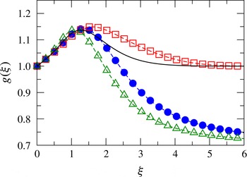
for the Oldroyd-B model. The circles correspond to the full Oldroyd-B solution of the FENE-P equations (2.28)–(2.30) for
 $P(R)=1$
; the squares correspond to the solution of the same equations neglecting the advection term in (2.29); the triangles correspond to the solution of the SPE model (2.33) and (2.34) with
 $\unicode[STIX]{x1D619}_{xy}=\langle l_{x}l_{y}\rangle$
; and the solid line corresponds to the solution of the SPE model with
 $\unicode[STIX]{x1D619}_{xy}$
computed using (2.36). Here,
 $Wi=1$
,
 $Re=4900$
and
 ${\it\gamma}=0.3$
.

We now review our approach for solving the problem with Oldroyd-B polymers in Benzi et al. (Reference Benzi, Ching and Chu2012) and explain why we adopt such an approach. For this purpose, we first solve the FENE-P equations (2.28)–(2.30) with
 $P(R)=1$
by assuming that
 ${\it\phi}({\it\xi})$
is given by the Blasius equation (2.9) without any feedback from the polymers. In other words, we consider the polymers to be passive. This (strong) approximation is made in the remainder of § 2.2 and in § 2.3 to illustrate the behaviour of the solution of the FENE-P equations. We show the normalized total effective viscosity
 $g({\it\xi})$
, defined as
 $$\begin{eqnarray}g({\it\xi})\equiv {\it\nu}_{tot}({\it\xi})/{\it\nu}_{0},\end{eqnarray}$$
so obtained as circles in figure 1. The parameters used are
 $Wi=1$
,
 $Re=4900$
and
 ${\it\gamma}=0.3$
, where
 $$\begin{eqnarray}{\it\gamma}\equiv \frac{{\it\nu}_{p}}{{\it\nu}_{0}}\end{eqnarray}$$
measures the fraction of the polymer contribution to the zero-shear viscosity of the solution and increases with the polymer concentration. We shall refer to this solution as the full Oldroyd-B solution. Oldroyd-B polymers are not shear thinning, so
 ${\it\nu}_{plate}={\it\nu}_{0}$
and
 $g(0)$
should be equal to
 $1$
. As shown in figure 1, this is found as expected. However, for large
 ${\it\xi}$
we observe that
 $g({\it\xi})$
goes to
 $0$
for
 ${\it\xi}\gg 1$
. This is clearly an unphysical result which does not match the expected zero-shear viscosity limit of
 $g({\it\xi})\rightarrow 1$
for large
 ${\it\xi}$
. The mathematical reason behind this unphysical result is due to the advection term in (2.29) for
 $\unicode[STIX]{x1D619}_{xy}$
. When we neglect this term, we obtain the result shown as squares in figure 1. As we can see, we are now able to recover the correct limit of the zero-shear viscosity at large
 ${\it\xi}$
. The bad news is, however, that the peak in
 $g({\it\xi})$
is shifted to a larger value of
 ${\it\xi}$
and it is wider. As we will show later in this paper, the position of the peak in
 $g({\it\xi})$
or its extension to the FENE-P model is crucial for understanding whether the resulting flow leads to heat reduction or heat enhancement. The position of the peak is mostly due to the advection terms in the FENE-P equations (2.28)–(2.30). The advection terms increase the stretching of the polymers because, very close to the boundary, they give a positive contribution to the conformational tensor. When we neglect the advection term in (2.29), we decrease the overall stretching of the polymers and shift the peak in
 $g({\it\xi})$
to a larger value of
 ${\it\xi}$
.
In order to make progress, we introduce a different approach, as described in our previous paper (Benzi et al.
Reference Benzi, Ching and Chu2012). We consider the equations for the normalized end-to-end distance vector,
 $\boldsymbol{l}\equiv \boldsymbol{d}/d_{0}$
, of a single polymer chain,
 $$\begin{eqnarray}\displaystyle & \displaystyle {\it\phi}\frac{\text{d}l_{x}}{\text{d}{\it\xi}}-\frac{1}{Wi}(l_{x}-l_{0x})-{\it\xi}{\it\phi}^{\prime \prime }l_{x}+2\sqrt{Re}\,{\it\phi}^{\prime \prime }l_{y}=0, & \displaystyle\end{eqnarray}$$
 $$\begin{eqnarray}\displaystyle & \displaystyle {\it\phi}\frac{\text{d}l_{y}}{\text{d}{\it\xi}}-\frac{1}{Wi}(l_{y}-l_{0y})-\frac{{\it\xi}^{2}{\it\phi}^{\prime \prime }}{2\sqrt{Re}}l_{x}+{\it\xi}{\it\phi}^{\prime \prime }l_{y}=0, & \displaystyle\end{eqnarray}$$
where
 $l_{0x}={\it\eta}_{x}l_{0}$
,
 $l_{0y}={\it\eta}_{y}l_{0}$
and
 $l_{0}^{2}=1$
. If we take
 $l_{0x}$
and
 $l_{0y}$
as white noise in
 ${\it\xi}$
, then using the standard tools of the stochastic differential equation (namely Ito calculus) we can derive the equation for the conformational tensor
 $\unicode[STIX]{x1D619}_{ij}=\overline{l_{i}l_{j}}$
, where
 $\overline{\cdots \,}$
stands for averaging over the noise. It is easy to show that, in this case, we recover the FENE-P equations (2.28)–(2.30) with
 $P(R)=1$
. Here, we consider (2.33) and (2.34) in a different way: we assume the polymer chain to have an equilibrium length
 $\sqrt{2}d_{0}$
, and
 ${\it\eta}_{x}$
and
 ${\it\eta}_{y}$
are random variables with
 $\langle {\it\eta}_{i}{\it\eta}_{j}\rangle ={\it\delta}_{ij}$
(to recover isotropy), where
 $\langle \cdots \rangle$
stands for averaging over the probability distribution of
 ${\it\eta}_{i}$
. For our purposes, we assume
 ${\it\eta}_{x}=\pm 1$
and
 ${\it\eta}_{y}=\pm 1$
with the same probability of
 $1/4$
. The basic idea is to compute the conformational tensor
 $\unicode[STIX]{x1D619}_{ij}$
, and in particular
 $\unicode[STIX]{x1D619}_{xy}$
needed for the computation of the effective viscosity, by using the single polymer equations (hereafter referred to as SPEs) (2.33) and (2.34) with
 $\unicode[STIX]{x1D619}_{ij}=\langle l_{i}l_{j}\rangle$
. In figure 1 we show
 $g({\it\xi})$
computed using the SPEs as triangles. It can be seen that this SPE solution is qualitatively and almost quantitatively similar to the full Oldroyd-B solution (circles), although the peak in
 $g({\it\xi})$
is now closer to the boundary. In fact, this SPE solution has the same flaw as the full Oldroyd-B solution, namely the limit of the zero-shear viscosity for large
 ${\it\xi}$
is not recovered. However, we can now make a crucial observation. We rewrite
 $\unicode[STIX]{x1D619}_{xy}$
as follows:
 $$\begin{eqnarray}\unicode[STIX]{x1D619}_{xy}=\langle l_{x}l_{y}\rangle =\langle (l_{x}-{\it\eta}_{x}l_{0})(l_{y}-{\it\eta}_{y}l_{0})\rangle +\langle l_{x}{\it\eta}_{y}\rangle l_{0}+\langle l_{y}{\it\eta}_{x}\rangle l_{0}.\end{eqnarray}$$
It should be noted that the term
 $\langle {\it\eta}_{x}{\it\eta}_{y}\rangle l_{0}^{2}=0$
and is thus dropped in (2.35). The first term on the right-hand side of (2.35) represents the effect of polymer stretching in
 $\unicode[STIX]{x1D619}_{xy}$
, and is zero both at the boundary and in the limit
 ${\it\xi}\gg 1$
. The second and third terms on the right-hand side of (2.35) are non-zero, and they are responsible for the behaviour of
 $\unicode[STIX]{x1D619}_{xy}$
at large
 ${\it\xi}$
. Therefore, the limit for large
 ${\it\xi}$
is controlled by
 ${\it\Delta}_{xy}\equiv \langle l_{x}{\it\eta}_{y}\rangle l_{0}+\langle l_{y}{\it\eta}_{x}\rangle l_{0}$
. The physical result of the zero-shear viscosity for large
 ${\it\xi}$
requires
 ${\it\Delta}_{xy}=Wi\sqrt{Re}\,{\it\phi}^{\prime \prime }$
. The above observations lead us to define (Benzi et al.
Reference Benzi, Ching and Chu2012) the value of
 $\unicode[STIX]{x1D619}_{xy}$
as
 $$\begin{eqnarray}\unicode[STIX]{x1D619}_{xy}=\langle (l_{x}-{\it\eta}_{x}l_{0})(l_{y}-{\it\eta}_{y}l_{0})\rangle +Wi\sqrt{Re}\,{\it\phi}^{\prime \prime }.\end{eqnarray}$$
The ansatz (2.36) is the main point under investigation in this subsection, and its generalization for the FENE-P model will be investigated next in § 2.3. In figure 1 we show
 $g({\it\xi})$
, computed using the SPEs and (2.36), as the solid line. As we can see,
 $g({\it\xi})$
is close to the full Oldroyd-B solution (circles) obtained using the FENE-P equations up to
 ${\it\xi}\sim 2$
and then smoothly recovers the limit of the zero-shear viscosity at large
 ${\it\xi}$
. It should be noted that the peak in
 $g({\it\xi})$
is now at the same position as that of the full Oldroyd-B solution, which means that the advection terms are correctly computed in the region close to the boundary. From a mathematical point of view, we can consider (2.36) as a simple way to filter advection terms for large
 ${\it\xi}$
, forcing the solution to satisfy the physical limit of the zero-shear viscosity. The quality of the results presented in figure 1 shows that this is a smart way to achieve the correct limit at large
 ${\it\xi}$
. To the best of our knowledge, there is no other simple way to achieve the same result starting from the full FENE-P equations.
2.3. Extension to the FENE-P model
The extension of the SPEs (2.33) and (2.34) for the FENE-P model is rather straightforward, namely we have
 $$\begin{eqnarray}\displaystyle & \displaystyle {\it\phi}\frac{\text{d}l_{x}}{\text{d}{\it\xi}}-\frac{1}{Wi}[P(R)l_{x}-l_{0x}]-{\it\xi}{\it\phi}^{\prime \prime }l_{x}+2\sqrt{Re}\,{\it\phi}^{\prime \prime }l_{y}=0, & \displaystyle\end{eqnarray}$$
 $$\begin{eqnarray}\displaystyle & \displaystyle {\it\phi}\frac{\text{d}l_{y}}{\text{d}{\it\xi}}-\frac{1}{Wi}[P(R)l_{y}-l_{0y}]-\frac{{\it\xi}^{2}{\it\phi}^{\prime \prime }}{2\sqrt{Re}}l_{x}+{\it\xi}{\it\phi}^{\prime \prime }l_{y}=0, & \displaystyle\end{eqnarray}$$
where the Peterlin function
 $P(R)$
is defined as in (2.14) with
 $R=\langle l_{x}^{2}\rangle +\langle l_{y}^{2}\rangle$
. In order to generalize the ansatz (2.36) to the FENE-P model, we need to consider the two limits
 ${\it\xi}=0$
and
 ${\it\xi}\gg 1$
. At large
 ${\it\xi}$
, the polymers do not stretch much so
 $P(R({\it\xi}))\rightarrow 1$
, and we expect
 ${\it\nu}_{tot}({\it\xi})\rightarrow {\it\nu}_{0}$
to recover the zero-shear viscosity limit for
 ${\it\xi}\gg 1$
. At the boundary, we can compute the value of
 $\unicode[STIX]{x1D619}_{xy}$
exactly using the FENE-P equations (2.28)–(2.30) and obtain
 $$\begin{eqnarray}{\it\nu}_{plate}={\it\nu}_{s}+\frac{{\it\nu}_{p}}{P_{0}},\end{eqnarray}$$
where
 $P_{0}\equiv P(R({\it\xi}=0))$
. We define the normalized total effective viscosity of the polymer solution by
 $$\begin{eqnarray}h({\it\xi})\equiv \frac{{\it\nu}_{tot}({\it\xi})}{{\it\nu}_{plate}},\end{eqnarray}$$
which is the extension of
 $g({\it\xi})$
to the FENE-P model, then we should have
 $$\begin{eqnarray}h(0)=1\end{eqnarray}$$
and expect
 $$\begin{eqnarray}h({\it\xi})\rightarrow \frac{{\it\nu}_{0}}{{\it\nu}_{plate}}=\frac{1}{1-{\it\gamma}+{\it\gamma}/P_{0}}\equiv h_{\infty },\quad {\it\xi}\gg 1.\end{eqnarray}$$
As
 $P_{0}>1$
, (2.42) tells us that
 $h(0)<h({\it\xi}\gg 1)$
, so the viscosity decreases when the shear is larger near the boundary, thus the FENE-P polymer flow is shear thinning. The model now depends on three parameters, namely the Weissenberg number
 $Wi$
,
 ${\it\gamma}$
measuring the polymer concentration as for the Oldroyd-B model and
 $b^{2}$
measuring the finite extensibility of the FENE-P polymers. For very large
 $b^{2}$
we do not expect any difference with respect to the Oldroyd-B case.
We take the reference viscosity
 ${\it\nu}_{r}$
to be the viscosity of the polymer solution at the plate,
 ${\it\nu}_{plate}$
, in (2.23) and (2.25) and obtain
 $$\begin{eqnarray}{\textstyle \frac{1}{2}}{\it\phi}{\it\phi}^{\prime \prime }+(h{\it\phi}^{\prime \prime })^{\prime }=0,\end{eqnarray}$$
with
 $$\begin{eqnarray}h({\it\xi})=h_{\infty }\left[(1-{\it\gamma})+\frac{{\it\gamma}}{Wi\sqrt{Re}\,{\it\phi}^{\prime \prime }}P\unicode[STIX]{x1D619}_{xy}\right].\end{eqnarray}$$
Equation (2.44) suggests that the generalization of the ansatz (2.36) to the FENE-P model is given by
 $$\begin{eqnarray}\unicode[STIX]{x1D619}_{xy}=\frac{\langle [P(R)l_{x}-{\it\eta}_{x}l_{0}][P(R)l_{y}-{\it\eta}_{y}l_{0}]\rangle +Wi\sqrt{Re}\,{\it\phi}^{\prime \prime }}{[P(R)]^{2}},\end{eqnarray}$$
which meets both the requirement (2.41) and the zero-shear viscosity limit (2.42). It remains to understand whether the ansatz (2.45) properly represents the physics of the FENE-P model.
Mathematically, we cannot expect
 $\unicode[STIX]{x1D619}_{xy}$
computed from the SPEs (2.37) and (2.38) using the ansatz (2.45) to match the one computed from the FENE-P equations (2.28)–(2.30) near the boundary for exactly the same values of
 $b^{2}$
and
 ${\it\gamma}$
. As we shall explain at the end of § 3, the effect of
 $b^{2}$
is to shift the peak in
 $h({\it\xi})$
towards larger values of
 ${\it\xi}$
as
 $b^{2}$
decreases, and such a shift is not the same for the two models under consideration. Moreover, it is crucial to require the same effective viscosity at the boundary. Therefore, if our model makes sense, we expect to achieve agreement between the two models for different values of
 $b^{2}$
and
 ${\it\gamma}$
, although such differences (if any) should be small.
(a) The normalized total effective viscosity
 $h({\it\xi})={\it\nu}_{tot}({\it\xi})/{\it\nu}_{plate}$
and (b) the Peterlin function
 $P(R({\it\xi}))$
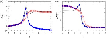
for the FENE-P model. The circles correspond to the full solution of the FENE-P equations (2.28)–(2.30); the squares correspond to the solution of the same equations neglecting the advection term in (2.29); the solid line corresponds to the solution of the SPE model with
 $\unicode[STIX]{x1D619}_{xy}$
computed using (2.45). For the FENE-P equations with and without the advection term,
 $b^{2}=50$
and
 ${\it\gamma}=0.3$
, while for the SPE model,
 $b^{2}=60$
and
 ${\it\gamma}=0.33$
;
 $Wi=2$
in both cases.

In figure 2(a), we show
 $h({\it\xi})$
for
 $Wi=2$
calculated using the FENE-P equations, with and without the advection term in (2.29), with the parameters
 $(b^{2}=50,{\it\gamma}=0.3)$
, and using the SPEs supplemented with (2.45), with the parameters
 $(b^{2}=60,{\it\gamma}=0.33)$
. In figure 2(b), we show the function
 $P(R)$
calculated in the three ways. The symbols are the same as in figure 1: the circles are the full solution of the FENE-P equations, the squares are the solution of the FENE-P equations without the advection term in the
 $\unicode[STIX]{x1D619}_{xy}$
equation and finally the solid line is the solution of the SPE model solving (2.37) and (2.38) with (2.45). We start by highlighting three major points in figure 2(b): the value of
 $P_{0}$
is different for the full solution of the FENE-P model and the SPE model; the peak in
 $P(R)$
observed in the full solution of the FENE-P model is also obtained quite accurately for the SPE model; finally, the solution of the FENE-P equations without the advection term in the
 $\unicode[STIX]{x1D619}_{xy}$
equation completely misses the peak in
 $P(R)$
. Let us remark that these particular results are independent of the ansatz (2.45). The above observations indicate one negative point about the SPE model, in that it underestimates the value of
 $P(R)$
at the boundary. This is the reason why we need to use a different value of
 ${\it\gamma}$
in the SPE model. In fact, using (2.45) and a slightly different value of
 ${\it\gamma}$
, we achieve the same effective viscosity at the boundary as shown in figure 2(a). The (very) good news is that both the position and the amplitude of the peak in
 $P(R)$
and
 $h({\it\xi})$
obtained using the full FENE-P equations (circles) and our approach using the SPEs with the definition (2.45) of
 $\unicode[STIX]{x1D619}_{xy}$
(solid line) are in agreement with one another. Thus, as long as we are mostly interested in computing the effective viscosity, our approach is extremely efficient in computing
 $h({\it\xi})$
with the correct asymptotic limits and taking into account the effect of stretching near the boundary.
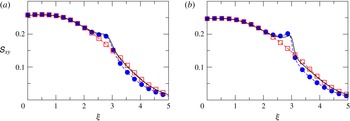
The validity of the ansatz (2.45) is investigated in figure 3. From (2.43), we see that
 $h({\it\xi}){\it\phi}^{\prime \prime }$
corresponds to the full momentum stress due to viscous and polymeric effects. We consider the quantity
 $$\begin{eqnarray}\unicode[STIX]{x1D61A}_{xy}\equiv \frac{h({\it\xi}){\it\phi}^{\prime \prime }}{h_{\infty }}=\left[(1-{\it\gamma}){\it\phi}^{\prime \prime }+\frac{{\it\gamma}}{Wi\sqrt{Re}}P\unicode[STIX]{x1D619}_{xy}\right].\end{eqnarray}$$
In figure 3(a), we show the behaviour of
 $\unicode[STIX]{x1D61A}_{xy}$
for the same case at
 $Wi=2$
previously discussed in figure 2, while in figure 3(b), we consider the case
 $Wi=5$
and
 $(b^{2}=50,{\it\gamma}=0.3)$
for the FENE-P equations with and without the advection term in (2.29) and
 $(b^{2}=50,{\it\gamma}=0.32)$
for the SPE model. For both values of
 $Wi$
, we observe a clear and non-trivial agreement between the full solution of the FENE-P equations and our approach up to the point where
 $\unicode[STIX]{x1D61A}_{xy}\leqslant {\it\phi}^{\prime \prime }$
.


To summarize the results discussed in this subsection, we have shown that the original FENE-P equations cannot be used in the framework of the Prandtl–Blasius boundary layer theory in a straightforward way because they lead to unphysical results. Our approach retains the physics of the FENE-P model without the unphysical drawbacks in the effective viscosity. The quality of the results shown in figures 2 and 3 verifies the validity of our model, which, to the best of our knowledge, is the only way to understand polymer dynamics within the framework of the Prandtl–Blasius boundary layer theory.
2.4. Comparison of heat transport
A trivial effect of adding polymers to a Newtonian fluid is that the zero-shear viscosity increases. Even for a Newtonian fluid with Prandtl number greater than 1, an increase in the viscosity leads to a reduction in
 $Nu$
. Thus, to focus on the effect on heat transport due to the non-Newtonian nature of the polymers and not the mere increase of the viscosity, we compare the value of
 $Nu$
in the presence of polymers to the reference value
 $Nu_{0}$
for a Newtonian fluid with a kinematic viscosity
 ${\it\nu}$
equal to that of the polymer solution at the plate, namely
 ${\it\nu}={\it\nu}_{plate}$
. To find
 $Nu$
in the presence of polymers, we solve the SPE model (2.37) and (2.38) with (2.45) and (2.43) with (2.44). These equations are coupled as the polymers are active. We use an iterative scheme devised in Benzi et al. (Reference Benzi, Ching and Chu2012). We start to calculate
 $\unicode[STIX]{x1D619}_{xy}$
and thus
 $h({\it\xi})$
by solving the SPE model with
 ${\it\phi}({\it\xi})$
taken to be the Blasius solution without polymers governed by (2.9), denoted as
 ${\it\phi}_{B}$
. Using this calculated
 $h({\it\xi})$
, we solve (2.43) to obtain an updated
 ${\it\phi}({\it\xi})$
. With this updated
 ${\it\phi}({\it\xi})$
, we repeat the procedure until both
 $h({\it\xi})$
and
 ${\it\phi}({\it\xi})$
converge. Using this convergent solution of
 ${\it\phi}({\it\xi})$
, we solve the temperature equation (2.8) with
 ${\it\nu}_{r}={\it\nu}_{plate}$
to obtain
 ${\it\theta}({\it\xi})$
and thus
 $Nu$
by
 $$\begin{eqnarray}Nu=\sqrt{\frac{UL}{{\it\nu}_{plate}}}[-{\it\theta}^{\prime }(0)].\end{eqnarray}$$
That is,
 ${\it\theta}({\it\xi})$
satisfies the equation
 $$\begin{eqnarray}2{\it\theta}^{\prime \prime }+\left(\frac{{\it\nu}_{plate}}{{\it\nu}_{s}}\right)Pr_{s}\,{\it\phi}{\it\theta}^{\prime }=0,\end{eqnarray}$$
where
 $Pr_{s}\equiv {\it\nu}_{s}/{\it\kappa}$
is the Prandtl number of the Newtonian fluid before polymers are added. To obtain the reference value of
 $Nu_{0}$
for a Newtonian fluid with a kinematic viscosity
 ${\it\nu}_{plate}$
, the same as that of the polymer solution at the plate, we solve (2.7) and (2.8) with
 ${\it\phi}={\it\phi}_{B}$
and
 ${\it\nu}={\it\nu}_{r}={\it\nu}_{plate}$
, and thus obtain
 $$\begin{eqnarray}Nu_{0}=\sqrt{\frac{UL}{{\it\nu}_{plate}}}[-{\it\theta}_{B}^{\prime }(0)],\end{eqnarray}$$
where
 ${\it\theta}_{B}({\it\xi})$
satisfies (2.48) with
 ${\it\phi}({\it\xi})={\it\phi}_{B}({\it\xi})$
, namely
 $$\begin{eqnarray}2{\it\theta}_{B}^{\prime \prime }+\left(\frac{{\it\nu}_{plate}}{{\it\nu}_{s}}\right)Pr_{s}\,{\it\phi}_{B}{\it\theta}_{B}^{\prime }=0.\end{eqnarray}$$
We are interested in studying the ratio
 $$\begin{eqnarray}\frac{Nu}{Nu_{0}}=\frac{{\it\theta}^{\prime }(0)}{{\it\theta}_{B}^{\prime }(0)}.\end{eqnarray}$$
In experimental studies, it is common to directly compare the value of
 $Nu$
in the presence of polymers with the value
 $Nu_{s}$
of the Newtonian fluid before polymers are added. To calculate
 $Nu_{s}$
, we solve (2.7) and (2.8) with
 ${\it\phi}={\it\phi}_{B}$
and take both
 ${\it\nu}$
and
 ${\it\nu}_{r}$
to be
 ${\it\nu}_{s}$
, the kinematic viscosity of the Newtonian fluid before polymers are added. In this case, the temperature, denoted as
 ${\it\theta}_{s}$
, satisfies the equation
 $$\begin{eqnarray}2{\it\theta}_{s}^{\prime \prime }+Pr_{s}\,{\it\phi}_{B}{\it\theta}_{s}^{\prime }=0,\end{eqnarray}$$
and we obtain
 $$\begin{eqnarray}Nu_{s}=\sqrt{\frac{UL}{{\it\nu}_{s}}}[-{\it\theta}_{s}^{\prime }(0)].\end{eqnarray}$$
It should be noted that
 ${\it\theta}_{B}({\it\xi})$
and
 ${\it\theta}_{s}({\it\xi})$
are solutions to the same temperature equation (2.8) with
 ${\it\phi}={\it\phi}_{B}$
but with different Prandtl numbers,
 $Pr_{s}({\it\nu}_{plate}/{\it\nu}_{s})$
and
 $Pr_{s}$
(cf. (2.50) and (2.52)). For large
 $Pr_{s}$
(
 ${>}$
1),
 ${\it\phi}_{B}({\it\xi})$
can be approximated as
 ${\it\phi}_{B}^{\prime \prime }(0){\it\xi}^{2}/2$
when solving (2.52), and this leads to
 $|{\it\theta}_{s}^{\prime }(0)|\propto Pr_{s}^{1/3}$
(Schlichting & Gersten Reference Schlichting and Gersten2004). Thus,
 ${\it\theta}_{B}^{\prime }(0)/{\it\theta}_{s}^{\prime }(0)\approx ({\it\nu}_{plate}/{\it\nu}_{s})^{1/3}$
, and (2.49) and (2.53) imply
 $Nu_{0}/Nu_{s}\approx ({\it\nu}_{s}/{\it\nu}_{plate})^{1/6}$
. From (2.39),
 ${\it\nu}_{s}<{\it\nu}_{plate}$
; therefore, we have
 $Nu/Nu_{s}<Nu/Nu_{0}$
.
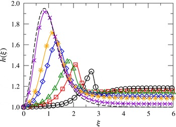
The normalized total effective viscosity profile
 $h({\it\xi})$
for
 $b^{2}=100$
(circles),
 $b^{2}=500$
(squares),
 $b^{2}=1000$
(triangles),
 $b^{2}=5000$
(diamonds),
 $b^{2}=10^{4}$
(stars),
 $b^{2}=10^{5}$
(crosses) and
 $1/b=0$
(dashed line) for
 $Wi=5.0$
and
 ${\it\gamma}=0.2$
.

3. Results and discussion
3.1. Dependence of heat transport on the parameters
We study the dependence of
 $Nu/Nu_{0}$
on the three parameters:
 $b^{2}$
measuring the finite extensibility of the polymers,
 $Wi$
measuring the polymer relaxation time and
 ${\it\gamma}$
measuring the polymer concentration for fixed Prandtl and Reynolds numbers,
 $Pr_{s}\equiv {\it\nu}_{s}/{\it\kappa}Re_{s}\equiv UL/{\it\nu}_{s}$
, of the Newtonian fluid before polymers are added. The results presented in this paper are obtained using
 $Pr_{s}=4.4$
and
 $Re_{s}=4900$
. This value of
 $Pr_{s}$
corresponds to that of water at approximately 40
 $^{\circ }$
C. To connect to turbulent RB convection,
 $Re_{s}$
plays the role of the Reynolds number
 $Re$
of the large-scale mean flow, which is related to the Rayleigh number
 $Ra$
by
 $Re=0.085Ra^{0.455}$
for water at moderate
 $Ra$
(Grossmann & Lohse Reference Grossmann and Lohse2002); thus,
 $Re_{s}=4900$
corresponds to
 $Ra\sim 10^{10}$
. These values of
 $Pr_{s}$
and
 $Re_{s}$
are chosen to be close to those in the experimental studies (Ahlers & Nikolaenko Reference Ahlers and Nikolaenko2010; Wei, Ni & Xia Reference Wei, Ni and Xia2012).
We first study the profile of the normalized total effective viscosity
 $h({\it\xi})$
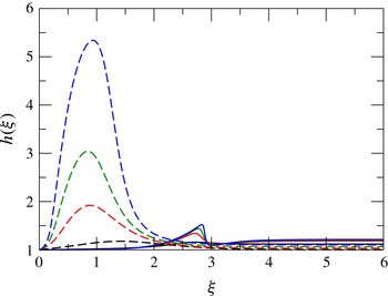
of the polymer solution. In figure 4, we show
 $h({\it\xi})$
for different values of
 $b^{2}$
for
 $Wi=5$
and
 ${\it\gamma}=0.2$
. It can be seen that
 $h({\it\xi})$
increases from 1 at the boundary, cf. (2.41), attaining a maximum value
 $h_{m}\equiv h({\it\xi}_{p})$
at some position
 ${\it\xi}_{p}$
, and then approaches the asymptotic value
 $h_{\infty }$
, satisfying the zero-shear viscosity limit as
 ${\it\xi}\rightarrow \infty$
. When
 $b^{2}$
decreases, the amount of polymer stretching decreases, but the polymer chain can be stretched closer to the maximum allowed value, such that
 $P_{0}$
is larger; thus, we expect
 $h_{m}$
to decrease but
 $h_{\infty }$
to increase. As can be seen in figure 4, these features are found as expected. We see also that the peak position
 ${\it\xi}_{p}$
moves away from the plate when
 $b^{2}$
decreases. We shall explain this behaviour near the end of this section.
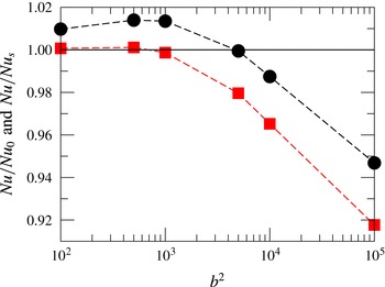
In figure 5, we compare the
 $Nu$
of the polymer solution with the reference value
 $Nu_{0}$
of a Newtonian fluid with a kinematic viscosity
 ${\it\nu}_{plate}$
as well as with
 $Nu_{s}$
of the Newtonian fluid before polymers are added for the cases shown in figure 4. It can be seen that the nature of heat transport modification depends on the value of
 $b^{2}$
. For very large
 $b^{2}$
, heat transport is reduced, as found for Oldroyd-B polymers in our previous work (Benzi et al.
Reference Benzi, Ching and Chu2012). For small
 $b^{2}$
(smaller than approximately 5000),
 $Nu/Nu_{0}>1$
. For even smaller
 $b^{2}$
(smaller than approximately 1000),
 $Nu/Nu_{s}$
is also larger than 1. Hence, there is a transition from heat reduction to heat enhancement when
 $b^{2}$
is decreased.
The dependence of
 $Nu/Nu_{0}$
(circles) and
 $Nu/Nu_{s}$
(squares) on
 $b^{2}$
for
 $Wi=5$
and
 ${\it\gamma}=0.2$
. Here,
 $Nu_{0}$
is the reference value obtained for a Newtonian fluid of kinematic viscosity
 ${\it\nu}_{plate}$
, the same as that of the polymer solution at the plate, while
 $Nu_{s}$
is the Nusselt number for the Newtonian fluid before polymers are added.

Next, we investigate this transition as a function of
 $Wi$
and
 ${\it\gamma}$
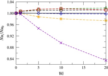
. We first show the dependence of
 $Nu/Nu_{0}$
on
 $Wi$
at
 ${\it\gamma}=0.2$
in figure 6. We find heat reduction for large
 $b^{2}$
and heat enhancement for small
 $b^{2}$
for all of the values of
 $Wi$
studied. The amount of heat reduction increases with
 $Wi$
, as found previously for Oldroyd-B polymers (Benzi et al.
Reference Benzi, Ching and Chu2012). On the other hand, the amount of heat enhancement increases slightly with
 $Wi$
for small
 $Wi$
, and becomes almost independent of
 $Wi$
for larger
 $Wi$
.
The dependence of
 $Nu/Nu_{0}$
on
 $Wi$
at
 ${\it\gamma}=0.2$
for
 $b^{2}=100$
, 500, 1000, 5000,
 $10^{4}$
and
 $10^{5}$
. The symbols are the same as in figure 4.

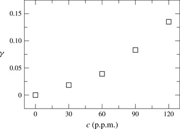
The dependence of
 ${\it\gamma}$
on the concentration
 $c$
for a polymer solution of PEO with a nominal molecular weight of
 $4\times 10^{6}~\text{g}~\text{mol}^{-1}$
, obtained by using the experimental measurements in Wei, Ni & Xia (Reference Wei, Ni and Xia2012).

Next, we study how
 $Nu/Nu_{0}$
depends on
 ${\it\gamma}$
at a fixed value of
 $Wi$
. The parameter
 ${\it\gamma}$
is a measure of the polymer concentration. Using experimental measurements of the kinematic viscosity of the polymer solution
 ${\it\nu}_{sol}(c)$
for different polymer concentrations
 $c$
, the dependence of
 ${\it\gamma}$
on
 $c$
can be obtained. We take the polymer PEO (polyethylene oxide) as an example. Since PEO is a highly flexible polymer,
 $b^{2}$
is very large and the shear-thinning effect is negligible. Thus,
 ${\it\nu}_{sol}(c)$
is given by the zero-shear viscosity
 ${\it\nu}_{0}$
, and
 ${\it\nu}_{sol}(c)/{\it\nu}_{s}=1/(1-{\it\gamma})$
. Using the experimental measurements from Wei, Ni & Xia (Reference Wei, Ni and Xia2012), we calculate
 ${\it\gamma}$
as a function of
 $c$
and show the results in figure 7. It can be seen that
 ${\it\gamma}$
increases with
 $c$
. As we are interested in polymer concentrations of the order of a few hundreds of p.p.m. like those used in the experiments, we focus on
 $0\leqslant {\it\gamma}\leqslant 0.4$
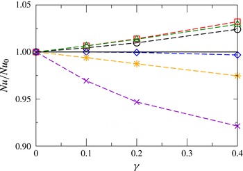
. The dependence of
 $Nu/Nu_{0}$
on
 ${\it\gamma}$
for
 $Wi=5$
is shown in figure 8. Again, we see that
 $Nu/Nu_{0}<1$
for very large
 $b^{2}$
and
 $Nu/Nu_{0}>1$
for small
 $b^{2}$
. In Benzi et al. (Reference Benzi, Ching and Chu2012), we show that the amount of heat reduction increases with
 ${\it\gamma}$
for Oldroyd-B polymers. As can be seen in figure 8, we find similar results for FENE-P polymers, namely the amount of heat reduction or enhancement increases with
 ${\it\gamma}$
. Combining the results shown in figures 6 and 8, we see that the nature of heat transport modification depends only on the parameter
 $b^{2}$
: heat transport is reduced for very large
 $b^{2}$
and enhanced for small
 $b^{2}$
, and this is true for the values of
 $Wi$
and
 ${\it\gamma}$
(
 $0<Wi\leqslant 20$
and
 $0<{\it\gamma}\leqslant 0.4$
) studied.


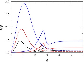
The profile
 $h({\it\xi})$
for different values of
 $Wi$
(
 $Wi=1,5,10,20$
from bottom to top) for
 $b^{2}=100$
(solid lines) and
 $b^{2}=10\,000$
(dashed lines) at
 ${\it\gamma}=0.2$
.

The profile
 $h({\it\xi})$
for different values of
 ${\it\gamma}$
(
 ${\it\gamma}=0.1,0.2,0.4$
from bottom to top) for
 $b^{2}=100$
(solid lines) and
 $b^{2}=10\,000$
(dashed lines) at
 $Wi=5$
.

3.2. Understanding the results using a model of
 $h({\it\xi})$

Our results show that there is a transition from heat reduction to heat enhancement when
 $b^{2}$
is decreased. We now discuss how the transition can be explained in terms of the functional shape of the effective viscosity
 $h({\it\xi})$
. As seen in figure 4, the profile of
 $h({\it\xi})$
is described by three key features, namely the peak position
 ${\it\xi}_{p}$
, the peak value
 $h_{m}$
and the asymptotic value
 $h_{\infty }$
. When
 $b^{2}$
is decreased at fixed
 $Wi$
and
 ${\it\gamma}$
, the peak position
 ${\it\xi}_{p}$
moves away from the boundary, the peak value
 $h_{m}$
decreases and
 $h_{\infty }$
increases. In figure 9, we show how the profiles of
 $h({\it\xi})$
for
 $b^{2}=100$
and
 $100\,000$
vary as
 $Wi$
is changed for
 ${\it\gamma}=0.2$
. The dependence of the profiles of
 $h({\it\xi})$
on
 ${\it\gamma}$
at
 $Wi=5$
for the same two values of
 $b^{2}$
is shown in figure 10. From figures 9 and 10, we see clearly that while both the peak value
 $h_{m}$
and the asymptotic value
 $h_{\infty }$
increase with
 $Wi$
or
 ${\it\gamma}$
, the peak position
 ${\it\xi}_{p}$
remains almost unchanged for the same
 $b^{2}$
. Thus, we observe a common characteristic: the transition from heat reduction to heat enhancement is accompanied by an increase in
 ${\it\xi}_{p}$
or the moving away of the peak position of
 $h({\it\xi})$
from the plate. This observation suggests that heat transport is enhanced when the peak position
 ${\it\xi}_{p}$
is sufficiently far away from the plate. A physically relevant length scale would be the thermal boundary layer thickness. Thus, we have an interesting prediction: heat transport is enhanced when the peak position
 ${\it\xi}_{p}$
moves outside the thermal boundary layer.
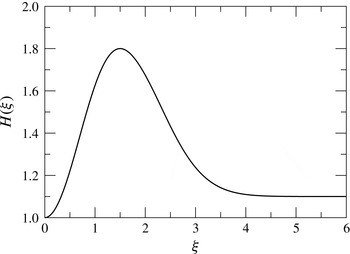
An example of the model effective viscosity
 $H({\it\xi})$
, calculated using (A 1), with
 ${\it\xi}_{p}=1.5$
,
 $H_{m}=1.8$
and
 $H_{\infty }=1.1$
.

To check our prediction, we model
 $h({\it\xi})$
by an analytical mathematical form discussed in appendix A, see (A 1), denoted as
 $H({\it\xi})$
, which has three parameters describing the same three key features: a peak at
 ${\it\xi}_{p}$
with the peak value
 $H_{m}$
and an asymptotic value of
 $H_{\infty }$
as
 ${\it\xi}\rightarrow \infty$
. An example of the model effective viscosity
 $H({\it\xi})$
with
 ${\it\xi}_{p}=1.5$
,
 $H_{m}=1.8$
and
 $H_{\infty }=1.1$
is shown in figure 11. The use of
 $H({\it\xi})$
allows us to study the effect of each of the three features separately. We solve (2.43) with
 $h({\it\xi})$
replaced by this model effective viscosity
 $H({\it\xi})$
and (2.8) (with
 ${\it\nu}_{r}={\it\nu}_{s}$
) and compare
 $Nu$
so obtained with the value
 $Nu_{ref}$
obtained using
 $H=1$
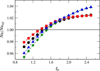
. In figure 12, we show
 $Nu/Nu_{ref}$
as a function of
 ${\it\xi}_{p}$
for different values of
 $H_{m}$
and
 $H_{\infty }$
. It can be seen that there is a transition from heat reduction to heat enhancement whenever
 ${\it\xi}_{p}$
is larger than some critical value
 ${\it\xi}_{c}$
for all of the cases studied. The value of
 ${\it\xi}_{c}$
depends weakly on
 $H_{m}$
and
 $H_{\infty }$
. The dimensionless thermal boundary layer thickness is defined by
 $$\begin{eqnarray}{\it\delta}_{T}=\frac{1}{|{\it\theta}^{\prime }(0)|},\end{eqnarray}$$
and decreases with
 $Pr_{s}$
. We change
 $Pr_{s}$
and study how
 ${\it\xi}_{c}$
depends on
 ${\it\delta}_{T}$
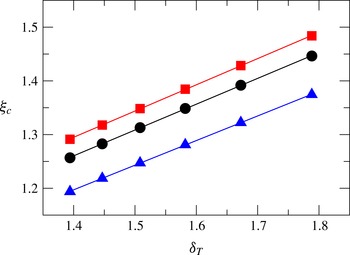
. As shown in figure 13,
 ${\it\xi}_{c}$
increases linearly with
 ${\it\delta}_{T}$
and is of the order of
 ${\it\delta}_{T}$
. These results confirm our prediction that heat transport is enhanced when the peak position or the region of polymer stretching goes beyond the thermal boundary layer.
Finally, we explain the dependence of the peak position
 ${\it\xi}_{p}$
of
 $h({\it\xi})$
on
 $b^{2}$
in the limit of small
 $Wi$
and
 ${\it\gamma}$
. In this limit, to a first-order approximation (2.44) is given by
 $$\begin{eqnarray}h({\it\xi})\approx 1+\frac{{\it\gamma}}{b^{2}R_{0}}[R(0)-R({\it\xi})],\end{eqnarray}$$
where we have used
 $b^{2}-1\approx b^{2}$
. Then, (2.43) becomes
 $$\begin{eqnarray}\frac{1}{2}{\it\phi}{\it\phi}^{\prime \prime }-\frac{{\it\gamma}}{b^{2}R_{0}}(R)^{\prime }{\it\phi}^{\prime \prime }+\left\{1+\frac{{\it\gamma}}{b^{2}R_{0}}[R(0)-R]\right\}{\it\phi}^{\prime \prime \prime }=0.\end{eqnarray}$$
For
 ${\it\gamma}=0$
, (3.3) reduces to the Blasius equation (2.9), which is invariant upon the scale transformation of
 ${\it\xi}\rightarrow {\it\lambda}{\it\xi}$
and
 ${\it\phi}\rightarrow {\it\lambda}^{-1}{\it\phi}$
. For
 ${\it\gamma}\neq 0$
, (3.3) is invariant under the same transformation together with
 ${\it\gamma}/b^{2}\rightarrow {\it\lambda}{\it\gamma}/b^{2}$
and
 $R({\it\xi})\rightarrow {\it\lambda}^{-1}R({\it\xi})$
. This implies
 $h^{\prime }={\it\gamma}/(b^{2}R_{0})(R)^{\prime }\rightarrow {\it\lambda}^{-1}h^{\prime }$
. Thus, when
 $b^{2}$
is decreased, which is equivalent to increasing
 ${\it\lambda}$
,
 $h^{\prime }\sim {\it\lambda}^{-1}$
decreases. As a result, the peak position moves away from the plate when
 $b^{2}$
is decreased. This explains our observations discussed earlier.
Comparison of
 $Nu$
using the model effective viscosity
 $H({\it\xi})$
with parameters
 ${\it\xi}_{p}$
,
 $H_{m}$
and
 $H_{\infty }$
with the value
 $Nu_{ref}$
obtained for
 $H=1$
. The value of
 $Pr_{s}$
is
 $4.5$
. The circles are results for
 $H_{m}=1.6$
and
 $H_{\infty }=1.1$
, the squares are results for
 $H_{m}=1.6$
and
 $H_{\infty }=1.2$
, the diamonds are results for
 $H_{m}=2.0$
and
 $H_{\infty }=1.1$
, and the triangles are results for
 $H_{m}=2.0$
and
 $H_{\infty }=1.2$
.

The dependence of
 ${\it\xi}_{c}$
on the dimensionless thermal boundary layer thickness
 ${\it\delta}_{T}$
as
 $Pr_{s}$
is varied from
 $4.5$
to
 $9.5$
for
 $H_{m}=1.4$
and
 $H_{\infty }=1.05$
(circles),
 $H_{m}=1.6$
and
 $H_{\infty }=1.05$
(squares), and
 $H_{m}=1.6$
and
 $H_{\infty }=1.2$
(triangles).

4. Summary and conclusions
We have studied the effect of finitely extensible polymers, described by the FENE-P model, on heat transport within the framework of the Prandtl–Blasius–Pohlhausen boundary layer theory. In the FENE-P model, the finite extensibility of polymers is measured by the parameter
 $b^{2}$
, which is the ratio of the maximum to the equilibrium value of the trace of the polymer conformation tensor. We have shown that we should keep only the shear stress
 $\unicode[STIX]{x1D61B}_{xy}$
of the polymer stress tensor and discard the normal stress
 $\unicode[STIX]{x1D61B}_{xx}$
in order to avoid the unphysical result of an infinite viscosity due to polymers far away from the boundary. Then, the polymer shear stress, which is proportional to
 $\unicode[STIX]{x1D619}_{xy}$
of the polymer conformation tensor, gives rise to a position-dependent effective viscosity. We have explained that the equations for the conformation tensor (2.28)–(2.30) in the FENE-P model cannot be used directly because they lead to unphysical results in that the zero-shear viscosity cannot be recovered far away from the boundary. We have introduced another approach by studying the SPEs (2.33) and (2.34) together with the definition (2.45) for
 $\unicode[STIX]{x1D619}_{xy}$
. We have demonstrated that our approach retains the physics of the FENE-P model without the unphysical drawback in the effective viscosity. To the best of our knowledge, our approach is the only way to understand polymer dynamics within the framework of the Prandtl–Blasius boundary layer theory. Using our approach, we have calculated
 $\unicode[STIX]{x1D619}_{xy}$
and studied how heat transport is affected. Heat transport is reduced for very large
 $b^{2}$
, as found in our previous study (Benzi et al.
Reference Benzi, Ching and Chu2012) of Oldroyd-B polymers, which can be extended indefinitely with
 $b\rightarrow \infty$
. The new finding in the present work is that there is a transition to heat transport enhancement when
 $b^{2}$
is small. We have further shown that this transition from heat reduction to heat enhancement can be explained in terms of the functional shape of the space-dependent effective viscosity due to the polymers. Heat transport is enhanced when the peak position of the effective viscosity profile or the region of substantial polymer stretching moves outside the thermal boundary layer. As
 $b^{2}$
is decreased, the peak position moves away from the plate and beyond the thermal boundary layer, thus giving rise to the transition.
Measurements of heat transfer were carried out for laminar flow of dilute PEO polymer solution around heated cylinders, and a reduction in heat transfer was reported (James & Acosta Reference James and Acosta1970). Polyethylene oxide is a highly flexible polymer, and is thus described by the FENE-P model with a very large
 $b^{2}$
. This experimental finding is, therefore, consistent with our result of heat reduction for very large
 $b^{2}$
. There is no systematic experimental study on the effect of the finite extensibility of polymers in the literature, except that an enhancement in heat transport has been reported for shear-thinning fluid over a heated cylinder (Mizushina et al.
Reference Mizushina, Usui, Veno and Kato1978; Khan, Culham & Yovanovich Reference Khan, Culham and Yovanovich2006; Delouei et al.
Reference Delouei, Nazari, Kayhani and Succi2014). Shear-thinning fluid can be described by the FENE-P model, and the larger the shear-thinning effect, the smaller the value of
 $b^{2}$
is. The above experimental finding is thus consistent with our result of heat enhancement for small
 $b^{2}$
.
We end our paper by discussing how our results allow us to gain an understanding of the experimental results in turbulent RB convection with polymers. In experiments (Ahlers & Nikolaenko Reference Ahlers and Nikolaenko2010; Wei, Ni & Xia Reference Wei, Ni and Xia2012) in a convection cell with the usual smooth top and bottom plates, the thermal boundary layer thickness is rather large for the range of moderate
 $Ra$
studied. Thus, the region of substantial polymer stretching remains close to the boundary even when the polymer concentration is increased, which implies, as observed experimentally, heat transport reduction. In this case, increasing the polymer concentration would increase the amount of heat reduction, again as observed experimentally. On the other hand, for experiments performed in a convection cell with rough top and bottom plates, the rough surfaces would disturb the thermal boundary layers and reduce their thickness significantly. Thus, it is possible that polymers can stretch outside the thermal boundary layers, most likely when the polymer concentration increases. When this happens, there would be a transition from heat reduction to heat enhancement as the polymer concentration is increased, and this was indeed observed in experiments (Wei, Ni & Xia Reference Wei, Ni and Xia2012).
Acknowledgements
R.B. acknowledges the support of project RITMARE, and the work of E.S.C.C., W.C.K.Y. and Y.W. was supported by the Hong Kong Research Grants Council under grant no. CUHK-400311.
Appendix A. Mathematical expression of the model effective viscosity
The mathematical expression of the model effective viscosity
 $H({\it\xi})$
is given by
 $$\begin{eqnarray}H({\it\xi})=g_{0}\left(\frac{{\it\xi}}{{\it\xi}_{0}}\right)^{2}\exp \left[1-\left(\frac{{\it\xi}}{{\it\xi}_{0}}\right)^{2}\right]+\frac{(H_{\infty }-1)}{2}\tanh (2{\it\xi}-4)+\frac{(H_{\infty }+1)}{2}.\end{eqnarray}$$
At
 ${\it\xi}=0$
,
 $H(0)\approx 1$
, and
 $H({\it\xi})\rightarrow H_{\infty }$
as
 ${\it\xi}\rightarrow \infty$
. Moreover,
 $H({\it\xi})$
peaks at
 ${\it\xi}_{p}$
with the value
 $H_{m}$
. The parameters
 ${\it\xi}_{0}$
and
 $g_{0}$
are related to
 ${\it\xi}_{p}$
,
 $H_{m}$
and
 $H_{\infty }$
by
 $$\begin{eqnarray}\displaystyle & \displaystyle {\it\xi}_{0}=\sqrt{\frac{K}{{\it\xi}_{p}+K}}{\it\xi}_{p}, & \displaystyle\end{eqnarray}$$
 $$\begin{eqnarray}\displaystyle & \displaystyle g_{0}=K\frac{(H_{\infty }-1)}{2}\left(\frac{{\it\xi}_{p}}{{\it\xi}_{0}}\right)^{-2}\exp \left[\left(\frac{{\it\xi}_{p}}{{\it\xi}_{0}}\right)^{2}-1\right]\cosh ^{-2}(2{\it\xi}_{p}-4), & \displaystyle\end{eqnarray}$$
with
 $$\begin{eqnarray}K=\left[\frac{2H_{m}-H_{\infty }-1}{H_{\infty }-1}-\tanh (2{\it\xi}_{p}-4)\right]\cosh ^{2}(2{\it\xi}_{p}-4).\end{eqnarray}$$