1. Introduction

The Higgs mechanism is an essential but elusive component of the Standard Model of particle physics. Without it Yang-Mills gauge theories would have been little more than a warm-up exercise in the attempt to quantize gravity rather than serving as the basis for the theory of the strong and weak interactions, the Standard Model. The Higgs boson has so far eluded the grasp of experimenters, who have pinned their hopes for detection on CERN's Large Hadron Collider. Although theorists have several complaints regarding the Higgs mechanism, it is a simple model that has proven to be remarkably resilient, even as competing ideas such as “technicolor” have fallen out of favor. Philosophical interest in the Higgs mechanism stems from its connection with the concept of symmetry. According to the conventional wisdom, in the Higgs mechanism a local gauge symmetry is broken due to the noninvariance of the vacuum state. The fundamental symmetries of the Lagrangian are then “hidden” in the broken symmetry state, just as the rotational invariance of the laws governing a ferromagnet would be hidden in a particular state since the mean magnetization picks out a preferred direction. Hiding symmetries via the Higgs mechanism allows physicists to hold on to a symmetric Lagrangian and to preserve the renormalizability of the theory. Although its status as a central component of the Standard Model is secure, philosophers have been skeptical of the conventional wisdom and have wondered, for example, whether the Higgs mechanism has a standing similar to that of Maxwell's ether model.Footnote ¹

This article focuses on two problems related to the Higgs mechanism clearly posed in Earman's recent papers (Earman Reference Earman2003, Reference Earman2004a, Reference Earman2004b) on spontaneous symmetry breaking (SSB): what is the gauge-invariant content of the Higgs mechanism, and what does it mean to “spontaneously break” a local gauge symmetry? If gauge symmetry merely indicates descriptive redundancy in the mathematical formalism, it is not clear how spontaneously breaking a gauge symmetry could have any physical consequences, desirable or not.Footnote ² Standard textbook accounts of the Higgs mechanism describe the gauge bosons as “eating” would-be Goldstone bosons to acquire mass; Earman counters that “neither mass nor any other genuine attribute can be gained by eating descriptive fluff.” He further conjectures that eliminating gauge freedom from a classical field theory including a Higgs field, using the techniques of the constrained Hamiltonian formalism, and then quantizing will reveal that “the Higgs mechanism has worked its magic … by quashing spontaneous symmetry breaking” (Earman Reference Earman2004a, 190–191).

Earman's criticisms echo debates within the physics literature regarding the gauge dependence of the Higgs mechanism and the nature of local gauge symmetry breaking. The basic tools for studying the Higgs mechanism in conventional, perturbative quantum field theory (QFT) include a number of gauge-dependent quantities, leading to the worry that the Higgs boson mass and other physical parameters might be contaminated with gauge dependence. Below I will briefly explain one way of addressing this worry, namely, by proving that physical consequences of the Higgs mechanism are gauge invariant. Regarding local gauge symmetry breaking, Earman is right to suspect that the standard textbook account of the Higgs mechanism is misleading. Perturbative treatments assume that the Higgs field $\hat{\phi }$ has a nonzero vacuum expectation value, $\langle 0\vert \hat{\phi }\vert 0\rangle \neq 0$ . This seems paradoxical in light of Elitzur's (Reference Elitzur1975) theorem, a result in lattice gauge field theory showing that $\langle 0\vert \hat{\phi }\vert 0\rangle $ must vanish. I will discuss the gauge dependence of the Higgs mechanism and the nature of local, gauge symmetry breaking following introductions to SSB in Section 2 and Goldstone's theorem and the perturbative treatment of the Higgs mechanism in Section 3. My treatment will be brief, and my intent is primarily to indicate how these issues are handled within conventional QFT, setting aside the more ambitious project of studying SSB using different formal tools (such as the constrained Hamiltonian formalism favored by Earman).

2. Spontaneous Symmetry Breaking

A typical quick gloss of SSB in QFT is that the vacuum state of a broken symmetry theory is not invariant under all the symmetries of the underlying Lagrangian. Symmetry breaking in a loose sense is a familiar feature in physics: solutions to a set of differential equations typically do not have the full symmetries of the equations. Symmetry breaking in QFT results from a mismatch between variational symmetries of the Lagrangian and symmetries that can be implemented as unitary transformations on the Hilbert space of states. (The inapt adjective `spontaneous' differentiates symmetry breaking that arises due to the noninvariance of the vacuum state from that due to explicitly adding asymmetric terms to the Lagrangian.) The second sense of symmetry is familiar in quantum mechanics: a symmetry transformation preserves transition probabilities; that is, it is an (invertible) map $f\thinspace{:}\thinspace \vert \phi \rangle \rightarrow \vert \phi ^{\prime }\rangle $ defined on rays |φ〉 in a separable Hilbert space such that $\forall (\phi,\,\psi) (\vert \langle \psi \vert \phi \rangle \vert =\vert \langle \psi ^{\prime }\vert \phi ^{\prime }\rangle \vert) $ . Wigner proved that corresponding to any such mapping f there is a unitary (or antiunitary) operator $\hat{U}$ implementing the symmetry transformation.Footnote ³

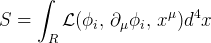
The mismatch between the two senses of symmetry occurs when there is no unitary operator corresponding to the Noether “charge” generating a variational symmetry. Noether's first theorem establishes the existence of a conserved charge for every global variational symmetry of the Lagrangian. The theorem applies to the broad class of theories that derive equations of motion via Hamilton's principle from the action $S=\int_{R}\mathstrut{\cal L} (\phi _{i},\,\partial _{\mu }\phi _{i},\, x^{\mu }) d^{4}x$ , where φ(x) are the dependent variables, x ^μ are the independent variables, and the Lagrangian density is integrated over a compact space-time region R. A solution Φ(x ^μ) is a map from space-time to the space of field variables such that the equations of motion, the Euler-Lagrange equations for , are satisfied. Suppose that there is an r-parameter Lie group G whose elements map $(x,\,\phi) \rightarrow (x^{\prime },\,\phi ^{\prime }) $ such that S is invariant. 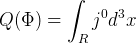Noether's first theorem establishes that there are then r conserved currents, quantities j ^μ(Φ) such that $\partial _{\mu }j^{\mu }(\Phi) =0$ “on-shell” (i.e., for solutions of the equations of motion). The charge associated with the symmetry is the integral of the time component of this conserved current, that is, $Q(\Phi) =\int_{R}j^{0}d^{3}x$ ; it follows from the vanishing divergence of the four vector that Q(Φ) is constant and that $dQ/ dt=0$ , if the current flux vanishes on the boundary of the region R.

If the two senses of symmetry matched, then in the quantized field theory based on this Lagrangian one would find a one-parameter family of unitary operators $\hat{U}(\xi) =e^{i\xi \hat{Q}}$ implementing the symmetry, where $\hat{Q}$ is the operator corresponding to the Noether charge. Fabri and Picasso (Reference Fabri and Picasso1966) showed that if the vacuum state |0〉 is translationally invariant, then the vacuum is either invariant under the internal symmetry, $\hat{Q}\vert 0\rangle =0$ , or there is no state corresponding to $\hat{Q}\vert 0\rangle $ in the Hilbert space.Footnote ⁴ The second case corresponds to SSB. The symmetry is hidden in that there is no unitary operator to map a physical state to its symmetric counterparts; instead, the symmetry is (roughly speaking) a map from one Hilbert space of states to an entirely distinct space. This is usually described as `vacuum degeneracy', although each distinct Hilbert space has a unique vacuum state.

This degeneracy depends on two features of field theory: long-distance or infrared behavior of the fields, and infinite degrees of freedom. Even in the case of classical field theory, the continuity equation for the current j ^μ does not guarantee the existence of a constant of the motion Q _V in the limit $V\rightarrow \infty $ without assumptions regarding the asymptotic behavior of the fields. Parenti, Strocchi, and Velo (Reference Parenti, Strocchi and Velo1977) study the features of SSB in classical, nonlinear field theories; in these theories, solutions to the equations of motion fall into distinct “sectors,” corresponding to global field configurations that cannot be transformed into each other via local perturbations. The variational symmetries of the Lagrangian then fall into the unbroken symmetries, for which Q _V converges in the limit, and broken symmetries, for which Q _V fails to converge. The broken symmetries map between the “physically disjoint worlds” represented by the distinct global field configurations. Similarly, in QFT, the degenerate vacua correspond to distinct global field configurations with minimum energy, with Hilbert spaces built up from a particular vacuum state. Earman's (Reference Earman2003, Reference Earman2004a, Reference Earman2004b) algebraic treatment of SSB emphasizes that these Hilbert spaces are unitarily inequivalent representations of the canonical commutation relations. On the algebraic approach, the fundamental structure of a quantum theory is given by an abstract algebra of the canonical commutation relations, which can be given various different representations in terms of subalgebras of the bounded operators on a Hilbert space. Two such representations, each consisting of a Hilbert space and the set of bounded operators $\hat{O}_{i}$ defined on it, are unitarily equivalent if there is a (one-to-one, linear, norm preserving) map $U\thinspace{:}\thinspace \mathstrut{\cal H} \rightarrow \mathstrut{\cal H} ^{\prime }$ such that $(\forall i) (U^{-1}\hat{O}^{\prime }_{i}U=\hat{O}_{i}) $ . The Stone–von Neumann theorem guarantees that in the finite-dimensional case all irreducible representations of the abstract algebra are unitarily equivalent, but in the infinite-dimensional case there are unitarily inequivalent representations of the algebra.

What the vacuum degeneracy represents physically is perhaps easiest to see in nonrelativistic quantum statistical mechanics, where these ideas were initially developed.Footnote ⁵ Consider, for example, constructing the Hilbert space for an infinite chain of spin-1/2 systems interacting via a specified Hamiltonian. Operators on the Hilbert space of states are linear combinations of the spin operators σ_i for each site, and a state specifies the spin for each system. For any particular global state of the system, such as all σ_z-spin +, there are other states, such as all σ_z-spin −, that cannot be reached by the finite application of spin operators, corresponding to “flipping” the spin of finitely many individual sites. In the case of QFT, the degeneracy corresponds to field configurations that differ globally in a similar sense; particles defined as excitations over distinct vacua cannot be transformed into each other via local operations analogous to flipping the spins at individual sites.

3. Goldstone's Theorem and the Higgs Mechanism

Goldstone's theorem (Goldstone Reference Goldstone1961; Goldstone, Salam, and Weinberg Reference Goldstone, Salam and Weinberg1962) presented a roadblock to using SSB in particle physics. Goldstone showed that breaking a global continuous symmetry implied the existence of massless, spin-zero bosons; this was an unwelcome consequence since there was no place for such Goldstone bosons in the particle physicists’ menagerie. However, several physicists soon exploited the fact that the theorem did not apply to SSB of a gauge symmetry (see Brown and Cao Reference Brown and Cao1991). Anderson was the first to suggest that breaking a gauge symmetry might cure the common problem facing Yang-Mills style gauge theories and SSB applied to particle physics, namely, the prediction of unwanted massless particles. The massless gauge bosons of Yang-Mills theories were not suited to describe short-range interactions like the strong and weak forces. Forcing the issue by adding mass terms directly to the Lagrangian would destroy its gauge invariance and presumably render the theory unrenormalizable. But perhaps the Goldstone bosons could become “tangled up” with the gauge bosons, leaving only a massive gauge boson behind (Anderson Reference Anderson1963, 422); within a year several physicists independently developed different versions of what is now called the Higgs mechanism (Englert and Brout Reference Englert and Brout1964; Guralnik, Hagen, and Kibble Reference Guralnik, Hagen and Kibble1964; Higgs Reference Higgs1964a, Reference Higgs1964b).

Goldstone's theorem shows that the existence of an observable with a nonvanishing vacuum expectation value implies the existence of states whose energy goes to zero as the momentum does; that is, $E(\mathbf{p}) \rightarrow 0$ as $\mathbf{p}\rightarrow 0$ . In relativistic field theory, this implies the existence of massless particles since $E^{2}=m^{2}c^{4}+\mathbf{p}^{2}c^{2}$ . For an intuitive picture, imagine applying the operator $\hat{Q}$ corresponding to the broken symmetry to the vacuum state |0〉. The result would be a distinct vacuum state, but with the same energy since $\hat{Q}$ commutes with the Hamiltonian. Now consider instead the operator $\hat{Q}_{V}$ defined over some finite region V; the states $\hat{Q}_{V}\vert 0\rangle $ should have the same energy as |0〉 except for boundary terms. But since this operator implements a continuous symmetry, the region V can be smoothly deformed so that the boundary terms vanish as $V\rightarrow 0$ , which implies that the energy of the state $\hat{Q}_{V}\vert 0\rangle $ must go to zero for short wavelengths. To make this (slightly) more rigorous, consider an observable $\hat{A}$ whose commutator with $\hat{Q}$ has a nonzero vacuum expectation value, $\mathrm{\lim}_{V\rightarrow \infty }\langle 0\vert [ \hat{Q}_{V},\,\hat{A}] \vert 0\rangle =c\neq 0$ .Footnote ⁶ Rewriting $\hat{Q}_{V}$ as an integral of the charge density, we have $\mathrm{\lim}_{V\rightarrow \infty }\int_{V}d^{3}x\langle 0\vert [ \hat{j}^{0}(\mathbf{x}),\,\hat{A}] \vert 0\rangle =c$ . Assuming that the current is conserved, if the boundary terms vanish then this integral will be time invariant. Manipulation of this expression shows that massive particles would, however, lead to explicit time dependence. For the left-hand side to be nonzero, there must be states |n〉 such that $\langle 0\vert \hat{j}^{0}\vert n\rangle \neq 0$ , with vanishing spatial momenta; these states are the massless Goldstone modes.Footnote ⁷ A full proof of the theorem depends on various standard assumptions in relativistic QFT (see, e.g., Guralnik, Hagen, and Kibble Reference Guralnik, Hagen, Kibble, Cool and Marshak1968), along with the crucial assumption that the commutator $[ \hat{Q}_{V},\,\hat{A}] $ is time invariant in the limit as $V\rightarrow \infty $ .

Higgs (and others who independently discovered the idea) illustrated the gauge symmetry loophole in Goldstone's theorem by constructing simple models that avoid Goldstone bosons.Footnote ⁸ Consider the classical Lagrangian for a complex scalar field φ(x) coupled to electromagnetism,

where $F_{\mu \nu }=\partial _{\mu }A_{\nu }-\partial _{\nu }A_{\mu }$ , the covariant derivative operator is $D_{\mu }=\partial _{\mu }+ieA_{\mu }$ , and V(φ) is the potential for the scalar field, which we will assume to be given by $V(\phi) =\lambda (\phi ^{*}\phi) ^{2}-\mu ^{2}\phi ^{*}\phi $ with $\lambda > 0$ . This Lagrangian has a local U(1) gauge symmetry, $\phi \rightarrow \phi ^{\prime }=e^{-i\xi (x) }\phi $ , under which A _μ transforms as $A_{\mu }(x) \rightarrow A^{\prime }_{\mu }(x) +e^{-1}\partial _{\mu }\xi (x) $ .Footnote ⁹ If $\mu ^{2}< 0$ , V(φ) has a unique minimum at $\phi ^{*}\phi =0$ . However, choosing the “wrong” sign in the potential by setting $\mu ^{2}> 0$ leads to the “Mexican hat” potential, with a ring of minima at $\phi ^{*}\phi =(\mu ^{2}/ 2\lambda) $ . The state of lowest energy is a constant field minimizing the potential. This leads to the natural assumption that in the QFT based on ₁, the quantum field $\hat{\phi }$ will acquire a vacuum expectation value v in the “true” vacuum state. To take the true vacuum state into account, we rewrite the Lagrangian by shifting the field variable, $\phi ^{\prime }=\phi -v$ . Taking advantage of the U(1) gauge invariance allows us to get rid of one degree of freedom of the field entirely by a clever choice of gauge (called unitary gauge), leaving only $\phi ^{\prime }=(1/ \sqrt{2}) (v+\theta (x)) $ .Footnote ¹⁰ These two steps lead to the following Lagrangian:

The second term indicates that the vector field A _μ has become massive, and the third term corresponds to a massive scalar field θ; the ellipsis includes couplings between A _μ and θ, as well as self-interaction terms, but there are no massless scalar fields. The usual way of describing this result is that the massive vector field has “eaten” the would-be Goldstone boson, in the sense that A _μ has acquired the extra degree of freedom required to be massive, namely, a longitudinal polarization state. Finally, there is a trace of the original gauge-invariant Lagrangrian ₁ in the form of relationships that hold between the coupling constants in ₂, and it is these relationships that guarantee renormalizability.

What, exactly, is the “gauge loophole” exploited by this model? The answer depends on the choice of gauge used in analyzing the model (see Guralnik et al. Reference Guralnik, Hagen, Kibble, Cool and Marshak1968; Bernstein Reference Bernstein1974). For some gauge choices, the assumptions of Goldstone's theorem fail to hold; for others, the theorem holds, but the Goldstone bosons “decouple” from the other fields. Treating the QFT based on ₁ in Coulomb gauge, in which $\nabla _{i}A^{i}=0$ (with i ranging over spatial components), there is a nonlocal term analogous to the “instantaneous Coulomb term” that arises in Coulomb gauge QED.Footnote ¹¹ As a result, boundary terms do not vanish in calculating the commutator $\mathrm{\lim}_{V\rightarrow \infty }\int_{V}d^{3}x\langle 0\vert [ \hat{j}^{0}(\mathbf{x}),\,\hat{A}] \vert 0\rangle $ , 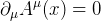which then fails to be a time-invariant constant of the motion—and this was a crucial assumption needed to prove Goldstone's theorem. In Lorentz gauge, $\partial _{\mu }A^{\mu }(x) =0$ , by contrast, the assumptions of Goldstone's theorem hold, and there are Goldstone bosons. However, as with QED, the Lorentz gauge condition cannot be taken as an operator identity, or it would conflict with the canonical commutation relations; instead, one requires that $\langle \phi \vert \partial _{\mu }A^{\mu }(x) \vert \phi \rangle =0$ for all physical states |φ〉 (following the Gupta-Bleuler approach; see, e.g., Schweber [Reference Schweber1962, 242–252]). This subsidiary condition defines the physical states as a subspace of a larger space with an indefinite inner product; the larger space includes “unphysical” or “ghost” states. Imposing the subsidiary condition eliminates the Goldstone bosons, in the sense that they are not part of the physical subspace and have vanishing matrix elements with all physical states.

These striking differences in the mathematical structure of the model with respect to different gauge choices aggravate Earman's worries regarding gauge dependence. The problem arises in other perturbative calculations in QFT. The Green's functions, propagators, and so on are gauge dependent, but the gauge dependence does not matter as long as calculations yield results that are provably gauge invariant (as emphasized by, e.g., Coleman [Reference Coleman1985, 168]). The simple Higgs model described above leads to the same predictions for the masses of the vector and scalar fields in Coulomb and Lorentz gauge (as well as others). But the model includes a number of suspicious gauge-dependent quantities, and next I will turn to the problem of extracting gauge-invariant content.

4. Gauge Dependence of the Higgs Mechanism

The fact that the analysis of Goldstone's theorem depends on the gauge choice may be troubling, but the more essential issue is whether gauge dependence undermines the physical predictions of the Higgs mechanism. The discussion above slid from the identification of the minima of the classical potential V(φ) to the idea that the corresponding QFT should be constructed as a perturbative expansion around this classical minima; however, we should attend to quantum corrections to the classical potential and assess their impact. The effective potential V _eff(φ) was introduced precisely to do this; it agrees with the classical potential V(φ) appearing in equation (1) to lowest order in perturbation theory, but it includes quantum corrections. The true vacua of the field theory are defined by the global minima of V _eff(φ) (setting aside nonperturbative effects). Finding V _eff(φ) exactly requires summing an infinite series of Feynman diagrams in a loop expansion, but one can calculate V _eff(φ) to a given order. The effective potential replaces the classical potential in the procedure above: find the true minima of V _eff(φ), shift the field variables by the vacuum expectation value v, and then calculate quantities using standard perturbation theory techniques. Jackiw (Reference Jackiw1974) first noted a potential problem with this procedure: V _eff(φ) is itself a gauge-dependent quantity, which casts doubt on the physical significance of its minimum.

Physicists explored several different responses to this problem in early studies of the effective potential. One response is to retreat to using only the gauge-invariant classical potential V(φ), the first term of the expansion for V _eff(φ), to define the minima and the vacuum expectation values used to shift the field variables. But this rules out several interesting possibilities. In Coleman and Weinberg's (Reference Coleman and Weinberg1973) important model, SSB occurs due to one-loop quantum corrections; this would be completely missed by the study of V(φ) alone since the classical potential does not exhibit SSB. One can also err in the opposite direction and identify “too many” vacua using the classical rather than the effective potential, a situation called “accidental symmetry” (see Coleman Reference Coleman1985, 142–144). A different response designates one gauge as the “true” gauge. Dolan and Jackiw (Reference Dolan and Jackiw1974) argued that unitary gauge describes the true dynamics without gauge degrees of freedom and, hence, that the effective potential is only physically meaningful in unitary gauge.

Nielsen (Reference Nielsen1975) showed that these earlier responses were unnecessary. He proved that the gauge invariance of various quantities, such as the value of the effective potential at its minima, the mass of the Higgs boson, the mass of the vector boson, and so on, follows from the Ward-Takahashi identities for the Abelian Higgs model. This is analogous to QED, in which the Ward-Takahashi identities express the consequences of gauge invariance for the perturbative evaluation of S-matrix elements (see, e.g., Weinberg Reference Weinberg1995, 442–452). In this case, the identities imply the following partial differential equation for V _eff(φ, ξ), where we have included explicit dependence on the gauge parameter ξ (used to characterize a one-parameter family of gauge choices):

where C(φ, ξ) is calculated by a perturbative expansion. This result implies that the total derivatives of both V _min (the value of the effective potential at the minima) and the Higgs masses with respect to ξ vanish, even though both quantities depend explicitly on ξ and also implicitly on ξ (through the value of φ that minimizes V _eff). As with calculations of S-matrix elements in QED, identities that are ultimately consequences of gauge invariance are imposed on a formalism rife with complicated gauge-dependent expressions in order to ensure that the gauge dependencies do not appear in observable quantities.

5. Breaking a Local Gauge Symmetry?

Shifting from a global to a local gauge symmetry following Higgs and others neatly avoids the consequences of Goldstone's theorem while granting mass to gauge bosons, but how exactly is this connected to SSB as described in Section 2? In one sense the connection is clear: consider an “ungauged” Lagrangian with a global U(1) symmetry, $\mathstrut{\cal L} _{0}=(\partial _{\mu }\phi) ^{\dagger }(\partial ^{\mu }\phi) -V(\phi) $ , alongside the “gauged” Lagrangian, equation (1) above (with the same V(φ)). The symmetry-breaking behavior of the two theories is generally the same; for the Mexican hat potential described above, the global U(1) symmetry of ₀ is broken by the choice of a particular vacuum state—a particular point along the circle of minimum energy—and textbook descriptions use the same language in describing symmetry breaking in ₁. However, the two cases are not similar. Breaking the global symmetry of ₀ leads to vacuum degeneracy, and there are operators that take different expectation values depending on which vacuum state is realized (these are analogues of mean magnetization in a ferromagnet). By way of contrast, all of the states along the minimum circle are fully equivalent in the case of ₁; any particular point along the circle can be mapped to any other via a gauge transformation, and all local operators (such as the $\hat{\phi }$ ) will have the same expectation values regardless of which state is realized.

The contrast between the two cases is reinforced by Elitzur's (Reference Elitzur1975) theorem, which holds in slogan form that “local observables cannot exhibit spontaneous breaking of local gauge symmetry” (Itzykson and Drouffe Reference Itzykson and Drouffe1989, 342). In particular, the theorem shows that although in the case of global symmetry breaking it may be the case that $\langle 0\vert \hat{\phi }\vert 0\rangle \neq 0$ , in the case of local gauge symmetry breaking this quantity (along with the vacuum expectation values of any other gauge-invariant local operator) vanishes. This result threatens to do more than just highlight the difference between gauge and global symmetry breaking. Does it undermine the fundamental assumption of the treatment above, namely, that the Higgs fields acquire nonzero vacuum expectation values? Elitzur proved the theorem in the context of lattice gauge theory, an entirely gauge-invariant formalism that avoids the gauge-dependent quantities appearing in conventional QFT, and the relation of these two different approaches is complicated. But there are two points that mitigate the consequences of Elitzur's theorem. First, the standard account tends not to emphasize the importance of the order of the two separate steps leading up to equation (2): if the gauge is fixed first, then the field operators are no longer gauge invariant and we can set $\langle 0\vert \hat{\phi }\vert 0\rangle =0$ in the perturbative treatment and shift the field variables around this value without running afoul of the theorem; the residual global symmetry may be spontaneously broken, but there is no spontaneous breaking of a local gauge symmetry. The standard accounts typically present the two steps in the opposite order—the field values are shifted, and then one chooses unitary gauge to study the resulting particle spectrum—without assessing whether the two choices are consistent. Second, in this case, Fröhlich, Morchio, and Strocchi (Reference Fröhlich, Morchio and Strocchi1981) give a treatment of the Higgs mechanism in entirely gauge-invariant language, without appealing to the vacuum expectation value of a local observable; the consequences of this treatment agree with the conventional, perturbative account outlined above.

6. Conclusions

Philosophers of physics have begun the difficult task of “lifting the veil” of gauge invariance in order to understand the structure of gauge field theories. This peek behind the veil has revealed, first, that physicists have developed a wide variety of tools for isolating the gauge-invariant content in conventional QFT; the Nielsen identities are one example of how to establish gauge invariance. However, these identities only establish the invariance of the Higgs masses and the minima of the effective potential, leaving open the more general question of the gauge invariance of other quantities appearing in the theory—for example, what is the status of a semiclassical description of the scalar field rolling down the effective potential toward or tunnelling to the minima during a phase transition, an idea invoked in inflationary cosmology? Second, Earman (Reference Earman2003, Reference Earman2004a, Reference Earman2004b) is correct to emphasize that describing the Higgs mechanism as SSB of a local, gauge symmetry is an abuse of terminology. However, it appears to be a relatively benign case of abuse; the consequences of the Higgs mechanism have been rederived within a fully gauge-invariant framework without invoking the suspect notion. Obviously there is much more to be done fully to understand the relationship between these results in lattice gauge theory and the conventional approach, but it will require an extended look behind the veil rather than this brief peek to pin down the Higgs mechanism.