1 Introduction
The flow of a viscous fluid in a cylindrical expansion pipe has been studied for practical reasons in mechanical engineering (Rennels & Hudson Reference Rennels and Hudson2012), food processing (Alberini et al.
Reference Alberini, Simmons, Parker and Koutchma2015) and also in biomedical applications (Vétel et al.
Reference Vétel, Garon, Pelletier and Farinas2008). Although major research of pipe flow had been conducted in a straight pipe, many practical pipe facilities are not straight but have bends, expansions, contractions and so on. Moreover, the flow in a circular pipe with an axisymmetric sudden expansion, at flow rates around the transition to turbulence, is a test case in physiological problems (Zmijanovic et al.
Reference Zmijanovic, Mendez, Moureau and Nicoud2017). This flow consists of a decelerating round jet issuing from the inlet pipe. In addition, the corners of the expansion are responsible for the formation of a recirculation region. The present investigation deals with the case of a laminar flow at the inlet perturbed by a finite amplitude disturbance, which travels and eventually relaminarises downstream of the expansion, if the Reynolds number is below one thousand. The Reynolds number here is based on the inlet diameter
 $d$
as
 $Re=Ud/\unicode[STIX]{x1D708}$
where,
 $U$
is the inlet mean flow velocity and
 $\unicode[STIX]{x1D708}$
is the kinematic viscosity.
The transition to unsteady flow in sudden pipe expansions has been investigated experimentally (Sreenivasan & Strykowski Reference Sreenivasan and Strykowski1983; Pak, Cho & Choi Reference Pak, Cho and Choi1990; Hammad, Ötügen & Arik Reference Hammad, Ötügen and Arik1999; Mullin et al.
Reference Mullin, Seddon, Mantle and Sederman2009) and numerically (Cantwell, Barkley & Blackburn Reference Cantwell, Barkley and Blackburn2010; Sanmiguel-Rojas, Del Pino & Gutiérrez-Montes Reference Sanmiguel-Rojas, Del Pino and Gutiérrez-Montes2010; Sanmiguel-Rojas & Mullin Reference Sanmiguel-Rojas and Mullin2012; Selvam, Peixinho & Willis Reference Selvam, Peixinho and Willis2016). In all these investigations, flow separation after the expansion and reattachment downstream led to the formation of an elongated recirculation region near the wall, with an axial extent that grows linearly with the Reynolds number. Cantwell et al. (Reference Cantwell, Barkley and Blackburn2010) showed numerically that infinitesimal perturbations can grow for
 $Re>26$
and experience significant transient energy growth as
 $Re$
increases. The maximum optimal energy growth values of the first azimuthal mode are of the order of
 $10^{3}$
and
 $10^{6}$
for
 $Re=600$
and 1200, respectively. Experimentally, Mullin et al. (Reference Mullin, Seddon, Mantle and Sederman2009) observed that the flow becomes asymmetric from
 $Re=1139\pm 10$
and the resulting steady flow becomes time dependent at a critical Reynolds number of
 $Re=1453\pm 41$
. These values are much smaller than the predictions of recent numerical stability calculations:
 $Re=3273$
by Sanmiguel-Rojas et al. (Reference Sanmiguel-Rojas, Del Pino and Gutiérrez-Montes2010) or
 $Re=5080\pm 5$
by Cliffe et al. (Reference Cliffe, Hall, Houston, Phipps and Salinger2012). Both works have used an extended computational domain of several hundreds of diameters. This disagreement between numerical simulations and experiments raises the question of the subcritical behaviour of the flow to finite amplitude disturbances. Several numerical studies (Sanmiguel-Rojas & Mullin Reference Sanmiguel-Rojas and Mullin2012; Selvam et al.
Reference Selvam, Peixinho and Willis2016) have found early transition due to finite amplitude perturbations using a tilt type perturbation (along one radial direction) or a vortex type perturbation (along the axial direction with a diameter of a quarter of the inlet pipe diameter), which lead to three-dimensional instabilities and localised turbulent patches. These different perturbations also have different thresholds for transition. Note that in the subcritical regime, the localised turbulent patch relaminarises after the disturbance is removed.
When trying to make connections between theoretical and numerical simulations and experimental observations, a precise temporal and spatial specification of a mathematical perturbation is difficult to replicate in experiments. Ideally, a Dirac
 $\unicode[STIX]{x1D6FF}$
function disturbance is required all around the circumference of the pipe to maintain azimuthal symmetry with zero net mass flux added to the main flow. Some disturbance systems have achieved zero injection and/or subtraction of fluid through slits or holes (Draad, Kuiken & Nieuwstadt Reference Draad, Kuiken and Nieuwstadt1998; Han, Tumin & Wygnanski Reference Han, Tumin and Wygnanski2000). Yet, these disturbance systems created spatially localised turbulent puffs. Practically, the most common disturbance is a single jet through a relatively small hole in the pipe wall (Darbyshire & Mullin Reference Darbyshire and Mullin1995; Hof, Juel & Mullin Reference Hof, Juel and Mullin2003; Peixinho & Mullin Reference Peixinho and Mullin2007; Philip & Cohen Reference Philip and Cohen2010; Tasaka, Schneider & Mullin Reference Tasaka, Schneider and Mullin2010; Mehta & Cohen Reference Mehta and Cohen2016). The main effect of the cross-flow jet is to break the symmetry in a direction perpendicular to the axis. Cross-sectional views of pipe flow downstream of the cross-flow jet have shown the growth of streaks and hairpin vortices (Mellibovsky & Meseguer Reference Mellibovsky and Meseguer2007; Åsén, Kreiss & Rempfer Reference Åsén, Kreiss and Rempfer2010; Philip & Cohen Reference Philip and Cohen2010).
This paper has the aim of quantifying the effect of finite amplitude disturbances, specifically cross-flow, suction and a zero-net-mass-flux synthetic (periodic) jet disturbance on expansion pipe flow. Although synthetic jets have been used to control turbulent flow separation and boundary-layer flow structures leading to hairpin vortices or stretched vortex rings (Jabbal & Zhong Reference Jabbal and Zhong2008; Tang et al. Reference Tang, Salunkhe, Zheng, Du and Wu2014), there is a need for quantitative data in the case of transition to localised turbulence in sudden expansion pipe flow.
A second aim is more general. Using different types of disturbances and quantifying the thresholds for transition to localised turbulence depending on the various parameters, including
 $Re$
, it is believed that the resonator, which is the ability of the flow to self-sustain perturbations, or amplifier dynamics of the sudden expansion pipe flow can be clarified. In § 2, the experimental set-up, the disturbance mechanisms and the visualisation method are presented. In § 3, the results and discussion of the flow visualisation and the thresholds of the different disturbance mechanisms for turbulent patches are presented. Finally, some conclusions are drawn in § 4.
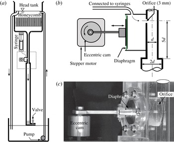
(a) Schematic diagram of the sudden expansion pipe flow apparatus. (b) Schematic of the disturbance mechanism, where the syringe pump connection is used only for injection or suction. (c) Photograph of the synthetic jet mechanism indicating the eccentric cam, the connecting rod, the silicon membrane labelled diaphragm, the cavity and the orifice to the inlet pipe.

2 Experimental set-up
A schematic of the apparatus is shown in figure 1(a). The pipe is made of an assembly of
 $15~\text{cm}$
long transparent push-fitted plastic tubes. The inlet pipe has a diameter of
 $d=10\pm 0.01$
mm and is
 $52.5d$
long with a trumpet shape at the inlet to ensure the flow is fully developed. The following section is
 $97.5d$
long with a diameter of
 $2d$
. The flow is pressure driven. To control the flow rate, the water level into a 50 litre head tank is maintained constant by a spillway and a constant supply of water from a pump. A honeycomb mesh is placed inside the tank to damp unwanted disturbances. The flow rate is then controlled by two fine adjustment valves from Swagelok whose aperture is managed by a graduated screw. The long term temperature stability of the laboratory was controlled to
 $\pm 1\,^{\circ }\text{C}$
at a mean temperature of
 $20\,^{\circ }\text{C}$
. By these means, Reynolds numbers of up to 2000 to within 1 % were achieved.
Figure 1(b) is a schematic diagram of the disturbance mechanism, which consists of a hole of 3 mm diameter (labelled orifice) located at
 $5d$
upstream the expansion. In injection mode, a cross-flow jet was generated using a NE-1600 programmable syringe pump with glass syringes. The disturbance generator is a variant of the system developed by Hof et al. (Reference Hof, Juel and Mullin2003) and, as in their case, the duration and amplitude of the perturbation can be changed independently. They showed that long duration disturbances, corresponding to the localised turbulence length, lead to a well defined threshold for sustained turbulence. Here the duration of the disturbance is also kept long, not less than 90 s. The main parameter describing the amplitude of the disturbance is
 $V_{R}=|V_{j}|/U$
, where
 $V_{j}$
is the jet mean velocity. The same system can be used in suction mode to disturb the flow. Suction has been used in the past as a promising method for maintaining laminar boundary-layer flows (Pfenninger Reference Pfenninger and Lachman1961). Here the suction is through a single hole and the amplitude is also quantified using
 $V_{R}$
.
For the synthetic jet, no syringe pump is used, instead, a motor drives the oscillation of a diaphragm into a cylindrical cavity of 3 cm in diameter and 2 cm in height, connected to the inlet pipe through the
 $3$
mm hole. A photograph of the synthetic jet disturbance system is shown in figure 1(c). Two cams with eccentricities of
 $A=50$
and
 $100~\unicode[STIX]{x03BC}\text{m}$
have been used leading to different oscillation amplitudes. The frequency is set by the rotation speed of the stepper motor, an Orientalmotor PKP series. The motor is computer controlled through an interface card (Arduino UNO). The step resolution, which is
 $0.9^{\circ }$
, allows for oscillations from 0.01 to 10 Hz. The precision of the rotation speed is below
 $1\,\%$
for frequencies under 4 Hz and up to
 $5\,\%$
at 10 Hz.
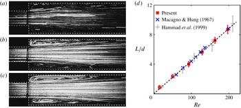
In order to validate the experiment, the axial length,
 $L$
, of the recirculation region as a function of
 $Re$
is shown in figure 2. The photographs in figure 2(a–c) show the particles path lines and the extent of the recirculation region for
 $Re=9$
, 60 and 107 using long exposure type photography. The flow is seeded with
 $50~\unicode[STIX]{x03BC}\text{m}$
spherical particles made of polyamide, with a density of
 $1.018~\text{g}~\text{cm}^{-3}$
. The particles are lit by a 1.5 W green laser sheet. A lens of focal 300 mm is used to zoom at the expansion area. The distortion of the image caused by the pipe’s curvature is reduced by a visualisation box filled with water. Images of the resulting particles field are recorded by a camera which has a sensor of
 $1280\times 800$
pixels,
 $20~\unicode[STIX]{x03BC}\text{m}$
width, leading to a resolution of
 $69~\unicode[STIX]{x03BC}\text{m}~\text{px}^{-1}$
. The images were acquired at 15 Hz for
 $Re=9$
and at 20 Hz for
 $Re=60$
and 107, with an exposure time of 1 ms. The images are then combined to reveal the path lines of particles. In addition, the recirculation region was monitored using two-dimensional particle image velocimetry (PIV). The acquisitions were performed with a high resolution camera (
 $2560\times 2060$
pixels) combined with a zoom (Sigma) of focal 28–300 mm allowing a resolution of
 $50~\unicode[STIX]{x03BC}\text{m}~\text{px}^{-1}$
. The flow was seeded with
 $8{-}11~\unicode[STIX]{x03BC}\text{m}$
hollow-glass spheres with a density of
 $1.1~\text{g}~\text{ml}^{-1}$
and lit by a laser (DualPower 135-15). The vectors fields are computed from Dantec Dynamic Studio software in order to extract
 $L$
. As
 $Re$
increases, the axial recirculation length also increases. In a circular pipe, the recirculation is axisymmetric and pointed in the downstream direction. The PIV experiments show, in figure 2(d), that
 $L$
, is of the form
 $L/d=0.044Re$
, which agrees well with previous experimental (Back & Roschke Reference Back and Roschke1972; Iribarne et al.
Reference Iribarne, Frantisak, Hummel and Smith1972; Latornell & Pollard Reference Latornell and Pollard1986; Hammad et al.
Reference Hammad, Ötügen and Arik1999) and numerical (Cantwell et al.
Reference Cantwell, Barkley and Blackburn2010; Selvam, Peixinho & Willis Reference Selvam, Peixinho and Willis2015) studies for sudden expansion flow. The position of the reattachment point in the downstream part of the recirculation is not trivial to locate accurately because of the wall curvature and light distortion effects. Hence the onset of asymmetric growth could not be detected with the current resolution and is limited to a relatively small range of
 $Re$
.
The flow state was monitored using Kalliroscope as the flow visualant particles or agent. In addition, some experiments were conducted using fluorescein dye. To illuminate the flow, a thin vertical sheet of light was formed using a series of white light sources arranged along the length of the pipe. In some cases a laser sheet was preferred. A camera, mounted on a tripod support, was used to record and monitor the evolution of the disturbances. Typical photographs of the disturbed flow are given in the top image of figure 6(a–c).
Particle path lines of the flow downstream of the expansion for (a)
 $Re=9$
, (b)
 $Re=60$
and (c)
 $Re=107$
. The dashed lines indicate the contour of the expansion. (d) Recirculation length,
 $L/d$
, versus
 $Re$
.
 $\times$
and
 $+$
correspond to previous experimental results (Macagno & Hung Reference Macagno and Hung1967; Hammad et al.
Reference Hammad, Ötügen and Arik1999). The dashed line represents the best-fit proportionality
 $L/d=0.044Re$
.

3 Results and discussion
The results are presented in the form of finite amplitude threshold curves for subcritical transition and space–time diagrams. In injection mode, the threshold for localised turbulence lies in the range
 $0.15\leqslant V_{R}\leqslant 1.3$
for
 $420\leqslant Re\leqslant 1100$
and a hairpin vortex structure has been revealed, whereas in suction mode, the threshold is higher and a significant asymmetry of the flow is observed before the onset of localised turbulence. The final set of results is concerned with synthetic jet disturbances through the same hole. The dependence of the frequency on the amplification of the disturbance along the expansion pipe is quantified.
3.1 Single-jet disturbance
In this experimental set-up at
 $Re\gtrsim 1200$
, disordered flow is initiated naturally by imperfections, roughness, fluid impurities, etc. For
 $400\lesssim Re\lesssim 1200$
, the flow remains laminar and only disturbances of sufficiently large amplitude can initiate localised turbulence. For uniform pipe flow disturbed by cross-flow jets, the dependencies of the flux, the duration, the orientation and the jet diameter were already investigated (Hof et al.
Reference Hof, Juel and Mullin2003; Peixinho & Mullin Reference Peixinho and Mullin2007). Specifically, the critical flux for turbulence is independent of the injection time when the dimensionless disturbed length is larger than 6 pipe diameters. It is also known that smaller jet diameters lead to lower flux thresholds (Peixinho & Mullin Reference Peixinho and Mullin2007; Tasaka et al.
Reference Tasaka, Schneider and Mullin2010).
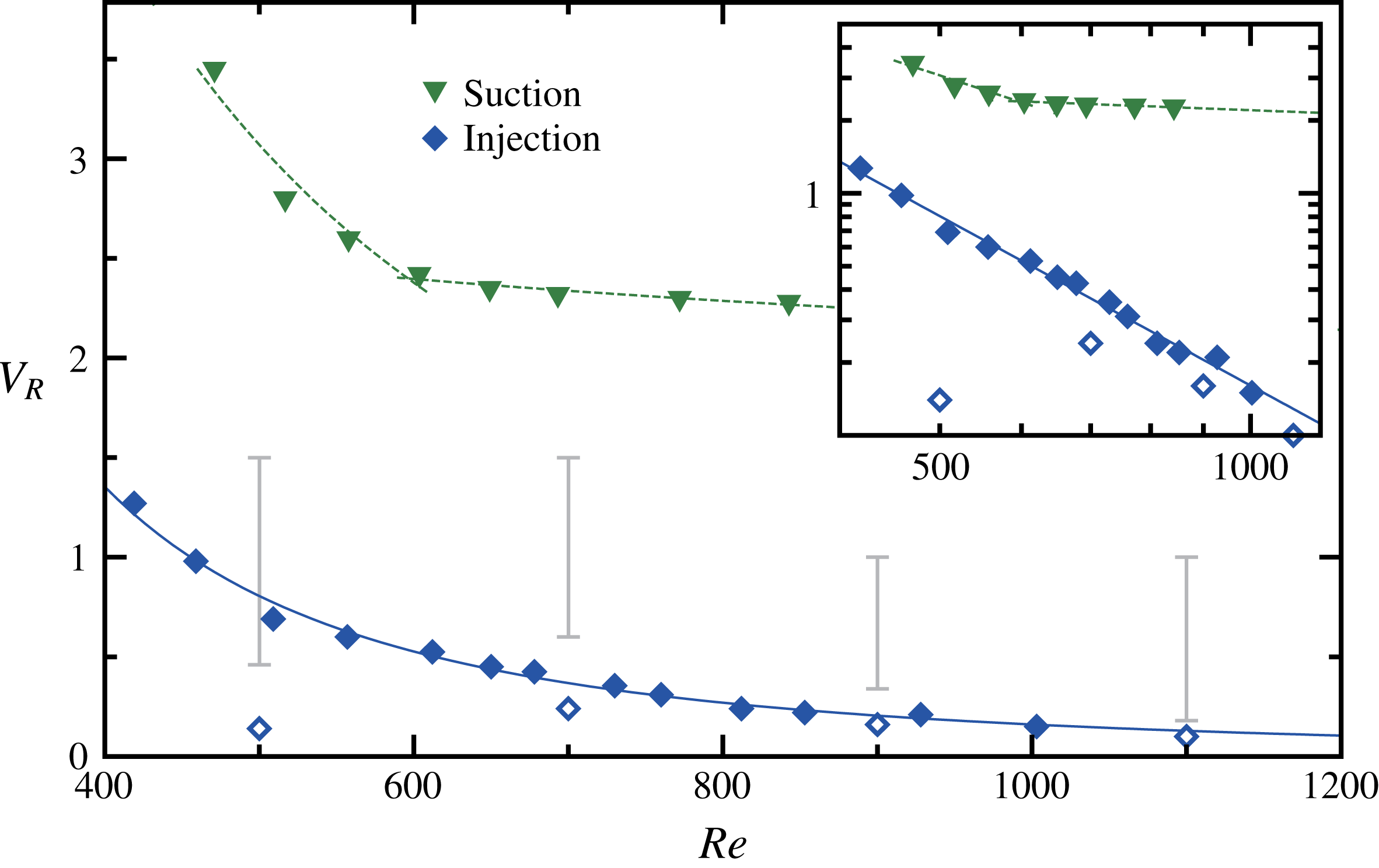
The effect of the cross-flow jet on the sudden expansion pipe flow is shown in figure 3. At small
 $V_{R}$
, the jet modifies the incoming velocity profile, but the flow recovers its laminar state downstream. The flow is considered transient when the laminar state is disturbed for a small fraction of the injection duration (e.g. see figure 4
a) and it is considered above the threshold for localised turbulence when the flow is disturbed for most of the duration of the applied disturbance (e.g. see figure 4
b). In figure 3, the critical velocity ratio,
 $V_{R}$
, decreases with increasing
 $Re$
indicating that the pipe is increasingly sensitive to the jet disturbance. A least-squares fit to the single-jet data gives a good description through a power law:
 $V_{R}\propto Re^{-2.3\pm 0.1}$
. The scaling for subcritical turbulence is fairly abrupt and could be related to the amplification behaviour of the expansion flow. Clearly, the range of
 $Re$
is limited. Furthermore, the scaling cannot hold for smaller
 $Re$
. For
 $Re\lesssim 400$
, disturbances cannot be sustained downstream.
Critical velocity ratio,
 $V_{R}$
, for the onset of localised turbulent patch for single jet and suction as a function of
 $Re$
. The continuous line is a power law fit:
 $Re^{-2.3}$
and the dashed line is a guide to the eye. The error bars indicate the range of parameters where hairpin vortices are observed and open symbols represent visual laminar transient disturbances for the single jet. The inset shows the same results in log–log scale.

Once
 $V_{R}$
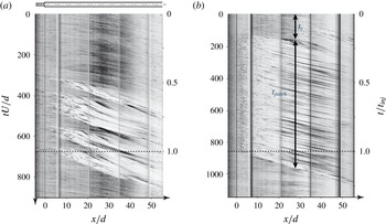
exceeds the threshold, localised turbulence is formed downstream. Typical examples of transient, intermittent and localised turbulent patches are show in the top image of figures 6(a), 6(b) and 6(c), respectively. Figure 4 shows examples of space–time diagrams of the brightness along the centreline axis of the pipe for
 $Re=700$
and 900. The vertical black lines mark the junction between pipe sections. As the single jet is started at
 $t=0$
, the disturbance moves downstream and develops before the localised turbulent patch forms downstream of the expansion at
 $x/d\simeq 3$
. The oblique lines on the diagram represent particles that move downstream and the slope can be related to the mean advection speed of these particles. At
 $t/t_{inj}=1$
,
 $t_{inj}$
being the injection total duration, the injection is stopped and the turbulent localised patch downstream of the expansion decays as it is carried downstream. Below the threshold,
 $V_{R}$
is sufficient to produce disturbed flow that evolves as transient localised turbulence. It is supposed that the injection induces a counter-rotating vortex, typical of a cross-flow jet (Camussi, Guj & Stella Reference Camussi, Guj and Stella2002; Vétel et al.
Reference Vétel, Garon, Pelletier and Farinas2008; Ilak et al.
Reference Ilak, Schlatter, Bagheri and Henningson2012; Karagozian Reference Karagozian2014), which breaks the azimuthal symmetry of the recirculation region downstream of the expansion and induces non-axisymmetric modes as proposed by Cantwell et al. (Reference Cantwell, Barkley and Blackburn2010). Yet, the quantitative identification of such azimuthal modes from the experiments would require three-dimensional PIV and is out of scope of the present study. An example of transient localised turbulence is presented in figure 4(a) for
 $Re=700$
and
 $V_{R}=0.32$
. Supplementary movie 1 (available at https://doi.org/10.1017/jfm.2018.421) shows an example of localised turbulence for
 $Re=700$
and
 $V_{R}=0.35$
.
Space–time diagram of localised turbulence patches (a) below threshold (transient) at
 $Re=700$
and
 $V_{R}=0.32$
, (b) above threshold at
 $Re=900$
and
 $V_{R}=0.54$
.

The dependence of the dynamics of the disturbances on the various
 $V_{R}$
and
 $Re$
was studied through space–time diagrams. These diagrams can be characterised using
 $t_{c}$
, the onset time for the turbulent patch and the patch duration,
 $t_{patch}$
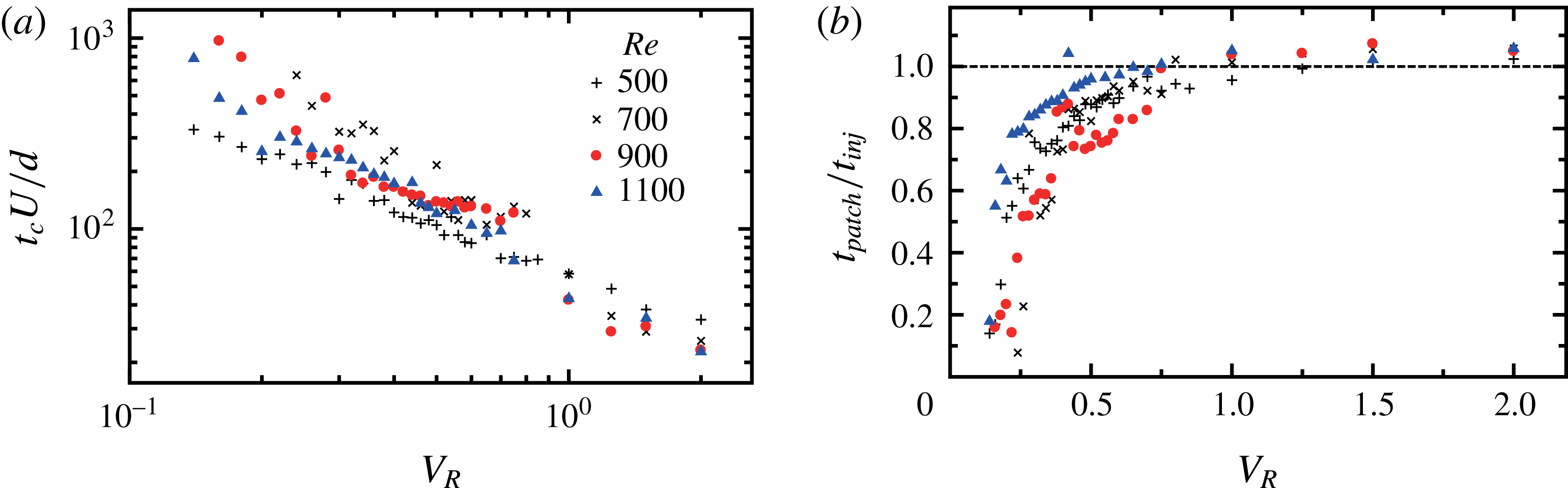
, as sketched by the arrows in figure 4(b). The results of a systematic investigation are presented in figure 5 and show a decrease of
 $t_{c}$
and a rapid increase and saturation of
 $t_{patch}$
as
 $V_{R}$
increases. When scaled by the advection time,
 $U/d$
, the data for different
 $Re$
and different
 $V_{R}$
seem to collapse. Altogether, the data suggest that the subcritical behaviour for single jets depends only on
 $V_{R}$
, the intensity of the jet compared to the mean pipe velocity.
(a) Onset time,
 $t_{c}$
, of the turbulent localised patch as a function of
 $Re$
and (b) variations of duration time of a turbulent patch,
 $t_{patch}$
, with respect to
 $V_{R}$
at different
 $Re$
. The dotted line indicates the end of the injection.

For low
 $V_{R}$
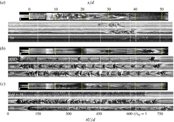
, transient growth and decay of the turbulent patches are observed. In order to describe the spatio-temporal dynamics, figure 6 shows spatio-temporal diagrams for different axial locations along the diameter for
 $Re=700$
. In figure 6(a),
 $V_{R}=0.26$
, the disturbance breaks first at
 $20d$
from the expansion, grows slightly up to
 $x/d=30$
and then decays. In figure 6(b), for
 $V_{R}=0.34$
, an intermittent regime is observed. Finally, in figure 6(c) for
 $V_{R}=0.75$
, the growth remains localised between
 $x/d=10$
and 40.
Flow visualisation photographs and space–time diagrams of transient growth of disturbances at
 $Re=700$
for (a)
 $V_{R}=0.26$
, (b) 0.34 and (c) 0.75. The arrow on the photographs indicates the position of the single-jet disturbance. The dashed-dot lines on the diagrams indicate the end of the jet injection.

3.2 Hairpin vortices
Hairpin vortices have been observed before in uniform pipes (Peixinho & Mullin Reference Peixinho and Mullin2007; Åsén et al.
Reference Åsén, Kreiss and Rempfer2010; Tasaka et al.
Reference Tasaka, Schneider and Mullin2010) or expansion pipe flow (Vétel et al.
Reference Vétel, Garon, Pelletier and Farinas2008). Here, these have been observed specifically for the single-jet disturbance and their domain of existence is indicated by the error bars in figure 3 above the threshold for localised turbulent patches. It is interesting to note that the domain of existence for hairpin vortices appears at
 $0.5\lesssim V_{R}\lesssim 1.5$
. This range of
 $V_{R}$
is in agreement with the range reported in previous studies of jet in cross-flow in large or unbounded domains (Camussi et al.
Reference Camussi, Guj and Stella2002; Ilak et al.
Reference Ilak, Schlatter, Bagheri and Henningson2012; Karagozian Reference Karagozian2014). This suggests that counter-rotating vortex pairs are present in the experiments and may induce instabilities.
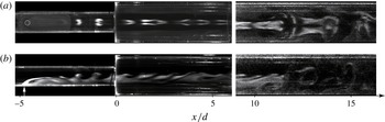
Figure 7 shows these hairpin vortices emerging from a single-jet disturbance at the inlet, propagating through the expansion and breaking down into a turbulent patch. On side view images in figure 7(b), the inclination of the hairpin vortices is enhanced due to the stretching effect when passing through the expansion.
Photographs of a development of hairpin vortex array visualised through fluorescein dye taken for
 $Re=700$
and
 $V_{R}=0.7$
; (a) top view and (b) side view.

3.3 Suction disturbance
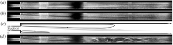
In the case of the suction disturbance, the effect of the aspiration is to distort the inlet velocity profile that induces a strong asymmetry of the flow. A snapshot of the base flow without any disturbance is shown in figure 8(a), and the distorted flows for different
 $V_{R}$
in 8(b) and 8(d), respectively below and above the critical value of
 $V_{R}$
. The vertical white bands correspond to the connections between the pipe sections and the black shadow corresponds to the separation between the two lamps used during acquisition. Figure 8(c) is a sketch illustrating the flow deformation and the position of shear-unstable regions in grey. Specifically, the recirculation area on the opposite side of the aspiration gets several times bigger.
Photographs for the suction disturbance for
 $Re=600$
. (a) Laminar flow:
 $V_{R}=0$
, (b) low amplitude suction at
 $V_{R}=2.2$
, (c) schematic of the streamlines of case (b), where the grey area represents the shear zone, and (d) suction at
 $V_{R}=2.5$
.

Below the critical value of
 $V_{R}$
, transient wavy disturbances appear at the boundary between the main flow and the recirculation area. These are relaminarised without initiating localised turbulence. Supplementary movie 2 corresponds to the case
 $Re=600$
and
 $V_{R}=2.2$
. On the contrary, in figure 8(d),
 $V_{R}$
is above the critical value. The amplification of the instability between the main flow and the recirculation area is observed, the previously mentioned wavy disturbances grow and lead to the formation of a turbulent patch fixed in space. Small disturbances are formed and amplified during the aspiration, sustaining the turbulent patch. In addition, a region of high shear appears at
 $x/d\approx 15$
from the expansion and the analysis of the brightness intensity on the centreline indicates the existence of small amplitude oscillations with a frequency of approximately 0.43 Hz. Such oscillations and frequency have been reported before in numerical simulations (Boujo, Ehrenstein & Gallaire Reference Boujo, Ehrenstein and Gallaire2013; Selvam et al.
Reference Selvam, Peixinho and Willis2015) and their authors have suggested Kelvin–Helmholtz instabilities between the main flow and the recirculation region behind an expansion or a bump.
The finite amplitude thresholds of the suction disturbance for the onset of the localised turbulent patch are also presented in figure 3. Distinct scalings are observed for the jet and the suction. It is also clear that larger
 $V_{R}$
values are required to cause transition. Indeed, the suction preserves the recirculation region and somehow selects axisymmetric modes that require a higher threshold to induce instability. This is consistent with the numerical study of Cantwell et al. (Reference Cantwell, Barkley and Blackburn2010) which showed that the energy growth of azimuthal modes is larger than the axisymmetric ones.
Note that the injection and suction modify the flux in the inlet pipe. Moreover, the scaling for the critical
 $V_{R}$
has a different behaviour as the suction seems to reach a plateau corresponding to a shear consistent with the constant critical velocity required to cause Kelvin–Helmholtz instability. When the suction is stopped, the flow recovers the axisymmetric recirculation pattern after a short transient time.
3.4 Synthetic jet disturbance
In the previous subsections, the cross-flow jet and suction have been tested in a systematic way and indicate clear thresholds for localised turbulence. Now, these disturbances are combined to achieve a periodic zero-net-mass-flux disturbance, since an equal quantity of fluid was pushed then pulled in and out of the pipe through the 3 mm diameter hole. Although periodic excitation is very different from constant-flux disturbances, the periodic injection and suction should lead to essentially the same effect at a very low frequency of oscillation.
Hence, the key parameter is the frequency of the oscillations,
 $f$
, which is made dimensionless through the Strouhal number:
 $St=fd/U$
. The synthetic disturbance was systematically tested for different
 $Re$
and
 $St$
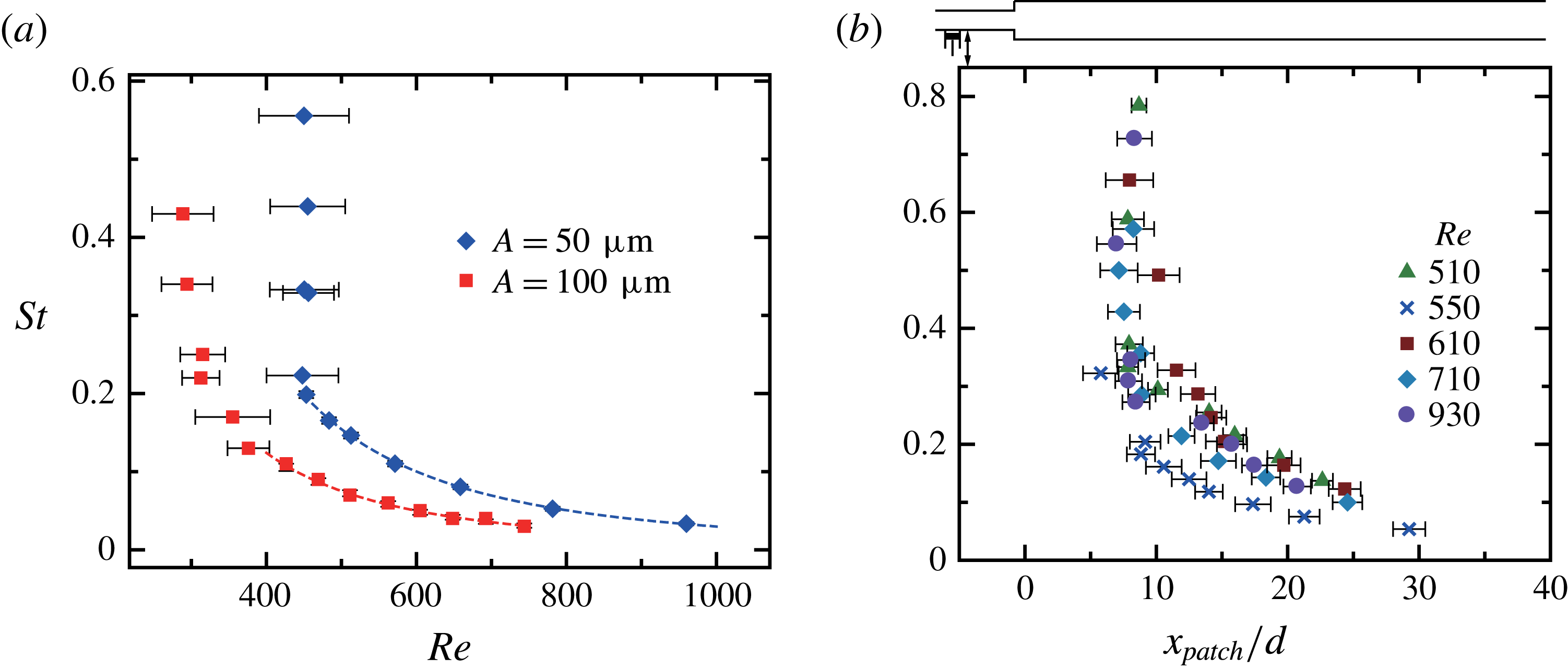
values. Figure 9(a) shows the threshold for localised turbulence as a function of
 $Re$
for two initial oscillation amplitudes:
 $A=50$
and
 $100~\unicode[STIX]{x03BC}\text{m}$
. Note that the values of
 $A$
are relatively small in this study in order to agree with transient growth theory. The general shape of the threshold data is a sharp cutoff at low
 $Re$
and a decreasing curve as
 $Re$
increases, indicating the expansion pipe flow is more sensitive to disturbances of low frequency as
 $Re$
increases. The threshold away from the cutoff can be fitted with a power law:
 $Re^{-2.4\pm 0.2}$
with an exponent similar to the exponent for the single jet. This is because the maximum
 $V_{R}$
can transiently reach values typical of the threshold for a single jet. A systematic shift is observed toward low
 $Re$
and low
 $St$
as the eccentricity of the cam,
 $A$
, is increased. For high
 $St$
, the behaviour of the synthetic jet is basically the periodic formation of stretched vortex rings. As there is a sharp cutoff, the method to estimate the threshold is to keep the oscillation frequency
 $f$
constant and vary
 $Re$
. This leads to horizontal error bars with the left-hand error bar indicating rapid decay of the disturbance and the right-hand a persistence of the disordered motion.
Stability of the synthetic jet disturbance: (a)
 $St$
versus
 $Re$
. The lines are least-square fits:
 $St\propto Re^{-2.2\pm 0.2}$
. (b)
 $St$
versus turbulent patch position,
 $x_{patch}/d$
, for different
 $Re$
and
 $A=50~\unicode[STIX]{x03BC}\text{m}$
. The schematic diagram indicates the position of the disturbance, the expansion and the turbulent patch.

The disturbance involves and forms a localised turbulent patch, which is approximately 25
 $d$
long with an active core and a decaying waves downstream. The location of the active core,
 $x_{patch}$
, remains at a steady axial position from the expansion as long as the disturbance is applied.
 $x_{patch}$
varies sensitively upon
 $St$
and is almost independent of
 $Re$
as shown in figure 9(b). High
 $St$
disturbances caused disturbed flow at
 $x\simeq 7d$
. At
 $St\approx 0.1$
, oscillatory disturbances induced unsteady flow further downstream at
 $x\simeq 25d$
from the expansion.
Transient growth of infinitesimal perturbations has been discussed in various flows (Westin et al.
Reference Westin, Bakchinov, Kozlov and Alfredsson1998; Marais et al.
Reference Marais, Godoy-Diana, Barkley and Wesfreid2011; Boujo et al.
Reference Boujo, Ehrenstein and Gallaire2013; Klotz & Wesfreid Reference Klotz and Wesfreid2017) where the position of the centroid of perturbations is reported to move upstream depending on
 $Re$
and the perturbation frequency. For an expansion pipe, the transient growth analysis from Cantwell et al. (Reference Cantwell, Barkley and Blackburn2010) indicates that stochastic noise-driven flow at
 $Re=600$
and 900 has non-axisymmetric azimuthal modes of disturbances with a centroid of perturbation energy at
 $x/d=18$
and 32, respectively. This is very close to the measured
 $x_{patch}$
reported in figure 9(b). However, the experiment did not show clear periodic optimal flow structures. The simulations of Sanmiguel-Rojas et al. (Reference Sanmiguel-Rojas, Del Pino and Gutiérrez-Montes2010) have predicted the first unstable mode at
 $x\approx 150d$
from the expansion for
 $Re\simeq 3273$
and
 $St\simeq 0.13$
. It suggests that smaller amplitude disturbance could initiate disturbed flow further downstream. In the present experiment, when the disturbance is stopped, the patch is no longer sustained.
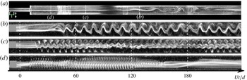
In figure 10, a photograph and space–time diagrams along the pipe diameter at fixed axial positions, where the turbulent patch starts to develop, are presented. Using fluorescein solutions, with a mass concentration of
 $0.001~\text{mg}~\text{l}^{-1}$
, injected at the inlet of the pipe with a flow rate of
 $1~\text{ml}~\text{min}^{-1}$
, the growth of the wavy disturbance can be monitored. The dye travels downstream, passes in front of the disturbance mechanism and then passes through the expansion. Downstream of the expansion, the periodic patterns are captured using the cameras.
Space–time diagrams along the diameter are produced, which show the amplification of the oscillations. Figures 10(b)–10(d) present space–time diagrams for
 $St=0.1$
, 0.17 and 0.42, respectively. Note the
 $x$
-position has to be adjusted and the maximum amplification growth changes with
 $St$
. For
 $St=0.1$
, the amplification occurs at
 $x\simeq 26$
and the wavy disturbance is merely disturbed. For
 $St=0.17$
, the maximum amplification occurs at
 $x/d\simeq 13$
and the space–time pattern contains the main wave and presumably one harmonic. For
 $St=0.42$
, the maximum amplification occurs at
 $x/d\simeq 5$
and seems to contain several harmonics. Yet, no frequency shift is observed upon the main frequency according to fast Fourier transform analysis of the light intensity (not shown). Hence, the synthetic jet disturbance in the range of parameters studied behaves as an amplifier. Further, the space–time diagrams suggest that the instabilities are convective as the flow contains weak or almost no swirl around the axes (Miranda-Barea et al.
Reference Miranda-Barea, Fabrellas-García, Parras and del Pino2016).
The results seem to be consistent with previous experiments from Chun & Sung (Reference Chun and Sung1996), where the turbulent separation flow downstream of a backward-facing step was controlled using a synthetic jet from a thin slit at the corner. The corner location has also been shown to be highly sensitive to disturbances in expansion pipe flow (Sreenivasan & Strykowski Reference Sreenivasan and Strykowski1983; Cantwell et al. Reference Cantwell, Barkley and Blackburn2010). It is anticipated that disturbances introduced further upstream from the expansion may need to be compensated with larger amplitudes to observe transition. Yet, the scalings exponents for the thresholds could still hold and may be used to control the drag or the mixing in the expansion.
Effect of the synthetic jet. (a) A snapshot of the propagating oscillating disturbance from fluorescein visualisation images of the synthetic jet disturbance at
 $Re=600$
and
 $St=0.1$
. See supplementary movie 3. Space–time diagrams at constant
 $x/d$
along the diameter for (b)
 $St=0.1$
at
 $x/d\simeq 26$
, (c)
 $St=0.17$
at
 $x/d\simeq 13$
and (d)
 $St=0.42$
at
 $x/d\simeq 5$
. The location
 $x/d$
corresponds to the trailing edge (upstream) of the disturbed flow.

4 Conclusions
The results of the stability analysis of the flow past a sudden axisymmetric expansion experiencing disturbances have been described. Upstream and downstream pipe sections made of clear transparent material were used to make these observations. Different disturbance mechanisms (i) a single cross-flow jet, (ii) a suction and (iii) a synthetic jet have been tested. With increasing values of the Reynolds number, based on the upstream flow conditions, the flow remains steady and the asymmetry becomes more pronounced for
 $Re\gtrsim Re_{c}$
, where
 $Re_{c}\approx 1200$
is the natural critical Reynolds number of the apparatus. For
 $Re\approx 300$
, the flow becomes sensitive to disturbances, thus the flow visualisation indicates the presence of localised turbulent patches. The single jet is more efficient than the suction in the sense that it requires less flux to initiate turbulence. The threshold amplitude for the simple injection scales with the Reynolds number with a power law exponent of
 $-2.3$
. This exponent is consistent with the possibility of transient growth in the initial steps of the transition process. Moreover, horseshoe structures have been observed for a range of velocity ratios and these are known to appear as a result of cross-flow instability and play a central role in transition to turbulence. The suction disturbance produces a favourable pressure gradient toward the wall and subsequently a strong asymmetry of the recirculation region downstream of the expansion, which nested a shear region between the recirculation and the decelerating jet suggesting a Kelvin–Helmholtz instability.
The stability diagram of the synthetic jet, a zero-net-mass-flux disturbance, has evidenced a threshold at large
 $Re$
with a similar scaling as the cross-flow jet. For low Reynolds number, the synthetic jet has a sharp cutoff for high frequency, which critical Reynolds number is dependent on the oscillation amplitude. At low frequency, the periodic forcing has the advantage of selecting the axial position where the oscillatory flow is amplified and eventually breaks into a localised turbulent patch. In the future, it is planned to study the effect of the expansion ratio, as plane expansions studies (Lanzerstorfer & Kuhlmann Reference Lanzerstorfer and Kuhlmann2012) have shown that the ratio leads to different transition mechanisms depending on the amplification processes: pure centrifugal or elliptical.
Acknowledgements
Our work has benefited from many discussions with T. Mullin. We also thank B. Lechelle and T. Sampo for their technical and engineering support. The authors acknowledge the financial support of the Agence Nationale de la Recherche (ANR), through the project ‘TRANSFLOW’ and the programme ‘Investissement d’Avenir’, LabEx EMC3. Visitation of S.I. at LOMC was supported by JSPS open partnership collaboration research grant. Y.T. was supported by JSPS KAKENHI 15KK0219 and 16H04260.
Supplementary movies
Supplementary movies are available at https://doi.org/10.1017/jfm.2018.421.