

Subnational variation in political preferences across Europe has attracted increasing attention in recent years.Footnote 1 Elections in Europe have repeatedly demonstrated the divergences of political preferences between regions (e.g., Jones et al., Reference Jones, Johnston and Pattie1992; Schraff, Reference Schraff2019). A prominent example is the British vote to leave the European Union (EU), which was informed by strong geographical divides.Footnote 2 The substantial variation in living conditions across the territories of EU members states likely affects a wider range of political preferences (Beramendi, Reference Beramendi2012; Pittau et al., Reference Pittau, Zelli and Gelman2010). Therefore, the regional level is a substantively relevant unit of analysis for our understanding of European politics.
In addition, an investigation of subnational public opinion across Europe holds great promises for innovative research designs in comparative politics. A meso-level perspective provides a good balance between generality (macro-level) and specificity (micro-level) (Georgiadou et al., Reference Georgiadou, Rori and Roumanias2018). Here, regional-level data offers the chance to strengthen causal inference (cf, Rodden, Reference Rodden2010). Usually, country-level data shows limited variability and suffers from many potential confounders. Subnational data allows researchers to hold constant confounding factors from the national level. Further, valid measures of regional preferences enable insightful data description, case selection, and mixed-method designs. Noisy and biased regional opinions can provide a flawed picture of how regions scale on politically relevant dimensions. Consider the example of regional variation in Euroscepticism. Valid estimates of regional preferences are required to adequately rank regions and distinguish between more or less Eurosceptic areas. However, we so far have limited knowledge on regional public opinions as large European comparative social surveys are only representative on the national level. Our paper addresses this gap by evaluating methods for deriving more valid, European-wide regional preferences.
The Eurobarometer (EB) is the European comparative social survey with the broadest temporal and geographical coverage.Footnote 3 However, the EB is not designed to provide representative samples on the subnational level.Footnote 4 In this paper, we use data from regionally representative surveys to evaluate how well we can estimate regional preferences from standard EB data. Our goal is to develop a model that can be applied as a default strategy to estimate various regional political preferences across Europe. Our evaluation study finds that a Bayesian additive regression tree (BART) with synthetic post-stratification provides the best predictions, while requiring less researcher intervention.
1. Predicting regional preferences
In recent years, political scientists have developed various tools to estimate regional public opinion from nationally representative surveys. Below, we shortly introduce the available strategies. Since, we evaluate a number of alternative methods, we have limited space to provide detailed explanations. For more extensive discussions we want to refer readers to literature referenced below.
1.1. Disaggregation
Disaggregation is the simplest strategy to estimate regional preferences from nationally representative survey data. National survey data is disaggregated to the regions respondents reside in. For each region, the average public opinion is calculated, including survey weights if available. This approach is only valid if national surveys have prohibitively large samples or regionally targeted sampling procedures (Hanretty et al., Reference Hanretty, Lauderdale and Vivyan2018).
1.2. Global smoothing in multi-level regression
Current approaches to deal with the noisiness of regional information in the standard EB data apply multi-level regression (Mr) (e.g., Pittau et al., Reference Pittau, Zelli and Gelman2010). The hierarchical structure in the standard EB gives rise to a three-level model, with random effects for countries and regions. Regional estimates should improve due to partial pooling, as sparsely sampled regions more strongly rely on their respective country average. Additionally, good regional predictors should improve predictions by making regions more comparable (Hanretty et al., Reference Hanretty, Lauderdale and Vivyan2018). Regional predictors are also an important extension to the more complicated multi-level approaches introduced below. However, a major short-coming of these methods refers to the selection of regional covariates. Eurostat, for example, offers a rich set of variables on the regional level. Selecting a regional predictor frequently seems arbitrary and brings the risk of overfitting the data.
1.3. Multi-level regression with classical post-stratification
An extension of simple Mr is multi-level regression with post-stratification (MrP). This method gained increasing attention in the past decade and is currently the standard approach for estimating subnational preferences from nationally representative data (Lax and Phillips, Reference Lax and Phillips2009; Warshaw and Rodden, Reference Warshaw and Rodden2012; Buttice and Highton, Reference Buttice and Highton2013; Toshkov, Reference Toshkov2015; Leemann and Wasserfallen, Reference Leemann and Wasserfallen2017; Hanretty et al., Reference Hanretty, Lauderdale and Vivyan2018). MrP comes with the advantages of simple Mr, but additionally allows to correct for systematic differences between the estimation sample and the true population (Lax and Phillips, Reference Lax and Phillips2009; Hanretty et al., Reference Hanretty, Lauderdale and Vivyan2018). Multi-level models are estimated with a set of demographic characteristics (e.g., gender, education, age). Predictions from the multi-level model are then weighted with census data on the true population structure of the demographics.
Data requirements for classical MrP are quite demanding. Researchers need regional census data on all individual-level predictors included in the multi-level model. This comes with a number of challenges. First, census data needs to be congruent with items in the survey data. Education, for example, is measured in the EB as the age when respondents finished full-time education. This is not comparable to regional census data from Eurostat, which reports the highest level of educational attainment. Second, regional census data is only available for a limited set of variables, which are not necessarily good predictors of certain political preferences. Yet, the gains of post-stratification depend on the extent to which individual-level predictors explain regional differences (Leemann and Wasserfallen, Reference Leemann and Wasserfallen2017).
1.4. Multi-level regression with synthetic post-stratification (MrsP)
A recent advancement in the methodological literature is multi-level regression with synthetic post-stratification (MrsP). MrsP addresses some of the weaknesses of classical MrP. More specifically, MrsP allows researchers to use powerful individual-level predictors that are not available from census datasets. The inclusion of such powerful variables can greatly enhance the predictions of regional preferences.
Consider an example where one specifies a model with gender, education, and occupational status as individual-level predictors. Classical MrP requires regional census data on all three predictors for post-stratification: meaning, true joint probabilities. MrsP does not need such detailed data. For MrsP, one collects regional data on the relative gender, education, and occupation shares (regional margins). Joints are created by multiplying margins for each logical combination of the categories of individual-level predictors. These are called synthetic joints because multiplication assumes that individual-level predictors are independent from each other. However, recent research has found that synthetic joints work very well, even if the zero-correlation assumption is violated (Leemann and Wasserfallen, Reference Leemann and Wasserfallen2017).
A major restriction to MrsP is—again—model building. For example, a good individual-level predictor of EU trust is not necessarily a good predictor of redistributive preferences. To build general models, it therefore is important to select variables for synthetic joints that are potentially informative for many political preferences. Otherwise, one risks building idiosyncratic models that do not travel well to other settings.
1.5. Post-stratified BART
A recently proposed alternative to the regression-based methods introduced above is BART (Chipman et al., Reference Chipman, George and McCulloch2012; Montgomery and Olivella, Reference Montgomery and Olivella2018). BART is an ensemble method that estimates many decision trees to subsequently learn the structure of the data. More specifically, BART uses a Bayesian back-fitting algorithm in which each tree tries to accommodate the residuals of the previous tree. The overall fit is derived by regularizing across all trees, which makes each tree a weak learner in the ensemble. There are two major advantages of this tree-based method. First, it is not fitting a global model, but rather estimates highly interactive effects across partitions of the data (a classical tree feature). BART therefore implements deep interactions to predict regional preferences as envisioned by Ghitza and Gelman (Reference Ghitza and Gelman2013). Second, it selects the best predictors and their interactions in an iterative process. This allows researchers to provide a set of predictors and let the algorithm select and interact them in a non-parametric way, just as the data calls for it. As this is done across an ensemble of trees (e.g., 200 trees), we avoid overfitting the data. BART predictions can also be post-stratified with classical or synthetic joints. This provides a further safeguard against bad predictions.
Of course, there are also shortcomings to BART. First, it is a black box method which is more difficult to interpret compared to multi-level regression models. Second, the Bayesian back-fitting algorithm is computationally more costly. Finally, a few hyper-parameters have to be set by the researcher before running the BART model. Researchers have to define the number of trees the BART model should estimate. Here, Chipman et al. (Reference Chipman, George and McCulloch2012) have shown that 200 trees provide reliable predictions. Further, researchers can set parameters for the priors to control the influence of individual trees on the overall fit. We have chosen parameters to ensure a conservative fit by limiting the influence of individual trees.Footnote 5 However, we have varied all hyper-parameters and the resulting predictions remain very similar.
2. Data
We are using the 2015 Standard EB 83.3 to predict regional EU trust and compare the results with the regionally representative data from the 2015 Flash EB. Trust in the EU is the only political preference that is congruently surveyed across both datasets. The 2015 Flash EB provides unique regionally representative public opinions as the sampling procedure is based on randomly drawn telephone numbers from local registers. Moreover, the Flash EB samples 300 respondents per region, which reduces the statistical error substantially compared to Standard EB surveys.Footnote 6 Table A1 in the Appendix provides a more detailed comparison of the sampling procedures. After cleaning and aligning the two datasets, we are able to analyze EU trust across 184 EU regions and 22 member states. Note that we have to omit the very small countries, which do not show subnational variation in the data (e.g., the Baltic states, Malta, Cyprus, and Luxembourg). Depending on the covariates used for post-stratification, the number of regions decreases to 154. The intra-regional correlation for EU trust in the EB 83.3 is 0.04 on the regional and 0.06 on the country level.Footnote 7 This shows that subnational variation is around two thirds of the size of the between-country variation.
We add regional-level predictors from Eurostat to improve the model fit. We retrieve complete regional data on GDP per capita, area size, population density, tertiary education shares, and median household income. We use all regional predictors in the BART model, because the Bayesian back-fitting algorithm does select on the most relevant predictors. However, we have to select manually some variables for the multi-level regressions to avoid overfitting. Therefore, we choose a parsimonious set of predictors for the regression-based methods. Here, we account for the effect of economic conditions on EU trust (Foster and Frieden, Reference Foster and Frieden2017), adding the regional GDP. Moreover, we add a variable measuring whether a region lies in eastern, western, northern, or southern Europe (“grand region”).Footnote 8
For post-stratification, we implement two strategies. First, we apply classical post-stratification using regional demographics from the 2011 census conducted by Eurostat (classical MrP). The 2011 EU census provides a limited set of demographics for all EU regions. The variables that are congruent with the standard EB are gender, age, and marital status. Multi-level regression results are therefore post-stratified by all logical combinations of two gender, six age (ten-year groups from 15 years onward, with the last category being “65 years and older”), and four marital status (single, widow, (re-)married, divorced, or separated) categories.
Second, we implement synthetic post-stratification by adding a promising individual-level predictor. We were looking for a predictor that potentially speaks to many political preferences. This is to ensure a certain generality of the model. We chose the general left–right measure, which is surveyed in the EB regularly. We group respondents into the three categories “left”, “center”, and “right”, and assume that political preferences are informed by the divides across these ideological camps. Margins on left–right self-placement are taken from the regionally representative 2013 Quality of Government survey.Footnote 9 Combining this with regional margins on gender, age, and marital status from the census data allows us to create a table of synthetic joints. Table A3 in the Appendix provides an overview of the data sources and coding schemes for the level-1 predictors.
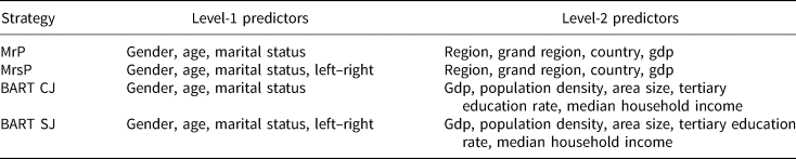
Table 1 presents the different strategies and predictors used in the analysis. Note that the multi-level models are estimated with a reduced set of regional predictors. Contrarily, the BART models include the full set of regional predictors. Here, all regional predictors are country-mean centered to capture the within-country variation. Further, to account for variation between countries, we add the country mean of each regional predictor. This results in a set of 10 level-2 predictors for the BART models.
Overview of predictors and strategies

Regional predictors for the BART models enter the algorithm group-mean centered and as country mean. BART CJ, BART with classical joints; BART SJ, BART with synthetic joints
3. Evaluation results
Figure 1 presents the results of the different estimation strategies with post-stratification (results without post-stratification can be found in Figure A1 of the Appendix). Note that the results are based on the 154 regions for which we have complete data on all variables. For each estimation strategy, we plot the predicted regional mean against the regional representative mean. The 45 degree reference line indicates perfect correspondence. Disaggregation performs worse. The average deviation between predicted and representative values is at 12 percent. Only a third of the predicted values fall into the confidence intervals of the representative values. Table A4 in the Appendix demonstrates that this large degree of noise is present across different datasets and dependent variables. Overall, we find that every method improves upon simple disaggregation.
The performance of prediction strategies.
Notes: r, Pearson's Rho; cov, share of predictions that fall within the 95 percent confidence interval of the representative mean; MAE, Mean Absolute Error; RMSE, Root Mean Squared Error.

A multi-level model with synthetic post-stratification leads to moderate improvements. On average, the predicted mean is off by 9 percentage points from the representative mean. Root Mean Squared Error (RMSE) suggests that estimations are even 12 percentage points off on average. Yet, 44 percent of predicted means now fall within the confidence interval of the representative mean, which is a large improvement. Using only census data for post-stratification—as in classical MrP—improves predictions, though only marginally. Error terms indicate between 8 and 10 percentage points difference and coverage rises to 47 percent. It seems that the left–right orientation does not help the predictive performance of the regression model. Here, classical joints from the census more accurately predict EU trust. Of course, this finding can change for different dependent variables.
A BART model with synthetic post-stratification and regional predictors provides the best predictions. We get an RMSE of around 0.09 and a Mean Absolute Error (MAE) of 0.07. This is a substantial gain in precision. RMSE, for instance, is reduced by 40 percent compared to disaggregation. Coverage increases by 25 points to 58 percent. Now, a clear majority of predictions fall within the confidence interval of the representative means. A BART model with classical joints is somewhat less accurate. Here, coverage is at 54 percent and errors are larger. Even though BART does select on the most relevant predictors, we do not see large gains by adding regional covariates. Most likely, the available regional covariates are not very informative of the outcome. We also see that post-stratification does not make a difference. The raw predictions perform similar to the post-stratified predictions (compare Figure A1 in the Appendix).Footnote 10
A number of insights emerge from our evaluation study. Prediction gains will always depend on the specific modeling strategy. It could well be that there are much better models than the ones we estimated, for example, using individual-level predictors that are more closely related to the outcome variable. These, however, run the risk of being idiosyncratically tuned toward the specific outcome and data under investigation. For instance, one could use trust in national political institutions as a predictor of EU trust, since these two variables have been shown to be substantially related (Muñoz et al., Reference Muñoz, Torcal and Bonet2011). Indeed, we can tune an MrsP model including martial status, age, left–right, and national parliament trust to approach the gains reported under the synthetic BART model. Figure A2 in the Appendix presents the results for this extended MrsP model. The strategy also reaches an MAE of 0.07. This, however, comes at the cost of building a more idiosyncratic model, which could perform worse in new settings.
There is less of a concern regarding overfitting with classical joints, since there is not much of a choice in the selection of individual-level predictors for post-stratification. Currently, only age, gender, and marital status are compatible across the EB and the Eurostat census. Yet, there still is a risk of overfitting coming from the selection of regional predictors. Here, researchers have two options. Either they use MrP, but then they should keep the set of regional predictors parsimonious. Alternatively, researchers can use BART with classical joints to automatize the selection of predictors and capitalize on the other advantages of BART (e.g., deep interactions). In our application, this improved predictions, especially with regard to coverage. Also note that a major advantage of classical joints is that they work for the complete case universe. We therefore recommend using BART with classical joints for applications that require an EU-wide coverage.
For applications that can accept a smaller European-wide sample, synthetic BART is most promising; and, of course, synthetic BART will also be most promising if synthetic joints for all EU regions will become available in the future (using our or other sensible individual-level predictors). In comparison to MrP, BART provides better predictions and reduces the risk of overfitting. Still, a few tuning parameters of the BART model require researcher judgment. However, we have not seen major differences in our predictions when varying them. The Appendix presents the performance of synthetic BART in a new setting. Figure A3 in the Appendix compares disaggregation and synthetic BART for estimating regional social trust in Spain. Here, we use regionally representative data from the QoG survey to validate our results. The predictive performance is equally good.
4. Discussion and outlook
This paper implements a number of strategies to improve regional estimates of public opinion from standard EB surveys. Our evaluation study indicates that BART with synthetic post-stratification performs best, substantially increasing the correspondence between regional estimates and the representative values. MrP and BART with classical joints from the EU census also work well and allow researchers to estimate regional preferences for the complete case universe. We also show that MrsP has great potential, but increases the risk of over-fitting (see Figure A2 in the Appendix). Here, the selection of predictors remains a challenge, asking for careful judgment by researchers.
The paper demonstrates that a lot of choices in the modeling process are dictated by data availability. There is a limited set of variables in the EU census, the regionally representative surveys, and the EBs; and, of course, there are only a few variables that can be measured consistently across the different data sources. A lot of the limitations in our application come from the fact that we estimate regional preferences across the whole EU. This is a highly relevant endeavor for European-wide research. However, it should be noted that there is more potential in estimating regional preferences for single countries, using richer national survey and census data.
Considering our results, one might ask whether the presented gains are “good enough”? Our analysis makes clear that the raw EB data is sub-optimal and that we can improve data quality substantially using estimation procedures. The gains of our analysis are within the range of gains reported in previous evaluation studies (Hanretty et al., Reference Hanretty, Lauderdale and Vivyan2018). Even though the 57 percent coverage reached seems moderate, it substantially exceeds previous results reported for EB data (Toshkov, Reference Toshkov2015). Moreover, Table A5 in the Appendix demonstrates that the reduction in noise affects the substantive interpretations we draw from the data. Table A5 uses regional EU trust as dependent variable in a set of linear regressions and shows that coefficient estimates deviate substantially for the more noisy strategies. However, even our best predictions come with substantial noise. Here, one should consider that our reference values from the Flash EB do have a sampling error.
Even though the substantial noise in EB data is a challenge, we are optimistic that scholars will be able to use the EB's rich regional information. We hope that our analysis lays the ground for the estimation of European-wide regional preferences, enabling more disaggregated comparative research.
Supplementary Material
The supplementary material for this article can be found at https://doi.org/10.1017/psrm.2019.38
Acknowledgments
We thank Thomas König, Lucas Leemann, Matthew Loveless, Santiago Olivella, and Fabio Wasserfallen for helpful comments and advice.