1. Introduction
A strong limitation of biotechnologies comes from the slow growth of cells in large-scale bioreactors (Garcia-Ochoa and Gomez Reference Garcia-Ochoa and Gomez2009). Indeed, diffusion of oxygen is not sufficient to transport these gases deep inside the bioreactor. An additional convective mixing is thus done by introducing bubbles or using rotating blades. However, this creates a strong shear which inhibits the growth of many cells and can even be lethal for fragile cells (Cherry & Papoutsakis Reference Cherry and Papoutsakis1986; Doran Reference Doran1999). For example, the shear around millimetric rising bubbles is of the order of 100 s $^{-1}$ (see Guet & Ooms Reference Guet and Ooms2006). Likewise, a blade rotating at one round per second generates vortices with a vorticity of the order of 10 to 100 s
 $^{-1}$ (see Van't Riet & Smith Reference Van't Riet and Smith1975; Wu, Graham & Noui Mehidi Reference Wu, Graham and Noui Mehidi2006). A bladeless bioreactor with a large mixing rate and a low shear would thus solve a crucial scientific challenge in biotechnologies by increasing the production capacity without damaging the cells.
In the industry, a new generation of bladeless mixers (gyroscopic mixers of the Collomix company, Corob company and Radia company and speedmixers of Flacktek Inc $\ldots$) has been recently introduced for viscous fluids such as paint. These bladeless mixers (called gyroscopic, bi-axial or planetary mixers) create a complex spinning of the container: the pot spins around its axis, the latter being also rotating in a vertical plane. This precessing motion has been largely studied in geophysical fluid dynamics due to the slow precession of the Earth around the north ecliptic pole (Le Bars, Cébron & Le Gal Reference Le Bars, Cébron and Le Gal2015). This motion generates a direct mechanical forcing of the liquid iron in the outer core of the Earth and may be a source of energy for the terrestrial magnetic field (Malkus Reference Malkus1968; Kerswell Reference Kerswell1996; Tilgner Reference Tilgner2007). The flow is very sensitive to precession: it has even been observed for a rotating sphere due to the presence of the rotation of the Earth (Boisson et al. Reference Boisson, Cébron, Moisy and Cortet2012). For a precessing cylinder, the flow is even more energetic due to the resonance of inertial modes at specific aspect ratios (McEwan Reference McEwan1970; Manasseh Reference Manasseh1992, Reference Manasseh1994, Reference Manasseh1996). The viscous saturation can be well predicted analytically by calculating the flow inside the Ekman layers (Gans Reference Gans1970; Meunier et al. Reference Meunier, Eloy, Lagrange and Nadal2008). However, the nonlinear saturation, which is due to the detuning by a mean axisymmetric flow (Meunier et al. Reference Meunier, Eloy, Lagrange and Nadal2008), is more difficult to quantify theoretically because geostrophic flows cannot be forced by an inviscid interaction of a mode with itself (Greenspan Reference Greenspan1969).
In a rotating cylinder, nonlinear interactions can trigger triadic instabilities (Kerswell Reference Kerswell1999): an existing inertial mode can couple the simultaneous growth of two free inertial modes. This mechanism has been observed experimentally in a precessing plane (Mason & Kerswell Reference Mason and Kerswell2002), in a precessing cylinder (Lagrange et al. Reference Lagrange, Eloy, Nadal and Meunier2008) and a precessing annulus (Lin, Noir & Jackson Reference Lin, Noir and Jackson2014). The viscous growth rate can be predicted theoretically, in excellent agreement with the experimental results (Lagrange et al. Reference Lagrange, Meunier, Nadal and Eloy2011). Numerical simulations have confirmed that triadic resonances are responsible for the destabilization of the flow in a precessing cylinder, even for large tilt angles (Albrecht et al. Reference Albrecht, Blackburn, Lopez, Manasseh and Meunier2015, Reference Albrecht, Blackburn, Lopez, Manasseh and Meunier2018; Lopez & Marques Reference Lopez and Marques2018).
Surprisingly, there has been very little attention on the flow inside a rotating cylinder with a fixed axis tilted with respect to the gravity. Yet, Thompson (Reference Thompson1970) showed that the free surface generates a flow similar to the one inside a precessing cylinder. The goal of this paper is to characterize this flow and its mixing properties. First, the laminar flow (§ 3) and its destabilization (§ 4) are measured experimentally and described theoretically. In § 5, the mixing properties (at high Schmidt number) of the flow are measured and compared to those obtained in a classical mixer with blades. The shear is finally measured and compared to that of a mixer with blades in § 6.
2. Materials and methods
2.1. Experimental set-up for a soft mixer
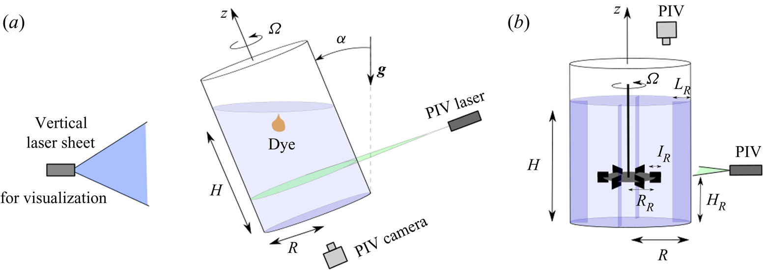
The bladeless mixer under consideration in this paper consists of a circular cylinder rotating around its axis at the angular velocity  $\varOmega$ (see figure 1). The radius
 $R$ of the cylinder ranges from 3 to 9 cm. The cylinder is filled with water up to a height
 $H$, which is defined for a vertical cylinder. The kinematic viscosity
 $\nu$ is deduced from the temperature measurement with an accuracy of 1 %. The axis of the cylinder, defined as the
 $z$-axis, is then slightly tilted by an angle
 $\alpha$ with respect to the gravity
 $\boldsymbol {g}$. The bottom of the cylinder is defined as
 $z=0$ and the vectors
 $\boldsymbol {x}$ and
 $\boldsymbol {y}$ rotate with the cylinder at
 $\varOmega$.
Experimental set-up for the study of (a) a rotating cylinder tilted at an angle  $\alpha$ with respect to the gravity (soft mixer) and (b) a Rushton turbine rotating in a fixed cylinder with four counter-blades.

2.2. Non-dimensional parameters
The fluid problem is governed by four non-dimensional parameters. The aspect ratio  $h=H/R$ is varied from 0.6 to 2.5 in order to capture the three main resonances of the flow. The Reynolds number
 ${\textit {Re}}=\varOmega R^2/\nu$ is varied from
 $10^3$ to
 $10^5$. The tilt angle
 $\alpha$ is varied from 0.5 to 20 degrees in order to get a sufficient forcing for the instability to occur while maintaining a small amplitude of the forced Kelvin mode for the asymptotic theories to remain valid. The Froude number
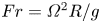 $Fr=\varOmega ^2 R/g$ is smaller than 0.13. Finally, when a passive scalar is injected, an additional parameter arises: the Schmidt number
 $Sc=\nu /\kappa$ (
 $\kappa$ being the molecular diffusivity of the scalar) which is equal to 2500 in our experiments.
2.3. Measurement techniques
Particle visualizations are obtained using a vertical laser sheet and introducing flat mica particles (of average diameter 50  ${{\rm \mu}}$m) covered by titanium dioxide for a better reflexion of light. This technique is well known to highlight qualitatively the coherent structures of the flow (Gauthier, Gondret & Rabaud Reference Gauthier, Gondret and Rabaud1998). It allows measuring the wavelength and the frequency of the three-dimensional (3-D) instabilities.
Particle image velocimetry (PIV) measurements are obtained using a double pulsed yttrium-aluminium-garner laser of 150 mJ per pulse at 532 nm. The camera is located below the cylinder (which has a transparent polymethyl methacrylate bottom) rather than above the cylinder in order to prevent distortions of the images by the free surface. The images are rotated numerically in order to remove the mean solid body rotation of the flow. The perturbations of the flow due to the tilt angle can thus be magnified by increasing the time interval between the two frames to about  $0.1/\varOmega$ (which leads to a rotation of the cylinder of
 ${\sim }5^{\circ }$ between the two frames). The 4 megapixel image pairs acquired at about 1 to 2 Hz are then treated by a homemade cross-correlation algorithm optimized for large velocity gradients (Meunier & Leweke Reference Meunier and Leweke2003) with window sizes equal to
 $32^2$ pixels. The velocity and axial vorticity fields are obtained in two different sections of the cylinder (
 $z=H/2$ and
 $z=H/4$). The uncertainty on the vorticity is found to be approximately 1 % in the nearly laminar regime.
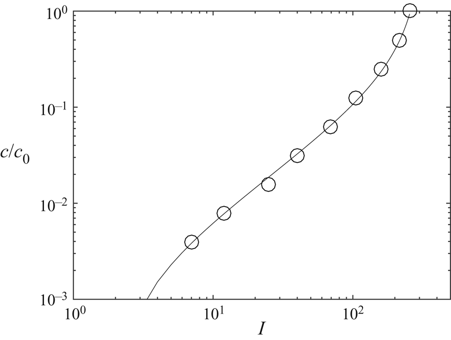
A third measurement technique was used in order to quantify the mixing efficiency of the flow. A blob of fluorescent dye (Fluorescein) is introduced just below the free surface and illuminated by a continuous laser sheet from a 400 mW laser at 488 nm. The emitted intensity  $I$ is calibrated after each experiment by introducing inside the cylinder small tubes containing calibrated concentrations of Fluorescein. The calibration curve plotted in figure 2 indicates that the concentration
 $c$ is well fitted by a law of the form
 \begin{equation} \frac{c}{c_0} = \alpha \frac{I-I_0}{I-I_{{sat}}} \end{equation}
over more than 2 decades in concentration and with an accuracy of at least 10 %. The term  $I_0$ corresponds to the intensity of the background of the images and the term
 $I_{{sat}}$ takes into account the saturation of the dye emission and the nonlinearity of the camera sensor. This calibration allows measuring the concentration in a vertical and meridional section during the mixing process with about 1 million pixels in each image at a rate of 25 frames per second.
Calibration curve between the intensity of the pixels on the images and the concentration  $c$ in Fluorescein.

2.4. Experimental set-up for a Rushton turbine
The mixing properties of the soft mixer are compared to the mixing properties of a classical Rushton turbine in a cylinder of radius  $R=9$ cm filled at a height
 $H=2R$ (see figure 1b). The turbine consists of six vertical square blades of size
 $l_R=H/9$ fixed on a horizontal rotating disk of radius
 $R_R=H/3$ at a height
 $H_R=H/3$. Four vertical counter-blades of side
 $L_R=H/6$ are fixed to the cylinder in order to block the solid body rotation of the fluid. As in the case of the soft mixer, the Reynolds number is based on the cylinder's radius
 ${\textit {Re}}=\varOmega R^2/\nu$. It is varied between 1000 and 20 000. Dye visualizations are done in a vertical section and PIV measurements in a horizontal section 1 mm above the rotating disk.
3. Resonant forcing of inertial modes
For small Froude numbers, the free surface remains horizontal. In the frame of reference of the cylinder, it is thus located at
 \begin{equation} z=H+\eta(r,\theta) \quad \mathrm{with}\ \eta(r,\theta)=-\alpha r \cos(\theta + \varOmega t). \end{equation}
This means that the free surface has a rotating sloshing at  $-\varOmega$ around the (tilted) axis of the cylinder. It is very similar to the experiment done by McEwan (Reference McEwan1970) where the forcing was done by a rigid plate rather than the free surface. This motion with respect to the fluid excites inertial waves in the bulk of the rotating fluid. These waves interfere constructively to form global Kelvin modes (Kelvin Reference Kelvin1880). Following the calculations of Thompson (Reference Thompson1970) for small tilt angles and small Froude number, the velocity must be a solution of the linearized Navier–Stokes equations in the frame rotating with the cylinder
 \begin{equation} \frac{\partial {\boldsymbol{\mathsf{u}}}}{\partial t} + 2 \varOmega \hat{\textbf{z}} \times \boldsymbol{u} = -\frac{\boldsymbol{\nabla} p}{\rho_0} + \nu \nabla^2 \boldsymbol{u}, \end{equation}
together with the incompressibility
 \begin{equation} \boldsymbol{\nabla} \boldsymbol{\cdot} \boldsymbol{u} =0. \end{equation}
Here, the reduced pressure is defined as  $p=P-\rho gz+\rho r^2\varOmega ^2/2$ where
 $P$ is the total pressure. This allows for removing the buoyancy force and the centrifugal force from the Navier–Stokes equations. In the limit of large Reynolds numbers, the velocity is searched as a sum of Kelvin modes (which are solutions of the linearized Euler equations). Using cylindrical coordinates, this can be written
 \begin{equation} \boldsymbol{u} = \left(\begin{array}{@{}c@{}} u^r \\ u^\theta \\ u^z \end{array}\right) = \sum_{i=1}^{\infty} \frac{a_i}{k_i R} \textrm{Re} \left[\left(\begin{array}{@{}c@{}} u^r_i(r) \cos(k_i z) \\ u^\theta_i(r) \cos(k_i z) \\ u^z_i(r) \sin(k_i z) \end{array}\right) \exp({\,j(\theta + \varOmega t)}) \right] ,\end{equation}
with
 \begin{equation} \boldsymbol{u}_i = \left( \begin{array}{@{}c@{}} u^r_i(r) \\ u^\theta_i(r) \\ u^z_i(r) \end{array} \right) = \left( \begin{array}{@{}c@{}} k_i R J'_1(\sqrt{3}k_i r)/\sqrt{3} + 2 \textrm{J}_1(\sqrt{3}k_i r) R/(3 r) \\ 2 j k_i R J'_1(\sqrt{3}k_i r)/\sqrt{3} + j \textrm{J}_1(\sqrt{3}k_i r) R/(3 r) \\ - j k_i R \textrm{J}_1(\sqrt{3}k_i r) \end{array} \right), \end{equation}
where  $\textrm {J}_1$ is the Bessel function of the first kind,
 $\textrm {Re}$ is the real part and
 $j=\sqrt {-1}$. The pressure is given by
 \begin{equation} p= \sum_{i=1}^{\infty} \frac{a_i \rho_0 \varOmega}{k_i} \textrm{Re} \left[ p_i(r) \cos(k_i z) \exp({\,j(\theta+\varOmega t)}) \right]\quad \mathrm{with} \ p_i(r) = \textrm{J}_1(\sqrt{3}k_i r). \end{equation}
The boundary conditions of vanishing radial velocity  $u_i^r(r)$ at
 $r=R$ sets the value of the wavenumber of each Kelvin mode
 \begin{equation} k_1 R = 1.579,\quad k_2 R = 3.286,\quad k_3 R = 5.062\ldots. \end{equation}
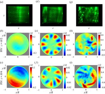
Figure 3(b,c) shows the cross-cut velocity fields when the height of fluid  $H$ is equal to
 $2R$. The cross-cut velocity at a quarter of height (
 $z=H/4$) exhibits a strong jet created by two counter-rotating vortices facing each other along the diameter. This structure corresponds to the first Kelvin mode since the axial vorticity, given by
 \begin{equation} \zeta = 2 k_i a_i \cos(k_i z) \sin(\theta + \varOmega t) \textrm{J}_1(\sqrt{3} k_i r) \end{equation}
has an azimuthal wavenumber  $m=1$ and contains only one lobe between
 $r=0$ and
 $r=R$ for the first mode (since
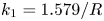 $k_1=1.579/R$). By contrast, at mid-height (
 $z=H/2$), the velocity field is very small because it corresponds to a node of the axial vorticity at this axial position and for this specific aspect ratio
 $H/R=2$.
Visualizations (a,d,g) and PIV measurements (b,c,e,f,h,i) of the 2-D velocity and axial vorticity  $\zeta$ in the cross-section. The cylinder of radius
 $R=4.6$ cm is filled with water up to a height
 $H=9.2\ \textrm {cm}= 2R$ to excite the first resonance of the first mode. The angular velocity
 $\varOmega$ of the cylinder increases from 0.47 rad s
 $^{-1}$ (a–c) to 2 rad s
 $^{-1}$ (d–f) and then 4.7 rad s
 $^{-1}$ (g–i). The cylinder's axis is tilted at an angle
 $\alpha =1^\circ$ with respect to the gravity. In (e–f) measurements have been obtained during the growth of the instability and the mean flow has been subtracted. Movies corresponding to figures 3(e) and 3(f) are available as supplementary files at https://doi.org/10.1017/jfm.2020.634. (a) Re = 1000: stable flow, (d) Re = 4300: instability, (g) Re = 10 000: turbulence.

The amplitude  $a_i$ of the
 $i$th mode is governed by the boundary condition at the free surface. The axial velocity must be equal at
 $z=H+\eta (r,\theta )$ to
 \begin{equation} u^z = \alpha \varOmega r \sin(\theta + \varOmega t) .\end{equation}
For small tilt angles, this boundary condition can be applied at  $z=H$ since the difference between the velocity at
 $z=H$ and at
 $z=H+\eta$ scales as
 $\alpha ^2$. The boundary condition (3.9) can be satisfied at
 $z=H$ in the inviscid limit if the coefficients
 $a_i \sin (k_i H) / k_i$ correspond to the coefficients of the Dini series of the function
 $\alpha \varOmega r$. The quantitative value of these coefficients can be found by introducing (3.4) and (3.5) into (3.9), multiplying by
 $r \,\textrm {J}_1(\sqrt {3}k_i r)$ and by integrating over
 $r$ (see Thompson Reference Thompson1970). This leads to
 \begin{equation} a_i = \frac{\displaystyle\int_0^R r^2 \,\textrm{J}_1(\sqrt{3}k_i r)\,\textrm{d} r}{\displaystyle\int_0^R r \,\textrm{J}_1^2(\sqrt{3}k_i r)\,\textrm{d} r R \sin(k_i H)} \alpha \varOmega R .\end{equation}
Numerically it gives a simple expression for mode 1
 \begin{equation} a_1= \frac{1.330 \alpha \varOmega R}{\sin(k_1 H)} .\end{equation}
It is clear from this expression that the amplitude of the  $i$th mode diverges when
 $\sin (k_i H)$ vanishes, i.e. when the height of fluid
 $H$ is equal to a multiple of a half-wavelength
 ${\rm \pi} /k_i$. This resonant situation corresponds to the case when the free surface is located at a node of axial velocity of the
 $i$th mode. The amplitude of the forced mode must thus become very large in order to create a finite axial velocity of the free surface as required by the boundary condition (3.9). The resonances of the
 $i$th mode are thus obtained for
 $k_i H = n {\rm \pi}$ with
 $n$ an integer. For example, the resonances of the first mode are found for
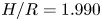 $H/R=1.990$,
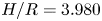 $H/R=3.980$,
 $H/R=5.970\ldots$ However, in this paper, we will restrict our attention to the first resonance of this mode. Other Kelvin modes (corresponding to
 $k_2$,
 $k_3\ldots$) can also be observed. In this paper, we will also study the first resonance (i.e.
 $n=1$) of the second mode (obtained for
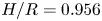 $H/R=0.956$) and the first resonance of the third mode (obtained for
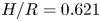 $H/R=0.621$).
Obviously, the amplitude  $a_i$ of the global inertial mode at the resonance is saturated by viscous effects. Ekman pumping creates a normal flow at order
 ${\textit {Re}}^{-1/2}$ which compensates the vanishing normal velocity of the mode at the resonance. This effect can be calculated analytically (see appendix A) using a solvability condition which takes into account both Ekman and volumic damping as in Gans (Reference Gans1970). This leads to the amplitude around the resonance
 \begin{equation} a_i=\frac{F/T}{-\sin(k_i H) + (B+C)/(T\sqrt{{\textit{Re}}}) + V/(T {\textit{Re}})} \alpha \varOmega R, \end{equation}
where the coefficients  $F$,
 $T$,
 $B$,
 $C$ and
 $V$ are given analytically in the appendix A. Neglecting the volumic attenuation (scaling as
 ${\textit {Re}}^{-1}$) in front of the Ekman damping (scaling as
 ${\textit {Re}}^{-1/2}$), the amplitude at the resonance can be written
 \begin{equation} a_i= \frac{F}{B+C} \alpha \varOmega R \, Re^{1/2}, \end{equation}
where the coefficient  $|F|/|B+C|$ is equal to 0.309, 0.0815 and 0.0318 for the three first modes. Because of the resonance of the inertial waves, this amplitude can be large even for small tilt angles. For example, figure 3(a–c) shows that even 1 degree of tilt is sufficient to create a vorticity
 $\zeta$ equal to 20 % of the angular velocity
 $\varOmega$ at
 $r \approx 0.65 R$. This is in excellent agreeement with the theoretical prediction (3.8) which predicts that the maximum vorticity is equal to
 $0.221 \varOmega$ at
 $r=0.673 R$. This strong flow can possibly destabilize the flow, as will be shown in the next section.
4. Parametric instability by triadic resonance
4.1. Experimental observations
When the Reynolds number increases from 1000 to 4300, the flow becomes unstable and ceases to be stationary. Qualitative flake visualizations of figure 3(a,d) indicate that the axis of rotation visible at  $Re=1000$ disappears. It is replaced by columns located at the periphery of the cylinder. If the Reynolds number is increased up to
 ${\textit {Re}}=10\,000$, the instability becomes more and more energetic and generates small-scale structures, as shown in figure 3(g).
This instability is very similar to the instabilities observed in a precessing flow where it is due to a triadic resonance between the forced Kelvin mode and two other free modes. Such an instability has been found inside a precessing plane (Mason & Kerswell Reference Mason and Kerswell2002), inside a precessing cylinder (Lagrange et al. Reference Lagrange, Eloy, Nadal and Meunier2008, Reference Lagrange, Meunier, Nadal and Eloy2011; Albrecht et al. Reference Albrecht, Blackburn, Lopez, Manasseh and Meunier2015) and inside a precessing annulus (Lin et al. Reference Lin, Noir and Jackson2014). This mechanism, also called parametric instability, is classical for surface waves, where a harmonic wave can excite two sets of waves with different wavelengths (Craik & Leibovich Reference Craik and Leibovich1976; Miles & Henderson Reference Miles and Henderson1990; Francois et al. Reference Francois, Xia, Punzmann and Shats2013). This process is also found for internal waves in stratified flows (Staquet & Sommeria Reference Staquet and Sommeria2002; Dauxois et al. Reference Dauxois, Joubaud, Odier and Venaille2018; Thomas & Yamada Reference Thomas and Yamada2019) and for inertial waves in rotating flows (Yarom & Sharon Reference Yarom and Sharon2014), where it generates wave turbulence. For a precessing cylinder, Lagrange et al. (Reference Lagrange, Meunier, Nadal and Eloy2011) predicted theoretically that the most unstable free modes have azimuthal wavenumbers  $m'=5$ and
 $m''=6$ for a large range of aspect ratios. It is also the case in this experiment for the first resonance of the first mode (i.e. at
 $H/R=2$), as shown in figure 3(e,f). At mid-height, the instability exhibits a ring of six positive and six negative vortices (see supplementary movie 1). By contrast, at a quarter of height, the instability contains five positive and five negative vortices (see supplementary movie 2).
It indicates that the mode 5 has a node of vorticity at mid-height (i.e.  $\zeta \sim \cos (k'z)$ with
 $k'={\rm \pi} /H$) whereas the mode 6 has two nodes of vorticity at one-quarter and three-quarter height (i.e.
 $\zeta \sim \cos (k''z)$ with
 $k''=2{\rm \pi} /H$). This is consistent with the theory which requires the triadic resonance condition
 \begin{equation} k''-k' = k_1, \end{equation}
where  $k_1={\rm \pi} /H$ is the axial wavenumber of the forced mode. The same resonance condition
 \begin{equation} m'' - m' = m_1 \end{equation}
is obviously fulfilled for the azimuthal wavenumbers  $m'=5$ and
 $m''=6$ since the forced mode has an azimuthal wavenumber
 $m_1=1$. The last necessary condition concerns the frequencies of the modes
 \begin{equation} \omega'' - \omega' = \varOmega. \end{equation}
This relation is respected only for modes  $m'=5$ and
 $m''=6$ (since the frequencies are determined by the dispersion relations
 $\omega '(k',m')$ and
 $\omega ''(k'',m'')$ of the Kelvin modes). To conclude, these experimental observations clearly prove that this instability is due to a triadic resonance between two free Kelvin modes with wavenumbers
 $(k',m')$,
 $(k'',m'')$ and the forced Kelvin mode with wavenumbers
 $(k_i,1)$.
4.2. Linear stability analysis
A linear stability analysis is performed assuming that the flow is the sum of a forced Kelvin mode  $\boldsymbol {u}_i$ of amplitude
 $a_i$ and two free Kelvin modes
 $u'$ and
 $u''$. The velocity field is searched as
 \begin{align} \boldsymbol{u} &= \frac{a_i}{4 k_i R} \boldsymbol{u}_i \exp({\,j(\pm k_i z + \theta + \varOmega t)}) + a' \boldsymbol{u}' \exp({\,j(\pm k' z + m' \theta + \omega' t)}) \nonumber\\ &\quad + a'' \boldsymbol{u}'' \exp({\,j(\pm k'' z + m'' \theta + \omega'' t)}) +\mathrm{c.c.}, \end{align}
where c.c. corresponds to the complex conjugate and where  $\pm k$ indicates that the term with a positive wavenumber must be added to the same term with a negative wavenumber. The first term corresponds to the resonant Kelvin mode defined in (3.4). The wavenumbers
 $k'$ and
 $k''$ of the free modes must be multiples of
 ${\rm \pi} /H$ in order for the free modes to respect the boundary conditions
 $u^z=0$ at the top and bottom. The radial structure of the free modes
 $\boldsymbol {u}'$ and
 $\boldsymbol {u}''$ are given in the appendix A.
If the three resonance conditions are satisfied, the nonlinear interaction of the forced mode  $\boldsymbol {u}_i$ and the free mode
 $\boldsymbol {u}'$ can force the temporal derivative of the second free mode
 $\boldsymbol {u}''$. Assuming that the amplitude
 $a'$ is slowly varying in time, the amplitude equation for the first mode can be calculated (see appendix A) leading to
 \begin{equation} \frac{\partial a'}{\partial t} = N' a'' \frac{\overline{a_i}}{4 k_i R^2 \varOmega} - D' a', \end{equation}
where  $\bar {\cdot }$ is the complex conjugate. The same mechanism occurs for the temporal derivative of the first free mode
 $\boldsymbol {u}'$. A similar amplitude equation can be found for mode
 $\boldsymbol {u}''$
 \begin{equation} \frac{\partial a''}{\partial t} = N'' a' \frac{a_i}{4 k_i R^2 \varOmega} - D'' a''. \end{equation}
All coefficients can be calculated analytically. They are given in the appendix A. The coefficients  $N'$ and
 $N''$ come from the nonlinear coupling of the forced mode with a free Kelvin mode. The second terms on the right hand side correspond to detuning and dissipation terms. Their coefficients are given by
 \begin{equation} \left.\begin{gathered} D' = \frac{S'}{\sqrt{{\textit{Re}}}} + \frac{V'}{{\textit{Re}}} + j Q' {\rm \Delta} k', \\ D'' = \frac{S''}{\sqrt{{\textit{Re}}}} + \frac{V''}{{\textit{Re}}} + j Q'' {\rm \Delta} k'', \end{gathered}\right\} \end{equation}
where the first terms correspond to surface Ekman pumping, the second terms correspond to volumic dissipation and the third terms correspond to detuning. All the coefficients are given analytically in the appendix A. For example, the nonlinear coefficients are equal to  $N'=-1.216$ and
 $N''=-1.94$ for modes
 $m'=5$ and
 $m''=6$ at
 $H/R=2$.
In the absence of detuning/dissipation terms,  $a'$ and
 $a''$ grow exponentially as
 $\textrm {e}^{\sigma t}$, which leads to an exact prediction for the inviscid growth rate
 \begin{equation} \sigma = \sqrt{N' N''} \frac{|a_i| }{4 k_1 R^2}. \end{equation}
When dissipation/detuning effects are taken into account the growth rate  $\sigma$ becomes complex and solution of a second-order equation (see appendix A). The real part of the growth rate vanishes when the amplitude of the forced Kelvin mode is equal to
 \begin{equation} |a_i| = 4 k_i R \left\{ \frac{\textrm{Re}(D')\textrm{Re}(D'')}{N'N''} \left[ 1+ \frac{{\rm Im}(D'-D'')^2}{\textrm{Re}(D'+D'')^2} \right] \right\}^{1/2} \varOmega R, \end{equation}
where  ${\rm Im}$ is the imaginary part. Equating this formula with the amplitude
 $a_i$ of the Kelvin mode forced by the tilted free surface (3.12) gives the value of the critical angle
 $\alpha$ at which the flow becomes unstable
 \begin{align} \alpha = \frac{4 k_i R}{|F|} \left\{ \frac{\textrm{Re}(D')\textrm{Re}(D'')}{N'N''} \left[ 1+ \frac{{\rm Im}(D'-D'')^2}{\textrm{Re}(D'+D'')^2} \right] \right\}^{1/2} \left| -T \sin(k_i H) + \frac{B+C}{\sqrt{{\textit{Re}}}} + \frac{V}{{\textit{Re}}} \right| . \end{align}
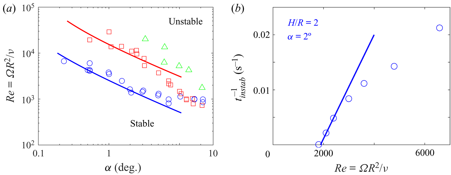
This theoretical prediction is plotted as solid lines in figure 4(a) as a function of the tilt angle. It is in excellent agreement with the experimental measurement of the instability threshold (plotted as symbols) for angles smaller than 10 degrees despite the absence of fitting parameter in the model. It should be mentioned that this critical Reynolds number is determined experimentally for each angle as the value for which the onset time of the instability  $t_{onset}$ becomes infinite (determined from a linear fit of
 $t_{onset}^{-1}$ as a function of Re as in figure 4b).
(a) Stability diagrams for fixed aspect ratios corresponding to the resonance of mode 1 (blue  $\circ$,
 $H/R=2$), of mode 2 (red
 $\square$,
 $H/R=1$) and of mode 3 (green
 $\triangle$,
 $H/R=0.6$). Symbols correspond to experimental measurements of the threshold. Solid lines correspond to theoretical predictions with no fitting parameter as given by (4.10). (b) Example of the onset time of the instability
 $t_{instab}$ as a function of the Reynolds number measured for mode 1.

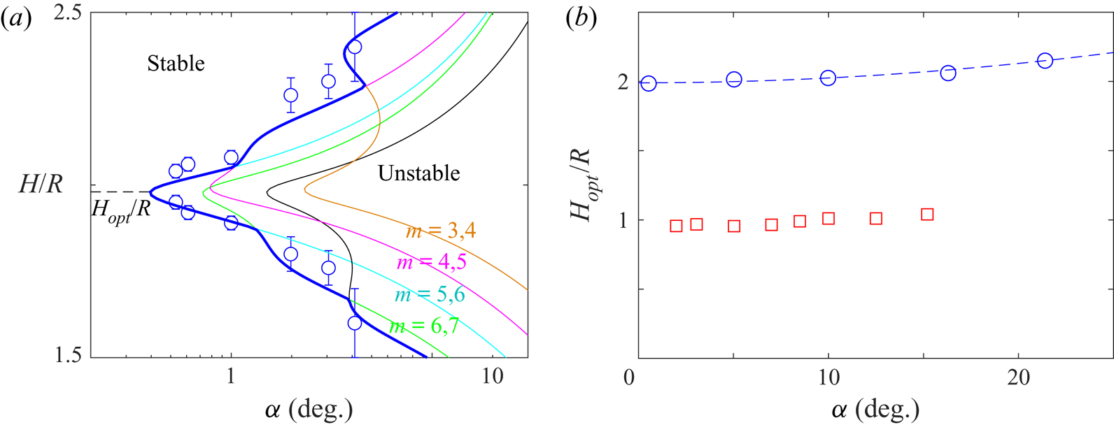
Around the resonance, the amplitude  $a_i$ of the forced Kelvin mode decreases. The instability is less powerful and thus requires a larger tilt angle to remain larger than the dissipation/detuning terms. Figure 5(a) indeed indicates that the instability is only present in a band of aspect ratios around
 $H/R=2$. This unstable band gets larger for larger tilt angles, in very good agreement with the theory. It should be noted that increasing the aspect ratio
 $H/R$ permits to excite modes 4 and 5 (magenta thin line), then modes 3 and 4 (orange thin line). By contrast, decreasing the aspect ratio permits to excite modes 6 and 7 (cyan thin line), then 7 and 8 (green thin line) and so on.
(a) Stability diagram as a function of the aspect ratio  $h$ for a fixed Reynolds number
 $Re=5000$. (b) Optimal aspect ratio at which the flow is the most unstable as a function of the tilt angle for mode 1 (blue
 $\circ$) and mode 2 (red
 $\square$). Symbols correspond to experimental measurements of the threshold. In (a) solid lines correspond to theoretical predictions with no fitting parameter. In (b), the dashed line corresponds to a parabolic fit.

Finally, figure 5(b) indicates that the optimal aspect ratio is almost independent of the tilt angle  $\alpha$. However, there is a very small shift toward larger aspect ratios when
 $\alpha$ increases. This shift seems to scale as
 $\alpha ^2$ and it remains smaller than 8 % for tilt angles up to 20
 $^{\circ }$ degrees.
As noted by Lagrange et al. (Reference Lagrange, Meunier, Nadal and Eloy2011) in the case of a precessing cylinder, the saturation of the instability is mainly due to the presence of a mean retrograde axisymmetric flow. This is visible in the supplementary movies at the end of the linear instability when the vortices with negative (dimensionless) vorticity move toward the centre of the cylinder. The nonlinear model of Lagrange et al. (Reference Lagrange, Meunier, Nadal and Eloy2011) in a precessing cylinder shows that this axisymmetric mode detunes the resonance of the forced Kelvin mode, thus decreasing its amplitude. It leads to a smaller inviscid growth rate which may become smaller than the damping term. This mechanism creates a saturation of the instability close to the threshold and an intermittency of the unstable modes far from the threshold as in the movies of the instability. This intermittency becomes turbulent very far from the threshold.
To conclude, the unsteady flow generated by the instability creates a disorder which increases with the angular velocity and the tilt angle. In the next section, we will show how this chaotic flow can create an efficient mixing.
5. An efficient mixing flow
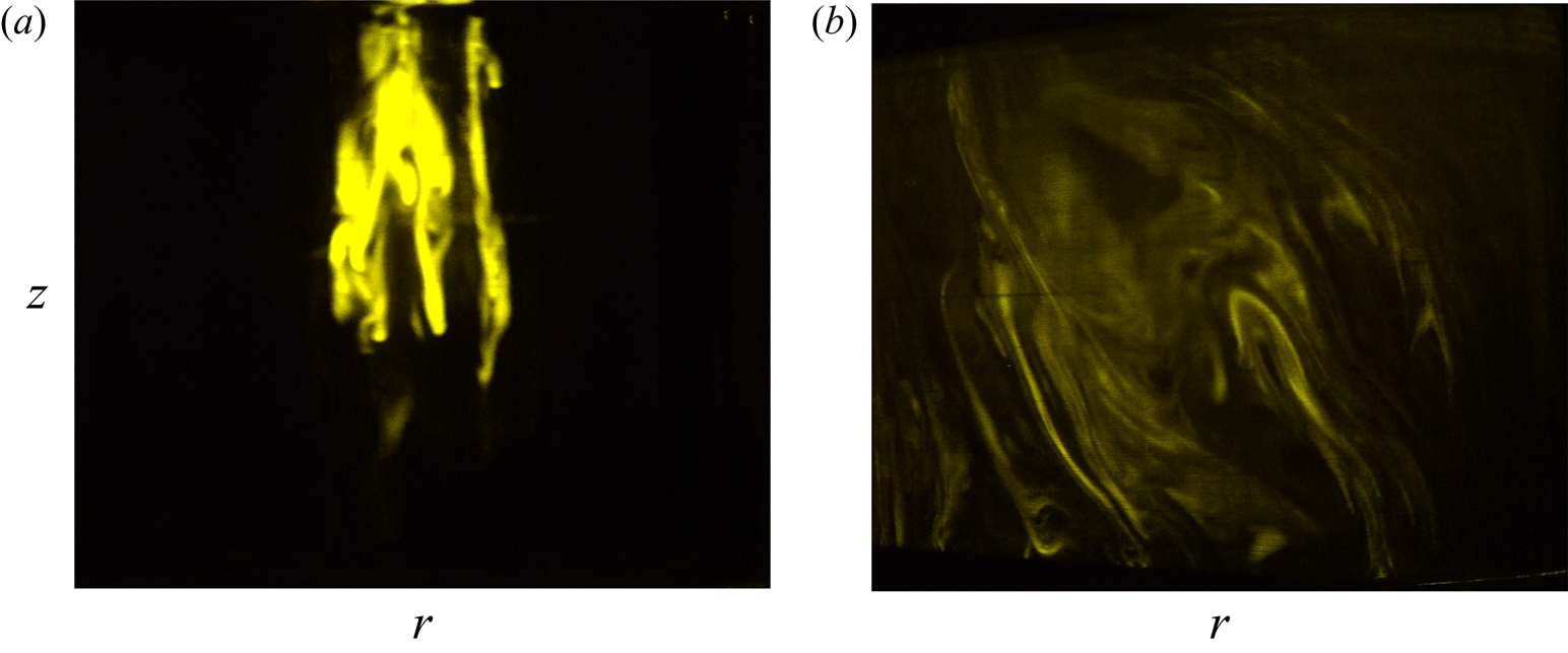
Figure 6(a) shows a visualization of the dye 16 rotation periods after injection for a vertical cylinder ( $\alpha = 0^\circ$). The dye exhibits Taylor columns which are parallel to the axis of rotation of the fluid. These columns remain motionless in the fluid, maintaining strong heterogeneities of dye concentration even at late times. By contrast, figure 6(b) shows the visualization of the dye at the same time for a tilt angle of
 $3^{\circ }$. The dye streaks have been advected by the flow and spread in a much larger portion of the cylinder. The dye streaks are stretched and folded by the instability which is known to create an efficient chaotic mixing. It should be noted that this chaotic advection is only visible in the presence of the instability. Indeed, in the absence of instability, the forced Kelvin mode alone does not generate a strong transport: it simply creates a weak Stokes drift of the dye.
Dye visualizations (a) without tilt and (b) with a tilt angle of  $3^\circ$ at
 $\varOmega t=100$ and
 $Re=10\,000$ in a vertical plane.

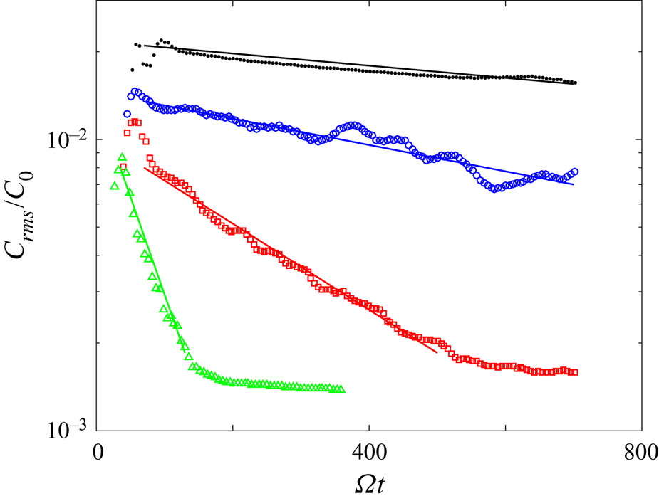
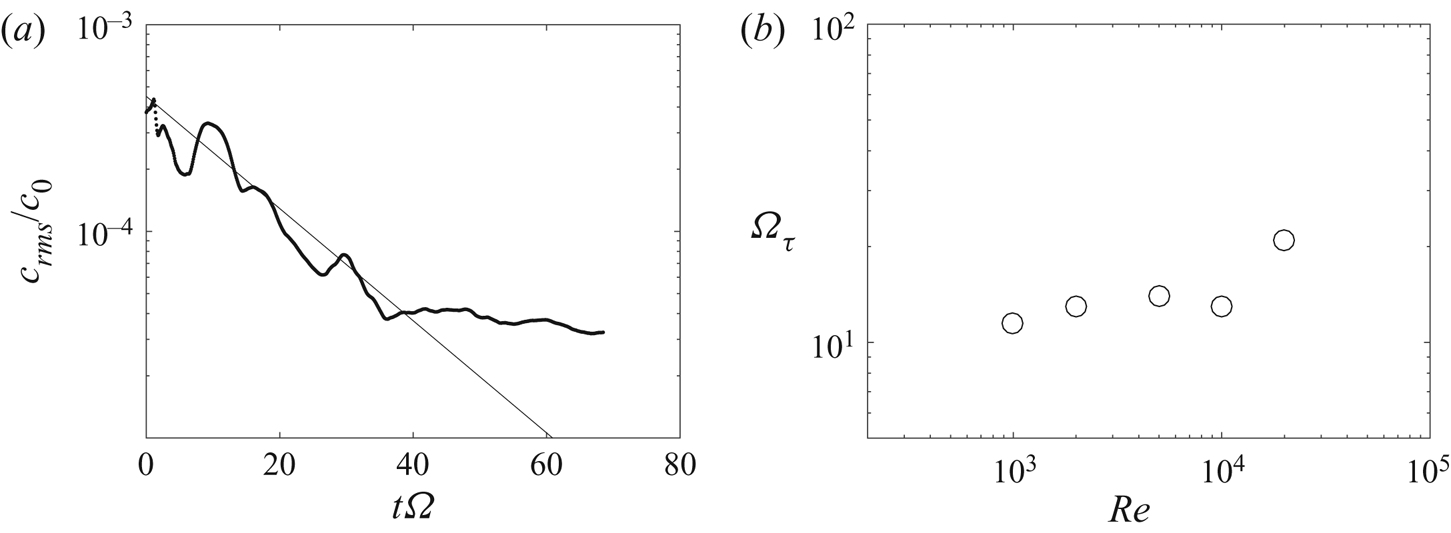
The degree of mixing can be measured quantitatively by plotting the root-mean-square deviation of the concentration field as a function of time. Figure 7 shows that the variance is initially large due to the localized streaks of high concentration (after an initial injection stage which has been partly removed by the temporal filtering of the data). By contrast, when the dye is completely mixed the image is uniform and the variance is thus equal to zero. Figure 7 shows the temporal evolution of the variance for a vertical cylinder compared to tilted cylinders. The variance decreases much faster with a tilt of 10 degrees (red symbols) compared to a vertical cylinder. It proves quantitatively that the mixing is much more efficient for a tilted cylinder.
Variance of the concentration of the dye as a function of time for a tilt angle equal to 0 $^\circ$ (black
 $\bullet$), 1
 $^\circ$ (blue
 $\circ$), 3
 $^\circ$ (red
 $\square$) and 10
 $^\circ$ (green
 $\triangle$). Solid lines correspond to exponential fit.
 ${\textit {Re}}=10\,000$,
 $H/R=2$.

Furthermore, it can be noted that the variance decays exponentially. It can be easily fitted before the saturation (which is due to noise in the images) by  $\textrm {e}^{-t/\tau }$ where the fitting parameter
 $\tau$ corresponds to the characteristic mixing time. An exponential decay of the variance is classical for exponentially stretched layers of dye (Villermaux Reference Villermaux2019). Indeed, if the streak's length increases exponentially as
 $\textrm {e}^{\gamma t}$ (with
 $\gamma$ the stretching rate), the incompressibility imposes initially that its thickness must decrease exponentially as
 $\textrm {e}^{-\gamma t}$ (in the absence of diffusion). This stirring stage does not lead to the decrease of the variance because the maximum of the dye concentration remains unchanged. However, when the thickness reaches the Batchelor scale
 $\sqrt {D/\gamma }$ (where
 $D$ is the diffusivity of the dye), the normal diffusion of dye compensates the convective compression, which leads to a constant thickness of the streak. Consequently, the maximum of concentration must decrease exponentially to conserve the total quantity of dye (Batchelor Reference Batchelor1959). This leads to an exponential decay of the variance.
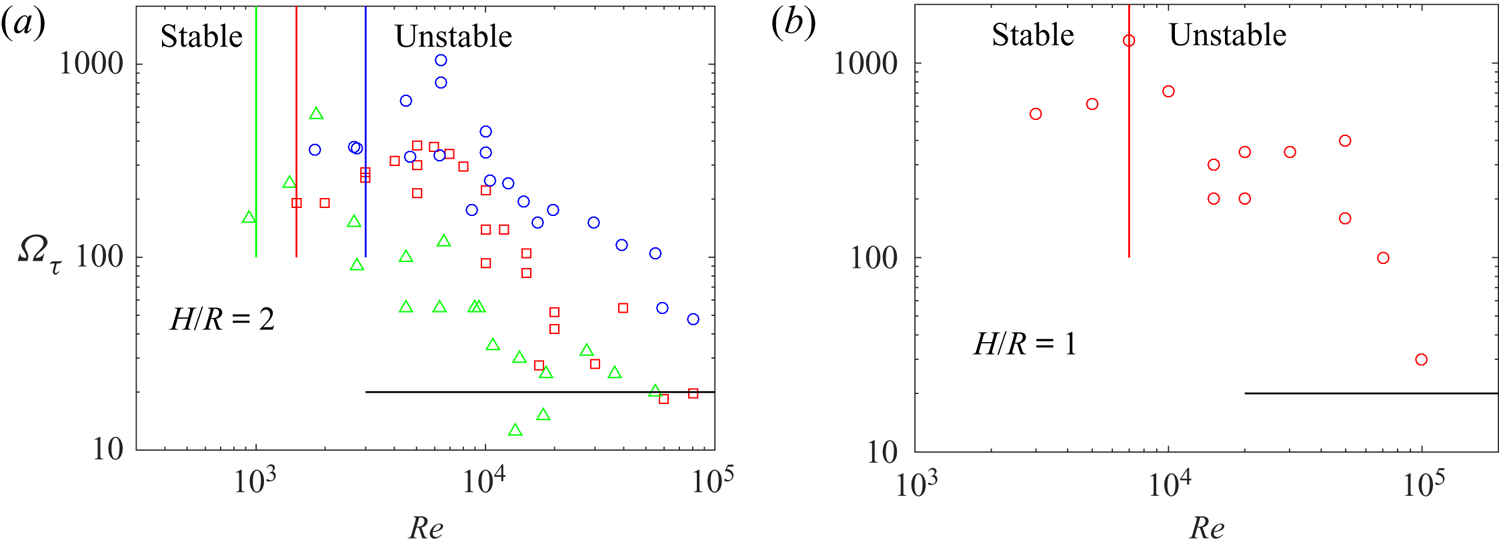
The characteristic mixing times  $\tau$ have been measured for three tilt angles and for Reynolds numbers between 1000 and
 $10^5$. All the experimental results are plotted in figure 8(a) for mode 1 (
 $H/R=2$) and in figure 8(b) for mode 2 (
 $H/R=1$). For small Reynolds numbers, the mixing time
 $\tau$ is very large: it is close to
 $300/\varOmega$, which corresponds to approximately 50 rotation periods. In this regime, the mixing is weak because the forced Kelvin mode is simply a rotating wave. The particles are almost motionless on average, except for a small Stokes drift. Numerical simulations of Lagrangian tracking in a single Kelvin mode (not shown here) have revealed that two particles remain at the same separation distance because they experience the same laminar Stokes drift.
Mixing times  $\tau$ measured for mode 1 (a) and for mode 2 (b) as a function of the Reynolds number. In (a), the tilt angle is equal to 1
 $^\circ$ (blue
 $\circ$), to 3
 $^\circ$ (red
 $\square$) and to 10
 $^\circ$ (green
 $\triangle$). In (b), the tilt angle is equal to 3
 $^\circ$. Coloured solid lines correspond to the threshold at which the flow becomes unstable.

When the Reynolds number increases, the mixing time suddenly drops by a factor 10 and saturates around five rotation periods (plotted as a black solid line in figure 8a). This sudden decrease is due to the instability which creates a complex flow and thus accelerates the mixing of the dye. Indeed, the mixing time starts to decrease when the Reynolds number is approximately three times larger than the Reynolds number at which the instability appears (plotted as coloured solid lines in figure 8a). At large Reynolds numbers, the mixing time of the soft mixer saturates at a value close to  $20/\varOmega$. It means that the variance decreases by a factor
 $e$ in approximately three rotation periods.
A model may be derived using the mixing length theory to predict this sudden decrease of the mixing time. Above the threshold, the characteristic turbulent velocity  $u_t$ of the free Kelvin modes increases from 0 up to a value scaling as
 $\alpha ^{1/4} \varOmega R$ (see Lagrange et al. Reference Lagrange, Meunier, Nadal and Eloy2011, figure 13b). Empirically, this turbulent velocity varies between
 $0.1 \varOmega R$ and
 $0.2 \varOmega R$ for a tilt angle between 1 and
 $10^{\circ }$ at large Reynolds number. The vorticity is of the order of
 $0.5 \varOmega$, which indicates that the size
 $l_t$ of the turbulent structures is of the order of
 $0.3 R$. The turbulent diffusivity
 $D_t = u_t l_t$ is thus expected to increase from 0 at the threshold to
 $0.045 \varOmega R^2$ far from the threshold. Assuming that the diffusive time is of order
 $R^2 /D_t$ leads to a characteristic time which decreases from infinity at threshold down to
 $20/\varOmega$. This is in excellent agreement with the experimental result.
However, this mixing length model should not be used in the stable regime since the forced Kelvin mode alone does not lead to a turbulent diffusivity. If the turbulent velocity and length scales were assumed to be given by  $u_t \sim a_1 u_1 \sim \alpha \sqrt {{\textit {Re}}}$ and
 $l_t \sim R$, the characteristic diffusive time
 $R^2/ (l_t u_t)$ would decrease as
 ${\textit {Re}}^{-1/2}$ and reach a value
 $\tau \sim 1/\varOmega$ for
 $\alpha = 3^\circ$ and
 ${\textit {Re}} \sim 3000$. This is clearly not the case in the experiments: the mixing time
 $\tau$ is two orders of magnitude larger in the stable regime. As noted above, this is due to the fact that the forced Kelvin mode is a simple rotating wave which creates a very weak and laminar transport of the scalar.
The mixing speed of the soft mixer is now compared to the mixing speed of a classical Rushton turbine. A blob of dye is injected in the cylinder with the Rushton turbine and the variance is measured as function of time. Figure 9(a) indicates that the variance decreases exponentially during one decade until saturation due to the inhomogeneities of the laser sheet. Fitting this decay with a law of the form  $\textrm {e}^{-t/\tau }$ gives the mixing time for each experiment. The mixing time is plotted as a function of the Reynolds number in figure 9(b) over more than a decade. It seems to be nearly independent of the Reynolds number in the range
 $10/\varOmega$ to
 $20/\varOmega$. It means that the variance decreases by
 $e$ in about two to three rotation periods. This is in good agreement with the result given by Nagata (Reference Nagata1975) who found that the mixing time is close to five rotation periods at large Reynolds number. A mixing length model may be used with a characteristic turbulent velocity
 $u_t \sim \varOmega R$ and a characteristic length scale
 $l_t \sim 0.1 R$ leading to a characteristic mixing time of the order of
 $10/\varOmega$.
(a) Variance of the dye concentration as a function of time for a Rushton turbine at a Reynolds number (based on the cylinder's radius) equal to  ${\textit {Re}}=15\,000$. Experimental measurements (symbols) are fitted by an exponential law of the form
 $\text{e}^{-t/\tau }$ (solid line). (b) Mixing times
 $\tau$ as a function of the Reynolds number.

6. A low-shear flow
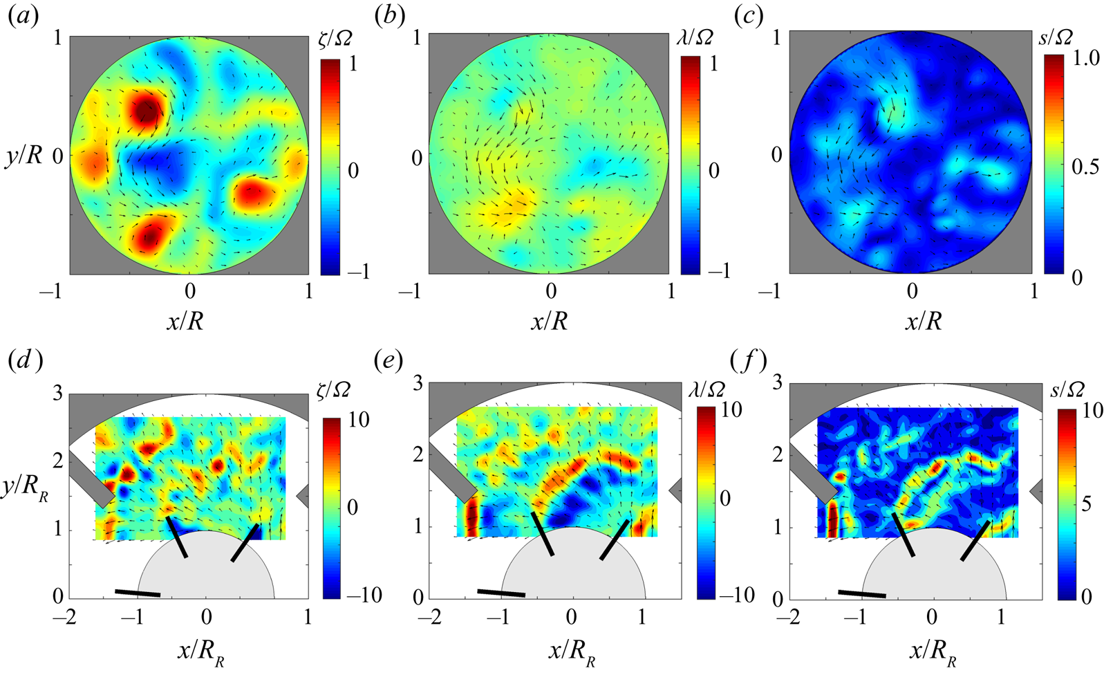
In the previous section, we have shown that the flow inside the soft mixer is as efficient as a Rushton turbine to mix a passive scalar for the same rotation speed. In this section, we will compare the velocity gradients obtained in a soft mixer and in a Rushton turbine flow. The vorticity measured at mid-height of the soft mixer is shown in figure 10(a) for a large Reynolds number ( $Re=20\,000$) and a tilt angle of
 $3^\circ$, i.e. in the fast mixing regime. It exhibits several positive and negative vortices of moderate size (with radius
 $l_t$ equal to approximately
 $R/3$). The axial vorticity is of the order of the angular velocity
 $\varOmega$. By contrast, figure 10(d) shows the vorticity created by a Rushton turbine. The vorticity is 10 times larger than in the soft mixer (note the change in the colour scale). The vortices are smaller (radius
 $l_t$ of the order of
 $R/10$) which partly explains why the vorticity is larger (since it scales as
 $u_t/l_t$).
Comparison of the flow created by a soft mixer (rotating outer cylinder) and by a Rushton turbine (motionless outer cylinder and inner disk of radius  $R$ with vertical blades rotating at
 $\varOmega$). The velocity fields are measured by PIV at mid-height for the soft mixer and at the altitude of the disk for the Rushton turbine. For the soft mixer, the Reynolds number is equal to
 $Re=\varOmega R^2/\nu =20\,000$ and the tilt angle is equal to 3
 $^\circ$ which corresponds to the efficient mixing regime. For the Rushton turbine, the cylinder's based Reynolds number is equal to
 $Re=\varOmega R^2/\nu =15\,000$ and the turbine's based Reynolds number is equal to
 $Re_R=\varOmega R_R^2/\nu =5000$. Note the change in colour scale between the two flows.

The horizontal divergence of the flow  $\lambda =\partial u/\partial x + \partial v/\partial y$ has also been measured for the soft mixer (figure 10b) and the Rushton turbine (figure 10e). The contrast between the two flows is even more pronounced. The Rushton turbine creates a divergence
 $\lambda$ which is approximately 20 times larger than for the soft mixer. This strong divergence is emitted at the tip of the rotating blades (plotted in black). It is of the order of ten times the angular velocity
 $\varOmega$. By contrast, the divergence in the soft mixer is only equal to half the angular velocity
 $\varOmega$.
Finally, the shear is also measured and compared between the two flows (figure 10c,f). It is quantified by the strain  $s$, defined as the largest eigenvalue of the symmetric velocity gradient tensor. As mentioned before, the strain is much larger in the Rushton turbine mixer than for in the soft mixer. It is of the order of 30 % of the angular velocity
 $\varOmega$ for the soft mixer whereas it is equal to approximately
 $10\varOmega$ for the Rushton turbine.
It means that for the same mixing time (equal to approximately  $15/ \varOmega$ for both set-ups), the soft mixer has a strain approximately 30 times smaller than the Rushton turbine. Alternatively, it means that for a flow with the same strain (and thus an angular velocity 30 times larger for the soft mixer), the mixing time is 30 times faster than for the Rushton turbine.
The low shear found in the soft mixer is a direct consequence of the presence of large-scale structures which create a strong mixing while minimizing the velocity gradients. Indeed, the mixing length model indicates that the characteristic mixing time scales as  $\tau \sim R^2/(l_t u_t) \sim (R/l_t)^2/s_t$ where
 $s_t$ corresponds to the shear of the turbulent structures. For equivalent mixing times, the shear is thus nine times larger if the turbulent eddies are three times smaller.
The low-shear flow observed in a soft mixer is thus of high interest for biological applications since many cells and micro-organisms are very sensitive to the strain. Such a high mixing and low-shear flow is thus an ideal candidate for a bioreactor.
7. Conclusions
The flow inside a soft mixer has been characterized by means of visualizations and velocity measurements. The set-up consists in a cylinder rotating around its axis which is tilted at a small angle with respect to the vertical. The free surface, which remains horizontal, excites inertial modes in the bulk of the fluid. The first inertial mode becomes resonant when the height of fluid is equal to twice the radius, leading to a turbulent flow via a parametric instability (also called triadic resonance) at larger Reynolds numbers. The viscous threshold of the instability predicted analytically with no adjustable parameter is in excellent agreement with the experimental results. This unstable flow strongly accelerates the mixing of a passive scalar, as measured quantitatively using laser induced fluorescence. The characteristic mixing time is equal to approximately five rotation periods of the cylinder at large Reynolds numbers. This value is very close to the value measured in a mixer with a Rushton turbine. Nevertheless, the shear measured in a soft mixer is 20 to 30 times smaller than in a mixer with a Rushton turbine.
The low shear and the efficient mixing of the flow inside the soft mixer is extremely interesting for different applications. First, it can help designing geoinspired bioreactors for the growth of fragile cells such as stem cells. Our preliminary results have been obtained with micro algae sensitive to the shear (dinoflagellates). The duplication growth rate was found to be an order of magnitude larger than in the absence of motion. It proves that the mixing is sufficiently effective to provide the algae with enough carbon dioxide, while maintaining a low shear rate. Further applications with different cells are required in order to verify that this set-up can be used as an efficient bioreactor. Second, this soft mixer can be useful to mix large volumes of viscous fluids. Indeed, the mixing in a soft mixer is very homogeneous within the container. It does not create unmixed zones which are often observed while using a Rushton turbine. Furthermore, the power required to rotate the soft mixer is much smaller than the power needed for a Rushton turbine. Indeed, the energy is injected at large scale rather than at small scale (i.e. behind the blades of the Rushton turbine). The viscous dissipation is thus much smaller. All these aspects indicate that this patented soft mixer (Meunier & Manasseh Reference Meunier and Manasseh2017) could lead to a new generation of mixers for biological and industrial applications.
Finally, this simple set-up is also very interesting for fundamental studies on precessing flows. Indeed, the simplicity of the mechanical device would make it possible to reach very large Reynolds numbers (i.e. very small Ekman numbers) with a very small forcing. Measuring turbulent velocity fields and spectra is also easier for this flow than inside a precessing cylinder since there is a single axis of rotation instead of two. This experiment thus seems to provide a good idealized flow for the study or rotating turbulence.
Acknowledgements
The author would like to thank Dr C. Barbosa and Dr C. Nobili for preliminary results and A. Duchene and P. Fruton for technical help in getting the final results. The financial support of SATT Sud Est and of Labex Mec is also gratefully acknowledged.
Declaration of interests
The author reports no conflict of interest.
Supplementary movies
Supplementary movies are available at https://doi.org/10.1017/jfm.2020.634.
Appendix A
A.1. Viscous base flow at the resonance
As shown in § 3, the inviscid amplitude  $a_i$ of a Kelvin mode diverges when the height of fluid corresponds to a multiple of its half wavelength
 ${\rm \pi} /k_i$ due to the vanishing denominator
 $\sin (k_i h)$ in (3.10). Viscous effects saturate the inviscid amplitude such that Ekman pumping and volumic attenuation must be taken into account. The viscous amplitude can be obtained for example by deriving a solubility condition. This condition is obtained by multiplying the Navier Stokes equations by the complex conjugate of the Kelvin mode
 $[\overline {u^r_i} \cos (k_i z),\overline {u^\theta _i} \cos (k_i z),\overline {u^z_i} \sin (k_i z)]$ and by integrating over the volume of the cylinder excluding the Ekman boundary layers, which leads to
 \begin{equation} \iint \overline{p_i} \boldsymbol{u} \boldsymbol{\cdot} \boldsymbol{n} \,\textrm{d} S + \iint p \overline{\boldsymbol{u}_i} \boldsymbol{\cdot} \boldsymbol{n} \,\textrm{d} S + \nu \iiint \overline{\boldsymbol{u}_i} \boldsymbol{\cdot} {\rm \Delta} \boldsymbol{u} \,\textrm{d} V = 0, \end{equation}
where  $\bar {\boldsymbol{\cdot} }$ is the complex conjugate. This equation is then divided by
 $\varOmega ^2 R^4$ in order to reach non-dimensional coefficients. At the free surface, the true velocity
 $\boldsymbol {u}$ is given by the boundary condition (3.9) such that the first term integrated over the free surface leads to the forcing term
 $- \alpha \varOmega R F$ with
 \begin{equation} F = 2j {\rm \pi} \cos(k_i H) \frac{1}{R^3} \int_0^R r^2 \,\textrm{J}_1(\sqrt{3}k_i r)\,\textrm{d} r. \end{equation}
The integral of the second term over the free surface can be calculated by replacing the true velocity  $\boldsymbol {u}$ from (3.4), leading to a term
 $a_i \sin (k_i H) T$ with
 \begin{equation} T=2 j {\rm \pi} \cos(k_i H) \frac{1}{R^2} \int_0^R \textrm{J}_1^2(\sqrt{3}k_i r)r\,\textrm{d} r. \end{equation}
The integral of the second term at the bottom and at the periphery vanish at the resonance because the Kelvin modes have no normal velocity. But the surface integral of the first term does not vanish at the bottom and at the periphery because the surface integrals are taken outside of the Ekman layers. The true normal velocity  $\boldsymbol {u}$ is thus equal to the Ekman pumping, which can be calculated using a classical boundary layer analysis (see Meunier et al. Reference Meunier, Eloy, Lagrange and Nadal2008). Assuming that the horizontal velocity
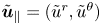 $\tilde {\boldsymbol {u}}_{\parallel }=(\tilde {u}^r,\tilde {u}^\theta )$ depends on a rescaled vertical coordinate
 $\tilde {z}=z \sqrt {{\textit {Re}}}$, the Navier–Stokes equations become inside the Ekman layer
 \begin{equation} j \tilde{\boldsymbol{u}}_{\parallel}+ 2 \varOmega \hat{\textbf{z}} \times \tilde{\boldsymbol{u}}_{\parallel} - \frac{\partial^2 \tilde{\boldsymbol{u}}_{\parallel}}{\partial \tilde{z}^2} = 0 \end{equation}
subject to the boundary conditions
 \begin{gather} \tilde{\boldsymbol{u}}_{\parallel} (\tilde{z}=+\infty) = \frac{a_i}{k_i} \left(\begin{array}{l} u^r_i(r) \\ u^\theta_i(r) \end{array} \right) \exp({j(\theta+\varOmega t)}), \end{gather}
 \begin{gather}\tilde{\boldsymbol{u}}_{\parallel} (\tilde{z}=0) = 0, \end{gather}
where  $u^r_i(r)$ and
 $u^\theta _i(r)$ are given in (3.5). The solution is given by
 \begin{gather} \tilde{\boldsymbol{u}}_{\parallel}^r = [\,jS(r)\,\textrm{e}^{-\kappa_S \tilde{z}} -jD(r)\,\textrm{e}^{-\kappa_D \tilde{z}} + u_i^r] \frac{a_i}{k_i}\exp({\,j(\theta+\varOmega t)}) \end{gather}
 \begin{gather}\tilde{\boldsymbol{u}}_{\parallel}^\theta = [S(r)\,\textrm{e}^{-\kappa_S \tilde{z}} +D(r)\,\textrm{e}^{-\kappa_D \tilde{z}} + u_i^\theta] \frac{a_i}{k_i}\exp({\,j(\theta+\varOmega t)}) \end{gather}
with
 \begin{gather} \kappa_S=(1+j)\sqrt{3}/2, \end{gather}
 \begin{gather}\kappa_D=(1-j)/\sqrt{2}, \end{gather}
 \begin{gather}S(r)=(i u_i^r -u_i^\theta)/2, \end{gather}
 \begin{gather}D(r)=-(i u_i^r +u_i^\theta)/2. \end{gather}
Integration of the incompressibility from  $\tilde {z}=0$ to
 $+\infty$ gives the value of the normal velocity outside of the Ekman layer (at
 $\tilde {z}=+\infty$)
 \begin{equation} \tilde{\boldsymbol{u}}^z = {\textit{Re}}^{-1/2} \left[\frac{-j D'(r)}{\kappa_D} + \frac{j(S'(r)+2S(r)/r)}{\kappa_S} \right] \frac{a_i}{k_i} \exp({\,j(\theta+\varOmega t)}). \end{equation}
Integrating this formula over the bottom leads to a term  $a_i B / \sqrt {{\textit {Re}}}$ in (A 1) with
 \begin{equation} B= \frac{6 {\rm \pi} k_i}{R} \left(\frac{1-j}{2\sqrt{2}}+\frac{1+j}{6\sqrt{6}}\right) \int_{0}^{R}\textrm{J}_1^2(\sqrt{3}k_i r)r\,\textrm{d} r, \end{equation}
for the bottom Ekman layer. A similar calculation at the periphery of the cylinder gives a term  $a_i C /\sqrt {{\textit {Re}}}$ with
 \begin{equation} C= \frac{{\rm \pi} H }{k_i R^2} \frac{1+j}{\sqrt{2}} (1+k_i^2 R^2) \textrm{J}_1^2(\sqrt{3} k_i R) \left[ 1-\frac{\sin(2k_iH)}{2k_iH}\right], \end{equation}
for the Ekman layer on the side of the cylinder. Finally, the triple integral over the volume corresponds to the volumic viscous effects and lead to a term  $a_i V / {\textit {Re}}$ with
 \begin{equation} V= \frac{8{\rm \pi} H k_i}{3} \textrm{J}_1^2(\sqrt{3}k_i R) \left[1+2k_i^2 R^2+\frac{\sin(k_i H)}{2 k_i H}(1-k_i^2 R^2) \right]. \end{equation}
Assuming that the sum of these five terms vanishes leads to the viscous amplitude of the forced Kelvin mode
 \begin{equation} a_i=\frac{F/T}{-\sin(k_i H) + (B+C)/(T\sqrt{{\textit{Re}}}) + V/(T {\textit{Re}})} \alpha \varOmega R .\end{equation}
Outside of the resonance, the terms containing  ${\textit {Re}}$ are negligible at large Reynolds number such that this equation simplifies into (3.10). At the resonance,
 $\sin (k_i H)$ vanishes such that the viscous terms become dominant. The amplitude
 $a_i$ is thus given by (3.13) if the volumic viscous term is neglected.
A.2. Parametric instability by triadic resonance
At the resonance of the  $i$th forced Kelvin mode
 $\boldsymbol {u}_i$, the amplitude
 $a_i$ is larger than the amplitudes of the other forced Kelvin modes because its amplitude scales as
 $\alpha \sqrt {{\textit {Re}}}$ whereas the non-resonant forced mode amplitudes scale as
 $\alpha$. For tilt angles smaller than
 $1/\sqrt {{\textit {Re}}}$ the amplitude
 $a_i$ constitutes a small parameter. Two free Kelvin modes are added with a small amplitude growing slowly in time (Lagrange et al. Reference Lagrange, Meunier, Nadal and Eloy2011). The velocity is thus searched as
 \begin{align} \boldsymbol{u} &=
\frac{a_i}{4 k_i R} \boldsymbol{u}_i \exp({\,j(\pm k_i z +
\theta + \varOmega t)}) + a' \boldsymbol{u}' \exp({\,j(\pm k'
z + m' \theta + \omega' t)}) \nonumber\\ &\quad + a''
\boldsymbol{u}'' \exp({\,j(\pm k'' z + m'' \theta + \omega''
t)}) +\mathrm{c.c.}, \end{align}
where c.c. corresponds to the complex conjugate and where  $\pm k$ indicates that the term with a positive wavenumber must be added to the same term with a negative wavenumber. The first term corresponds to the resonant Kelvin mode given in (3.4). The wavenumbers
 $k'$ and
 $k''$ of the second and third terms must be multiples of
 ${\rm \pi} /H$ in order for the free modes to respect the boundary conditions at the top and bottom. The radial structure of the free mode
 $\boldsymbol {u}'$ is given by
 \begin{equation} \boldsymbol{u}' =
\left( {\begin{array}{@{}c@{}} \dfrac{{ \varOmega^2}}{{4
\varOmega^2 - \omega'^2 }}\left( \omega' \delta' R J_{m'
}^{\prime} \left( {\delta' r} \right)/\varOmega +
2\dfrac{{m'R}}{r}J_{m' } \left( {\delta' r} \right) \right)
\\ \dfrac{{ j\varOmega^2}}{{4\varOmega^2
- \omega'^2 }}\left( {2\delta' R J_{m' }^{\prime} \left(
{\delta' r} \right) + \dfrac{{\omega' m' R}}{\varOmega
r}J_{m' } \left( {\delta' r} \right)} \right)
\\ - j \dfrac{{k' R \varOmega}}{{\omega'
}}J_{m' } \left( {\delta' r} \right)
\end{array}} \right),
\end{equation}
with the radial wavenumber given by  $\delta '=|k'| \sqrt {4\varOmega ^2/\omega '^2-1}$. The frequency
 $\omega '$ is given by the dispersion relation of the Kelvin modes
 $u'$ (to respect the boundary conditions
 $u^r=0$ at
 $r=R$)
 \begin{equation} \frac{\omega'}{\varOmega} \delta' J_{m' }^{\prime} \left( {\delta'} \right) + 2 m' J_{m'} \left( {\delta'} \right) = 0. \end{equation}
The radial structure of mode  $\boldsymbol {u}''$ and its corresponding dispersion relation are given by the same equations replacing
 $'$ by
 $''$.
If the three resonance conditions
 \begin{equation} \left.\begin{array}{@{}c@{}} |k''-k'|=k_i \\ m''-m'=1 \\ \omega''-\omega'=\varOmega \end{array}\right\} \end{equation}
are satisfied, the nonlinear interaction of the forced mode  $\boldsymbol {u}_i$ and the free mode
 $\boldsymbol {u}'$ can force the temporal derivative of the second free mode
 $\boldsymbol {u}''$ because they have the same Fourier component. Due to the presence of the complex conjugates, the same mechanism occurs for the temporal derivative of the first free mode
 $\boldsymbol {u}'$. Assuming that the amplitude
 $a'$ is slowly varying in time, the amplitude equation for the first mode can be calculated by introducing the decomposition (A 18) into the Navier–Stokes equation, by multiplying with the complex conjugate of
 $r \boldsymbol {u}' \exp ({\,j(k' z + m' \theta + \omega ' t)})$ and by integrating over the volume of the cylinder, leading to
 \begin{equation} \frac{\partial a'}{\partial t} = N' a'' \frac{\overline{a_i}}{4 k_i R^2 \varOmega} - \frac{S' a'}{\sqrt{{\textit{Re}}}} - \frac{V' a'}{{\textit{Re}}} - j Q' {\rm \Delta} k' a'. \end{equation}
A similar amplitude equation can be found for mode  $\boldsymbol {u}''$:
 \begin{equation} \frac{\partial a''}{\partial t} = N'' a' \frac{a_i}{4 k_i R^2 \varOmega} - \frac{S'' a''}{\sqrt{{\textit{Re}}}} - \frac{V'' a''}{{\textit{Re}}} - j Q'' {\rm \Delta} k'' a''. \end{equation}
The coefficients are given analytically (see appendix B of Lagrange et al. Reference Lagrange, Meunier, Nadal and Eloy2011)
 \begin{gather} N' = -2R \left( \pm k_i - k''\frac{ \varOmega}{\omega'' } \right) \frac{\displaystyle\int_0^R {\left| \boldsymbol{u}_i, \ \boldsymbol{u}', \ \overline{\boldsymbol{u}''} \right|r\,\textrm{d} r}}{\displaystyle\int_0^R |\boldsymbol{u}'|^2 r\,\textrm{d} r}, \end{gather}
 \begin{gather}N'' = 2R \left( \pm k_i - k'\frac{ \varOmega}{\omega' } \right) \frac{\displaystyle\int_0^R {\left| \boldsymbol{u}_i, \ \boldsymbol{u}', \ \overline{\boldsymbol{u}''} \right|rdr}}{\displaystyle\int_0^R |\boldsymbol{u}''|^2 rdr}, \end{gather}
where the operator  $| \cdot ,\cdot ,\cdot |$ is the determinant. The
 $\pm$ sign is equal to
 $+$ if
 $k'' -k' =k$ and equal to
 $-$ if
 $k' -k'' =k$. For example, for
 $H/R=1.94$, the resonance conditions are exactly met for
 $m'=5$ and
 $m''=6$. Indeed, for a wavenumber equal to
 $k'={\rm \pi} /H$, the frequency given by the dispersion relation (A 20) is equal to
 $\omega '=-0.35\varOmega$. If the wavenumber
 $k''$ is equal to
 $2 {\rm \pi} /H$, the frequency
 $\omega ''$ is equal to
 $0.65 \varOmega$, such that the difference
 $\omega ''-\omega '$ is equal to
 $\varOmega$. In that case, the nonlinear coefficients can be calculated to be
 $N'=-1.28$ and
 $N''=-1.96$.
The surface viscous coefficients are adapted from Lagrange et al. (Reference Lagrange, Meunier, Nadal and Eloy2011) by assuming that the free surface does not create any Ekman pumping. The coefficient  $I'^z$ corresponding to Ekman pumping at the bottom is not taken into account twice as in the case of precession. This leads to
 \begin{equation} S' = R^3 \frac{2 I'^r + I'^z }{4 {\rm \pi} H \int_0^R |\boldsymbol{u}'|^2 r\,\textrm{d} r}, \end{equation}
with
 \begin{align} I'^r &= \frac{ \sqrt{8} {\rm \pi} H J_{m'}(\delta'R)\sqrt{|\varOmega/\omega'|} } {R[\mathrm{sign}(\omega'/\varOmega)-j]} \nonumber\\ &\quad \times\left[\left(\frac{\varOmega k'^2R^2}{\omega'}- \frac{m'^2\omega'\varOmega}{4\varOmega^2-\omega'^2}\right)J_{m'}(\delta'R) -\frac{2 m' \delta' R\varOmega^2}{4\varOmega^2-\omega'^2}J'_{m'}(\delta'R) \right] \end{align}
 \begin{align} I'^z &= \frac{\sqrt{2}{\rm \pi}(1-j)J_{m'}^2(\delta'R)}{(\omega'/\varOmega)^2} \left[ \frac{(\delta'^2R^2-m'^2) \omega'^2}{\varOmega^2} + 4m'^2 \right]\nonumber\\ &\quad \times\left[ \frac{1}{(2-\omega'/\varOmega)^{3/2}}+\frac{j}{(2+\omega'/\varOmega)^{3/2}}\right]. \end{align}
The surface dissipation coefficient  $S''$ is simply obtained by replacing primes by double primes. For example, for
 $m'=5$ and
 $m''=6$, the viscous coefficients are found to be
 $S'=0.89-0.26j$ and
 $S''=1.06 + 0.29j$.
The volume viscous coefficient is simply given by
 \begin{equation} V'= (k'^2 + \delta'^2) R^2. \end{equation}
Numerically, for  $m'=5$ and
 $m''=6$, it is found that
 $V'=85$ and
 $V''=99$.
The detuning parameter  $Q' R {\rm \Delta} k'$ is obtained from
 \begin{equation} Q' = \frac{-2 k' R \varOmega \int_0^R J_{m'}^2(\delta'R) r\,\textrm{d} r }{\omega' \int_0^R |\boldsymbol{u}'|^2 r\,\textrm{d} r}, \end{equation}
and  ${\rm \Delta} k'$ given by the opposite of the difference between the wavenumber
 $k'$ and the nearest multiple of
 ${\rm \pi} /H$ (see (4.10) of Lagrange et al. Reference Lagrange, Meunier, Nadal and Eloy2011). Numerically, it is found for
 $m'=5$ and
 $m''=6$ that
 $Q'=0.204$ and
 $Q''=-0.187$.
The two amplitude equations (A 22) and (A 23) can be solved, leading to an exponential growth of both modes as  $\textrm {e}^{\sigma t}$ with a growth rate
 $\sigma$ solution of
 \begin{equation} \left( \frac{\sigma}{\varOmega} + D' \right)\left( \frac{\sigma}{\varOmega} + D'' \right)= \frac{N'N'' |a_i|^2}{16 k_i^2 R^4 \varOmega^2}, \end{equation}
where the dissipation/detuning terms  $D'$ and
 $D''$ are defined as
 \begin{equation} \left.\begin{gathered} D' = \frac{S'}{\sqrt{{\textit{Re}}}} + \frac{V'}{{\textit{Re}}} + j Q' {\rm \Delta} k', \\ D'' = \frac{S''}{\sqrt{{\textit{Re}}}} + \frac{V''}{{\textit{Re}}} + j Q'' {\rm \Delta} k''. \end{gathered}\right\} \end{equation}
For large Reynolds numbers and in the absence of detuning, the inviscid growth rate simplifies into (4.8). In the presence of all dissipation/detuning terms, the critical amplitude  $a_i$ at which the flow destabilizes can be calculated by assuming that the real part of the growth rate vanishes, i.e. that the growth rate is purely imaginary, leading to (Lagrange et al. Reference Lagrange, Meunier, Nadal and Eloy2011)
 \begin{equation} |a_i| = 4 k_i R \left\{ \frac{\textrm{Re}(D')\textrm{Re}(D'')}{N'N''} \left[ 1+ \frac{{\rm Im}(D'-D'')^2}{\textrm{Re}(D'+D'')^2} \right] \right\}^{1/2} \varOmega R, \end{equation}
where  ${\rm Im}$ is the imaginary part. Equating this equation with the modulus of (A 17) gives the value of the critical angle
 $\alpha$ at which the flow becomes unstable:
 \begin{align} \alpha = \frac{4 k_i R}{|F|} \left\{ \frac{\textrm{Re}(D')\textrm{Re}(D'')}{N'N''} \left[ 1+ \frac{{\rm Im}(D'-D'')^2}{\textrm{Re}(D'+D'')^2} \right] \right\}^{1/2} \left| -T \sin(k_i H) + \frac{B+C}{\sqrt{{\textit{Re}}}} + \frac{V}{{\textit{Re}}} \right|. \end{align}
This threshold is plotted in figure 4(a) at  $H/R=2$ (blue) for the first resonance of mode 1 and at
 $H/R=1$ (red) for the first resonance of mode 2. It is also plotted in figure 5(a) at
 ${\textit {Re}}=5000$.