1 Introduction
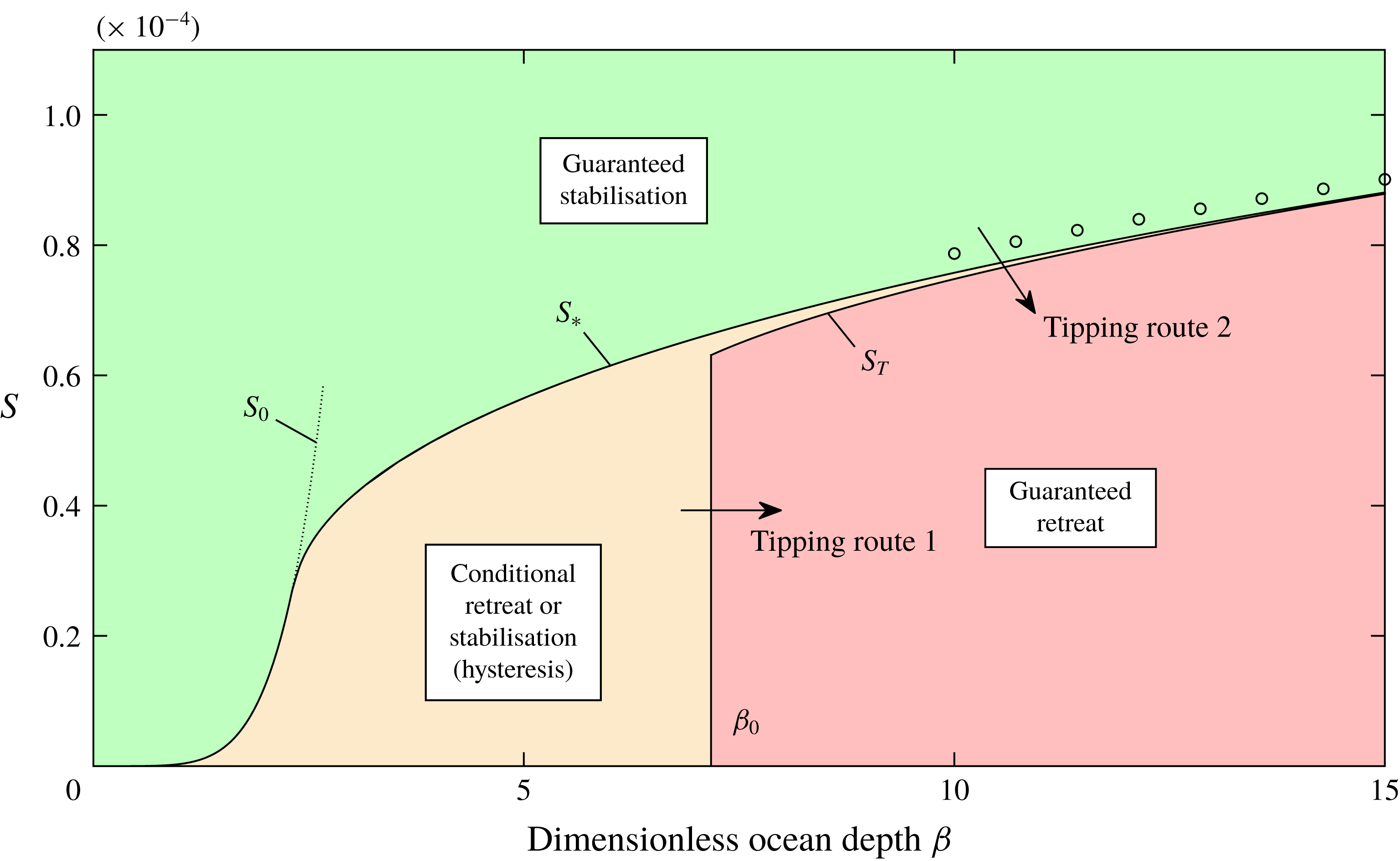
The total or partial collapse of the West Antarctic Ice Sheet (WAIS) – the largest example of a so-called marine ice sheet – has the potential to increase global sea level independently by several metres over the course of the next few centuries (Bamber et al. Reference Bamber, Riva, Vermeersen and LeBrocq2009; Hanna et al. Reference Hanna2013). However, the conditions controlling its destabilisation are currently poorly understood. A marine ice sheet is a continent-scale glacial mass whose base lies submerged in the ocean. Since ice is lighter than water, buoyancy acts to detach a marine ice sheet from the underlying bedrock. This has led to a long-standing open problem in glaciology regarding the conditions under which buoyancy drives a marine ice sheet to collapse, a principle known as the ‘marine ice sheet instability’ (MISI) (Weertman Reference Weertman1974; Thomas & Bentley Reference Thomas and Bentley1978). The essential likelihood of instability, and the mode and time scales on which it may be triggered, remain key unknowns in efforts to assess contributions to future sea-level rise. A potentially key mechanism for suppressing MISI is an effect of the peripheral floating regions of the ice sheet (the ice shelves) in creating a buttress that supports the considerably larger grounded interior of the ice sheet against surging outwards into the ocean (Hughes Reference Hughes1981; Stuiver et al. Reference Stuiver, Denton, Hughes and Fastook1981). The process of ice-shelf buttressing may be key to understanding marine ice sheet collapse, providing a strong motivation to explore its mechanical underpinnings. The present paper presents a theoretical investigation of the mechanisms by which the onset of, suppression of and recovery from MISI is controlled by lateral stresses and ice-shelf buttressing. A focus is to demonstrate parametric tipping points for triggering of a large-scale retreat occurring once the conditions for sustaining a stable steady state fail critically.
In describing the onset of MISI, I distinguish two different modes of grounding-line retreat. Following changes in external parametric conditions (e.g. a reduction in snow accumulation rate or an increase in the rate of melting of the ice shelf), a grounding line may retreat towards a new stable steady state near the present grounding line. In this mode of ‘stable’ retreat, the grounding line will recover to its original position if parameters are subsequently restored to their former values. If the changing external conditions instead lead to a removal of the possibility of a stable steady state near the present state, then a more sudden and sustained retreat can instigate from which recovery may be impossible following even complete parametric restoration. The onset of this mode of ‘tipped’ retreat is identified with the notion of MISI.
The main analytical tool I use is the steady-state balance equation for the grounding-line position
 $x_{G}$
(Pegler Reference Pegler2018),
 $$\begin{eqnarray}E[d(x_{G})]+B(x_{G},x_{C})={\textstyle \frac{1}{2}}\unicode[STIX]{x1D70C}g^{\prime }d(x_{G})^{2},\end{eqnarray}$$
where
 $d(x)$
is the flotation profile (related to the bed profile),
 $E$
is a function representing the depth-integrated longitudinal extensional stress in steady state,
 $B$
is a function representing the ice-shelf buttressing force in steady state,
 $x_{C}$
is the calving position of the ice shelf,
 $\unicode[STIX]{x1D70C}$
is the density and
 $g^{\prime }$
is the reduced gravity. The functions
 $E[d(x_{G})]$
and
 $B(x_{G},x_{C})$
represent universal analytical functions of the grounding-line position
 $x_{G}$
that are derived from integrations of the grounded and floating components of a quasi-two-dimensional (Q2D) model (to be reviewed in § 2). The Q2D model is defined as a flow-line model (Dupont & Alley Reference Dupont and Alley2005; Nick et al.
Reference Nick, van der Veen, Vieli and Benn2010; Hindmarsh Reference Hindmarsh2012; Pegler et al.
Reference Pegler, Kowal, Hasenclever and Worster2013; Walker et al.
Reference Walker, Holland, Parizek, Alley, Nowicki and Jenkins2013; Kowal, Pegler & Worster Reference Kowal, Pegler and Worster2016; Pegler Reference Pegler2016; Schoof, Davis & Popa Reference Schoof, Davis and Popa2017) with use of a parametrisation of the transverse viscous shear stress for hard margins (Pegler Reference Pegler2016). The algebraic equation (1.1) determines the steady-state grounding-line positions considerably faster than numerical analysis based on the full two-dimensional shallow stream/shelf equations (SSA) (e.g. Gudmundsson et al.
Reference Gudmundsson, Krug, Durand, Favier and Gagliardini2012), but nonetheless recovers its steady-state predictions to good approximation subject to certain caveats (see the supplementary document available at https://doi.org/10.1017/jfm.2018.741, §2 and §8.3 of Pegler (Reference Pegler2018) for a discussion of the results of the comparison study and the anticipated limitations of the theory). As will be shown via the analysis of tipping conditions in the present paper, the evaluation of the current steady states for a given parametric configuration, as predicted by the result of (1.1), is sufficient to indicate the future state towards which any time-dependent grounding line can stabilise.
Equation (1.1) elucidates the general control of a grounding line across the spectrum bridging the unbuttressed (extension-dominated) balance,
 $E(d)\sim (\unicode[STIX]{x1D70C}g^{\prime }/2)d^{2}$
(e.g. Weertman Reference Weertman1974; Muszynski & Birchfield Reference Muszynski and Birchfield1987; Chugunov & Wilchinsky Reference Chugunov and Wilchinsky1996; Wilchinsky & Chugunov Reference Wilchinsky and Chugunov2000; Schoof Reference Schoof2007a
,Reference Schoof
b
; Robison, Huppert & Worster Reference Robison, Huppert and Worster2010; Tsai, Stewart & Thompson Reference Tsai, Stewart and Thompson2015) to a limiting regime of strong ice-shelf buttressing,
 $B(x_{G},x_{C})\sim (\unicode[STIX]{x1D70C}g^{\prime }/2)d^{2}$
arising for narrow geometries (Pegler et al.
Reference Pegler, Kowal, Hasenclever and Worster2013). The limiting end members of (1.1) exhibit markedly different dependences on the properties of a given marine ice sheet. For example, the extensional balance is completely independent of calving position
 $x_{C}$
but inherently sensitive to basal stress. By contrast, the strongly buttressed balance is independent of basal stress but centrally dependent on the calving position
 $x_{C}$
. The theory underlying (1.1) will break down if the ice shelf associated with the steady state makes further contacts with the bedrock downstream of the grounding line, a situation referred to as secondary grounding (encompassing the possible formation of an ice rise or an immediate reconnection between the ice shelf and the bedrock in front of the grounding line). The inducement of secondary grounding by lateral stresses will be shown to provide the first mechanism that comes into play as tipped grounding-line retreat is reversed following parametric restoration.
Analysis of horizontally one-dimensional (unbuttressed) marine ice sheets has shown that the migration of the grounding line is controlled by the flotation thickness
 $d$
(e.g. Schoof Reference Schoof2007b
). This dependence can be recovered by the unbuttressed reduction of the grounding-line balance of (1.1) to
 $E(d)\sim (\unicode[STIX]{x1D70C}g^{\prime }/2)d^{2}$
, which represents an implicit equation for
 $d$
only. This thickness-dominated control can be reduced to a relationship between grounding-line thickness and volumetric flux for steady or quasi-steady flow (Chugunov & Wilchinsky Reference Chugunov and Wilchinsky1996; Wilchinsky & Chugunov Reference Wilchinsky and Chugunov2000; Schoof Reference Schoof2007a
,Reference Schoof
b
). As a consequence of this relationship, the retreat of a grounding line on a positive bed slope (sloping upwards in the direction of flow, also termed reverse or retrograde) increases the flux across the grounding line, producing a positive-feedback response. Any unbuttressed steady state on a positive slope thus provides a local repeller for the evolution of the ice sheet. Conversely, an unbuttressed steady state on a negative bed slope is locally stable and provides an attractor for the evolution of the ice sheet. Much of the bedrock underlying the WAIS deepens towards the centre of Antarctica owing to isostatic depression, creating the potential for tipping into positive-feedback retreat.
With buttressing included, (1.1) introduces a dependence on the properties of the ice shelf, including the calving position
 $x_{C}$
, which precludes the simplified reduction of (1.1) to a grounding-line balance dependent purely on the grounding-line thickness
 $d$
across an unbuttressed grounding line. The scaling relationship for ice flux then fails to apply, along with the direct relationship between the nature of stability and local basal slope. The incorporation of ice-shelf buttressing in flow models has revealed a number of different stability properties (MacAyeal Reference MacAyeal1989; Dupont & Alley Reference Dupont and Alley2005; Goldberg, Holland & Schoof Reference Goldberg, Holland and Schoof2009; Gagliardini et al.
Reference Gagliardini, Durand, Zwinger, Hindmarsh and Meur2010; Gudmundsson et al.
Reference Gudmundsson, Krug, Durand, Favier and Gagliardini2012; Gudmundsson Reference Gudmundsson2013). In particular, it is established that a buttressed grounding line can stabilise on a positive bed slope (e.g. Gudmundsson et al.
Reference Gudmundsson, Krug, Durand, Favier and Gagliardini2012). This is possible because grounding-line retreat will, at least under the assumption of a fixed calving position, result in an increase in the shelf length and hence the buttressing force, potentially counteracting the increase in the buoyancy force associated with the retreat. Schoof et al. (Reference Schoof, Davis and Popa2017) consider the question of establishing local stability for two alternative calving laws: one where calving occurs directly at the grounding line, and the other where an ice shelf forms and fractures in accordance with a hydrofracture model (Nick et al.
Reference Nick, van der Veen, Vieli and Benn2010). In the former case, lateral stresses only affect the grounded region (a case not considered here), and it is found that the flux can be controlled by a different scaling resulting from lateral stresses, as discussed in the context of the calving front of a confined ice shelf (Hindmarsh Reference Hindmarsh2012; Pegler Reference Pegler2016). For the hydrofracture model, the calving condition is reduced to a condition of a prescribed terminal calving thickness, resulting in a different relationship between the rate of increase of the buttressing force and the rate of retreat of the grounding line as compared to the case of a direct imposition of the calving position. The results demonstrate the sensitivity of the establishment of local stability to the choice of the calving law, and find that local stability is also possible on a retrograde slope under this alternative calving model.
The present paper will address how a marine ice sheet transitions (tips) into, is suppressed against and recovers from marine ice sheet instability. The focus is on the control of large-scale stability and the demonstration of critical switches between the stable and tipped retreat following continuous parametric variations. The objectives differ from previous studies in developing and applying new theoretical tools which demonstrate switches in the global dynamical regimes of a marine ice sheet. The two distinct goals are, first, to construct and verify the properties of bifurcation diagrams for grounding lines from which the conditions for inducing collapse, maintaining stability and recovering following tipping can be inferred. The development of this approach will elucidate how maintenance of the stability of an ice sheet can be assessed on the basis of the critical conditions for the instantaneous existence of stable steady states for a given configuration of parameters in a time-dependent setting. The second goal is to generate a parameter–regime diagram showing the critical conditions separating the situations guaranteeing stability, guaranteeing tipping and those for which the question of stabilisation is subject to hysteresis. The bifurcation diagrams employ the steady-state database functions for steady-state grounding-line forces given by (1.1) in conjunction with conditions for secondary grounding (Pegler Reference Pegler2018). The inferred conditions for stabilisation are corroborated using transient solutions. The analysis of transience identifies in particular a new tertiary ice-sheet flow regime – lying in between the floating and grounded regions – through which the flow lies very close to floating over an extended distributed grounding area. The formation of such a zone is found in particular to provide the most readily available pathway to reversal of tipped marine ice sheet instability.
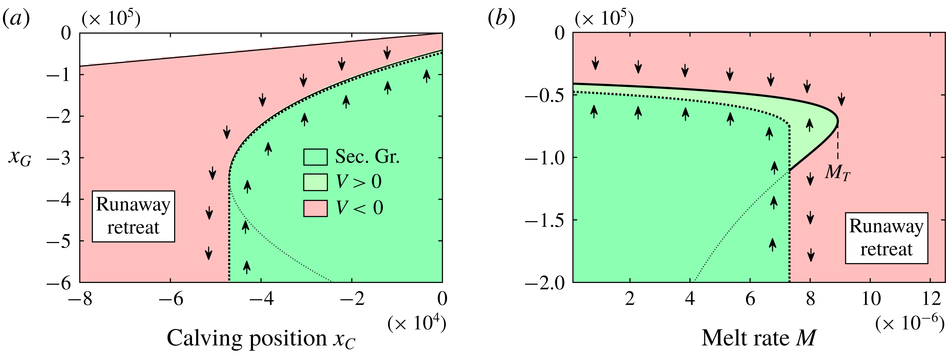
I begin in § 2 by reviewing the Q2D model and the integrated steady-state balance equation. This is followed in § 3 by the development of the primary theoretical tool referred to as the ‘stability diagram’, which is a bifurcation diagram in which steady states, their local stability and the conditions for secondary grounding are incorporated simultaneously. Section 4 applies this method to determine the stability properties of buttressed groundings and elucidates features associated with the ice-sheet structure during the recovery of a tipped grounding line. Section 5 considers the general regime diagram describing the conditions for tipping and recovery. In § 6, corresponding results incorporating power-law rheology and transitions to instability based on the retreat of the calving front and the increase in melt rate are demonstrated. I end in § 7 by summarising the key findings.
2 Model
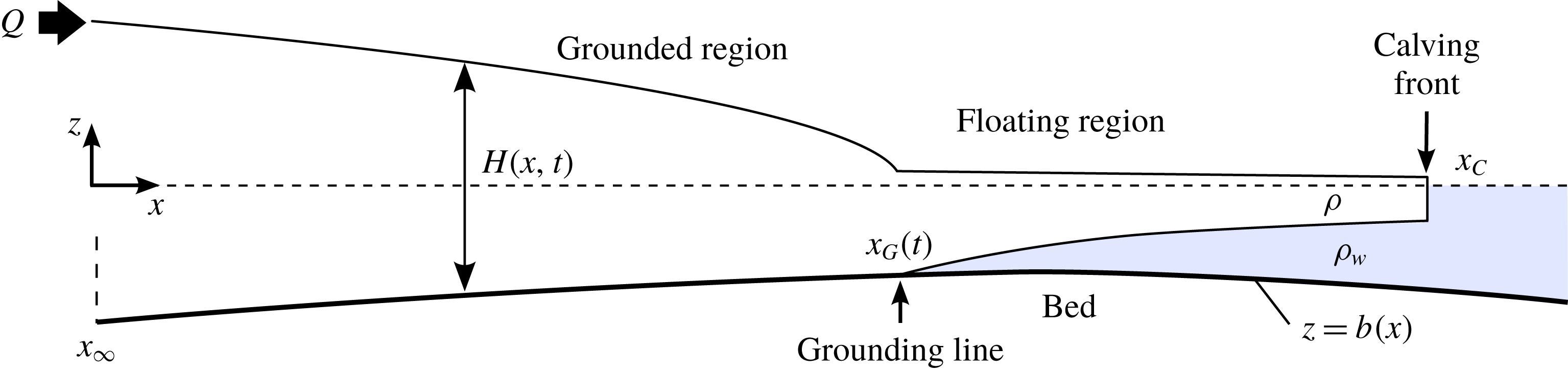
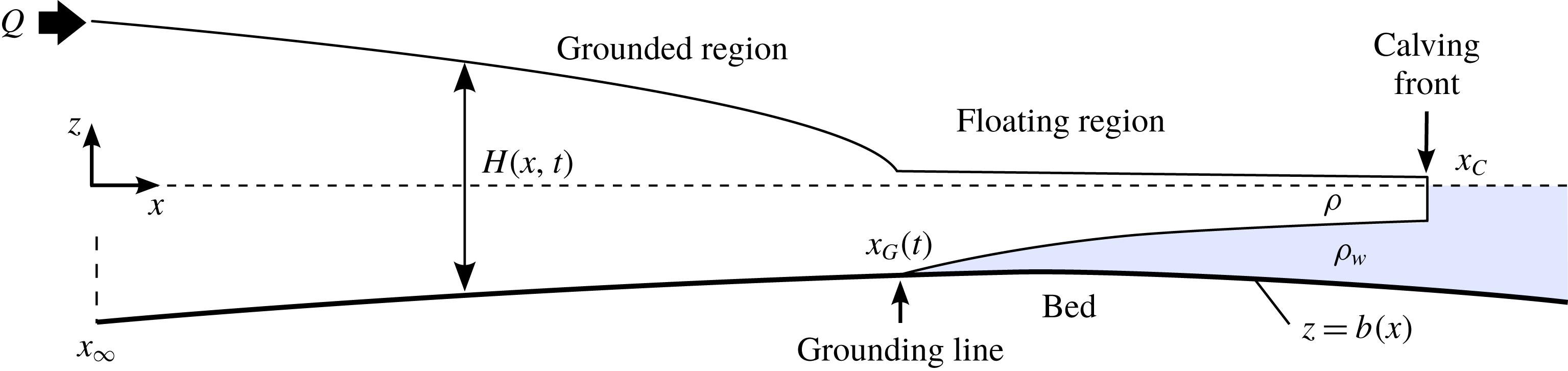
Consider a marine ice sheet comprising a viscous fluid layer (ice) of density
 $\unicode[STIX]{x1D70C}$
flowing over a rigid bed
 $z=b(x)$
and lying submerged in an effectively inviscid fluid (the ocean) of larger density
 $\unicode[STIX]{x1D70C}_{w}$
and upper surface
 $z=0$
(figure 1). The flow is subject to a no-slip condition along the margins,
 $y=\pm w(x)$
. The ice sheet generally comprises both a grounded region and a floating region – the ice shelf – which interface at the grounding line
 $x_{G}(t)$
. The grounded and floating regions can be determined at any given time by comparing the thickness profile
 $H(x,t)$
to the flotation profile
 $$\begin{eqnarray}d(x)\equiv -(\unicode[STIX]{x1D70C}_{w}/\unicode[STIX]{x1D70C})b(x),\end{eqnarray}$$
which represents the threshold thickness below which the ice sheet would float at the location
 $x$
. If
 $H(x,t)>d(x)$
, the flow is grounded at
 $x$
and if
 $H(x,t)<d(x)$
, it is floating.
Schematic of a marine ice sheet.
The flow forms an extensional thin-layer flow with differing forms of drag and gravitational forces acting on the grounded and floating components. Ice rheology is typically modelled as a shear-thinning power-law fluid, with stress proportional to the rate of deformation raised to the power
 $m=1/n$
, where
 $n$
is typically taken as 3. I model the flow using the quasi-two-dimensional (Q2D) model defined by the conditional extensional-flow equation
 $$\begin{eqnarray}\displaystyle 4\frac{\unicode[STIX]{x2202}}{\unicode[STIX]{x2202}x}\left(\unicode[STIX]{x1D707}wH\frac{\unicode[STIX]{x2202}u}{\unicode[STIX]{x2202}x}\right)=\left\{\begin{array}{@{}ll@{}}\displaystyle D(u)+\unicode[STIX]{x1D70C}gwH\left(\frac{\unicode[STIX]{x2202}H}{\unicode[STIX]{x2202}x}+\frac{\text{d}b}{\text{d}x}\right)\quad \quad & \text{if }H>d(x),\\ \displaystyle C_{+}(x)Hu^{m_{+}}+\unicode[STIX]{x1D70C}g^{\prime }wH\frac{\unicode[STIX]{x2202}H}{\unicode[STIX]{x2202}x}\quad & \text{if }H<d(x),\end{array}\right. & & \displaystyle\end{eqnarray}$$
where
 $u(x,t)$
is the width-averaged velocity,
 $\unicode[STIX]{x1D707}=\unicode[STIX]{x1D707}_{0}|\unicode[STIX]{x2202}u/\unicode[STIX]{x2202}x|^{m-1}$
is the effective viscosity,
 $\unicode[STIX]{x1D707}_{0}$
is a rheological coefficient,
 $w(x)$
is the half width of the embayment,
 $C_{+}(x)$
is the effective lateral drag coefficient,
 $D(u)$
is a function representing the total drag (lateral and basal) on the flow in the grounded region,
 $g$
is the gravitational strength, and
 $g^{\prime }\equiv (\unicode[STIX]{x1D70C}_{w}-\unicode[STIX]{x1D70C})g/\unicode[STIX]{x1D70C}_{w}$
is the reduced gravity. A benchmarking and discussion of the applicability of the Q2D model is provided in the companion paper (Pegler Reference Pegler2018). I model the total drag as the sum of the width-integrated basal and depth-integrated lateral stresses,
 $$\begin{eqnarray}D(u)=w\unicode[STIX]{x1D70F}_{b}(u)+H\unicode[STIX]{x1D70F}_{s}(u)=C_{-}(x)wu^{m_{-}}+C_{+}(x)Hu^{m_{+}},\end{eqnarray}$$
where
 $C_{-}(x)$
is the basal-drag coefficient and
 $m_{-}$
is the basal drag-law exponent. The basal stress is modelled here using a Weertman slip condition (a power-law Navier condition), which is standard in ice-sheet simulation (Cuffey & Paterson Reference Cuffey and Paterson2010). The lateral stress is instead formulated in (2.3) on the basis of a ‘shear-drag parametrisation’, which models the lateral stress heuristically as the drag stress associated with a shear-dominated transverse shear profile. For this model to be consistent with both the regime of transverse-shear-dominated flow and conservation of mass, the effective lateral drag coefficient must be taken as
 $C_{+}(x)=\unicode[STIX]{x1D707}_{0}[2^{1-n}(n+2)^{-1}w(x)]^{-(1/n)}$
with
 $m_{+}=1/n$
(Pegler Reference Pegler2016). This heuristic parametrisation of lateral shear drag yields model predictions that are, subject to the approximation of a suitably parallel flow, in good agreement with laboratory data and two-dimensional simulation of the full SSA equations across the range of wide to narrow geometries (Pegler Reference Pegler2016, Reference Pegler2018).
It should be noted that the direct summation of the two drag laws used to describe the total stress in the grounded region (2.3) is, while likely a good approximation, not necessarily accurate unless either basal or lateral stress is locally dominant. For situations where the width-integrated basal and depth-integrated lateral stresses are comparable in the grounded region, a resolution of a Poisson-type elliptic boundary-value problem could be conducted to describe a total drag on the grounded region
 $D(u)$
resulting from the mixture of basal and lateral stresses. Nonetheless, it can be anticipated that the simple addition of the two drag laws used in (2.3) may, in addition to its clear validity in the limits of either one of the contributions being much greater than the other, provide a good general approximation. This will be tested with further work.
It is worth emphasising that lateral stresses in the ice shelf and lateral stresses in the grounded region have very different roles in large-scale ice-sheet dynamics. The role of all drag stresses in the grounded region (lateral or basal) is to control the steepness of the ice sheet upstream of the grounding line, and hence the degree of ‘pile-up’ for a given grounding-line position. As discussed in Pegler (Reference Pegler2018), these stresses do not necessarily have an important control of the grounding line, which is controlled instead specifically by the resistance to flow across it. The drag stresses a short distance upstream of the grounding line play some role in influencing the extensional contribution to the resistance to flow across the grounding line, as implied by a dependence of
 $E$
on
 $D(u)$
, which will be shown in (2.10) below. For sufficiently large buttressing
 $B$
, this extensional resistance to flow across the grounding line can, however, become relatively smaller than the buttressing force even for a relatively short ice shelf. The control of the flux and position of the grounding line can then switch to being controlled almost independently by the ice shelf (Pegler Reference Pegler2018). The lateral stresses exerted in the floating region contributes directly to the resistance to flow across the grounding line and hence its position and, in turn, the stability of the entire ice sheet.
The considerably greater significance of lateral stresses in the floating region compared to lateral stresses in the grounded region can thus be understood by considering the forces against which they compete for significance. For flow in the grounded region, the competing stress is basal stress. For the flow across the grounding line, the competing stress is the extensional stress
 $E$
. Since the magnitude of the extensional stress would, in the absence of ice-shelf buttressing, provide an independent, and potentially very weak, resistance to the flow across the grounding line, it is readily possible for the lateral stresses in the floating region – despite their small magnitude compared to the basal stresses in the grounded region – to provide the dominant resistance to flow across the grounding line. In a sense, the resistance to flow across the grounding line in a marine ice sheet provides an independent ‘weak link’ in the maintenance of the large-scale ice-sheet mass balance, for which the ice-shelf buttressing provides a direct control. Consequently, ice-shelf buttressing can have a major independent control of the amount of ice that can be stored stably in the grounded region of a marine ice sheet even if generated by a relatively small ice shelf and being small in absolute magnitude compared to the basal stresses resisting the flow throughout the prevailing interior of the ice sheet.
The symmetry conditions at the ice divide
 $x_{D}$
and the stress condition at the terminus
 $x_{C}$
are given by
 $$\begin{eqnarray}\displaystyle u & = & \displaystyle 0\hphantom{\frac{rg}{1}H}\quad \text{at }x=x_{D},\end{eqnarray}$$
 $$\begin{eqnarray}\displaystyle \unicode[STIX]{x1D707}\frac{\unicode[STIX]{x2202}u}{\unicode[STIX]{x2202}x} & = & \displaystyle 0\hphantom{\frac{rg}{1}H}\quad \text{at }x=x_{D},\end{eqnarray}$$
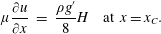 $$\begin{eqnarray}\displaystyle \unicode[STIX]{x1D707}\frac{\unicode[STIX]{x2202}u}{\unicode[STIX]{x2202}x} & = & \displaystyle \frac{\unicode[STIX]{x1D70C}g^{\prime }}{8}H\quad \text{at }x=x_{C}.\end{eqnarray}$$
While I treat
 $x_{C}$
as an imposed parameter in the examples of this paper, a more complex calving condition, e.g. on the calving thickness (Schoof et al.
Reference Schoof, Davis and Popa2017) could be incorporated into the analytical toolkit developed in this paper using an extra condition of the implicit form
 $H(x_{C})=H_{C}$
, where
 $H_{C}$
is a parameter.
Finally, the evolution equation for the thickness is
 $$\begin{eqnarray}\frac{\unicode[STIX]{x2202}H}{\unicode[STIX]{x2202}t}=-\frac{1}{w}\frac{\unicode[STIX]{x2202}}{\unicode[STIX]{x2202}x}(wHu)+f(x,t),\end{eqnarray}$$
where
 $f(x,t)$
is the net accumulation of ice.
2.1 Integrated steady-state balance equation
It will be demonstrated in this paper that the sustainment of ice-sheet stability can be understood by constructing the steady-state solutions for a given configuration of parameters. The steady states can be determined by a reduced, integrated theory (Pegler Reference Pegler2016, Reference Pegler2018), which will be reviewed as follows. In steady state, the mass conservation equation (2.7) can be integrated subject to (2.4) to yield the flux along the flow,
 $$\begin{eqnarray}q(x)=Hu=\frac{1}{w(x)}\int _{x_{D}}^{x}w(\hat{x})f(\hat{x})\,\text{d}\hat{x}.\end{eqnarray}$$
On applying this expression along with certain approximations of the components of the grounded and floating sections, expressions for the forces exerted by the steady-state profiles of the grounded and floating regions can be derived. By utilising these analytical results together, it was determined that the grounding line
 $x_{G}$
satisfies the algebraic equation
 $$\begin{eqnarray}E(x_{G})+B(x_{G})={\textstyle \frac{1}{2}}\unicode[STIX]{x1D70C}g^{\prime }d(x_{G})^{2},\end{eqnarray}$$
where the two functions on the left-hand side can be interpreted as databases that give the steady-state extensional stress and the steady-state buttressing force exerted by an ice shelf explicitly in terms of the physical parameters and grounding-line position
 $x_{G}$
. By integrating the reduced systems representing grounded and floating regions, these functions, given here in a general dimensional form, were determined as follows. The extensional resistance function is
 $$\begin{eqnarray}E(x_{G})=4\unicode[STIX]{x1D707}_{0}d(x_{G})\left[\frac{u(x_{G})}{d(x_{G})}\left(\frac{\text{d}b(x_{G})}{\text{d}x}+\frac{D[u(x_{G})]}{\unicode[STIX]{x1D70C}gw(x_{G})d(x_{G})}\right)\right]^{1/n},\end{eqnarray}$$
where
 $u(x_{G})=q(x_{G})/d(x_{G})$
. The buttressing resistance function is
 $$\begin{eqnarray}B(x_{G})=\frac{\unicode[STIX]{x1D70C}g^{\prime }}{2}\left[\left(H_{C}^{N}+\frac{N}{\unicode[STIX]{x1D70C}g^{\prime }}\int _{x_{G}}^{x_{C}}\frac{C_{+}(\hat{x})q(\hat{x})^{1/n}}{w(\hat{x})}\,\text{d}\hat{x}\right)^{2/N}-H_{C}^{2}\right],\end{eqnarray}$$
where
 $N=(n+1)/n$
, and
 $$\begin{eqnarray}H_{C}\equiv H(x_{C})=\unicode[STIX]{x1D705}\left[\left(\frac{\unicode[STIX]{x1D707}_{0}}{\unicode[STIX]{x1D70C}g^{\prime }}\right)^{n(n+1)}\left(\frac{C_{+}(x_{C})}{\unicode[STIX]{x1D707}_{0}w(x_{C})}\right)^{n}q(x_{C})^{n+1}\right]^{N^{2}}.\end{eqnarray}$$
The constant
 $\unicode[STIX]{x1D705}=3.28$
for
 $n=3$
(and
 $\unicode[STIX]{x1D705}\approx 8^{1/N^{2}}$
more generally).
The result of (2.9), with (2.10) and (2.11), forms a closed algebraic equation for steady-state grounding line positions
 $x_{G}$
, which can be solved at very minimal numerical cost. The relative saving in numerical cost compared to full numerical simulation of the SSA equations (e.g. Gudmundsson et al.
Reference Gudmundsson, Krug, Durand, Favier and Gagliardini2012) is at least ten orders of magnitude, but the numerical precision is similar for suitable geometries. The method thus provides new avenues for rapid scenario exploration and sensitivity analysis, in addition to providing physical insight into the underlying dynamics. Moreover, it does not suffer issues of spatial numerical resolution, which can be a limitation for confident grounding-line prediction. In applying these results, a number of caveats should be noted, which are summarised in Pegler (Reference Pegler2018, §8.3). These include the assumption of a suitably parallel ice-sheet flow, which, while typical of many outlets, will be limited in direct applicability to the context of narrow outlets feeding broad ice shelves, for example.
In addition to providing a useful counterpart to numerical simulation, the results of (2.9)–(2.11) provide physical insight into the parametric control of marine ice sheets. The right-hand side of (2.9) represents the driving hydrostatic pressure drop
 $(\unicode[STIX]{x1D6FF}/2)d(x)^{2}$
, a force which is purely dependent on the grounding-line thickness. The left-hand side is the sum of two distinct forces resisting this driving force: the extensional resistance,
 $E$
, and the ice-shelf buttressing force
 $B$
, which varies with respect to the calving and grounding-line positions,
 $x_{C}$
and
 $x_{G}$
. The equation (3.1) clarifies the bridge between two fundamental limiting balances. One is the unbuttressed, extension-dominated balance,
 $E(x_{G})\sim (\unicode[STIX]{x1D6FF}/2)d(x_{G})^{2}$
(this result will, subject to some further approximation, recover the unbuttressed expression for
 $Q$
given by Schoof (Reference Schoof2007b
)). In the opposite limit is the buttressing-dominated balance,
 $B(x_{G})\sim (\unicode[STIX]{x1D6FF}/2)d(x_{G})^{2}$
, which represents a distinct regime of grounding-line control referred to as ‘strong buttressing’ and arises in sufficiently narrow geometries (Pegler et al.
Reference Pegler, Kowal, Hasenclever and Worster2013). In this regime, the grounding-line dynamics does not depend on the basal conditions of the ice sheet (nor indeed any of the contributions to the mixed total drag in the grounded region (2.3)).
2.2 Example configurations and dimensionless model
While the full framework specified above is more general, for the main illustrative solutions used in this paper I will make a number of specifications designed to distil the examples to focusing specifically on the implications of lateral stresses. First, I neglect
 $\text{d}b/\text{d}x(x_{G})$
in (2.10), which I anticipate to be a good approximation for slopes of order
 $10^{-3}$
of less. I will also assume that the coefficient of basal drag
 $C_{-}$
, flow width
 $w$
and effective lateral drag coefficient
 $C_{+}$
, are uniformly constant along the flow. The basal-drag and rheological exponents will be set as equal,
 $m_{-}=m=1/n$
, and I will focus on the examples of
 $n=1$
and 3.
For my illustrative examples, I will focus on the case of a broad linear slope defined by
 $$\begin{eqnarray}b(x)=b_{0}+ax,\end{eqnarray}$$
where
 $|b_{0}|$
is the depth of the ocean at the reference position
 $x=0$
, and
 $a$
is the bed slope. Positive slopes,
 $a>0$
, correspond to a bed height that increases in the direction of flow (also termed a reverse, or retrograde slope), as is characteristic of many regions of the bedrock underlying the West Antarctic Ice Sheet at large scales. Examples of nonlinear bed slopes involving a global maximum or global minimum are provided in the supplementary document available at https://doi.org/10.1017/jfm.2018.742.
The input will be specified as being localised at the ice divide
 $$\begin{eqnarray}f(x)=2Q\unicode[STIX]{x1D6FF}(x-x_{D}),\end{eqnarray}$$
where
 $Q$
is the input flux into the region
 $x>x_{D}$
. It should be noted that the effects of a distributed net accumulation and/or loss via melting (negative
 $f(x)$
) is typical across the extent of an ice sheet. The case (2.14) nonetheless provides a useful control condition for distilling the examples to considering the effects of lateral stresses independently without the extra effect of a variable steady-state flux
 $q(x)$
. An example of a large-scale distributed accumulation
 $f(x)\neq 0$
spanning ice divide to terminus is provided by example 4 of the supplementary document. The effect of distributed melting along the underside of the ice shelf will be considered in §6 in order to demonstrate the manner in which it can trigger tipping of a grounding line.
I non-dimensionalise (2.2)–(2.7) by defining
 $$\begin{eqnarray}x\equiv {\mathcal{L}}\tilde{x},\quad t\equiv ({\mathcal{L}}/{\mathcal{U}})\tilde{t},\quad (H,b,d)\equiv {\mathcal{H}}(\tilde{H},\tilde{b},\tilde{d}),\quad u\equiv (Q/{\mathcal{H}})\tilde{u} ,\end{eqnarray}$$
where
 $$\begin{eqnarray}\displaystyle {\mathcal{H}}\equiv \left[\unicode[STIX]{x1D707}_{0}C_{-}^{m}\left(\frac{Q^{m}}{\unicode[STIX]{x1D70C}g}\right)^{m+1}\right]^{1/k_{m}},\quad {\mathcal{L}}\equiv \left[\frac{\unicode[STIX]{x1D707}_{0}^{m+2}Q^{m}}{\unicode[STIX]{x1D70C}gC_{-}^{m+1}}\right]^{1/k_{m}}, & & \displaystyle\end{eqnarray}$$
and
 $k_{m}\equiv (m+1)(m+2)-1$
. On dropping tildes, the governing equation (2.2) becomes
 $$\begin{eqnarray}\displaystyle 4\frac{\unicode[STIX]{x2202}}{\unicode[STIX]{x2202}x}\left(\unicode[STIX]{x1D707}H\frac{\unicode[STIX]{x2202}u}{\unicode[STIX]{x2202}x}\right)=\left\{\begin{array}{@{}ll@{}}\displaystyle (1+SH)u^{m}+H\left(\frac{\unicode[STIX]{x2202}H}{\unicode[STIX]{x2202}x}+\frac{\text{d}b}{\text{d}x}\right)\quad & \text{if }H>d(x),\\ \displaystyle SHu^{m}+\unicode[STIX]{x1D6FF}H\frac{\unicode[STIX]{x2202}H}{\unicode[STIX]{x2202}x}\quad & \text{if }H<d(x),\end{array}\right. & & \displaystyle\end{eqnarray}$$
where
 $\unicode[STIX]{x1D707}=|\unicode[STIX]{x2202}u/\unicode[STIX]{x2202}x|^{m-1}$
. The dimensionless input condition associated with (2.14), the symmetry condition (2.5) and the frontal stress condition (2.6) become
 $$\begin{eqnarray}\displaystyle Hu & = & \displaystyle 1\hphantom{\frac{g}{1},}\quad \text{at }x=x_{D+},\end{eqnarray}$$
 $$\begin{eqnarray}\displaystyle \unicode[STIX]{x1D707}\frac{\unicode[STIX]{x2202}u}{\unicode[STIX]{x2202}x} & = & \displaystyle 0\hphantom{\frac{g}{1},}\quad \text{at }x=x_{D},\end{eqnarray}$$
 $$\begin{eqnarray}\displaystyle \unicode[STIX]{x1D707}\frac{\unicode[STIX]{x2202}u}{\unicode[STIX]{x2202}x} & = & \displaystyle \frac{\unicode[STIX]{x1D6FF}}{8}H\quad \text{at }x=x_{C},\end{eqnarray}$$
where the plus subscript is used to define a limit from the positive
 $x$
direction. The evolution equation (2.7) becomes
 $$\begin{eqnarray}\displaystyle \frac{\unicode[STIX]{x2202}H}{\unicode[STIX]{x2202}t}=-\frac{\unicode[STIX]{x2202}}{\unicode[STIX]{x2202}x}(Hu). & & \displaystyle\end{eqnarray}$$
In addition to the positions
 $x_{D}$
and
 $x_{C}$
, the dimensionless model depends on two dimensionless parameters:
 $$\begin{eqnarray}\displaystyle S\equiv \frac{{\mathcal{H}}C_{+}}{wC_{-}},\quad \unicode[STIX]{x1D6FF}\equiv \frac{g^{\prime }}{g}, & & \displaystyle\end{eqnarray}$$
representing the dimensionless lateral shear-drag coefficient and the density difference, respectively. As estimated in Pegler (Reference Pegler2018),
 $S=0$
–
 $10^{-2}$
, with
 $S=0$
recovering the case of a one-dimensional marine ice sheet. The value
 $\unicode[STIX]{x1D6FF}=0.1$
will be assumed throughout my analysis. The value
 $x_{D}=-3\times 10^{3}$
will be used for my illustrative time-dependent numerical solutions. Finally, the dimensionless form of the linear bed height (2.13) is
 $$\begin{eqnarray}\displaystyle b(x)=-\unicode[STIX]{x1D6FD}+\unicode[STIX]{x1D6FC}x,\quad \text{where }\unicode[STIX]{x1D6FC}\equiv ({\mathcal{L}}/{\mathcal{H}})a,\quad \unicode[STIX]{x1D6FD}\equiv |b_{0}|/{\mathcal{H}}, & & \displaystyle\end{eqnarray}$$
are a scaled bed slope and reference ocean depth, respectively.
3 Construction of a grounding-line stability diagram
This section develops the analytical methodology used to visualise the determinants of global stability of a marine ice sheet for a given configuration. A method is developed based on the construction of effective stability (bifurcation) diagrams for grounding lines that unify steady states, the natures of their local stability (attractor versus repeller) and the inducement of secondary grounding within a single parameter–stability diagram.
3.1 Steady states
The first component of the methodology is provided by the steady-state equation (2.9). In dimensionless form, along with the simplifications described in §2.2, this equation reads
 $$\begin{eqnarray}E[d(x_{G})]+B(x_{G},x_{C})={\textstyle \frac{1}{2}}\unicode[STIX]{x1D6FF}d(x_{G})^{2}.\end{eqnarray}$$
For linear rheology,
 $n=1$
, the reduced forms of the resistance functions (2.10) and (2.11) are given by
 $$\begin{eqnarray}\displaystyle E[d(x_{G})]\approx 4d(x_{G})^{-3},\quad B(x_{G},x_{C})=-S(x_{C}-x_{G}). & & \displaystyle\end{eqnarray}$$
For simplicity, I have here also neglected a contribution to
 $E$
owing to the lateral stresses in the grounded region, represented by the second term in (2.3). This contribution may have some slight effect on the grounding line. As noted above, the lateral stresses in the floating region are, despite their similar absolute magnitude, fundamentally more important to global ice-sheet stability because of their direct resistance to flow across a grounding line (Pegler Reference Pegler2018).
3.2 Local stability
A steady-state grounding-line position, as predicted by (3.1) and (3.2), will either be an attractor (stable) or a repeller (unstable). In the context of unbuttressed grounding-line dynamics, a negatively sloped bedrock,
 $b^{\prime }(x_{G})<0$
, generally results in an attractor while a positively sloped bedrock results in a repeller (at least subject to the simplification of a uniform drag coefficient which, as highlighted at the end of this subsection, can affect stability along with any other spatial parametric variation that determines
 $E(x)$
). These basic stability results arise because an unbuttressed grounding line perturbed backwards from a steady state on a positive bed slope will increase the grounding-line thickness and hence the driving buoyancy force, thereby stimulating further retreat, i.e. a positive-feedback response to the original perturbation. Conversely, perturbation of an unbuttressed grounding line on a negative slope produces negative feedback and attraction back to the original steady state. This has been argued previously on the basis of the relationship between grounding-line flux and thickness applicable to an unbuttressed grounding line and linear stability analyses (Schoof Reference Schoof2007a
; Wilchinsky Reference Wilchinsky2009; Fowler Reference Fowler2011; Schoof Reference Schoof2012). These properties of local stability do not apply to the buttressed case.
In order to assess the stability of a general grounding line, I propose a method based on evaluating the function
 $$\begin{eqnarray}V(x)=E[d(x)]+B(x,x_{C})-{\textstyle \frac{1}{2}}\unicode[STIX]{x1D6FF}d(x)^{2},\end{eqnarray}$$
which represents the ‘imbalance’ associated with the steady-state forces in (3.1). If
 $V(x_{G})=0$
, there is a steady state at
 $x_{G}$
. The gradient
 $V^{\prime }(x_{G})$
will indicate the nature of stability of the steady state at
 $x_{G}$
directly in the manner of an autonomous evolution rule, ‘
 ${\dot{x}}\propto V(x_{G})$
’. To explain this, note first that the function
 $V(x_{G})$
will indicate stability correctly in this way for the unbuttressed case, as I verify directly below. Its general functioning then follows from the fact that the nature of an isolated steady-state branch across a bifurcation diagram is conserved under continuous parametric variation. A more rigorous proof of the functioning of
 $V$
is beyond the scope of this paper but, to gain confidence in its functioning, I include a supplementary document with a suite of examples validated using time-dependent integrations, in addition to those provided later in the paper (figures 5 and 9).
Because (3.3) depends purely on known analytic expressions, it affords a versatile direct assessment of steady states and their local stability that, as far as the qualitative question of local stability is concerned, bypasses the need for any linear stability analysis or consideration of a flux relationship. The method applies for generalised physical situations described by the functions of (2.10) and (2.11) (with or without buttressing). Since any determinant of the spatial variation of
 $E$
and
 $B$
will change
 $V$
, it follows that the spatial variation in
 $x$
of any one of the physical parameters, including rheological variation,
 $\unicode[STIX]{x1D707}(x)$
, the net accumulation/melt distributions of the ice sheet and ice shelf,
 $f(x)$
, the calving law, spatial variations in the coefficients of basal and lateral drag,
 $C_{-}(x)$
and
 $C_{+}(x)$
, the flow width
 $w(x)$
, and the local slope
 $b^{\prime }(x)$
, will all affect local stability. It is worth remarking that, as highlighted at the beginning of this subsection, spatial variation in the coefficient of basal drag or indeed any of the other parameters controlling
 $E$
as defined by (2.10) could, in principle, allow for stability of a grounding line on a retrograde slope even in the unbuttressed case. An unbuttressed grounding line can therefore form stably on a retrograde slope for suitable spatial variations of the determinants of
 $E$
.
In order to verify that
 $V^{\prime }$
correctly indicates the nature of stability in the unbuttressed case,
 $B=0$
, note that, in this case, (3.3) simplifies to
 $$\begin{eqnarray}V(x)=E[d(x)]-{\textstyle \frac{1}{2}}\unicode[STIX]{x1D6FF}d(x)^{2}\equiv V_{U}[d(x)].\end{eqnarray}$$
Uniquely in the unbuttressed case,
 $V$
is thus a pure function of the flotation thickness
 $d(x)$
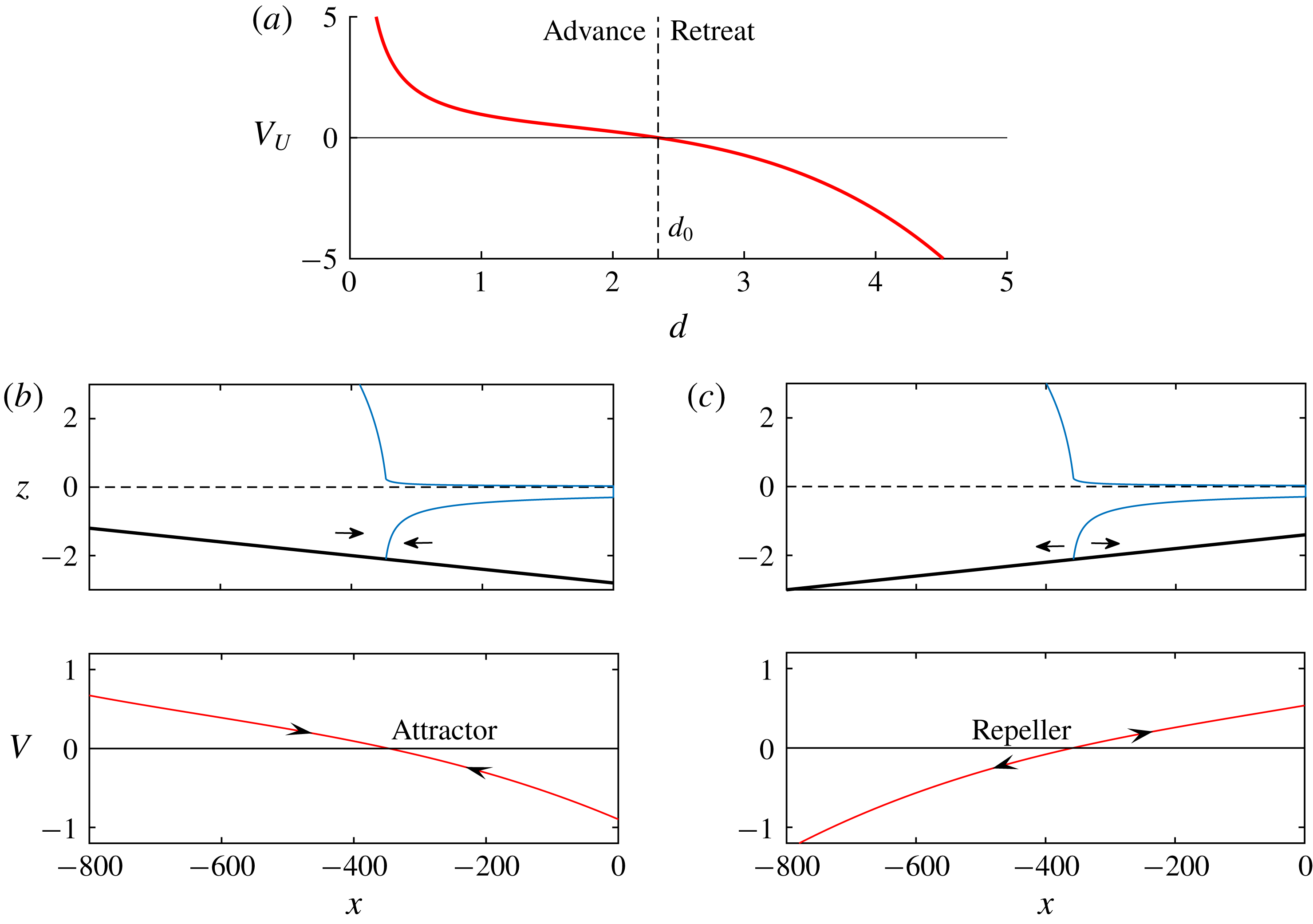
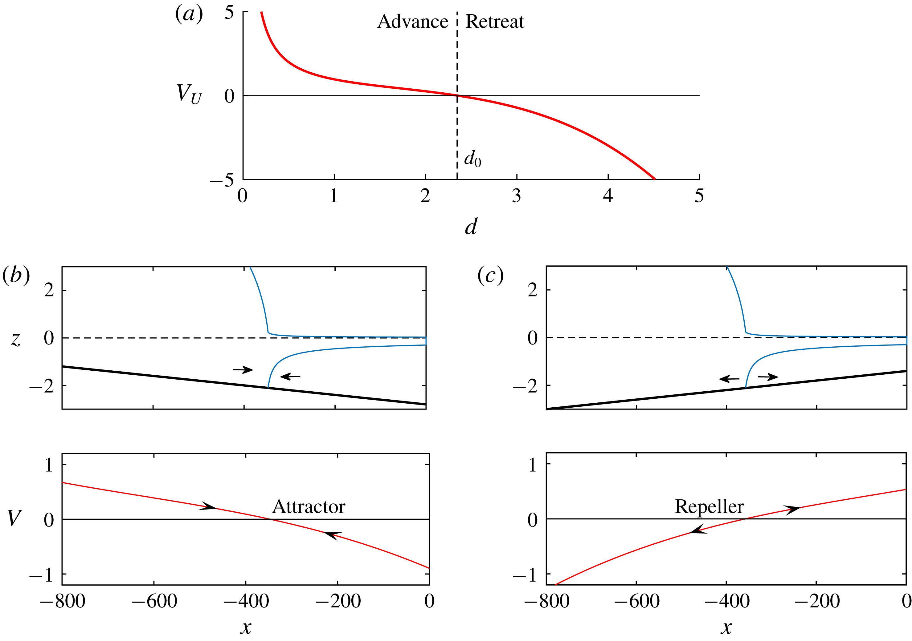
. The plot of
 $V_{U}(d)$
, given in figure 2(a) for
 $n=1$
, shows that a steady state occurs wherever the grounding-line thickness equals
 $d=d_{0}\approx 2.345$
. The plot illustrates that
 $V_{U}^{\prime }(d)<0$
. Thus, on combining this result with the chain rule
 $V^{\prime }(x)=d^{\prime }(x)V_{U}^{\prime }(d)$
, it follows that
 $\operatorname{sgn}[V^{\prime }(x)]=\operatorname{sgn}[b^{\prime }(x)]$
, confirming that the steady state is stable if
 $b^{\prime }(x_{G})<0$
and unstable if
 $b^{\prime }(x_{G})>0$
. The value of
 $V(x)$
evaluated for examples of a negative and a positive bed slope are shown in figures 2(b,c), confirming a stable and unstable state, respectively, in agreement with the time-dependent examples given in Pegler (Reference Pegler2018, figure 3(a,c)).
The relationship between the stability variable
 $V(x)=V_{U}[d(x)]$
and the grounding-line thickness
 $d$
for an unbuttressed grounding line (3.4). In this simplified situation, retreat occurs if the grounding-line thickness
 $d$
is larger than the critical value
 $d_{0}$
, and advance occurs if it is less than
 $d_{0}$
, where
 $d_{0}\approx 2.345$
is the universal dimensionless thickness at which any unbuttressed steady-state grounding line occurs,
 $V_{U}(d_{0})=0$
. Panels (b) and (c) show the stability variable
 $V(x)$
predicted by (3.3) for cases of (a) a negative bed slope
 $\unicode[STIX]{x1D6FC}=-2\times 10^{-3}$
and
 $\unicode[STIX]{x1D6FD}=2.8$
, and (b) the positive bed slope
 $\unicode[STIX]{x1D6FC}=2\times 10^{-3}$
and
 $\unicode[STIX]{x1D6FD}=1.4$
, each with zero buttressing, illustrating a local attractor and repeller, respectively. The arrows in the insets show the direction of grounding-line migration following perturbation from the steady state, as implied by the sign of
 $V(x)$
.
In addition to providing a clear visualisation of the direction of migration of a perturbed grounding line, the function
 $V(x)$
given by (3.3) provides physical insight into the general control of local stability. If a term comprising
 $V$
decreases with
 $x$
then the effect it represents contributes towards local stabilisation, and vice versa. For example, buoyancy,
 $-(\unicode[STIX]{x1D6FF}/2)d(x)^{2}$
, creates a stabilising, negative-feedback effect if
 $b^{\prime }<0$
and a positive-feedback effect if
 $b^{\prime }>0$
. The extensional resistance
 $E[d(x)]=4d^{-3}$
given by (3.2a
) is, like buoyancy, also a decreasing function of
 $d$
and will therefore have a qualitatively similar effect on promoting negative or positive feedback as the buoyancy force. However, it should be noted that for
 $n=3$
,
 $E[d(x)]=4d(x)^{-0.25}$
is only very weakly dependent on
 $x$
and thus has practically no effect on the control of local stability. The buttressing force
 $B(x_{G},x_{C})$
, given by (2.11) or (3.2b
), is, in contrast to the functions representing the buoyancy force and extensional stress, always a decreasing function of the grounding-line position
 $x_{G}$
(a longer ice shelf generates more buttressing), and thus has an unconditionally stabilising effect (this is true at least for the case of a prescribed
 $x_{C}$
assumed here; this relationship is not necessarily as straightforward for cases where
 $x_{C}$
is controlled implicitly by a condition based on a critical thickness,
 $H=H_{C}$
(Schoof et al.
Reference Schoof, Davis and Popa2017)). If
 $b^{\prime }(x)<0$
, buttressing will reinforce the negative-feedback effect of buoyancy on a negative slope. For a positive slope,
 $b^{\prime }(x_{G})>0$
, buttressing and buoyancy act in opposition: retreat of the grounding line will increase both buoyancy and buttressing. Thus, if the increase in buttressing following a retreat of a grounding line exceeds the increase in buoyancy critically, then the positive-feedback response, which would occur in the absence of buttressing, will be suppressed.
3.3 Secondary grounding
The final step of constructing the stability diagram is to determine the grounding-line positions
 $x$
for which the steady-state profile of the ice shelf produced would experience secondary grounding. As described in Pegler (Reference Pegler2018, §6), there are two kinds of secondary grounding. Either the ice shelf is predicted to penetrate the bedrock immediately at the grounding line (type I) or further downstream (type II). The critical boundary of the region of a parameter space in which secondary grounding occurs is given by the critical satisfaction of the cotangency conditions between the ice shelf and the bedrock at the grounding line,
 $$\begin{eqnarray}\displaystyle H(x_{G})=d(x_{G}),\quad H^{\prime }(x_{G})=d^{\prime }(x_{G}). & & \displaystyle\end{eqnarray}$$
This condition represents both the critical transition between no secondary grounding and type I, as well as the transition between type I and type II. My numerical approach for determining these transitions is detailed in Pegler (Reference Pegler2018), along with the more straightforward analytical approach available for
 $n=1$
.
For grounding-line positions invalidated by secondary grounding, the stability variable (3.3) fails to apply because the expression for the buttressing force (3.2b ) is based on an assumption of continuous flotation between the grounding line and the calving front. It will be demonstrated later that the critical occurrence of secondary grounding leads to a surprising effect of unconditionally reversing tipped grounding-line retreat, with the direction of grounding-line migration indicated by (3.3) being directly overridden.
4 The critical transitions to and from marine ice sheet instability
Lateral stresses impact ice-sheet stability in three fundamentally distinct ways. One is to introduce the buttressing force
 $B(x_{G},x_{C})$
directly into the balance equation (3.1). The second is to induce secondary grounding by thickening the ice shelf. A third is the contribution to the total drag in the grounded region (2.3). This section will focus on demonstrating the potential for the first two of these effects to provide the leading-order control of the onset and reversal of tipped grounding-line retreat (marine ice sheet instability). The analysis is divided into three subsections – one addressing a negative bed slope, and two addressing a positive slope – which account for all the qualitatively different regimes of stabilisation that are possible for a broad line slope.
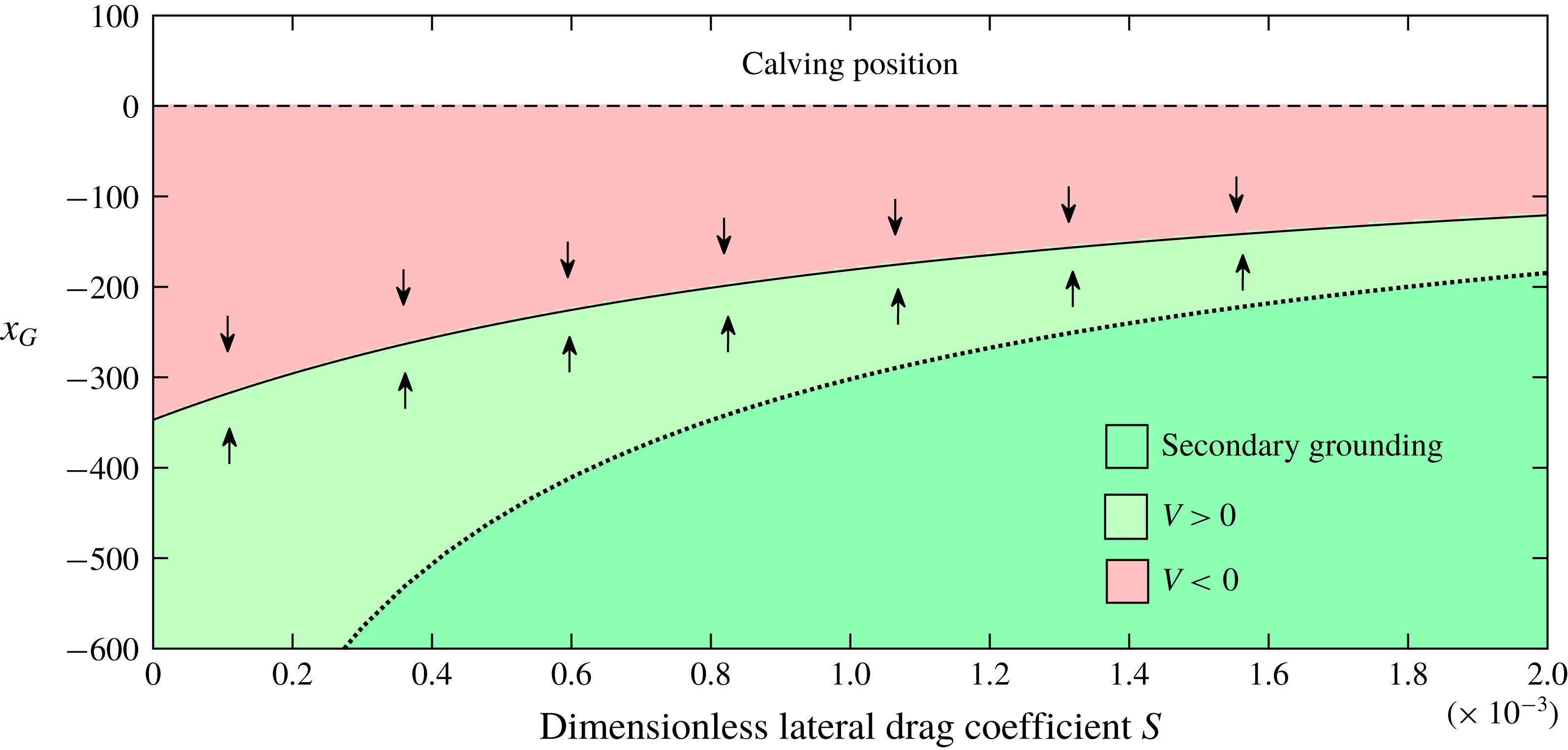
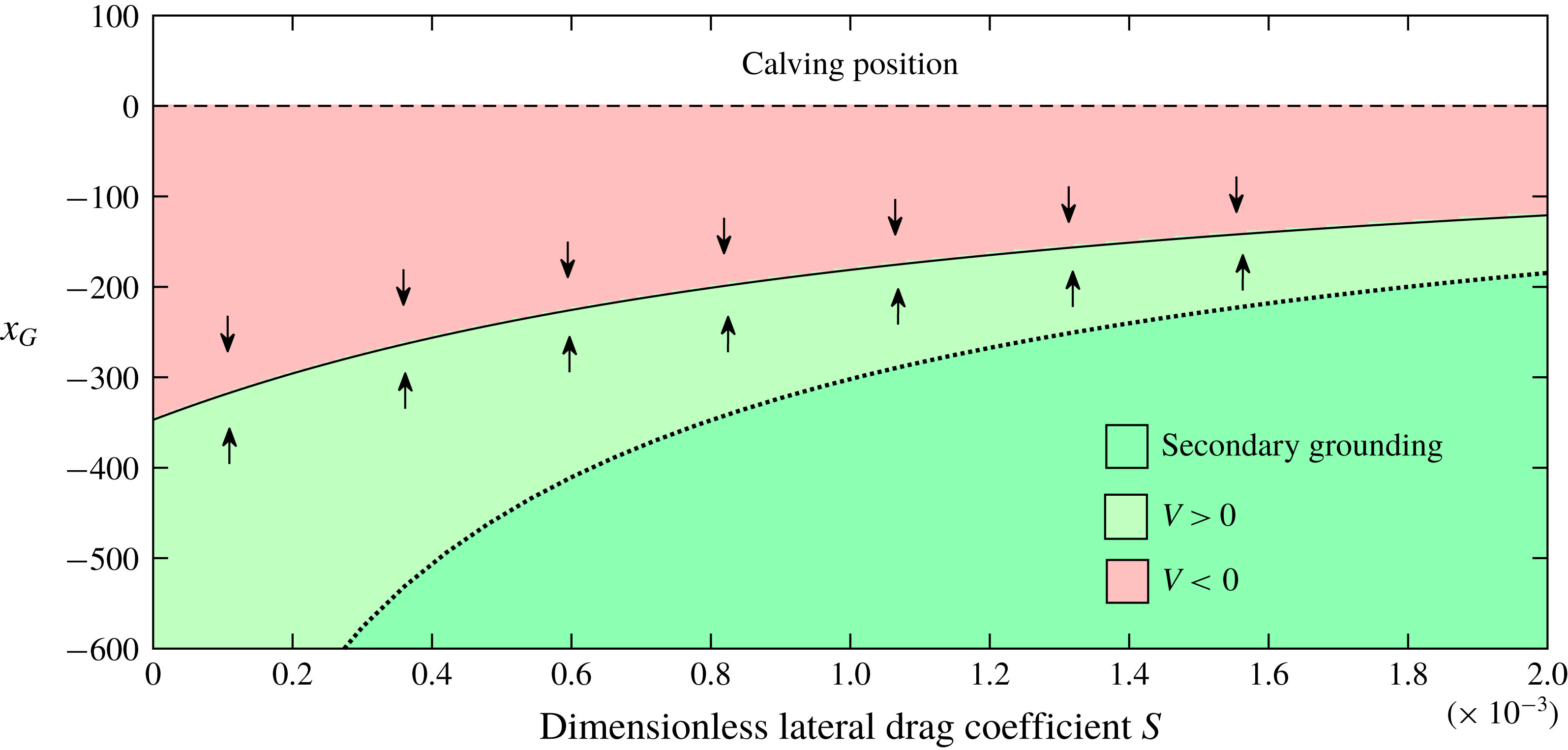
The stability diagram for the negative slope
 $\unicode[STIX]{x1D6FC}=-2\times 10^{-3}$
, reference ocean depth
 $\unicode[STIX]{x1D6FD}=2.8$
and calving position
 $x_{C}=0$
, shown as a continuous variation of the dimensionless lateral shear-drag coefficient
 $S$
, illustrating its variation from the unbuttressed case
 $S=0$
to buttressed cases
 $S>0$
. The colour scale indicates the sign of the stability variable
 $V(x)$
evaluated using (3.3). Green represents grounding-line advancement (
 $V>0$
) and red represents retreat (
 $V<0$
). The solution to the steady-state equation (3.1) is shown as a solid curve. The dark green region with a dotted outline represents grounding-line positions for which the steady-state ice shelf produces secondary grounding. The portrait illustrates the existence of a stable steady state for all values of
 $S$
.
4.1 A negative bed slope
For a negative bed slope,
 $\unicode[STIX]{x1D6FC}<0$
, buoyancy has a stabilising effect that is reinforced by ice-shelf buttressing. To illustrate this, I construct the stability diagram for the example of
 $\unicode[STIX]{x1D6FC}=-2\times 10^{-3}$
,
 $\unicode[STIX]{x1D6FD}=2.8$
and
 $x_{C}=0$
, as a continuous variation against the drag parameter
 $S$
, showing its variation from the unbuttressed case
 $S=0$
to the buttressed cases
 $S>0$
. The result is shown in figure 3, where the colour indicates the sign of the stability variable
 $V(x)$
evaluated using (3.3): red represents retreat (
 $V<0$
), green represents advance (
 $V>0$
). The steady-state solution to (3.1) is shown as a solid curve. The region of the space for which the steady-state ice shelf produces secondary grounding is shown coloured darker with a dotted outline. The plot confirms that a stable steady state arises for all values of
 $S$
. The exclusive effect of lateral stresses is to cause the steady state to lie further downstream.
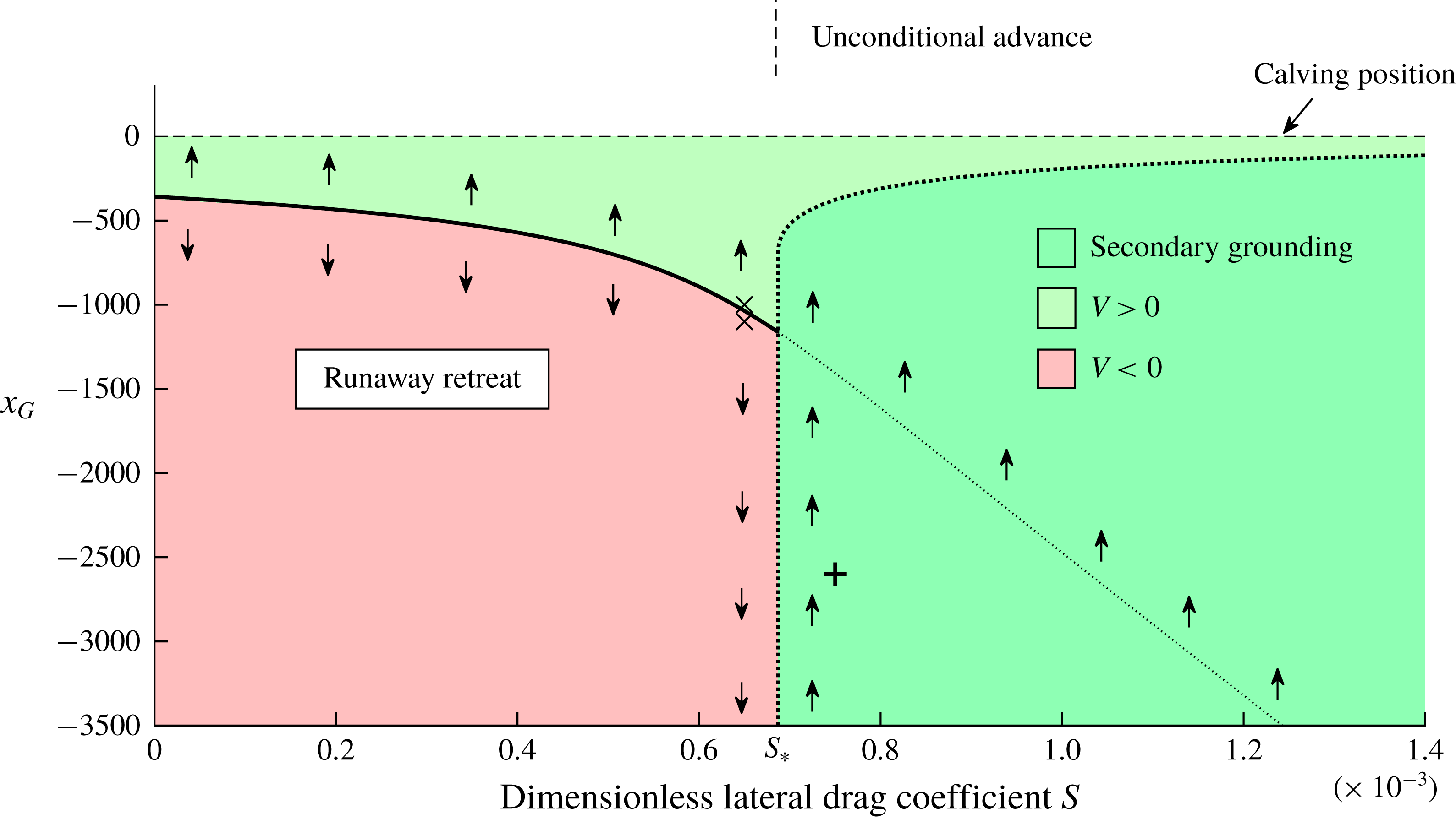
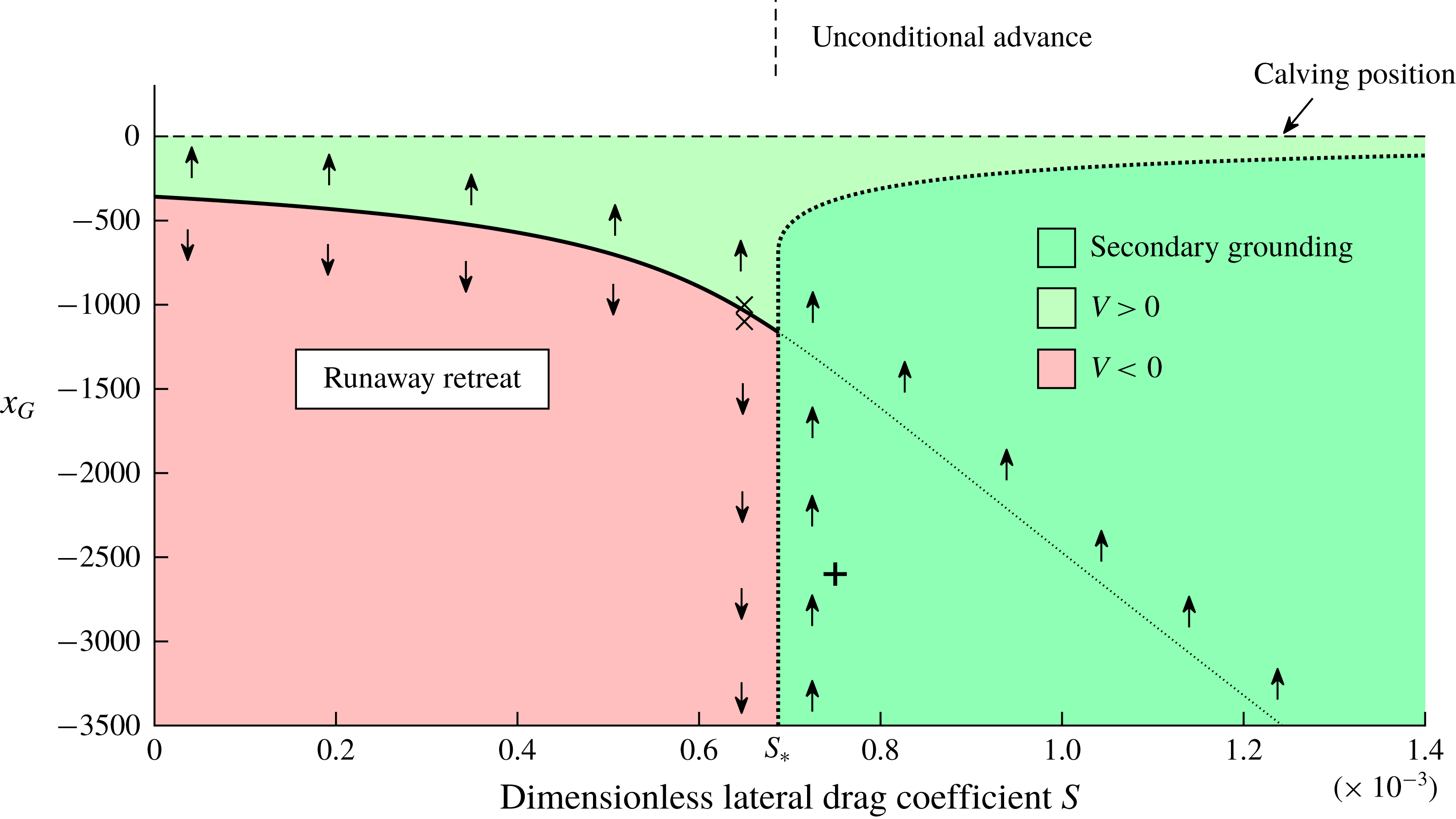
The stability diagram for the positive bed slope
 $\unicode[STIX]{x1D6FC}=2\times 10^{-3}$
, reference ocean depth
 $\unicode[STIX]{x1D6FD}=1.4<\unicode[STIX]{x1D6FD}_{0}$
and calving position
 $x_{C}=0$
, shown as a continuous variation of
 $S$
. The colour scale indicates the sign of the stability variable
 $V(x)$
evaluated using (3.3). Green represents grounding-line advancement (
 $V>0$
) and red represents retreat (
 $V<0$
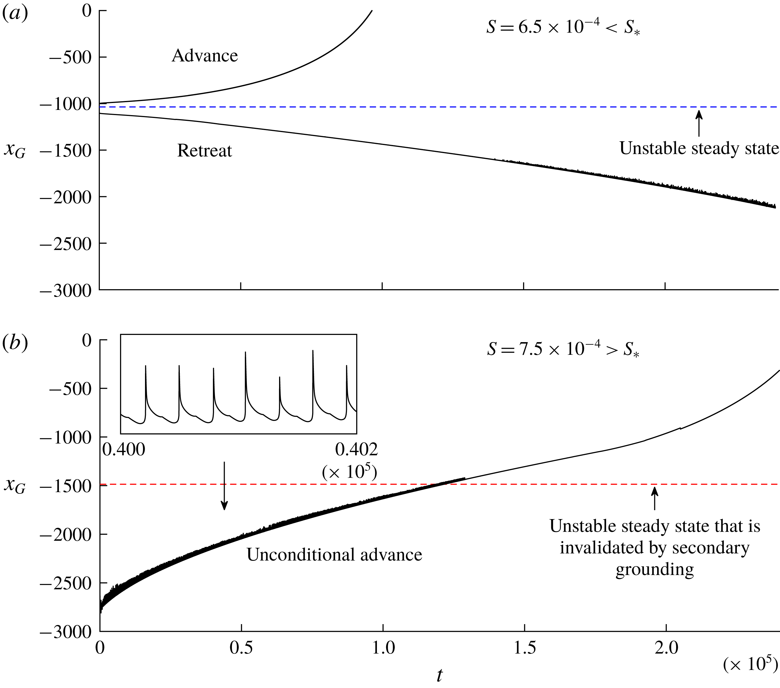
). The dark green region with a dotted outline represents the region in which secondary grounding is predicted to occur in steady state. As confirmed by the numerical result of figure 5(b), the instance of secondary grounding overrides the direction of stability indicated by (3.3), with the result of producing unconditional grounding-line advancement. The solution to (3.1) is shown as a solid curve, and as a dotted curve in the region of secondary grounding. For values of
 $S<S_{\ast }(\unicode[STIX]{x1D6FC},\unicode[STIX]{x1D6FD})\approx 6.9\times 10^{-4}$
, there is a single unstable steady state. Above the critical value,
 $S>S_{\ast }(\unicode[STIX]{x1D6FC},\unicode[STIX]{x1D6FD})$
, secondary grounding invalidates the steady state and completely suppresses the possibility of runaway retreat, in correspondence with the numerical results of figure 5(b) below. The initial grounding-line positions for the solutions of figure 5(a) are shown as crosses. That of figure 5(b) is shown as a plus sign.
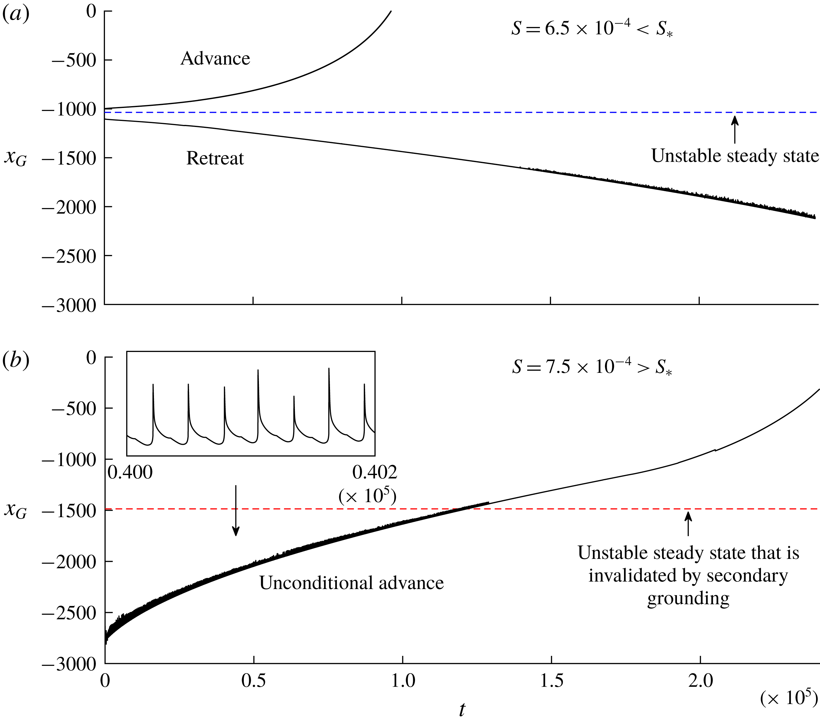
Grounding-line evolutions
 $x_{G}(t)$
predicted by the numerical solution to (2.17)–(2.21) for the positive bed slope
 $\unicode[STIX]{x1D6FC}=2\times 10^{-3}$
, reference ocean depth
 $\unicode[STIX]{x1D6FD}=1.4$
, ice-divide position
 $x_{D}=-3000$
, and (a) a subcritical drag parameter
 $S=6.5\times 10^{-4}<S_{\ast }$
and (b) the slightly larger, supercritical value
 $S=7.5\times 10^{-4}>S_{\ast }$
. The evolutions in (a) illustrate advance and retreat either side of the unstable steady state, confirming the direction of migration predicted by the stability variable (3.3). For (b), the grounding line is initialised deeply into the region where the stability variable (3.3) predicts retreat,
 $V<0$
. Nevertheless, a net advance of the grounding line occurs as a consequence the additional buttressing generated by basal stresses in a ‘marginal-flotation zone’ in front of the grounding line. The intermittent ‘grazing’ between the ice shelf and the bedrock in this region produces an oscillation in
 $x_{G}(t)$
, which is illustrated by the enlargement in the inset of (b).
It should be noted that the region in which secondary grounding is predicted only overlays the region in which
 $V>0$
. Since secondary grounding can only increase the buttressing force at the primary grounding line, any secondary grounding will simply reinforce the prediction of the stability variable (3.3) that the grounding line advances. Therefore, the dark green region can, in this case, assuredly produce grounding-line advancement; a grounding line initiated in the dark green region will advance into the lighter green region and on to the steady state.
4.2 A positive bed slope
For a positive bed slope,
 $\unicode[STIX]{x1D6FC}>0$
, the stabilising effect of ice-shelf buttressing instead competes against buoyancy, creating richer dynamics. Recall from above that any unbuttressed steady-state grounding line (
 $S=0$
) for
 $\unicode[STIX]{x1D6FC}>0$
is locally unstable and occurs at the critical thickness
 $d_{0}$
, i.e. at the dimensionless ocean depth
 $$\begin{eqnarray}\unicode[STIX]{x1D6FD}_{0}=d_{0}(1-\unicode[STIX]{x1D6FF})\approx 2.11.\end{eqnarray}$$
If
 $\unicode[STIX]{x1D6FD}<\unicode[STIX]{x1D6FD}_{0}$
, an unstable steady state for
 $S=0$
therefore occurs at the position
 $x_{G}=(\unicode[STIX]{x1D6FD}-\unicode[STIX]{x1D6FD}_{0})/\unicode[STIX]{x1D6FC}$
. If instead
 $\unicode[STIX]{x1D6FD}>\unicode[STIX]{x1D6FD}_{0}$
, no such steady state exists and, in accordance with the prediction of (3.4) that
 $V<0$
if
 $|b|>\unicode[STIX]{x1D6FD}_{0}$
, an unbuttressed grounding line would retreat unconditionally. Thus, the form of the stability diagram differs qualitatively depending on whether
 $\unicode[STIX]{x1D6FD}$
is greater than or less than
 $\unicode[STIX]{x1D6FD}_{0}$
.
4.2.1 The case
 $\unicode[STIX]{x1D6FD}/\unicode[STIX]{x1D6FD}_{0}<1$

Beginning with the case
 $\unicode[STIX]{x1D6FD}/\unicode[STIX]{x1D6FD}_{0}<1$
, I show the continuous variation of the stability diagram with
 $S$
constructed for
 $\unicode[STIX]{x1D6FC}=2\times 10^{-3}$
,
 $\unicode[STIX]{x1D6FD}=1.4<\unicode[STIX]{x1D6FD}_{0}$
and
 $x_{C}=0$
in figure 4. The initial effect of introducing lateral stresses is to cause the unstable steady state to move upstream. This produces a more secure ice-sheet configuration because a grounding line must be displaced further upstream in order for runaway retreat to trigger. The hysteresis effect discussed previously in the unbuttressed context (Schoof Reference Schoof2007a
) can therefore apply to a buttressed grounding line. However, the grounding line must be displaced further upstream in order for positive-feedback retreat to instigate following a restoration of parameters. At the critical drag parameter
 $S_{\ast }\approx 6.9\times 10^{-4}$
, secondary grounding abruptly invalidates the consistency of the unstable steady state predicted by (3.1). The region in which secondary grounding is predicted in steady state is shown as a dark green region outlined by a thick dotted curve. The invalidated steady-state solution to (3.1) is shown as a thin dotted curve extended into this region. For
 $S<S_{\ast }$
, collapse of the ice sheet occurs conditionally on the grounding-line position lying upstream of the unstable steady state (similarly to the unbuttressed case,
 $S=0$
). For
 $S>S_{\ast }$
, the question of grounding-line migration is complicated fundamentally by the potential interference of secondary grounding. For the case of negative bed slope considered above, the qualitative effect of secondary grounding on the direction of grounding-line migration was not a point of uncertainty because secondary grounding simply reinforces the prediction of advance already indicated by the stability variable,
 $V>0$
. In the present case, secondary grounding instead covers a considerable region for which the stability variable predicts retreat (
 $V<0$
) and it is therefore possible – in principle – for secondary grounding to suppress the grounding-line retreat that would occur in this situation if the ice shelf was to remain fully floating.
To investigate the possible interference of secondary grounding, I conducted time-dependent numerical calculations of the full equations (2.17)–(2.21) for values of
 $S$
which straddle the two side of the critical threshold
 $S_{\ast }$
. The Lagrangian numerical scheme applied is detailed in Pegler (Reference Pegler2018). The computations were initialised using fully developed grounded and floating regions represented by the uniform-flux solutions to (2.17). The ice-divide position is chosen as
 $x_{D}=-3\times 10^{3}$
. For
 $S>S_{\ast }$
, the secondary grounding implies that the steady-state ice shelf produced at this position would intersect the bedrock; for these cases, I initialised the shelf using the steady-state profile (derived in Pegler (Reference Pegler2016) and reviewed by Pegler (Reference Pegler2018, (5.1))) clipped along the bedrock, leaving a shallow gap initially between the base of the ice shelf and the bedrock.
As a benchmark, I first consider the marginally subcritical value of
 $S=6.5\times 10^{-4}<S_{\ast }$
, for which secondary grounding is not predicted in steady state, and corroborate the direction of grounding-line migration predicted by the sign of the stability variable (3.3). The evolutions of a grounding line initiated just upstream and just downstream of the unstable state are shown in figure 5(a). These initial positions are indicated by crosses in figure 4. The evolutions confirm the onset of a continuous advance or retreat, thus verifying the direction of grounding-line migration predicted by the sign of
 $V$
. The results show that a buttressed grounding line will undergo runaway tipped retreat if the buttressing is insufficient to outweigh the destabilising effect of buoyancy. An apparent oscillation in
 $x_{G}(t)$
for the retreating example represents some periodic secondary contacts between the ice shelf and the bedrock. Despite these contacts, collapse of the ice sheet ultimately occurs.
Next, I consider the marginally supercritical value
 $S=7.5\times 10^{-4}>S_{\ast }$
. The grounding-line evolution for this example is shown in figure 5(b). Here, I initiated the grounding line far upstream into the (dark green) region where retreat is predicted in the absence of secondary grounding,
 $V<0$
, at
 $x_{G}(0)=-2.6\times 10^{3}$
(shown as a plus sign in figure 4). In direct contradiction to the sign of
 $V$
, the grounding line undergoes a persistent net advancement. This conclusion stands in remarkable contrast to the runaway retreat occurring for the slightly smaller, marginally subcritical value
 $S=6.5\times 10^{-4}$
shown in figure 5(a). The retreat is suppressed by added buttressing generated by intermittent contacts between the ice shelf and the bedrock; the periodic surges in the buttressing force generated by the contacts produces the oscillation in
 $x_{G}(t)$
shown in the inset of figure 5(b). The prediction of secondary grounding in steady state therefore overrides the prediction of grounding-line retreat indicated by the sign of the stability variable (3.3), with the result of unconditional advance. The buttressing arising from lateral stresses alone, as predicted by (3.2b
) and assumed in evaluating (3.3), considerably underestimates the effective buttressing force generated over time as a consequence of intermittent grounding of localised sections of the ices shelf over an extended region in front of the grounding line. The criterion for secondary grounding,
 $S>S_{\ast }(\unicode[STIX]{x1D6FC},\unicode[STIX]{x1D6FD})$
, creates a sharp threshold separating conditions producing runaway grounding-line retreat from those resulting in unconditional advance. The hysteresis effect possible for
 $S<S_{\ast }$
is thereby eliminated, leading to complete suppression of grounding-line retreat.
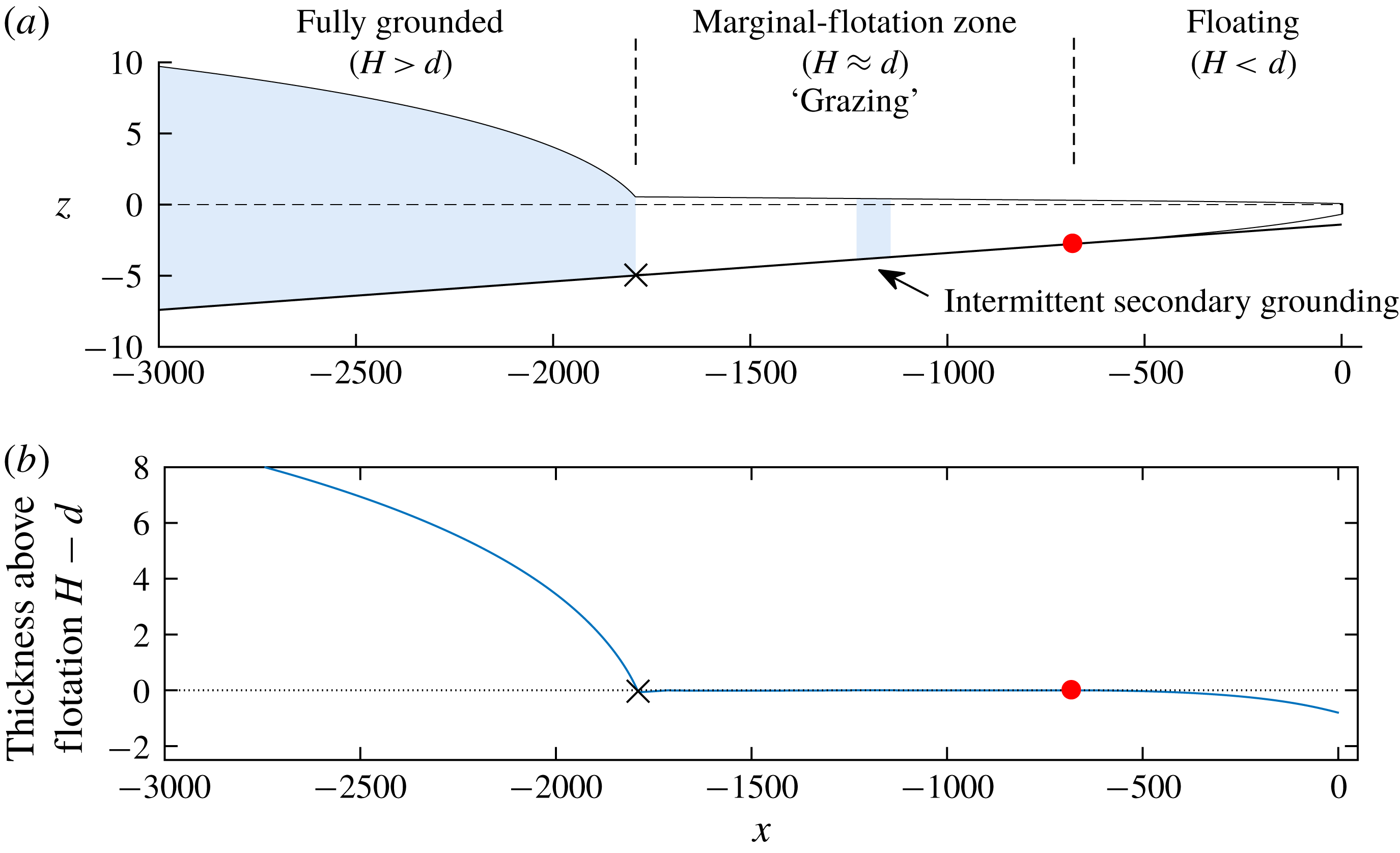
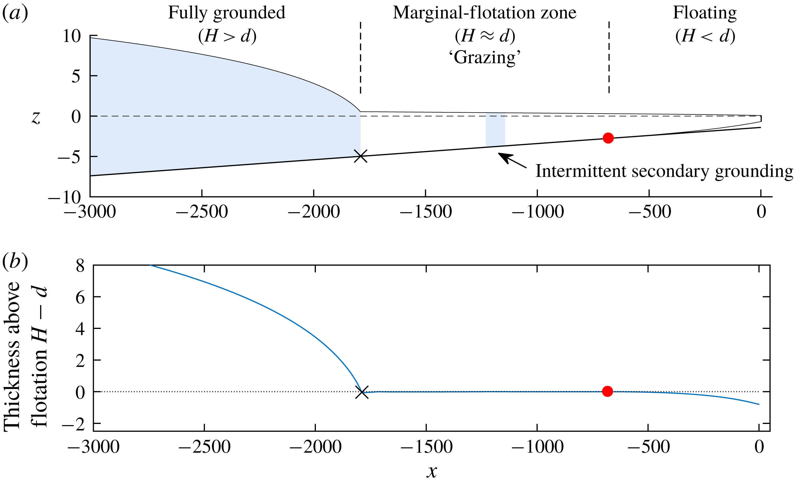
Panel (a) shows the three-component structure of a marine ice sheet, predicted by the numerical solution to the full system (2.17)–(2.21) for the example
 $\unicode[STIX]{x1D6FC}=2\times 10^{-3}$
,
 $\unicode[STIX]{x1D6FD}=1.4$
and
 $x_{D}=-3000$
, shown at time
 $t=7.5\times 10^{4}$
. Grounded sections of the flow are shown shaded. Panel (b) shows the difference
 $H(x,t)-d(x)$
, which distinguishes the three components of the marine ice sheet: the fully grounded region,
 $H>d$
, the fully floating region,
 $H<d$
, and, connecting them, the marginal-flotation zone, through which the thickness straddles the flotation thickness,
 $H\approx d$
. The black cross and red circle mark the edges of the marginal-flotation zone.
4.2.2 The marginal-flotation regime
The intermittent contacts between the ice shelf and the bedrock produce a distinctive flow regime referred to as ‘marginal flotation’. The regime is characterised by slight modulations in thickness that produce temporarily grounded regions over a well-defined interval intermediate to the fully grounded and fully floating regions. The overall structure of the flow is illustrated in figure 6(a). Here, the grounded regions are shown by blue shading, illustrating the firmly grounded region upstream, as well as a patch of temporarily grounded ice further downstream. A plot of
 $H(x,t)-d(x)$
in figure 6(b) clearly indicates the three-component structure of the ice sheet. A fully grounded region upstream, wherein
 $H>d$
, a fully floating region downstream, wherein
 $H<d$
, and an intermediate zone in which the thickness straddles the flotation thickness,
 $$\begin{eqnarray}H\approx d(x)\quad (\text{marginal flotation}).\end{eqnarray}$$
This region is referred to as the ‘marginal-flotation zone’.
The marginal-flotation zone represents a tertiary component of a marine ice sheet, additional to the fully grounded and fully floating regions. In essence, it replaces the notion of a grounding line with a grounding area, with the transition between floating and grounded regions taking place over an extended region. It is possible that regions of the WAIS may lie in this marginal-flotation state, which may appear in the form of distributed grounding zones or ice planes. Since the present-day WAIS is likely to be in a state of decline, such regions may not be widespread; as noted above, the development of this region is a hallmark of a grounding line recovering from tipped retreat. The prediction is a fundamental feature of ice-sheet dynamics that may be important in understanding the formation of ice sheets on time scales of glaciation and their potential to recover following tipping.
The patterns of grounding and detachment in the marginal-flotation zone, as predicted by the numerical solution, take the form of travelling waves, which begin at the downstream end of the marginal-flotation zone and propagate to the ‘primary’ grounding line at the upstream end of the marginal-flotation zone. The merging events of the grounded wave to the fully grounded region at the primary grounding line produce the oscillations shown in the inset of figure 5(b). The phenomenon of intermittent grounding represents a remarkable feature of the model, namely, that once the interior of the ice shelf grounds, the switch in the governing equation (2.17) leads to a new force balance that immediately favours its detachment from the base. Reducing the time step was thus found to increase the frequency of the switches and hence the frequency of the grounded pulses. The time-averaged predictions of the model (averaged over a few periods of the numerical oscillation, for example) are unchanged to leading order in small time step, indicating that the long-term migration predicted by the model within this regime is likely to be physically meaningful.
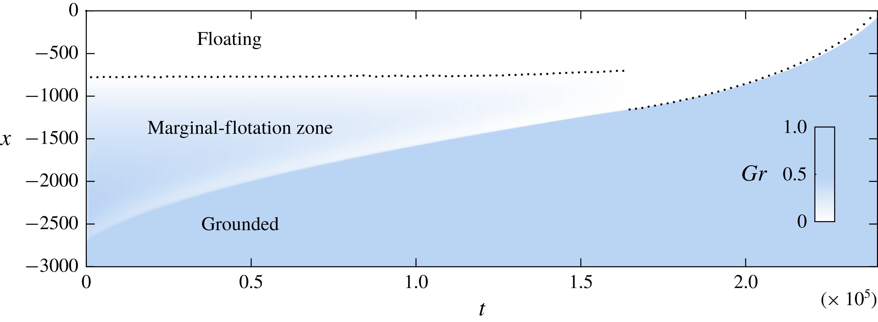
In order to investigate the structure of the marginal-flotation zone, I evaluate the time-averaged indicator function
 $$\begin{eqnarray}Gr(x,t)=\frac{1}{2T}\int _{t-T}^{t+T}1_{\{H(x,\unicode[STIX]{x1D70F})>d(x)\}}\,\text{d}\unicode[STIX]{x1D70F},\end{eqnarray}$$
where the integrand is equal to unity if the ice sheet is grounded and zero if it is floating, and
 $T$
is a specified time scale assumed smaller than the time scales on which the primary grounding line migrates. The variable
 $Gr(x,t)$
quantifies the proportion of time that a given point on the ice sheet lies grounded over the time interval
 $[t-T,t+T]$
. For a fully grounded or floating region,
 $Gr$
equals unity and zero, respectively, and intermediate values represent marginal flotation. The value of
 $Gr(x,t)$
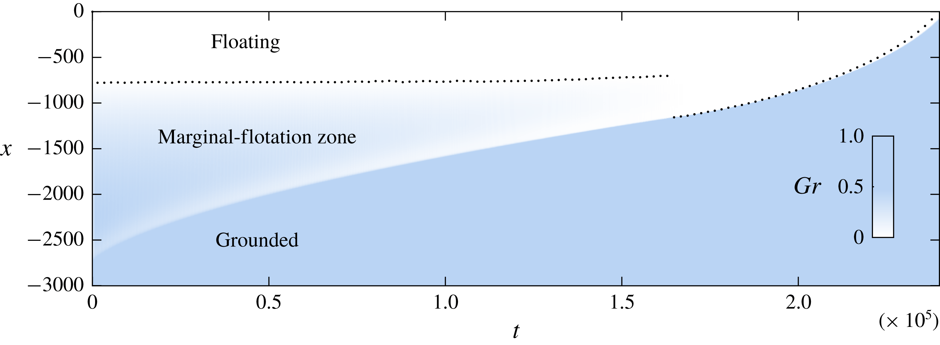
is shown as a density plot in figure 7 for the example of figure 5(b) and
 $T=500$
. The plot shows that the upstream boundary of the marginal-flotation zone, i.e. the ‘primary’ grounding line, gradually advances while the downstream boundary remains approximately constant. Perhaps surprisingly, the transition from
 $Gr=1$
to 0 does not occur monotonically; there is a band of relatively less grounding in front of the primary grounding line compared to the interior of the marginal-flotation zone (this structure mirrors that of the thickness profile of a confined ice shelf, which involves a region of rapid thinning in an extensional boundary layer in front of the grounding line; Pegler Reference Pegler2016). The marginal-flotation zone vanishes at
 $t=6.5\times 10^{4}$
, with a sharp transition between the fully grounded and floating regions persisting subsequently.
4.2.3 The case
$\unicode[STIX]{x1D6FD}/\unicode[STIX]{x1D6FD}_{0}>1$

I now address the qualitatively different case
 $\unicode[STIX]{x1D6FD}>\unicode[STIX]{x1D6FD}_{0}$
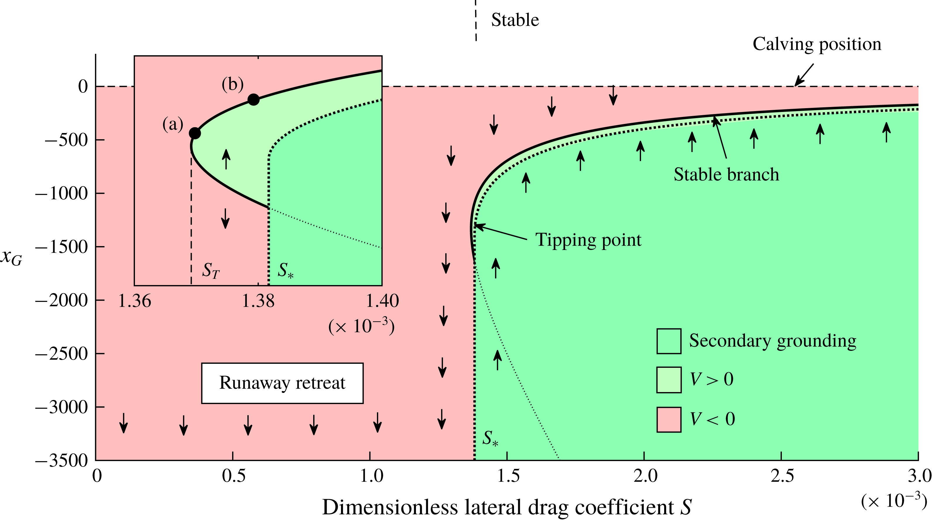
. The stability diagram for
 $\unicode[STIX]{x1D6FC}=2\times 10^{-3}$
and the deeper reference ocean depth
 $\unicode[STIX]{x1D6FD}=2.8>\unicode[STIX]{x1D6FD}_{0}$
is shown in figure 8. In contrast to the case
 $\unicode[STIX]{x1D6FD}<\unicode[STIX]{x1D6FD}_{0}$
, no steady state is possible if
 $S=0$
, in which case the unbuttressed grounding line would retreat unconditionally. As
 $S$
is increased, this conclusion continues to hold up to a critical value
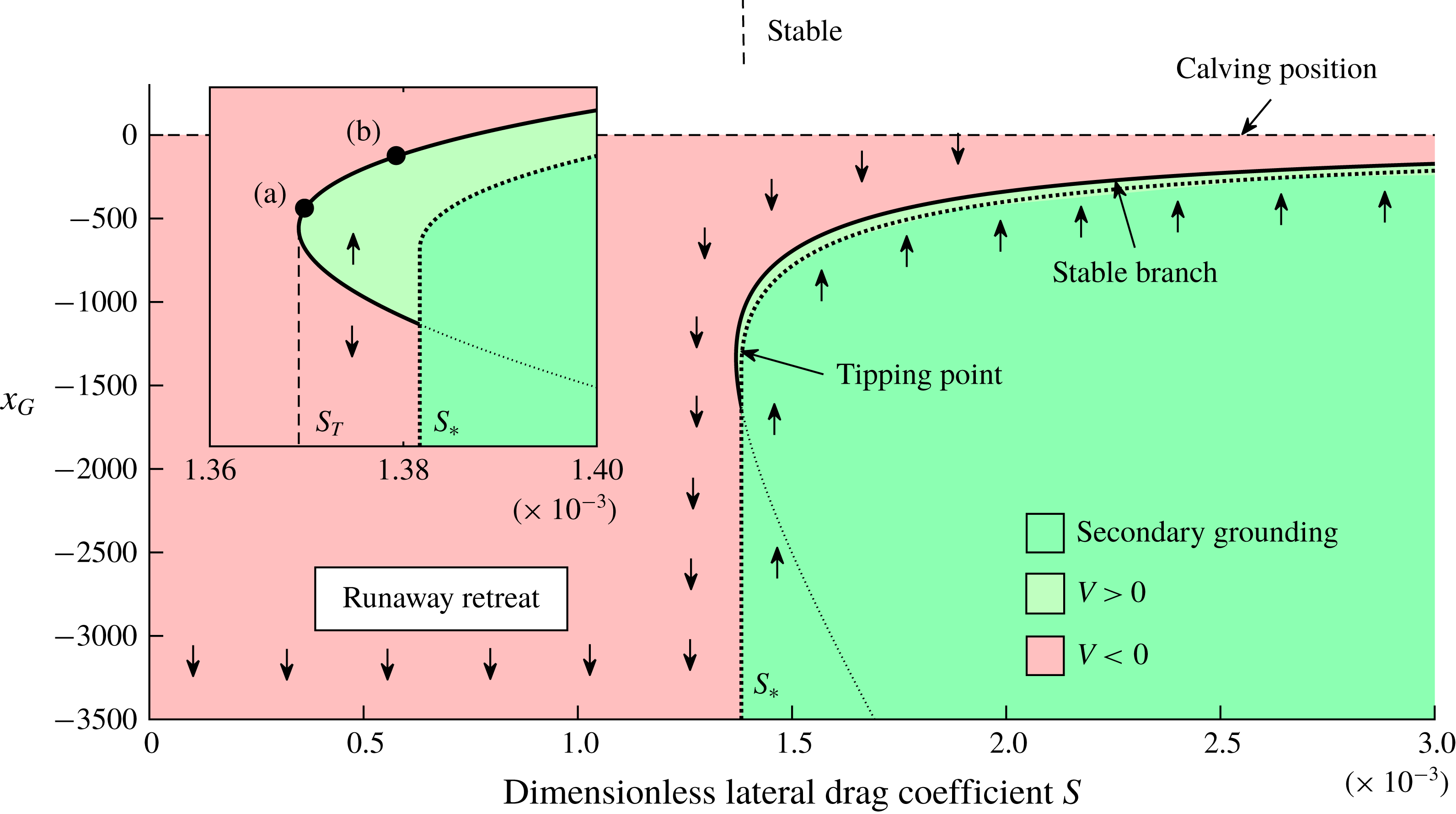
 $S_{T}(\unicode[STIX]{x1D6FC},\unicode[STIX]{x1D6FD})\approx 1.369\times 10^{-3}$
, whereat two steady states – one stable, the other unstable – appear at
 $x_{T}\approx -1330$
. As
 $S$
is increased further, the stable state moves downstream and the unstable state moves upstream. At a slightly larger value
 $S_{\ast }=1.382\times 10^{-3}$
, secondary grounding abruptly invalidates the unstable steady state, and completely covers the upstream region for which
 $V<0$
. A single, unconditionally stable steady state then remains. In regard to the contributions to the terms in the numerator of (3.3), the critical value
 $S_{T}$
represents the threshold at which the negative-feedback effect of ice-shelf buttressing can critically cancel the positive-feedback effects of buoyancy and extensional stress, creating a new stable steady-state branch along the interior of a positive bed slope.
The evolution of the grounding number
 $Gr(x,t)$
defined by (4.3), which measures the proportion of time that a region of the ice sheet lies grounded over a time scale of
 $T=500$
. The fully grounded region is represented by
 $Gr=1$
, the fully floating region by
 $Gr=0$
, and the marginal-flotation zone by
 $0<Gr<1$
. The end of the marginal-flotation zone is illustrated by a dotted curve. The extent of the zone reduces over time until it vanishes at
 $t\approx 1.65\times 10^{5}$
to leave a sharp transition between fully grounded and fully floating regions. Surprisingly. the transition from floating to grounding does not occur monotonically, with a local minimum in
 $Gr$
indicated by the relatively lighter band just downstream of the grounding line.
The stability diagram for the positive bed slope
 $\unicode[STIX]{x1D6FC}=2\times 10^{-3}$
and the reference ocean depth
 $\unicode[STIX]{x1D6FD}=2.8>\unicode[STIX]{x1D6FD}_{0}$
shown as a continuous variation of the drag parameter
 $S$
. Colour indicates the value of the stability variable
 $V(x)$
defined by (3.3) and the dark green region with a dashed outline represents the region of secondary grounding. Grounding-line retreat occurs unconditionally below a critical value
 $S_{T}(\unicode[STIX]{x1D6FC},\unicode[STIX]{x1D6FD})=1.369\times 10^{-3}$
. At
 $S=S_{T}$
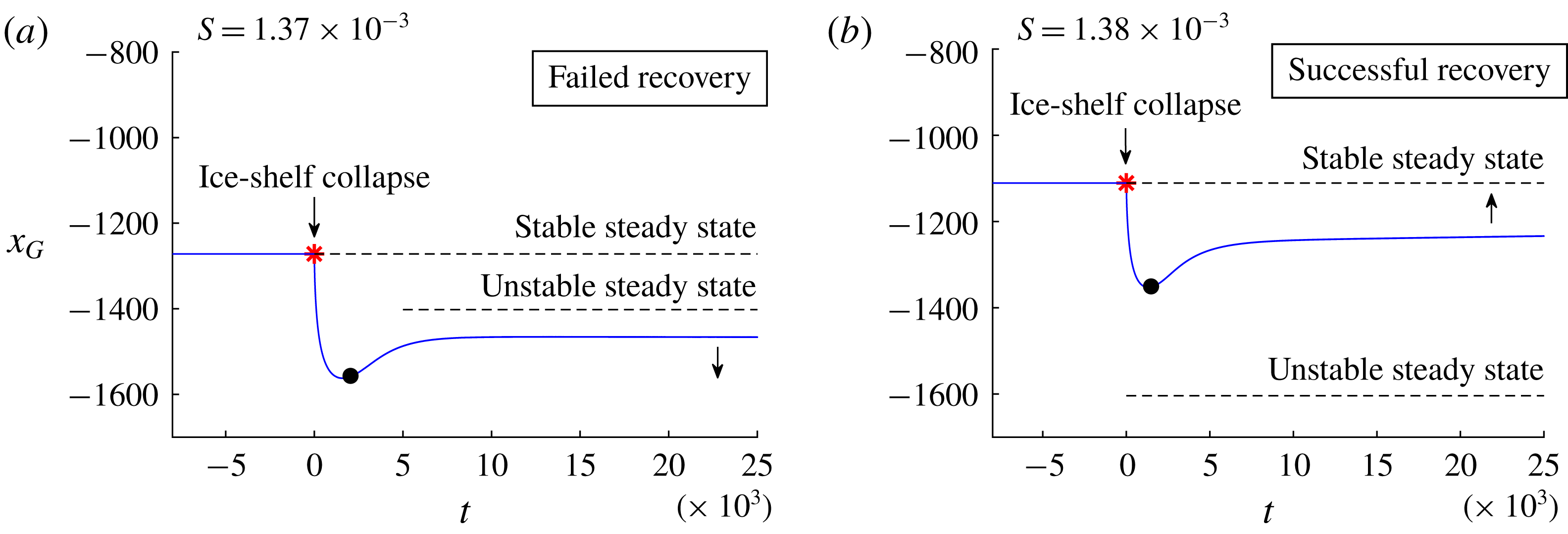
, two steady arise (one stable, the other unstable), as illustrated in the enlargement. The circular markers in this inset indicate the initial grounding-line positions for the computations following ice-shelf collapse of figure 9. At the slightly larger value
 $S_{\ast }(\unicode[STIX]{x1D6FC},\unicode[STIX]{x1D6FD})=1.382\times 10^{-3}$
, secondary grounding invalidates the unstable steady state and suppresses the possibility of runaway grounding-line retreat. Above
 $S_{\ast }$
, unconditional stabilisation towards the steady state occurs.
The branch of stable steady states is a new property of the stability diagram compared to
 $\unicode[STIX]{x1D6FD}<\unicode[STIX]{x1D6FD}_{0}$
that is inherently dependent on ice-shelf buttressing. A conclusion from § 4.2.1 illustrated in figure 4 is that there is no stable steady state possible if
 $\unicode[STIX]{x1D6FD}<\unicode[STIX]{x1D6FD}_{0}$
for all values of
 $S$
. By contrast, the stable steady states arising here for
 $\unicode[STIX]{x1D6FD}>\unicode[STIX]{x1D6FD}_{0}$
and
 $S>S_{T}$
are a robust long-term regime, indicating that the removal of such states as a consequence of parameter variation (e.g. reduction of the upstream flux
 $Q$
) provides the trigger to tipped retreat of a buttressed marine ice sheet. A key question is: how might a runaway grounding-line retreat be triggered if a marine ice sheet lies on the stable branch? One plausible trigger is the large-scale collapse of the ice shelf, which abruptly removes the buttressing force, and may provoke instability if the ice shelf fails to recover sufficiently quickly. Another mechanism for destabilisation is for parameters, such as the calving position or melt rate, to vary in time and cause a transition from supercriticality,
 $S>S_{T}(\unicode[STIX]{x1D6FC},\unicode[STIX]{x1D6FD})$
, to subcriticality,
 $S<S_{T}(\unicode[STIX]{x1D6FC},\unicode[STIX]{x1D6FD})$
. The stability diagram of figure 8 indicates that such a transition would involve an initially quasi-steady migration along the stable branch followed by a sudden onset of tipped grounding-line retreat upstream of the critical ‘cliff edge’ grounding-line position
 $x_{T}$
.
Grounding-line evolutions following the collapse of the ice shelf for
 $\unicode[STIX]{x1D6FC}=2\times 10^{-3}$
,
 $\unicode[STIX]{x1D6FD}=2.8$
and
 $x_{D}=-3\times 10^{3}$
for (a)
 $S=1.37\times 10^{-4}$
and (b)
 $S=1.38\times 10^{-4}$
, obtained from the numerical solution of the full equations (2.17)–(2.21). Each computation is initialised from the stable steady state, corresponding to the positions of the circular markers in the inset of figure 8. In case (a), the grounding line initially retreats upstream of the unstable steady state and ultimately fails to recover to the original steady state. The time at which the front of the ice shelf reaches its former calving position,
 $x_{C}(t)=0$
, is indicated by a filled circle. In case (b), the grounding line instead remains downstream of the unstable steady state and a long-term recovery ensues. The results show that an ice-shelf collapse generally leads to total restoration of the marine ice sheet for even marginally supercritical values of
 $S>S_{\ast }$
.
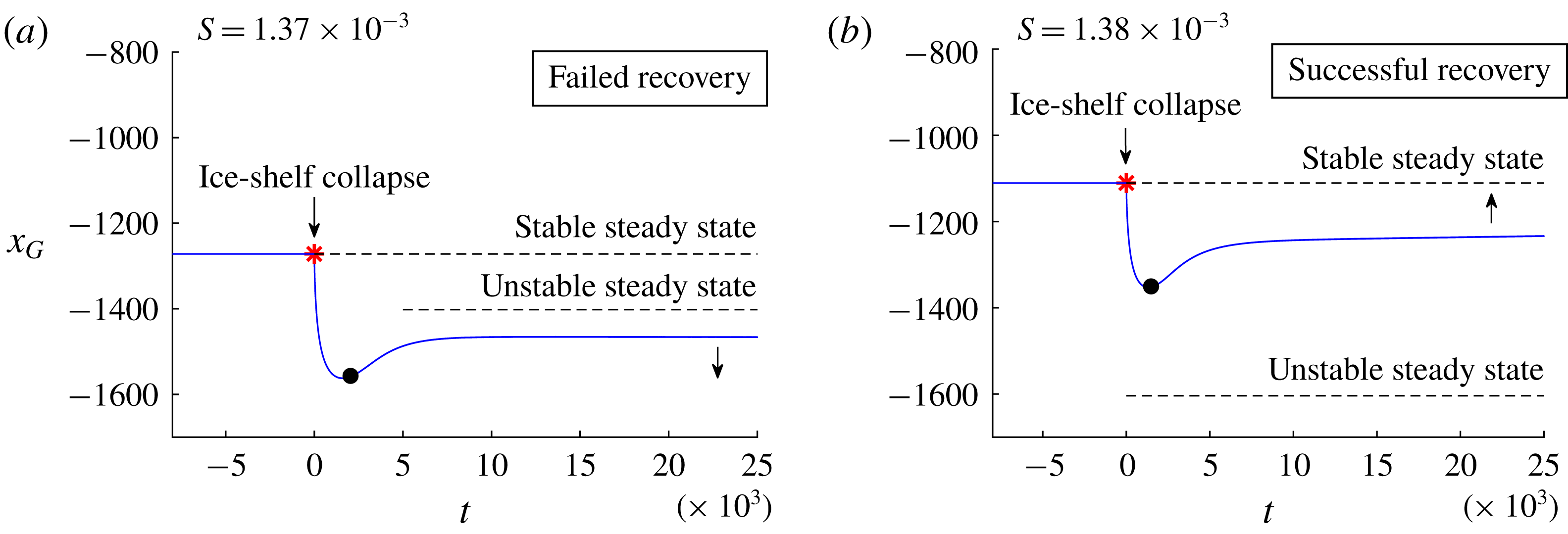
In order to investigate the first possibility of destabilisation from ice-shelf collapse, I ran a series of time-dependent computations initialised at a selection of positions along the stable branch. In each case, I removed the ice shelf completely at
 $t=0$
. Subsequently, the front of the ice shelf was evolved with the flow rate until it recovered to the position
 $x_{C}$
, beyond which time the calving front was again imposed at
 $x_{C}$
. It was found that the grounding line recovers in all cases, with the exception of a range of
 $S$
very close to the critical value
 $S_{T}\approx 1.369$
. The results for two marginally supercritical critical values of
 $S$
given by
 $S=1.370\times 10^{-3}$
and 1.380
 $\times 10^{-3}$
are illustrated in panels (a) and (b) of figure 9, respectively. For case (a), the removal of the ice shelf leads to a relatively sudden retreat of the grounding line to a minimum position at
 $t\approx 1500$
. Near this minimum, the front of the ice shelf reaches its former calving position, indicated by a filled circular marker. Following this, the grounding line remains upstream of the unstable steady state and long-term recovery fails. For case (b), the initial retreat of the grounding line instead remains downstream of the unstable steady state indicated by a dashed line, which is consistent with a long-term recovery to the original steady state. It should be noted that the range of values of
 $S$
for which recovery fails is extremely limited to situations very close to
 $S_{T}$
: all values of
 $S>1.001\,S_{T}$
undergo a complete recovery.
In light of the results above, I would anticipate that the destabilisation of a marine ice sheet from a buttressed steady state is more likely to arise from parametric variation in the properties of the ice sheet inducing a transition from supercriticality
 $S>S_{T}$
to subcriticality
 $S<S_{T}$
. This transition has the character of a ‘cliff-edge’, with robust stability occurring for
 $S>S_{T}$
to a sudden loss of local stability occurring for
 $S<S_{T}$
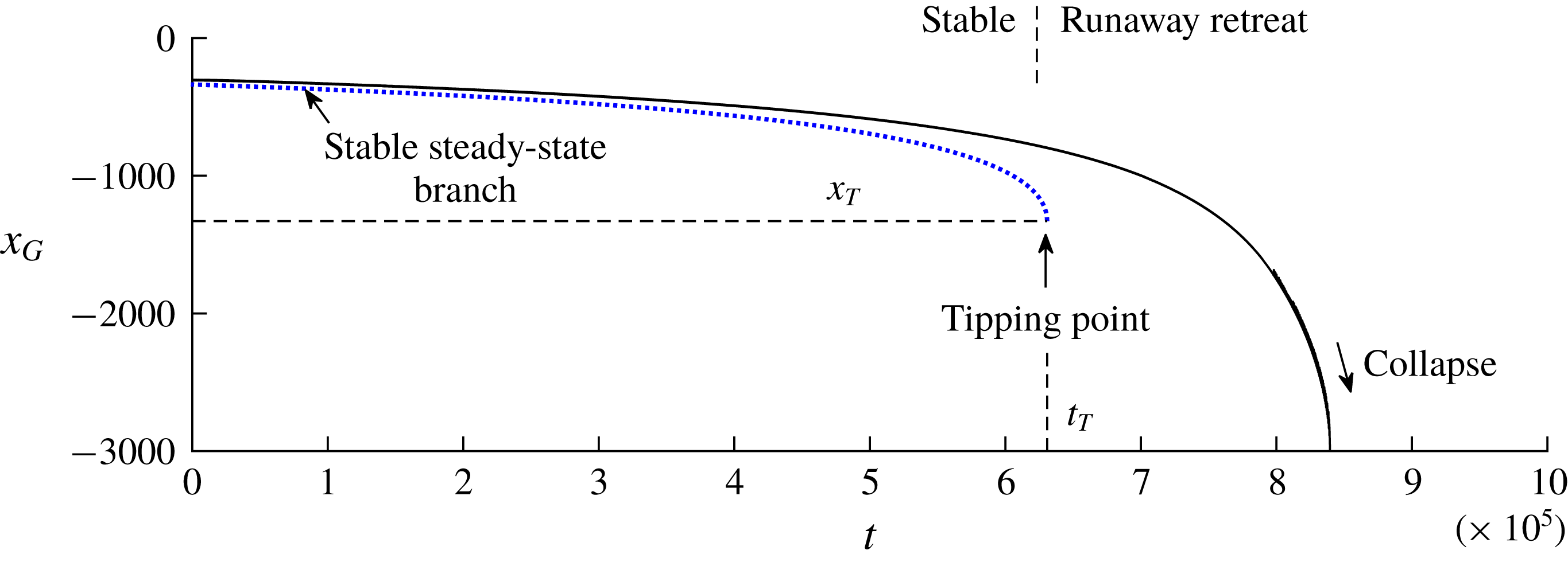
. To illustrate this mode of destabilisation, I ran a computation in which the parameter
 $S=S(t)$
is ramped down linearly from the supercritical value
 $S=2\times 10^{-3}>S_{T}$
to the subcritical value
 $10^{-3}<S_{T}$
over a time scale of
 $t=10^{6}$
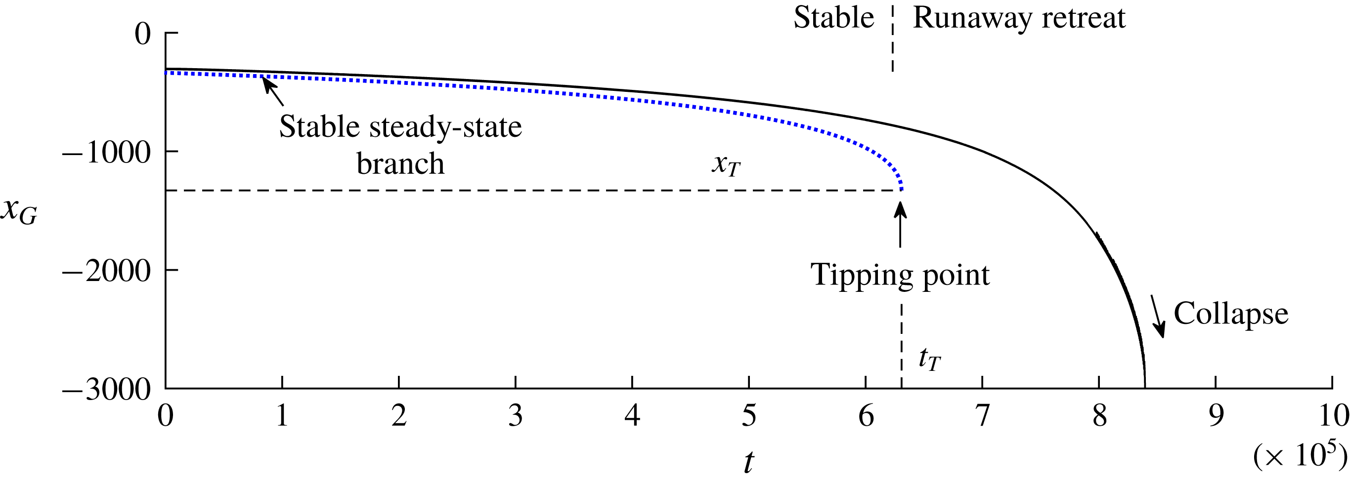
, shown in figure 10. Initially, the grounding line retreats in proximity to the stable branch of steady states shown by a blue dotted curve in a quasi-steady manner, representing ‘stable’ retreat. Once the threshold
 $S_{T}$
is passed at
 $t=t_{T}\approx 6.3\times 10^{5}$
, a relatively rapid ‘tipped’ grounding-line retreat ensues, culminating in detachment of the ice sheet a relatively short time later at
 $t\approx 8.4\times 10^{5}$
whereat
 $x_{G}=x_{D}$
. More than 80 % of the retreat with respect to the initial position occurs for
 $t>t_{T}$
, confirming that the critical value
 $S_{T}$
represents a tipping point. Thus, while the ice sheet is totally secure for even marginally supercritical values of
 $S>S_{T}$
(against even a full ice-shelf collapse), security vanishes completely below the threshold
 $S_{T}$
.
The grounding-line evolution
 $x_{G}(t)$
following initialisation at the stable steady state for
 $S=2\times 10^{-3}>S_{T}$
,
 $\unicode[STIX]{x1D6FC}=2\times 10^{-3}$
,
 $\unicode[STIX]{x1D6FD}=2.8$
, and
 $x_{D}=-3\times 10^{3}$
and a gradual ramping down of the lateral drag parameter
 $S=S(t)$
to the subcritical value
 $S=10^{-3}<S_{T}$
linearly over a time scale of
 $t=10^{6}$
. The plot illustrates the initial quasi-steady migration along the stable branch given by the solution to (3.1) shown as a dotted blue curve, followed by the onset of a runaway grounding-line retreat beyond the ‘cliff-edge’ at which the steady branch terminates. The critical transition to instability occurs once
 $S(t)>S_{T}\approx 1.36\times 10^{-3}$
or
 $t>t_{T}\approx 6.3\times 10^{5}$
.
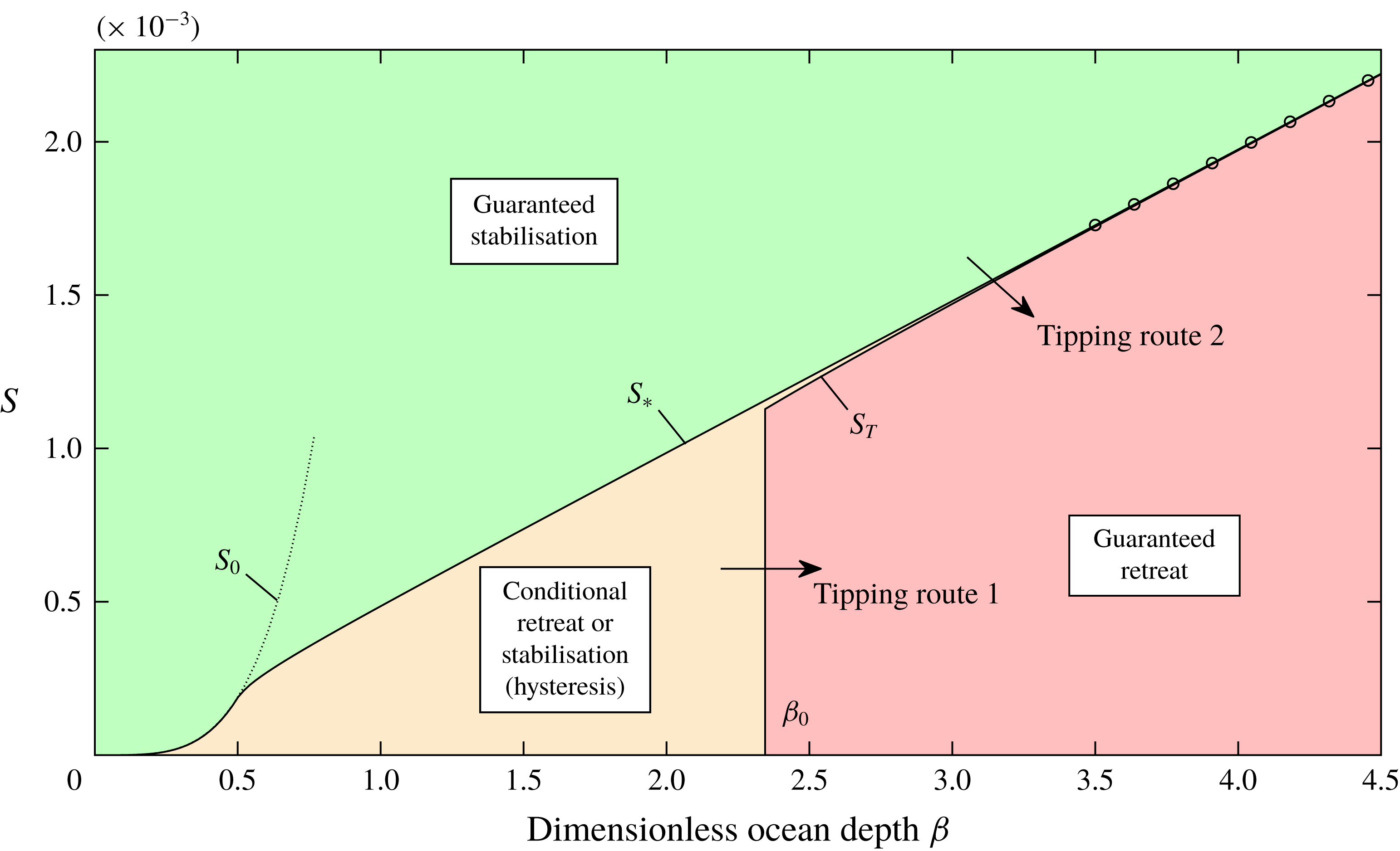
Regime diagram illustrating the conditions for stability of a buttressed marine ice sheet on a retrograde slope across the space of dimensionless reference ocean depth
 $\unicode[STIX]{x1D6FD}$
and lateral drag coefficient
 $S$
. The dimensionless slope
 $\unicode[STIX]{x1D6FC}=2\times 10^{-3}$
is illustrated, and is representative of the general case. If
 $S>S_{\ast }$
(green), the system is guaranteed to remain stable for any dimensionless ocean depth. If
 $S<S_{\ast }$
and
 $\unicode[STIX]{x1D6FD}<\unicode[STIX]{x1D6FD}_{0}\approx 2.345$
(yellow) then stabilisation is contingent on whether the grounding line lies downstream of the unstable steady state. If
 $S<S_{\ast }$
and
 $\unicode[STIX]{x1D6FD}>\unicode[STIX]{x1D6FD}_{0}$
then there is a very narrow range
 $S_{T}<S<S_{\ast }$
for which stability is also contingent on the grounding line lying downstream of the unstable steady state (yellow). Otherwise, runaway grounding-line retreat is guaranteed (red). The approximation for the critical tipping-point value of
 $S_{\ast }$
given by (5.5) is shown as a line of circular markers. The critical value of
 $S_{0}$
given by (5.3) for which the calving front is predicted to contact the bedrock for
 $S<S_{0}$
is shown as a dotted black curve. The arrows indicate the two different pathways for instigation of instability, as given by the two criteria (5.7) and (5.8).
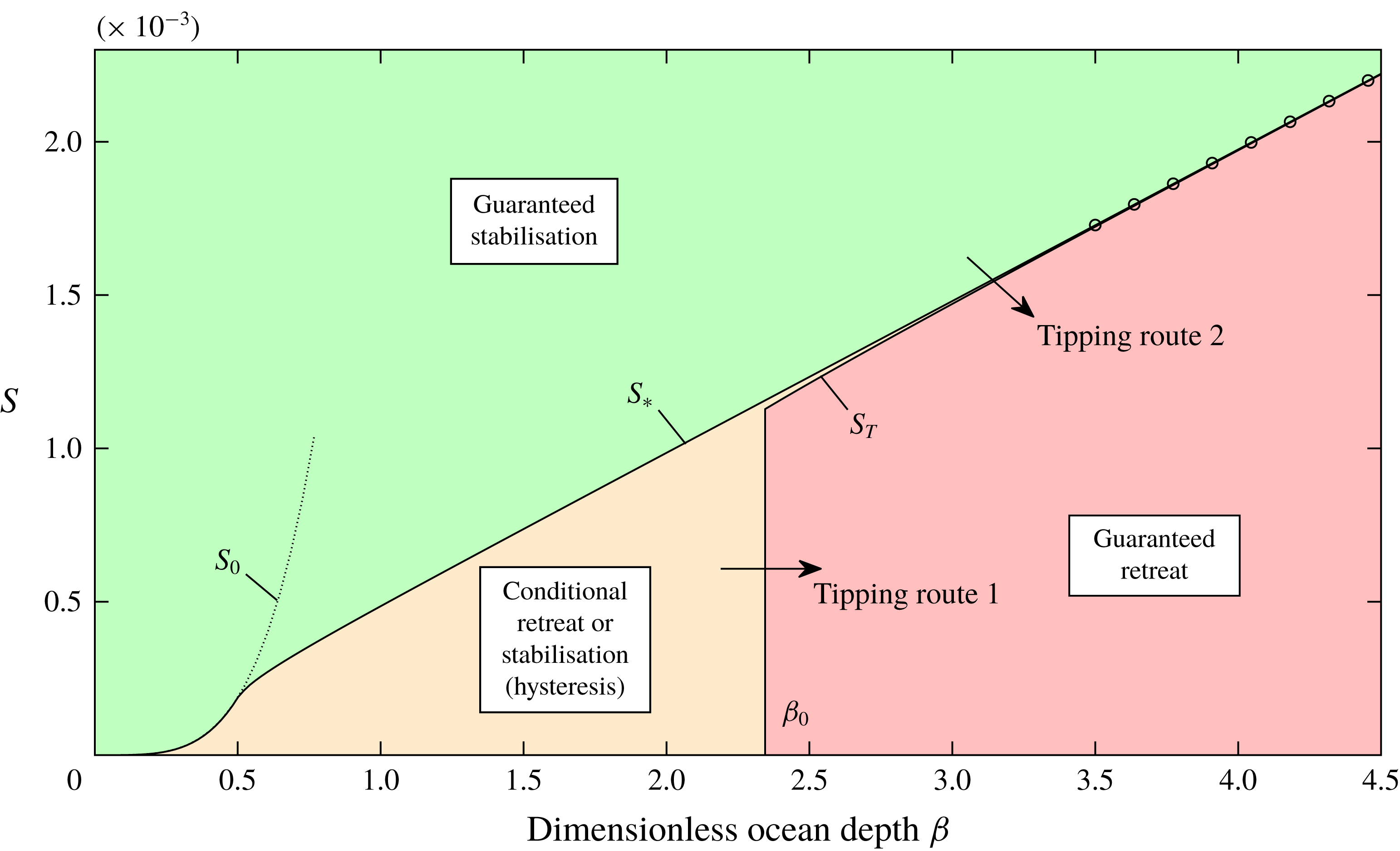
5 Thresholds for tipping and recovery of a marine ice sheet
The general conditions for stability of a marine ice sheet on a retrograde slope are shown in figure 11. Here, I plot the critical dimensionless lateral drag coefficients,
 $S_{\ast }(\unicode[STIX]{x1D6FC},\unicode[STIX]{x1D6FD})$
and
 $S_{T}(\unicode[STIX]{x1D6FC},\unicode[STIX]{x1D6FD})$
, for the illustrative case
 $\unicode[STIX]{x1D6FC}=2\times 10^{-3}$
as a function of
 $\unicode[STIX]{x1D6FD}$
, which provide the critical boundaries of the possible regimes. For
 $S>S_{T}$
, the inducement of secondary grounding guarantees the stability of the ice sheet (the green region). For
 $S<S_{\ast }$
, secondary grounding cannot suppress the retreat, and the stability depends on the dimensionless ocean depth
 $\unicode[STIX]{x1D6FD}$
. In this case, if
 $\unicode[STIX]{x1D6FD}<\unicode[STIX]{x1D6FD}_{0}\equiv (1-\unicode[STIX]{x1D6FF})d_{0}$
(the yellow region), runaway grounding-line retreat occurs if the grounding line lies upstream of the unstable steady state. For
 $\unicode[STIX]{x1D6FD}>\unicode[STIX]{x1D6FD}_{0}$
, runaway grounding-line retreat is guaranteed (the red region) with the exception of a very narrow band
 $S_{T}<S<S_{\ast }$
of values where retreat is conditional on the grounding line lying upstream of the unstable steady state. The plot shows that the transition to tipped retreat from a buttressed steady state generally occurs abruptly across a parametric threshold. For the unbuttressed case, a transition to runaway retreat can occur only if
 $\unicode[STIX]{x1D6FD}$
changes from less than
 $\unicode[STIX]{x1D6FD}_{0}$
to greater than
 $\unicode[STIX]{x1D6FD}_{0}$
. A transition from buttressed stability also depends on a transition from
 $S>S_{T}$
to
 $S<S_{T}$
, representing a stability criterion that is entirely distinct from the transition associated with unbuttressed MISI. Subsequent recovery of the grounding line depends on
 $S$
increasing to the slightly larger value
 $S_{\ast }\gtrsim S_{T}$
.
For a general topography
 $b(x)$
and calving position, the ‘tipping point’ critical values of
 $S$
can be defined by


These represent the minimum value of
 $S$
for which a stable steady state exists, and the minimum value of
 $S$
such that secondary grounding occurs in steady state, respectively. The stability of the ice sheet is critically removed once
 $S$
drops below
 $S_{T}$
. In practice, it is possible for there to be multiple localised tipping points (each a saddle-node bifurcation), and these will be illustrated by the stability diagram constructed for a given scenario. In such cases, transitioning across a tipping point may cause the grounding line to migrate to a new steady state upstream. The value of (5.1) represents the final tipping point below which the system will continue to retreat without subsequently stabilising towards a new steady state.
The plot of figure 11 indicates that the two critical values
 $S_{T}$
and
 $S_{\ast }$
are numerically almost coincident. This coincidence occurs because both values occur close to the location where the lateral-drag-dominated section of the ice shelf intersects the bedrock (Pegler Reference Pegler2018). In order to confirm that
 $S_{\ast }$
and
 $S_{T}$
are approximately coincident in general, I plot these functions for a range of bed slopes
 $\unicode[STIX]{x1D6FC}=2\times 10^{-4},2\times 10^{-3},2\times 10^{-2}$
, in figure 12 (spanning three orders of magnitude). The plot shows that
 $S_{T}$
(solid) and
 $S_{\ast }$
(dotted) practically coincide in each case. Note that
 $S_{T}$
is only defined for
 $\unicode[STIX]{x1D6FD}>\unicode[STIX]{x1D6FD}_{0}$
because it represents the critical turning point of the branch of stable steady states, which only exists for
 $\unicode[STIX]{x1D6FD}>\unicode[STIX]{x1D6FD}_{0}$
.
It should be noted that there is a special region of the parameter space,
 $S<S_{0}(\unicode[STIX]{x1D6FD})$
, for which the calving front of the ice shelf itself is predicted to penetrate the bedrock (as opposed to the interior to the ice shelf). For these special situations, the critical cotangency conditions for secondary grounding (3.5) are not applicable and, instead, the condition for secondary grounding is
 $H_{C}>\unicode[STIX]{x1D6FD}$
. Using the analytical prediction for the calving-front thickness for
 $n=1$
, namely,
 $H_{C}=\unicode[STIX]{x1D705}(S/\unicode[STIX]{x1D6FF}^{2})^{1/4}$
, where
 $\unicode[STIX]{x1D705}\approx 1.502$
(Pegler Reference Pegler2016), I determine this critical value as
 $$\begin{eqnarray}S_{0}=\unicode[STIX]{x1D6FF}^{2}\{\unicode[STIX]{x1D6FD}/[\unicode[STIX]{x1D705}(1-\unicode[STIX]{x1D6FF})]\}^{4},\end{eqnarray}$$
which is shown by the thin dotted curves in figures 11 and 12. The value
 $S_{0}$
represents the termination of the threshold value
 $S_{\ast }$
for which cotangency is possible, as illustrated in figure 12.
To gain analytical insight into the nature of the buttressed stability criterion
 $S>S_{\ast }(\unicode[STIX]{x1D6FC},\unicode[STIX]{x1D6FD})$
, and its parametric form, I determine an analytical approximation for
 $S_{\ast }(\unicode[STIX]{x1D6FC},\unicode[STIX]{x1D6FD})$
. As discussed in Pegler (Reference Pegler2018), the critical cotangency condition for secondary grounding (3.5) is given approximately by the strong-buttressing limiting balance of (3.1), namely,
 $$\begin{eqnarray}{\textstyle \frac{1}{2}}\unicode[STIX]{x1D6FF}d(x_{G})^{2}\approx B(x_{G},x_{C}).\end{eqnarray}$$
Substituting (3.2b
) into (5.4), and rearranging for
 $S$
, I determine the threshold value
 $$\begin{eqnarray}\displaystyle S_{\ast } & {\approx} & \displaystyle \min _{x}\left[{\textstyle \frac{1}{2}}\unicode[STIX]{x1D6FF}d(x)^{2}/(x_{C}-x)\right],\end{eqnarray}$$
 $$\begin{eqnarray}\displaystyle & = & \displaystyle 2\unicode[STIX]{x1D6FF}(1-\unicode[STIX]{x1D6FF})^{-2}\unicode[STIX]{x1D6FC}\unicode[STIX]{x1D6FD}\end{eqnarray}$$
for the linear bedrock. The analytical approximation (5.6) is shown as a line of circular markers in figure 11 and is confirmed to provide excellent agreement with the numerical result. The result implies a near linear relationship between
 $S_{\ast }$
and the basal slope
 $\unicode[STIX]{x1D6FC}$
and the reference depth
 $\unicode[STIX]{x1D6FD}$
.
The critical values of the dimensionless lateral shear drag coefficients,
 $S_{T}$
(solid black curve) and
 $S_{\ast }$
(dotted blue curve), representing the terminus of the stable branch of steady states and of the instance of secondary grounding, respectively, plotted against the reference ocean depth
 $\unicode[STIX]{x1D6FD}$
for bed slopes
 $\unicode[STIX]{x1D6FC}=2\times 10^{-4}$
,
 $2\times 10^{-3}$
and
 $2\times 10^{-2}$
, spanning two orders of magnitude. The plot illustrates the approximate equivalence of
 $S_{T}$
and
 $S_{\ast }$
across the complete parameter space. The critical dimensionless ocean depth
 $\unicode[STIX]{x1D6FD}_{0}$
for which the stable branch exists for
 $\unicode[STIX]{x1D6FD}>\unicode[STIX]{x1D6FD}_{0}$
is shown as a vertical dashed line. The critical value of
 $S_{0}$
given by (5.3) for which the calving front of the ice shelf is predicted to contact the bedrock is shown as a thin dotted curve, and provides the minimum of
 $S_{\ast }$
for each value of
 $\unicode[STIX]{x1D6FC}$
.

The result of (5.6) yields an analytical condition for grounding-line stability,
 $S<S_{\ast }(\unicode[STIX]{x1D6FC},\unicode[STIX]{x1D6FD})$
. A transition to tipped retreat will therefore occur, for example, if the flux
 $Q$
reduces sufficiently for the threshold
 $S=S_{\ast }$
to become crossed. In discussing the critical transitions from a stable ice sheet to tipped retreat, I henceforth assume that the topography downstream of the reference position
 $x=0$
slopes downwards, such that there is a topographic maximum at
 $x=0$
and
 $\unicode[STIX]{x1D6FD}$
is the minimum ocean depth. For the context of an unbuttressed grounding line, a transition from a stable configuration on the downwards slope for
 $x>0$
to a positive slope for
 $x<0$
occurs critically once the dimensionless reference depth
 $\unicode[STIX]{x1D6FD}$
drops below the value
 $\unicode[STIX]{x1D6FD}_{0}$
. In the general buttressed context, there are instead two distinct criteria necessary to trigger instability in this configuration, namely, both
 $\unicode[STIX]{x1D6FD}>\unicode[STIX]{x1D6FD}_{0}$
and
 $S<S_{T}$
. In their dimensional forms, these criteria read
 $$\begin{eqnarray}\displaystyle Q & {<} & \displaystyle \frac{\unicode[STIX]{x1D70C}g}{\unicode[STIX]{x1D707}_{0}}\left[\frac{\unicode[STIX]{x1D6FF}\unicode[STIX]{x1D707}_{0}}{8C_{-}}\left(\frac{|b_{0}|}{1-\unicode[STIX]{x1D6FF}}\right)^{5}\right]^{1/2}\quad (\text{tipping criterion 1}),\end{eqnarray}$$
 $$\begin{eqnarray}\displaystyle Q & {<} & \displaystyle \frac{2\unicode[STIX]{x1D70C}g^{\prime }a|b_{0}|w}{(1-\unicode[STIX]{x1D6FF})^{2}C_{+}}\hspace{55.00008pt}\quad (\text{tipping criterion 2}),\end{eqnarray}$$
respectively. These two distinct necessary criteria for transitioning to tipped grounding-line retreat are illustrated by the arrows in the regime diagram of figure 11. Importantly, either one can provide the critical threshold for tipping, and each represents a different pathway in parameter space resulting in runaway retreat. For an unbuttressed grounding line,
 $C_{+}=0$
and criterion 2 is automatically satisfied. The only criterion for transition to instability is then criterion 1, which represents the threshold at which the thickness necessary for an unbuttressed steady-state grounding line to exist decreases below the minimum flotation thickness
 $|b_{0}|$
. Criterion 2 introduces a distinct tipping threshold controlled by ice-shelf buttressing. It is interesting that for
 $S<S_{\ast }(\unicode[STIX]{x1D6FD}_{0})$
, only criterion 1 is necessary for tipping. Over this region of the parameter space, the buttressing force, while present, plays no role in controlling the onset of tipping.
6 Tipping thresholds controlled by ice-shelf calving and melting
To this point, I have illustrated the onset of tipped retreat by variation of the dimensionless lateral shear-drag coefficient
 $S$
, a parameter grouping that is dependent in particular on snowfall accumulation
 $Q$
and channel width. Here, I will demonstrate other natural modes of transitioning to tipped retreat, namely, the retreat of the calving front of the ice shelf
 $x_{C}$
and an increase in the net rate of melting along the base of the ice shelf,
 $-f(x)$
, which will each erode the buttressing force generated by the ice shelf. The dynamics of a grounding line is, via the buttressing force, sensitive to both the melt-rate distribution and the control of its calving position (e.g. Dupont & Alley Reference Dupont and Alley2005; Gagliardini et al.
Reference Gagliardini, Durand, Zwinger, Hindmarsh and Meur2010; Nick et al.
Reference Nick, van der Veen, Vieli and Benn2010; Gudmundsson et al.
Reference Gudmundsson, Krug, Durand, Favier and Gagliardini2012; Gudmundsson Reference Gudmundsson2013; Favier et al.
Reference Favier, Durand, Cornford, Gudmundsson, Gagliardini, Gillet-Chaulet and Brocq2014; Schoof et al.
Reference Schoof, Davis and Popa2017). In particular, the possibility of a stable grounding line on a retrograde slope depends sensitively on the choice of calving model and its underlying parameters (Schoof et al.
Reference Schoof, Davis and Popa2017).
For illustrating the critical tipping points associated with changes in calving position and melt rate, I will first confirm that the same qualitative features of the stability–regime diagram of figure 11 also apply for the shear-thinning power-law exponent
 $n=3$
. Thus, I write the expressions for
 $E$
and
 $B$
given by (2.10) and (2.11), which take the dimensionless forms
 $$\begin{eqnarray}\displaystyle & \displaystyle E[d(x_{G})]=4d(x_{G})^{(n^{2}-3n-1)/n^{2}}, & \displaystyle\end{eqnarray}$$
 $$\begin{eqnarray}\displaystyle & \displaystyle B(x_{G})=\frac{\unicode[STIX]{x1D6FF}}{2}\left\{\!\left[\frac{N}{\unicode[STIX]{x1D6FF}}\int _{x_{G}}^{x_{C}}Sq(x^{\prime })^{1/n}\,\text{d}x^{\prime }+H_{C}^{N}\right]^{2/N}-H_{C}^{2}\right\}, & \displaystyle\end{eqnarray}$$
where
 $N\equiv (n+1)/n$
,
 $\tilde{H}_{C}\approx \unicode[STIX]{x1D705}\unicode[STIX]{x1D702}$
,
 $\unicode[STIX]{x1D702}\equiv \unicode[STIX]{x1D6FF}^{-1/N}S^{1/(nN^{2})}$
,
 $q=1-\int _{x_{G}}^{x}M(x)\,\text{d}x$
,
 $M(x)\equiv -f(x){\mathcal{L}}/Q$
is the dimensionless melt-rate distribution and I have again neglected here the contribution due to
 $\text{d}b/\text{d}x$
in
 $E$
.
Regime diagram illustrating the conditions for stability of a buttressed marine ice sheet on a retrograde slope across the space of dimensionless reference ocean depth
 $\unicode[STIX]{x1D6FD}$
and lateral drag coefficient
 $S$
for the power-law case
 $n=3$
. The diagram is the power-law analogue of figure 11. The dimensionless slope
 $\unicode[STIX]{x1D6FC}=2\times 10^{-4}$
is illustrated, and is representative of the general case. If
 $S>S_{\ast }$
(green), the system is guaranteed to remain stable for any dimensionless ocean depth. If
 $S<S_{\ast }$
and
 $\unicode[STIX]{x1D6FD}<\unicode[STIX]{x1D6FD}_{0}\approx 7.96$
(yellow) then stabilisation is contingent on whether the grounding line lies downstream of the unstable steady state. If
 $S<S_{\ast }$
and
 $\unicode[STIX]{x1D6FD}>\unicode[STIX]{x1D6FD}_{0}$
then there is a very narrow range
 $S_{T}<S<S_{\ast }$
for which stability is also contingent on the grounding line lying downstream of the unstable steady state (yellow). Otherwise, runaway grounding-line retreat is guaranteed (red). The approximation for the critical tipping-point value of
 $S_{\ast }$
given by (6.4) is shown as a line of circular markers. The critical value of
 $S_{0}$
given by (6.3) for which the calving front is predicted to contact the bedrock for
 $S<S_{0}$
is shown as a dotted black curve.
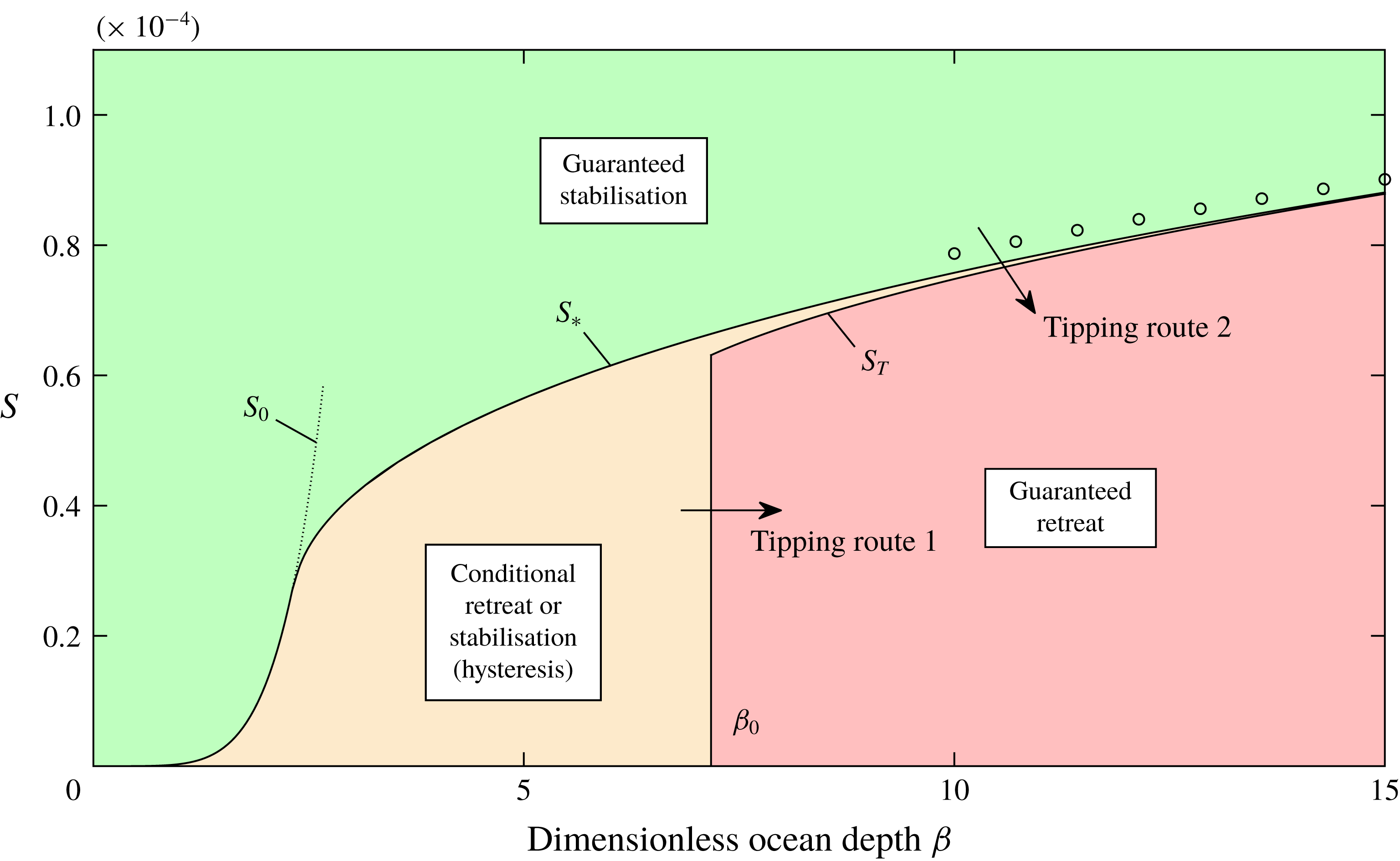
The regime diagram constructed for
 $n=3$
,
 $\unicode[STIX]{x1D6FC}=2\times 10^{-4}$
, zero melting
 $M=0$
and
 $x_{C}=0$
is shown in figure 13. The plot represents the power-law analogue of figure 11. As in the Newtonian case, there is a range of shallow slopes for which
 $S<S_{0}(\unicode[STIX]{x1D6FD})$
, where
 $$\begin{eqnarray}S_{0}(\unicode[STIX]{x1D6FD})=\unicode[STIX]{x1D6FF}^{n+1}(\unicode[STIX]{x1D6FD}/[\unicode[STIX]{x1D705}(1-\unicode[STIX]{x1D6FF})])^{nN^{2}},\end{eqnarray}$$
for which the calving front itself is predicted to intersect the bedrock. The regime diagram again shows the near coincidence of the critical values
 $S_{\ast }$
and
 $S_{T}$
. One difference compared to
 $n=1$
is that the critical values increase nonlinearly with
 $\unicode[STIX]{x1D6FD}$
. Repeating the analysis used to develop (5.6), one can determine the approximation
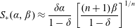 $$\begin{eqnarray}S_{\ast }(\unicode[STIX]{x1D6FC},\unicode[STIX]{x1D6FD})\approx \frac{\unicode[STIX]{x1D6FF}\unicode[STIX]{x1D6FC}}{1-\unicode[STIX]{x1D6FF}}\left[\frac{(n+1)\unicode[STIX]{x1D6FD}}{1-\unicode[STIX]{x1D6FF}}\right]^{1/n}\end{eqnarray}$$
which is shown as a curve of circular markers in figure 13, confirming the nonlinear dependence. The regime diagram illustrates the same properties as the regime diagram of figure 11 for
 $n=1$
, including the two different routes for tipping into MISI.
Stability diagrams illustrating the grounding-line position and critical transition to tipped retreat against (a) calving position
 $x_{C}$
and (b) melt rate
 $M$
. For these examples,
 $\unicode[STIX]{x1D6FC}=2\times 10^{-4}$
,
 $\unicode[STIX]{x1D6FD}=12$
and
 $S=10^{-4}$
. For (a), the melt rate
 $M=0$
. For (b), the calving position is
 $x_{C}=0$
.
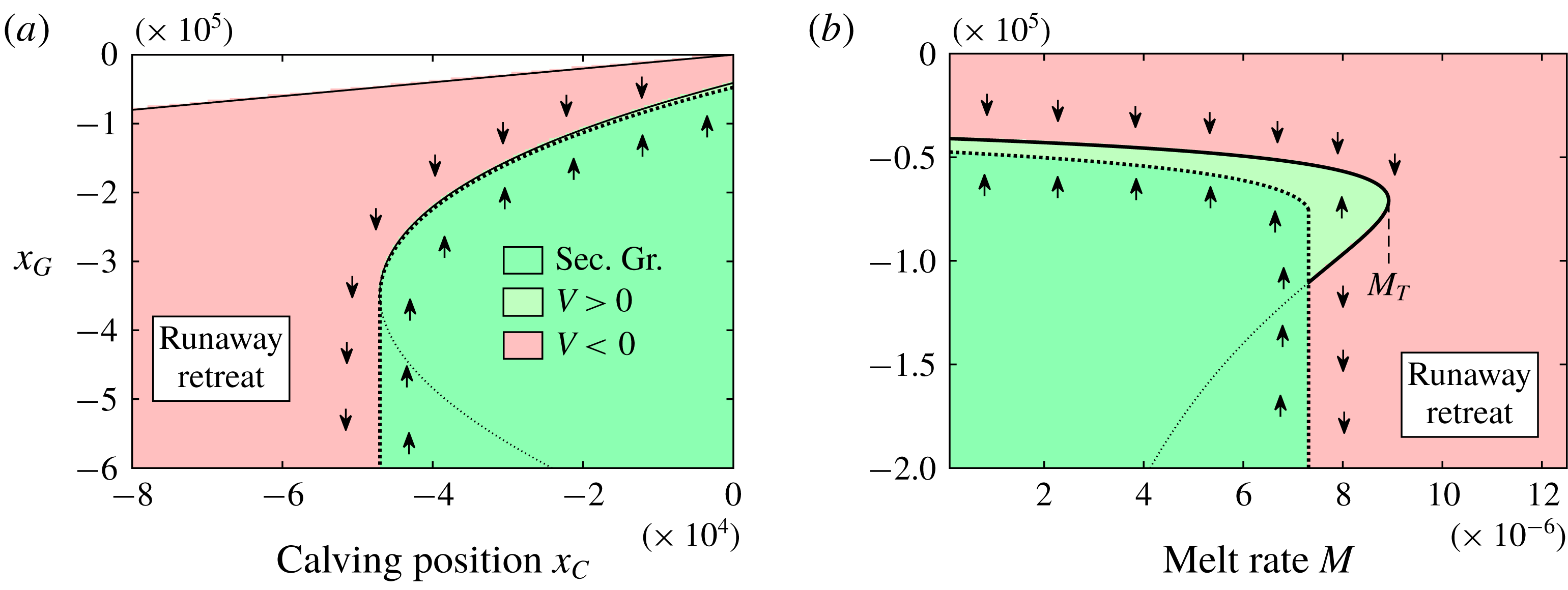
To illustrate the control of stability by the calving position
 $x_{C}$
, I show the stability diagram for
 $\unicode[STIX]{x1D6FC}=2\times 10^{-4}$
and
 $S=10^{-4}$
against a continuous variation of
 $x_{C}$
in figure 14(a). In qualitative similarity to the stability diagrams shown with respect to the lateral-drag coefficient
 $S$
(cf. figure 8), there is a stable steady-state branch above a critical value,
 $x_{C}>x_{CT}$
. The plot illustrates the retreat of the grounding line induced by retreat of the calving front, and its eventual transition to tipped retreat below the critical calving position
 $x_{C}=x_{CT}$
. Thus, if progressive retreat of the calving front occurs, there is an initial retreat of the grounding line along the stable branch before runaway grounding-line retreat triggers critically upstream of the critical position
 $x_{CT}$
interior to the retrograde slope. It is interesting to note that the conditions for tipping and recovery for this example of calving-induced tipping are almost coincident. The condition to lose a steady state is essentially the same as the condition for the ice shelf to reground. Consequently, recovery will essentially occur following parametric restoration. The hysteresis effects noted to apply for unbuttressed grounding lines (Schoof Reference Schoof2007a
) therefore practically do not occur here. It should be noted that the results here are for a prescribed calving position
 $x_{C}$
. For a thickness-dependent calving law (e.g. Schoof et al.
Reference Schoof, Davis and Popa2017),
 $x_{C}$
can be treated as an unknown and its prescription replaced by imposition of the implicit condition
 $H(x_{C})=H_{C}$
. In this case, the conditions for tipping are likely highly sensitive to the parameter
 $H_{C}$
, and this could be illustrated by a bifurcation diagram constructed for this case.
To demonstrate the destabilisation as a consequence of increased melting, I plot the stability diagram with respect to the dimensionless melt rate
 $M$
in figure 14(b), which is assumed to take a uniform value along the ice shelf for this example. The plot shows a critical melt rate
 $M_{T}$
above which a transition to tipped retreat of the grounding line occurs. Interestingly, the steady-state position of the grounding line stays relatively insensitive to the melt rate along the entire stable branch. This indicates the potential for a more abrupt transition to tipped retreat in situations where the destabilisation is induced by increasing melt rate. The critical melt rate below which secondary grounding occurs,
 $M_{\ast }$
, is also appreciably smaller than the critical value
 $M_{T}$
representing the termination of the steady-state branch. Based on a comparison between this stability diagram and that obtained for calving-induced tipping (figure 14
a), it is indicated that hysteresis is more plausible for melt-induced tipping. That is, a grounding-line retreat stimulated by melting may be relatively harder to reverse compared to a retreat triggered by calving. This difference can be attributed to the fact that melting decreases the thickness along the longitudinal interior of the ice shelf, which makes secondary grounding harder to instigate.
The examples given above indicate general features of how a grounding-line retreat is triggered on a retrograde slope upstream of a topographic maximum. As noted above, other configurations involving more specialised features could be determined by applying the analytical machinery developed here on a case by case basis. This includes the prescription of alternative calving laws, nonlinear bed topographies and a large-scale nonlinear distributed accumulation field, for example, which are readily accounted for within the analytical framework presented here. A suite of additional examples is provided in the supplementary document demonstrating the construction of the bifurcation diagrams for nonlinear bed topographies, as well as a case of a large-scale distributed accumulation field. The approach of constructing the stability diagram provides both conceptual insight into the general conditions for tipped retreat to trigger and considerable numerical efficiency for scenario exploration and sensitivity analysis.
7 Conclusions
In this paper, I have analysed the mechanisms underlying the onset of and suppression of marine ice sheet instability. A central conclusion is that the onset of instability has the characteristic of a ‘cliff edge’ with an abrupt transition from a mode of easily reversible ‘stable’ retreat into a mode of almost irreversible ‘tipped retreat’. The tipping points are identified as occurring abruptly below thresholds of parametric variation and occur at the vanishing of steady-state branches. The grounding-line positions at which these parametric thresholds are crossed can occur either midway along a retrograde slope or at a topographic maximum. A complete regime diagram moving continuously away from the unbuttressed case was constructed and provides a clear visual demonstration of how buttressed tipping points are distinct from unbuttressed tipping points. The regime diagram illustrates that for certain modes of tipping, the long-term trajectory of the ice sheet’s evolution is dependent on hysteresis (for example whether it has already tipped into instability), as applies to an unbuttressed tipping transition. For others, the long-term recovery or collapse of the ice sheet does not depend on hysteresis. That is, certain parameter values are guaranteed unconditionally to result in stabilisation or collapse without reference to the initial state of the system (for example, whether the grounding line has already tipped). This situation is found to apply if tipping is induced by a loss of ice-shelf buttressing, for which there is an abrupt switch between guaranteed stability (or recovery from a previously tipped state) and guaranteed retreat across the tipping threshold. For situations where the suppression of marine ice sheet instability is controlled by the buttressing force, the basal condition of the ice sheet plays almost no role in setting the conditions for triggering instability, differing significantly from unbuttressed tipping. The critical conditions for buttressing-controlled tipping depend primarily on the details of the ice-shelf dynamics, with the control of tipping being related to the length, lateral drag parameters, calving position and melt rate of the ice shelf.
A method of constructing bifurcation diagrams for grounding lines was developed in which steady states, the direction in which a perturbation from them will migrate, and the prediction of secondary grounding of the ice shelf, are each integrated systematically. The direction of grounding-line migration inferred from the stability diagram was confirmed using time-dependent solutions of the governing quasi-two-dimensional equations. A remarkable result is that the critical prediction of secondary grounding in steady state simply overrides the direction of grounding-line migration derived under an assumption that the buttressing force stems from lateral stresses alone, to imply unconditional advancement. There is therefore a sharp transition in the direction of grounding-line migration across a parametric threshold.
For ocean depths sufficiently low that the topography allows for an unstable grounding-line position in the unbuttressed case, the effect of lateral stresses on a positive bed slope is to cause the locally unstable steady state to move upstream. For these situations, the hysteresis effect noted previously for the unbuttressed case is possible, but becomes harder to produce. At a critical value, the unstable steady state is abruptly invalidated by secondary grounding, with the steady-state ice-shelf profile necessary to sustain the steady state predicted to penetrate the bedrock. The prediction of secondary grounding in steady state is confirmed to lead to unconditional advance of the grounding line even if the grounding line is initiated far upstream into territory where it would undergo rapid positive-feedback tipped retreat if the geometry were such as to preclude secondary grounding. By forming brief, glancing contacts with the bedrock in the vicinity of the grounding line, the ice shelf generates an additional time-averaged buttressing force that far exceeds that developed by lateral drag directly and is sufficiently powerful to suppress grounding-line retreat almost unconditionally. The possibility for hysteresis is thus sharply eliminated if the criterion for secondary grounding is satisfied.
The glancing contacts that can arise during the recovery of a retreated grounding line develop a tertiary mechanical component – intermediate to the fully grounded and floating regions – referred to as the ‘marginal-flotation regime’. This regime replaces the notion of a grounding line with a grounding area. Along this region, the thickness of the ice sheet straddles the critical thickness for flotation, with the base of the ice shelf ‘hovering’ above the bedrock with intermittent contact. The creation of this zone is caused by the thickening of the interior of the ice shelf by lateral stresses, which induces the contact, combined with a switchback mechanism in the governing conditional momentum equation creating rapid oscillations between its floating and grounded components. The existence of the marginal-flotation zone may be a hallmark of a marine ice sheet that is regenerating from a former inducement of tipped retreat, and may be an important mechanism for generating marine ice sheets during periods of glaciation.
For the case where the ocean depth is sufficiently deep that there is no steady state in the unbuttressed case, unconditional retreat of the grounding line occurs for all values of the coefficient of lateral drag below a critical tipping-point value. Above this threshold, lateral stresses produce a new branch of stable steady states. It was found that even marginally above the threshold, the ice sheet is completely secure against permanent tipping, even following a total collapse of the ice shelf. However, if the parameters in the system vary such as to produce a change to subcritical values, destabilisation of the ice sheet occurs. A natural mode of transitioning to destabilisation was demonstrated in which the grounding line retreats ‘stably’ along the stable branch in a quasi-steady manner before transitioning to ‘tipped’ retreat once the steady-state branch vanishes and the tipping point for buttressed stability is passed (at least with the assumption that the ice shelf can regrow to its former calving position). Following the transition to tipped retreat, the system will always fail to recover following a parametric restoration to former values.
However, the recovery of a tipped grounding line was determined to be possible following a recovery of parameters to values slightly more secure than the values that were necessary to trigger tipping in the first place. The restoration of the grounding line always occurs as a consequence of the ice shelf making secondary contact with the bedrock, forming an ice rise or marginal-flotation zone. Lateral stresses allow this mode of recovery to become more feasible owing to its development of a considerably thicker ice shelf. The conditions for regrounding can be almost coincident with the condition for establishing the steady state from which tipping is critically lost. This result is attributed to the property that the grounding-line position necessary to produce regrounding and the position for a buttressed steady state to form can occur very close together (Pegler Reference Pegler2018). The bifurcation diagrams show that the conditions for secondary contact are easier to attain than those necessary to instigate reversal of a tipped grounding line in the absence of any secondary grounding. The reversal of tipped grounding-line retreat is therefore dependent on and/or occurs with the formation of an ice rise or marginal-flotation zone.
A complete regime diagram for tipping and recovery of a grounding line was constructed, showing that there are two distinct criteria that can trigger a critical transition to runaway grounding-line retreat upstream of a topographic maximum. One is the buttressed threshold described above. The other is the unbuttressed threshold. The failure of both of these distinct criteria was shown to be necessary in order to induce tipping of the ice sheet upstream of a topographic maximum.
Transitions to tipped retreat induced by the retreat of a calving front or the increase in the rate of basal melting of the ice shelf were demonstrated. In the latter case, the steady-state grounding-line position was found to be relatively insensitive to melt rate before an abrupt transition to tipped retreat occurs above a critical melt rate. The tipping point resulting from an increase in melt rate produces an abrupt transition from very gradual stable retreat to sudden tipped retreat. The conditions necessary to reverse the tipped retreat driven by an increase in melting was found to be relatively harder to attain as compared to tipping induced by calving or lateral softening.
The results of this work provide a foundation for understanding the processes leading to a regional or large-scale collapse of the WAIS and paleo ice sheets. An overarching conclusion is that lateral stresses exerted on ice shelves introduces a remarkably important effect for maintaining global stability. The sustainment of mass in a marine ice sheet depends on two different controls: the setting of the grounding line, and the setting of the interior thickness upstream of the grounding line. Importantly, these properties are controlled by different physical processes and parameters. Either one of these must be the weak link in maintaining a ‘healthy’ marine ice sheet. In regards to the future of the WAIS, it can be anticipated that the control of the grounding line is likely to provide the weaker of the two links. The importance of ice shelves can be attributed to their independent contribution to the strengthening of this weakest link. The long-term stability of the WAIS is therefore likely to be contingent on the physical processes controlling the sustainment of ice shelves and their lateral contact.
Acknowledgements
I am grateful to G. Worster for comments on an early draft of this paper. I would like to thank the three anonymous referees whose comments led to significant improvement of the paper. I also thank H. Gudmundsson, I. Hewitt and B. Minchew for helpful discussions.
Supplementary material
Supplementary material is available at https://doi.org/10.1017/jfm.2018.742.