



1 Introduction
Turbulent Rayleigh–Bénard (RB) convection, which describes the convective motion of a fluid layer between two horizontal parallel plates heated from below and cooled from above, is a typical model system abstracted from many natural phenomena and industrial processes (Ahlers, Grossmann & Lohse Reference Ahlers, Grossmann and Lohse2009; Lohse & Xia Reference Lohse and Xia2010; Chillà & Schumacher Reference Chillà and Schumacher2012; Sun & Zhou Reference Sun and Zhou2014). A better knowledge of this system not only points out a convenient way of understanding complicated convection problems occurring in nature but also gives fundamental and perspective insight into some features of turbulence (Kadanoff Reference Kadanoff2001). One of the key issues that has been comprehensively investigated is to physically understand the functional form of the global heat transport, measured by the Nusselt number, defined as
 $$\begin{eqnarray}Nu=\frac{Q}{\unicode[STIX]{x1D712}\unicode[STIX]{x1D6E5}/H},\end{eqnarray}$$
as a function of the two control parameters of the system: the Rayleigh number
 $Ra$
and the Prandtl number
 $Pr$
, defined as
 $$\begin{eqnarray}Ra=\frac{\unicode[STIX]{x1D6FD}g\unicode[STIX]{x0394}H^{3}}{\unicode[STIX]{x1D708}\unicode[STIX]{x1D705}}\quad \text{and}\quad Pr=\frac{\unicode[STIX]{x1D708}}{\unicode[STIX]{x1D705}}.\end{eqnarray}$$
Here,
 $Q$
is the heat current density across the fluid layer of height
 $H$
for an imposed temperature difference
 $\unicode[STIX]{x1D6E5}$
,
 $g$
is the acceleration due to gravity and
 $\unicode[STIX]{x1D712}$
,
 $\unicode[STIX]{x1D6FD}$
,
 $\unicode[STIX]{x1D708}$
and
 $\unicode[STIX]{x1D705}$
are the thermal conductivity, thermal expansion coefficient, kinematic viscosity and thermal diffusivity of the convecting fluid, respectively. The quantities that play an important role in the heat-transport processes are the kinetic and thermal energy dissipation rates, which are respectively given by
 $$\begin{eqnarray}\unicode[STIX]{x1D700}_{u}(\boldsymbol{x},t)=\frac{1}{2}\unicode[STIX]{x1D708}\mathop{\sum }_{ij}\left[\frac{\unicode[STIX]{x2202}u_{j}(\boldsymbol{x},t)}{\unicode[STIX]{x2202}x_{i}}+\frac{\unicode[STIX]{x2202}u_{i}(\boldsymbol{x},t)}{\unicode[STIX]{x2202}x_{j}}\right]^{2}\end{eqnarray}$$
and
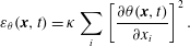 $$\begin{eqnarray}\unicode[STIX]{x1D700}_{\unicode[STIX]{x1D703}}(\boldsymbol{x},t)=\unicode[STIX]{x1D705}\mathop{\sum }_{i}\left[\frac{\unicode[STIX]{x2202}\unicode[STIX]{x1D703}(\boldsymbol{x},t)}{\unicode[STIX]{x2202}x_{i}}\right]^{2}.\end{eqnarray}$$
These two quantities denote direct dissipation of kinetic and thermal energy due to the effects of the fluid viscosity and thermal diffusivity, and can be quantified by the magnitudes of the gradients of the turbulent velocity and temperature fields,
 $\boldsymbol{u}(\boldsymbol{x},t)$
and
 $\unicode[STIX]{x1D703}(\boldsymbol{x},t)$
. As turbulent RB convection is a typical example for turbulent flows in a closed system, its local dissipation rates can be directly connected to the global heat transport through the convection cell via the two exact relations:
 $$\begin{eqnarray}\langle \unicode[STIX]{x1D700}_{u}\rangle _{V,t}=\frac{\unicode[STIX]{x1D708}^{3}}{H^{4}}(Nu-1)RaPr^{-2}\end{eqnarray}$$
and
 $$\begin{eqnarray}\langle \unicode[STIX]{x1D700}_{\unicode[STIX]{x1D703}}\rangle _{V,t}=\unicode[STIX]{x1D705}\frac{\unicode[STIX]{x1D6E5}^{2}}{H^{2}}Nu,\end{eqnarray}$$
where
 $\langle \cdot \rangle _{V,t}$
denotes an ensemble (or space–time) average. These relations form the backbone of the popular Grossmann–Lohse (GL) theory of turbulent heat transfer (Grossmann & Lohse Reference Grossmann and Lohse2000, Reference Grossmann and Lohse2004).
Due to the difficulty in the measurements of velocity or temperature gradients, the experimental studies on the dissipation rates are rather limited in the field of turbulent RB convection. The first attempt on this subject was carried out by He, Tong & Xia (Reference He, Tong and Xia2007) and He & Tong (Reference He and Tong2009), who used four identical thermistors to simultaneously measure the three components of the local temperature gradient. The time-averaged thermal energy dissipation rate was then decomposed into two contributions: one comes from the mean temperature gradient that concentrates in the thermal boundary layers (BL) and the other generated by thermal plumes that dominates in the bulk region. Using the same data set, He, Tong & Ching (Reference He, Tong and Ching2010), He, Ching & Tong (Reference He, Ching and Tong2011) further constructed a locally averaged thermal dissipation rate over a time interval
 $\unicode[STIX]{x1D70F}$
, which was found to exhibit good scaling in
 $\unicode[STIX]{x1D70F}$
with exponents being in excellent agreement with those predicted by a phenomenological intermittency model. By measuring the second-order velocity structure functions in the dissipative range, the time-averaged kinetic energy dissipation rate was indirectly obtained at the cell centre by Ni, Huang & Xia (Reference Ni, Huang and Xia2011). The
 $Ra$
dependence of the measured results was found to agree with the predictions of the GL model and it was shown that local kinetic energy dissipation rate balances local heat flux in the central region of turbulent thermal convection.
Compared with the difficulty in experiments, the direct numerical simulations (DNS) data enable the calculation of dissipation rates. The pioneering work on this subject was performed by Verzicco & Camussi (Reference Verzicco and Camussi2003) and Verzicco (Reference Verzicco2003), who analysed the statistical properties of
 $\unicode[STIX]{x1D700}_{u}$
and
 $\unicode[STIX]{x1D700}_{\unicode[STIX]{x1D703}}$
in a cylindrical cell of aspect ratio one half. Later, Shishkina & Wagner (Reference Shishkina and Wagner2006, Reference Shishkina and Wagner2008) investigated the formation and development of thermal plumes and their interaction via evaluating the thermal dissipation rates. Emran & Schumacher (Reference Emran and Schumacher2008) examined the probability density functions (PDF) of the thermal dissipation rates in a cylindrical cell. They found that, similarly to passive scalar mixing, the PDFs deviate significantly from a log-normal distribution and the PDF tails can be well fitted by a stretched exponential function. Furthermore, Kaczorowski & Wagner (Reference Kaczorowski and Wagner2009) used the PDFs of
 $\unicode[STIX]{x1D700}_{\unicode[STIX]{x1D703}}$
to distinguish the three different physical regions in a long rectangular cell via the two inflection points of the PDFs. Ng et al. (Reference Ng, Ooi, Lohse and Chung2015) calculated in vertical natural convection the dissipation contributions that come from respectively the BL and bulk regions, and their results revealed that the contributions scale as those predicted by the GL theory. Recently, Petschel et al. (Reference Petschel, Stellmach, Wilczek, Lülff and Hansen2013, Reference Petschel, Stellmach, Wilczek, Lülff and Hansen2015) put forward the idea of dissipation layers, which are based on the systematic measurements of the dissipation rates and were found to share central characteristics with classical BLs. In addition, such dissipation layers can be extended naturally to arbitrary boundary conditions.
In the paper, we provide a detailed statistical analysis of the kinetic and thermal energy dissipation rates in two-dimensional (2-D) turbulent RB convection by means of the DNS data for
 $10^{6}\leqslant Ra\leqslant 10^{10}$
and for
 $Pr=0.7$
and 5.3. Two considerations prompted us to restrict ourselves to the 2-D geometry: (i) the numerical effort required for 2-D simulations is much smaller so that a good resolution of the BLs as well as of the dissipation events at high Rayleigh/Reynolds numbers is guaranteed and systematic studies can be performed; (ii) many well-cited theories for turbulent RB systems are essentially two-dimensional, e.g. the popular GL theory (Grossmann & Lohse Reference Grossmann and Lohse2000) and the recent Whitehead–Doering theory for the ultimate regime (Whitehead & Doering Reference Whitehead and Doering2011).
The remainder of this paper is organized as follows. In § 2, we give a brief description of the governing equations and numerical model. The numerical results are presented and analysed in § 3, which is divided into four parts. Section 3.1 describes the global features of the simulations. Section 3.2 studies PDFs of
 $\unicode[STIX]{x1D700}_{u}$
and
 $\unicode[STIX]{x1D700}_{\unicode[STIX]{x1D703}}$
. In § 3.3, we compare the dissipation contributions coming from the bulk with those coming from the BL regions. The
 $Ra$
and
 $Re$
dependences of
 $\langle \unicode[STIX]{x1D700}_{u}\rangle$
and
 $\langle \unicode[STIX]{x1D700}_{\unicode[STIX]{x1D703}}\rangle$
are presented and discussed in § 3.4. Finally, we summarize our findings in § 4.
2 Numerical methods
The mathematical model and the numerical scheme have been described in detail elsewhere (Huang & Zhou Reference Huang and Zhou2013; Zhou Reference Zhou2013; Qiu, Liu & Zhou Reference Qiu, Liu and Zhou2014; Zhou et al.
Reference Zhou, Huang, Lu, Liu and Ni2016) and thus we give only their main features here. The computational domain consists of a 2-D box with uniform grids and of unit aspect ratio (i.e. ratio of the horizontal length
 $L$
to the cell height
 $H$
,
 $\unicode[STIX]{x1D6E4}=L/H=1$
). While the two vertical side walls are chosen to be adiabatic, cold and hot fixed temperatures,
 $\unicode[STIX]{x1D703}=-0.5$
and 0.5, are applied to the top and bottom plates, respectively. All the solid surfaces satisfy the no-penetration and no-slip velocity boundary conditions.
The flow is solved by the numerical integration of the 2-D time-dependent Navier–Stokes equations in vorticity–streamfunction formulation under the Boussinesq approximation. The numerical scheme is a compact fourth-order central finite-difference method (Liu, Wang & Johnston Reference Liu, Wang and Johnston2003). The equations are given by
 $$\begin{eqnarray}\displaystyle & \displaystyle \frac{\unicode[STIX]{x2202}\unicode[STIX]{x1D714}}{\unicode[STIX]{x2202}t}+(\boldsymbol{u}\boldsymbol{\cdot }\unicode[STIX]{x1D735})\unicode[STIX]{x1D714}=\unicode[STIX]{x1D708}\unicode[STIX]{x1D6FB}^{2}\unicode[STIX]{x1D714}+\frac{\unicode[STIX]{x2202}\unicode[STIX]{x1D703}}{\unicode[STIX]{x2202}x}, & \displaystyle\end{eqnarray}$$
 $$\begin{eqnarray}\displaystyle & \displaystyle \unicode[STIX]{x1D6FB}^{2}\unicode[STIX]{x1D713}=\unicode[STIX]{x1D714}, & \displaystyle\end{eqnarray}$$
 $$\begin{eqnarray}u=-\frac{\unicode[STIX]{x2202}\unicode[STIX]{x1D713}}{\unicode[STIX]{x2202}z},\quad w=\frac{\unicode[STIX]{x2202}\unicode[STIX]{x1D713}}{\unicode[STIX]{x2202}x},\end{eqnarray}$$
 $$\begin{eqnarray}\frac{\unicode[STIX]{x2202}\unicode[STIX]{x1D703}}{\unicode[STIX]{x2202}t}+(\boldsymbol{u}\boldsymbol{\cdot }\unicode[STIX]{x1D735})\unicode[STIX]{x1D703}=\unicode[STIX]{x1D705}\unicode[STIX]{x1D6FB}^{2}\unicode[STIX]{x1D703},\end{eqnarray}$$
where
 $u$
and
 $w$
are, respectively, the horizontal and vertical components of the velocity field,
 $\unicode[STIX]{x1D713}$
is the streamfunction and
 $\unicode[STIX]{x1D714}=\unicode[STIX]{x2202}w/\unicode[STIX]{x2202}x-\unicode[STIX]{x2202}u/\unicode[STIX]{x2202}z$
is the vorticity field. The equations have been made non-dimensional by using the cell height
 $H$
, the temperature difference
 $\unicode[STIX]{x1D6E5}$
and the free-fall velocity
 $U=\sqrt{\unicode[STIX]{x1D6FD}g\unicode[STIX]{x0394}H}$
, and hence the corresponding fluid viscosity
 $\unicode[STIX]{x1D708}=\sqrt{Pr/Ra}$
and thermal diffusivity
 $\unicode[STIX]{x1D705}=\sqrt{1/PrRa}$
. In our present study, the Rayleigh number was varied from
 $10^{6}$
to
 $10^{10}$
, while the Prandtl number was fixed at
 $Pr=0.7$
and 5.3, respectively corresponding to the working fluids of air (du Puits, Resagk & Thess Reference du Puits, Resagk and Thess2007) and water at
 $31^{\circ }$
(Zhou et al.
Reference Zhou, Liu, Li and Zhong2012). In table 1, we list the flow and grid parameters of the simulations.
Simulation parameters. The columns from left to right indicate the following:
 $Pr$
,
 $Ra$
, the resolution in horizontal and vertical directions
 $N_{x}\times N_{z}$
,
 $Nu$
,
 $Re=U_{rms}H/\unicode[STIX]{x1D708}$
with
 $U_{rms}=\sqrt{\langle (u^{2}+w^{2})\rangle _{V,t}}$
,
 $\langle \unicode[STIX]{x1D700}_{u}\rangle _{V,t}$
compared with that obtained from the exact relation
 $\langle \unicode[STIX]{x1D700}_{u}\rangle =\unicode[STIX]{x1D708}^{3}/H^{4}(Nu-1)RaPr^{-2}=(Nu-1)/\sqrt{RaPr}$
,
 $\langle \unicode[STIX]{x1D700}_{\unicode[STIX]{x1D703}}\rangle _{V,t}$
compared with that obtained from the exact relation
 $\langle \unicode[STIX]{x1D700}_{\unicode[STIX]{x1D703}}\rangle =\unicode[STIX]{x1D705}\unicode[STIX]{x1D6E5}^{2}/H^{2}Nu=Nu/\sqrt{RaPr}$
, the number of grid points within the thermal BL
 $N_{BL}$
, the grid spacing
 $\unicode[STIX]{x1D6E5}_{g}$
compared with the Kolmogorov scale estimated by the global criterion
 $\unicode[STIX]{x1D702}=HPr^{1/2}/[Ra(Nu-1)]^{1/4}$
,
 $\unicode[STIX]{x1D6E5}_{g}$
compared with the Batchelor scale
 $\unicode[STIX]{x1D702}_{B}=\unicode[STIX]{x1D702}Pr^{-1/2}$
(Silano, Sreenivasan & Verzicco Reference Silano, Sreenivasan and Verzicco2010), the time interval
 $\unicode[STIX]{x1D6E5}_{t}$
compared with the Kolmogorov time scale
 $\unicode[STIX]{x1D70F}_{\unicode[STIX]{x1D702}}=\sqrt{\unicode[STIX]{x1D708}/\langle \unicode[STIX]{x1D700}_{u}\rangle }=\sqrt{Pr/(Nu-1)}$
.

We briefly comment on the spatial and temporal resolutions. For the numerical study of turbulent RB convection, the mesh size must be set to achieve a full resolution of the BLs (Shishkina et al.
Reference Shishkina, Stevens, Grossmann and Lohse2010), as well as to resolve the smallest scales of the flow, these being the dissipative scales, i.e. the Kolmogorov scale
 $\unicode[STIX]{x1D702}$
and the Batchelor scale
 $\unicode[STIX]{x1D702}_{B}$
. In the present study, the number of grid points was generally chosen to be the same for the two different
 $Pr$
, except for the highest Rayleigh number
 $Ra=10^{10}$
, and was increased from
 $129\times 129$
to
 $3073\times 3073$
for
 $Ra$
increasing from
 $10^{6}$
to
 $10^{10}$
. In table 1, we list the number of grids
 $N_{BL}$
within the thermal BL and the grid spacing
 $\unicode[STIX]{x1D6E5}_{g}$
is compared with
 $\unicode[STIX]{x1D702}$
and
 $\unicode[STIX]{x1D702}_{B}$
for each simulation. It is seen that for all of our simulations the thermal BL is resolved with at least 10 grid points and the grid spacing
 $\unicode[STIX]{x1D6E5}_{g}\lesssim 0.57\unicode[STIX]{x1D702}$
and
 $\unicode[STIX]{x1D6E5}_{g}\lesssim 0.48\unicode[STIX]{x1D702}_{B}$
. Furthermore, the uniform grids adopted in the present study ensure the spatial resolution at the side walls to be the same as that close to the top and bottom plates. The viscous BLs near both the plates and side walls are resolved with at least 8 grid points at lower
 $Pr$
and with at least 16 grid points at higher
 $Pr$
, due to the increasing viscous BL thickness with increasing
 $Pr$
. To check whether the present temporal resolution resolves the smallest time scale in turbulence, we also compare the simulation time interval
 $\unicode[STIX]{x1D6E5}_{t}$
with the Kolmogorov time scale
 $\unicode[STIX]{x1D70F}_{\unicode[STIX]{x1D702}}$
in table 1. One sees that
 $\unicode[STIX]{x1D6E5}_{t}/\unicode[STIX]{x1D70F}_{\unicode[STIX]{x1D702}}<0.01$
for all runs, thus guaranteeing the adequate temporal resolution. We note that the present spatial resolutions also obey the criterion proposed by Grötzbach (Reference Grötzbach1983) and the time step
 $\unicode[STIX]{x1D6E5}_{t}$
is chosen to fulfil the Courant–Friedrichs–Lewy (CFL) conditions, i.e. the CFL number is 0.3 or less for all computations presented in this paper.
(a,b) Typical snapshots of the instantaneous temperature (colour) and velocity (arrows) fields for
 $Ra=10^{10}$
and for
 $Pr=0.7$
(a) and 5.3 (b). (c–f) The corresponding logarithmic fields of kinetic
 $\log _{10}\unicode[STIX]{x1D700}_{u}(x,z)$
(c,d) and thermal
 $\log _{10}\unicode[STIX]{x1D700}_{\unicode[STIX]{x1D703}}(x,z)$
(e,f) energy dissipation rates for
 $Pr=0.7$
(c,e) and 5.3 (d,f).

Another way to verify the grid resolution is to test whether the two global exact relations (1.5) and (1.6) hold for the simulations, as suggested by Stevens, Verzicco & Lohse (Reference Stevens, Verzicco and Lohse2010). The sixth and seventh columns of table 1 compare the directly calculated dissipation rates with those obtained from
 $Ra$
,
 $Pr$
and
 $Nu$
via the exact relations. One sees that for most of the cases the difference is less than 1 %. This guarantees the adequate resolution for small-scale turbulent structures, like thermal plumes, even in the regions very close to the horizontal plates and close to the vertical side walls.
3 Results and discussion
3.1 Global features
In figures 1(a,b), we show typical examples of the instantaneous velocity fields (arrows), overlapped with the corresponding temperature fields (colour), obtained from the simulations with
 $Ra=10^{10}$
and with
 $Pr=0.7$
and 5.3, respectively. As shown in figure 1(b), the overall flow pattern consists of a large counter-clockwise (or clockwise in some cases) rotatory motion in the bulk and several smaller secondary rolls at the four corners. This flow pattern is the same as those observed in previous studies (Sugiyama et al.
Reference Sugiyama, Calzavarini, Grossmann and Lohse2009, Reference Sugiyama, Ni, Stevens, Chan, Zhou, Xi, Sun, Grossmann, Xia and Lohse2010; Zhou et al.
Reference Zhou, Sugiyama, Stevens, Grossmann, Lohse and Xia2011; Chandra & Verma Reference Chandra and Verma2013) and is found to be stable for most of the time and for most of the runs, except for the simulation with
 $Ra=10^{10}$
and
 $Pr=0.7$
, where the corner-flow rolls are always not stable and would detach from the corners (see figure 1
a).
Figure 1(c–f) respectively displays the corresponding logarithmic fields of kinetic
 $\log _{10}\unicode[STIX]{x1D700}_{u}$
and thermal
 $\log _{10}\unicode[STIX]{x1D700}_{\unicode[STIX]{x1D703}}$
dissipation rates, where the local dissipation rate is indicated according to the colour bar. It is seen that the intense dissipations of both
 $\unicode[STIX]{x1D700}_{u}$
and
 $\unicode[STIX]{x1D700}_{\unicode[STIX]{x1D703}}$
occur nearly in the regions with higher or lower temperature, which correspond to hot or cold plumes detaching from the thermal BLs. This suggests that the rising and falling thermal plumes are associated with large amplitudes of both kinetic and thermal dissipation rates (Kerr Reference Kerr1996; Shishkina & Wagner Reference Shishkina and Wagner2007; Emran & Schumacher Reference Emran and Schumacher2008). This also suggests a strong positive correlation between the two dissipation fields. Indeed, our calculation shows that the correlation coefficient between
 $\unicode[STIX]{x1D700}_{u}$
and
 $\unicode[STIX]{x1D700}_{\unicode[STIX]{x1D703}}$
is larger than 0.4 for all the simulations, similar to the findings in 2-D Rayleigh–Taylor turbulence by Zhou & Jiang (Reference Zhou and Jiang2016).
Log–log plots of
 $Nu$
(a) and
 $Re$
(b) as functions of
 $Ra$
for
 $Pr=0.7$
(circles) and
 $5.3$
(triangles). The dashed lines are the best power-law fits to the corresponding data. The insets show the compensated plots
 $NuRa^{-0.3}$
versus
 $Ra$
and
 $ReRa^{-0.6}$
versus
 $Ra$
.

We now come to the scaling relations of the Nusselt number
 $Nu$
and the Reynolds number
 $Re$
versus the Rayleigh number
 $Ra$
. In the present study,
 $Nu$
was calculated over the whole cell and over time via the definition (Verzicco & Camussi Reference Verzicco and Camussi2003; Verzicco & Sreenivasan Reference Verzicco and Sreenivasan2008)
 $$\begin{eqnarray}Nu=1+\sqrt{PrRa}\langle w\unicode[STIX]{x1D703}\rangle _{V,t}.\end{eqnarray}$$
Due to the zero value for the velocity average over the whole cell, we here choose the root-mean-square (r.m.s.) velocity to define the Reynolds number (Sugiyama et al. Reference Sugiyama, Calzavarini, Grossmann and Lohse2009), i.e.
 $$\begin{eqnarray}Re=\frac{U_{rms}H}{\unicode[STIX]{x1D708}},\end{eqnarray}$$
where
 $U_{rms}=\sqrt{\langle (u^{2}+w^{2})\rangle _{V,t}}$
can be used as a global measure for the strength of the convection. The convergence of both
 $Nu$
and
 $Re$
has been checked by comparing the time averages over the first and the last halves of each simulation, and the resulting relative error was smaller than
 $1\,\%$
for all of our simulations.
Figure 2(a) shows a log–log plot of the measured
 $Nu$
as a function of
 $Ra$
for the two Prandtl numbers
 $Pr=0.7$
(circles) and 5.3 (triangles). The data can be well described by a power-law relation and the best fit gives
 $Nu=0.099Ra^{-0.30\pm 0.02}$
, shown as the dashed line in the figure. We note that the present scaling agrees well with the previous numerical results found also in 2-D convection cells (Johnston & Doering Reference Johnston and Doering2009; van der Poel, Stevens, Sugiyama & Lohse Reference van der Poel, Stevens, Sugiyama and Lohse2012). We further note that the exponent
 $0.30\pm 0.02$
is in general consistent with those obtained in 3-D cylindrical RB systems (Ahlers et al.
Reference Ahlers, Grossmann and Lohse2009; Chillà & Schumacher Reference Chillà and Schumacher2012). This suggests that the heat transport in both 2-D and 3-D convection might be dominated by the same physical mechanism, and thus they could be modelled in a similar way. Indeed, as we shall see in § 3.3, the results obtained in the present 2-D settings obey the GL phase diagram obtained for 3-D convection. Nevertheless, the prefactor 0.099 in the best fit relation is smaller than its counterpart for the 3-D cases where it varies between 0.12 and 0.15 (see, e.g. figure 2 of Wagner, Shishkina & Wagner (Reference Wagner, Shishkina and Wagner2012)). The possible reason is that in a closed system the convective flow would sometimes make hot (cold) plumes move downwards (upwards) and thus lead to strong count gradient/negative local heat flux (Huang & Zhou Reference Huang and Zhou2013), which impedes the overall heat transfer. This happens much more in two dimensions than in three dimensions.
Figure 2(b) displays the measured
 $Re$
as a function of
 $Ra$
in a log–log plot. Due to the decreasing viscosity
 $\unicode[STIX]{x1D708}$
, the Reynolds number for
 $Pr=0.7$
is found to be much larger than that for
 $Pr=5.3$
. The best power-law fit to the data yields
 $Re\sim Ra^{0.59\pm 0.02}$
for
 $Pr=0.7$
and
 $Re\sim Ra^{0.60\pm 0.01}$
for
 $Pr=5.3$
. The fitted scaling exponents are in excellent agreement with the exponent 0.62 found for 2-D Boussinesq RB convection by Sugiyama et al. (Reference Sugiyama, Calzavarini, Grossmann and Lohse2009), but are notably larger than those varying from 0.42 to 0.5 seen for 3-D RB flows in various convecting fluids with wide parameter range and based on the single- or multi-point measurements. (Ashkenazi & Steinberg Reference Ashkenazi and Steinberg1999; Niemela et al.
Reference Niemela, Skrbek, Sreenivasan and Donnelly2001; Qiu & Tong Reference Qiu and Tong2001; Lam et al.
Reference Lam, Shang, Zhou and Xia2002; Sun & Xia Reference Sun and Xia2005; Brown, Funfschilling & Ahlers Reference Brown, Funfschilling and Ahlers2007). The difference in
 $Re$
scaling is not captured by the GL model and implies that the convective flow in two dimensions has a stronger strength than in three dimensions. Indeed, direct comparison between 2-D and 3-D convection revealed a higher absolute value of the Reynolds number in two dimensions (van der Poel, Stevens & Lohse Reference van der Poel, Stevens and Lohse2013). The possible reason is that in the 2-D geometry almost all plumes emitted from the top and bottom thermal BLs follow the motion of the large-scale convective rolls (including the corner-flow rolls), and then drive these large-scale rolls, due to the absence of the fluid motion in the third dimension, whereas this is not the case for three dimensions (van der Poel et al.
Reference van der Poel, Stevens and Lohse2013).
3.2 Probability density functions (PDFs) of
 $\unicode[STIX]{x1D700}_{u}$
and
$\unicode[STIX]{x1D700}_{\unicode[STIX]{x1D703}}$


Next, we investigate the statistics of the kinetic
 $\unicode[STIX]{x1D700}_{u}$
and thermal
 $\unicode[STIX]{x1D700}_{\unicode[STIX]{x1D703}}$
energy dissipation rates in this section. Figures 3(a,b) show the PDFs of
 $\unicode[STIX]{x1D700}_{u}$
obtained at
 $Pr=0.7$
and 5.3, respectively. The corresponding PDFs of
 $\unicode[STIX]{x1D700}_{\unicode[STIX]{x1D703}}$
are shown in figures 4(a,b). All data have been normalized with respect to their root-mean-square (r.m.s.) values
 $(\unicode[STIX]{x1D700}_{u})_{rms}=\sqrt{\langle \unicode[STIX]{x1D700}_{u}^{2}\rangle _{V,t}}$
and
 $(\unicode[STIX]{x1D700}_{\unicode[STIX]{x1D703}})_{rms}=\sqrt{\langle \unicode[STIX]{x1D700}_{\unicode[STIX]{x1D703}}^{2}\rangle _{V,t}}$
. In the figures, two features are worthy of note. First, for both
 $\unicode[STIX]{x1D700}_{u}$
and
 $\unicode[STIX]{x1D700}_{\unicode[STIX]{x1D703}}$
, the PDF tails become more extended with increasing
 $Ra$
(and thus with increasing
 $Re$
), implying an increasing degree of small-scale intermittency possessed by the both dissipation fields. This is in spite of the fact that the intermittency effects are expected to be absent for the velocity field in 2-D turbulent convection, as shown by Celani et al. (Reference Celani, Matsumoto, Mazzino and Vergassola2002). It should be noted that the convective flow studied by Celani et al. (Reference Celani, Matsumoto, Mazzino and Vergassola2002) is forced by a mean gradient, which has different boundary conditions from the present RB setting. Whether the intermittency in the statistics of velocity fluctuations is absent also in the present system needs to be verified, which requires a detailed study on the high-order moments of velocity increments. Second, at a given Rayleigh number, the PDFs of both
 $\unicode[STIX]{x1D700}_{u}$
and
 $\unicode[STIX]{x1D700}_{\unicode[STIX]{x1D703}}$
obtained at lower Prandtl number
 $(Pr=0.7)$
have a fatter tail than those obtained at higher Prandtl number
 $(Pr=5.3)$
. The reason for this might be attributed to the increasing
 $Re$
(and thus an increasing degree of intermittency) with decreasing
 $Pr$
, as shown in figure 2(b). This is in line with the observations in 3-D cylindrical RB systems (He et al.
Reference He, Tong and Xia2007; Emran & Schumacher Reference Emran and Schumacher2008), but is different from the results observed by Schumacher & Sreenivasan (Reference Schumacher and Sreenivasan2005) for the passive scalar case, where the decreasing diffusivity with increasing
 $Pr$
causes sharper gradients of the scalar field and hence generates fatter PDF tails.
(a,b) PDFs of the kinetic energy dissipation rates,
 $\unicode[STIX]{x1D700}_{u}$
, obtained over the whole cell and normalized with respect to their r.m.s. values
 $(\unicode[STIX]{x1D700}_{u})_{rms}$
. The solid lines are the best fits of stretched exponentials, as given by (3.3), to the corresponding tails. (c,d) PDFs of
 $\log _{10}\unicode[STIX]{x1D700}_{u}$
calculated over the whole cell. Here,
 $\unicode[STIX]{x1D707}$
and
 $\unicode[STIX]{x1D70E}$
are, respectively, the mean value and standard deviation of
 $\log _{10}\unicode[STIX]{x1D700}_{u}$
. The dashed lines mark the log-normal distribution for comparison. The data are obtained at
 $Pr=0.7$
(a,c) and 5.3 (b,d).

(a,b) PDFs of the thermal energy dissipation rates,
 $\unicode[STIX]{x1D700}_{\unicode[STIX]{x1D703}}$
, obtained over the whole cell and normalized with respect to their r.m.s. values
 $(\unicode[STIX]{x1D700}_{\unicode[STIX]{x1D703}})_{rms}$
. The solid lines are the best fits of stretched exponentials, as given by (3.3), to the corresponding tails. (c,d) PDFs of
 $\log _{10}\unicode[STIX]{x1D700}_{\unicode[STIX]{x1D703}}$
calculated over the whole cell. Here,
 $\unicode[STIX]{x1D707}$
and
 $\unicode[STIX]{x1D70E}$
are, respectively, the mean value and standard deviation of
 $\log _{10}\unicode[STIX]{x1D700}_{\unicode[STIX]{x1D703}}$
. The dashed lines mark the log-normal distribution for comparison. The data are obtained at
 $Pr=0.7$
(a,c) and 5.3 (b,d).

Averaged vertical profiles of kinetic (a,b) and thermal (c,d) energy dissipation rates obtained at
 $Pr=0.7$
(a,c) and 5.3 (b,d). The insets show an enlarged portion of the profiles close to the bottom plate.

To quantitatively describe the shape of the measured PDF tails, we note that a stretched exponential function, i.e.
 $$\begin{eqnarray}p(Y)=\frac{C}{\sqrt{Y}}\exp (-mY^{\unicode[STIX]{x1D6FC}}),\end{eqnarray}$$
was derived analytically for the tails of passive scalar dissipation in the limit of large Peclet and Prandtl numbers in two dimensions and
 $\unicode[STIX]{x1D6FC}=1/3$
was found (Chertkov, Falkovich & Kolokolov Reference Chertkov, Falkovich and Kolokolov1998). This result was then extended to arbitrary space dimensions (Gamba & Kolokolov Reference Gamba and Kolokolov1999), as the behaviour (3.3) is determined by the dynamics of stretching (not of rotation) that is likely to take place in any dimension (Chertkov et al.
Reference Chertkov, Falkovich and Kolokolov1998). Here,
 $C$
,
 $m$
and
 $\unicode[STIX]{x1D6FC}$
are fitting parameters, and
 $Y=X-X_{mp}$
with
 $X=\unicode[STIX]{x1D700}_{\unicode[STIX]{x1D703}}/(\unicode[STIX]{x1D700}_{\unicode[STIX]{x1D703}})_{rms}$
and
 $X_{mp}$
being the abscissa of the most probable (mp) amplitude. In numerical studies of passive scalar in turbulence, the function (3.3) was found to well fit to the fraction of the dissipation PDF that extends from the mp amplitude to the end of the tail (Overholt & Pope Reference Overholt and Pope1996; Schumacher & Sreenivasan Reference Schumacher and Sreenivasan2005). The similar analysis was later conducted for active scalar in 3-D RB convection (Emran & Schumacher Reference Emran and Schumacher2008; Kaczorowski & Wagner Reference Kaczorowski and Wagner2009) and in 2-D Rayleigh–Taylor turbulence (Zhou & Jiang Reference Zhou and Jiang2016). Here, to follow this idea, we also adopted (3.3) to fit the PDF tails for both
 $\unicode[STIX]{x1D700}_{u}$
and
 $\unicode[STIX]{x1D700}_{\unicode[STIX]{x1D703}}$
obtained over the whole cell, and our results show that (3.3) can be indeed used to describe well the tails of the dissipation PDFs (see the solid lines in figures 3 and 4).
In some classical turbulence theories, like the refined similarity hypothesis proposed by Kolmogorov (Reference Kolmogorov1962), the dissipation fields are often assumed to have a log-normal distribution. However, the highly intermittent nature of the local dissipation generates the observed deviations from the log-normality (Ferchichi & Tavoularis Reference Ferchichi and Tavoularis2002; Schumacher & Sreenivasan Reference Schumacher and Sreenivasan2005; Emran & Schumacher Reference Emran and Schumacher2008; Kaczorowski & Wagner Reference Kaczorowski and Wagner2009). To check the deviations in our present systems, the dissipation PDFs are represented in log-normal coordinates in figures 3(c,d) and 4(c,d). In the figures, the dashed lines mark the log-normal distribution for reference. Clear departures from log-normality can be seen for both
 $\unicode[STIX]{x1D700}_{u}$
and
 $\unicode[STIX]{x1D700}_{\unicode[STIX]{x1D703}}$
. As
 $Ra$
increases, the cores of the PDFs seem to converge towards the log-normality and the right tails become fatter, while the left tails do not appear to show systematic trends with the Rayleigh number.
3.3 Spatial distribution of
$\unicode[STIX]{x1D700}_{u}$
and
$\unicode[STIX]{x1D700}_{\unicode[STIX]{x1D703}}$


Figure 5(a–d) show the vertical profiles of
 $\langle \unicode[STIX]{x1D700}_{u}\rangle _{x,t}$
and
 $\langle \unicode[STIX]{x1D700}_{\unicode[STIX]{x1D703}}\rangle _{x,t}$
, which illustrate the spatial distribution of the dissipation rates. Here,
 $\langle \cdot \rangle _{x,t}$
denotes an average over the horizontal direction and over time. The kinetic energy dissipation rate keeps nearly constant in the bulk, increases rapidly in the neighbourhood of the top and bottom plates where viscosity becomes significant, and reaches its maximum value at the solid-fluid interfaces. With decreasing
 $Ra$
, the magnitude of
 $\langle \unicode[STIX]{x1D700}_{u}\rangle _{x,t}$
enhances in the bulk, but drops in the BL, indicating that the kinetic energy is dissipated more equally over the whole cell at lower Rayleigh numbers. The thermal dissipation rate also attains its largest value near the plates. However, in the core region (
 $0.4\lesssim z\lesssim 0.6$
)
 $\langle \unicode[STIX]{x1D700}_{\unicode[STIX]{x1D703}}\rangle _{x,t}$
has almost a zero value for all data, suggesting that most thermal energy is dissipated within the thermal BLs.
To further quantify the spatial distribution, we calculate the dissipation contributions coming from the bulk region, separated from those coming from the BLs, i.e.
 $$\begin{eqnarray}\langle \unicode[STIX]{x1D700}_{u}\rangle _{V,t}=\langle \unicode[STIX]{x1D700}_{u}\rangle _{V_{BL},t}+\langle \unicode[STIX]{x1D700}_{u}\rangle _{V_{bulk},t},\end{eqnarray}$$
and
 $$\begin{eqnarray}\langle \unicode[STIX]{x1D700}_{\unicode[STIX]{x1D703}}\rangle _{V,t}=\langle \unicode[STIX]{x1D700}_{\unicode[STIX]{x1D703}}\rangle _{V_{BL},t}+\langle \unicode[STIX]{x1D700}_{\unicode[STIX]{x1D703}}\rangle _{V_{bulk},t},\end{eqnarray}$$
where
 $V_{BL}$
and
 $V_{bulk}$
denote the BL and bulk regions, respectively, and the averages
 $\langle \cdot \rangle _{V_{BL},t}$
and
 $\langle \cdot \rangle _{V_{bulk},t}$
have been multiplied by their corresponding volume percentages. Note that the splitting (3.4) and (3.5) are the central idea of the GL theory (Ahlers et al.
Reference Ahlers, Grossmann and Lohse2009). To do this splitting, the BL thickness must be first defined to separate the bulk and BL regions. There are quite a few definitions of BL thickness, based on either the mean velocity/temperature profiles or their r.m.s. profiles (Sun et al.
Reference Sun, Ren, Song and Xia2005; du Puits, Resagk & Thess Reference du Puits, Resagk and Thess2010; Zhou & Xia Reference Zhou and Xia2010, Reference Zhou and Xia2013; Scheel, Kim & White Reference Scheel, Kim and White2012; Scheel & Schumacher Reference Scheel and Schumacher2014; Ng et al.
Reference Ng, Ooi, Lohse and Chung2015; Shishkina et al.
Reference Shishkina, Horn, Wagner and Ching2015). In 2-D RB convection, however, due to the influences of the corner-flow rolls, the mean velocity profiles might sometimes lead to unphysical viscous BL thickness, as shown by Zhou et al. (Reference Zhou, Sugiyama, Stevens, Grossmann, Lohse and Xia2011). Therefore, in the present study, we define the viscous (thermal) BL thickness,
 $\unicode[STIX]{x1D6FF}_{u}^{rms}$
(
 $\unicode[STIX]{x1D6FF}_{\unicode[STIX]{x1D703}}^{rms}$
), as the distance between the wall and the position at which the r.m.s. velocity (temperature) is maximum. We find that this definition gives a thermal BL thickness,
 $\unicode[STIX]{x1D6FF}_{\unicode[STIX]{x1D703}}^{rms}$
, that is very close to the global estimation
 $H/(2Nu)$
. We further find that whereas
 $\unicode[STIX]{x1D6FF}_{u}^{rms}$
increases with increasing
 $Pr$
,
 $\unicode[STIX]{x1D6FF}_{\unicode[STIX]{x1D703}}^{rms}$
at each
 $Ra$
keeps nearly unchanged for both
 $Pr$
. The ratio between
 $\unicode[STIX]{x1D6FF}_{u}^{rms}$
and
 $\unicode[STIX]{x1D6FF}_{\unicode[STIX]{x1D703}}^{rms}$
varies around 0.85 for
 $Pr=0.7$
, but between 1.5 and 4 for
 $Pr=5.3$
. This is qualitatively consistent with the findings in 3-D cylindrical cells by Stevens, Lohse & Verzicco (Reference Stevens, Lohse and Verzicco2011).
Percentages of bulk (triangles) and BL (circles) contributions to the kinetic energy dissipation rates,
 $\unicode[STIX]{x1D700}_{u}$
, as functions of
 $Ra$
at
 $Pr=0.7$
(a) and 5.3 (b).

As no-slip velocity boundary conditions are applied to all the solid surfaces, the velocity field has BLs close to both the two horizontal conducting plates and the two vertical side walls, whose thicknesses are determined from the horizontal and vertical r.m.s. velocity profiles, respectively. On the other hand, due to the adiabatic side walls, the thermal BLs include only those coming from the two horizontal plates. This BL–bulk partition is consistent with the distinction proposed by the GL theory (see figure 2 of Ahlers et al. Reference Ahlers, Grossmann and Lohse2009) and has been adopted in previous studies (Verzicco Reference Verzicco2003; Verzicco & Camussi Reference Verzicco and Camussi2003).
The relative contributions of the bulk and BL regions to the total
 $\langle \unicode[STIX]{x1D700}_{u}\rangle _{V,t}$
and
 $\langle \unicode[STIX]{x1D700}_{\unicode[STIX]{x1D703}}\rangle _{V,t}$
are plotted as functions of
 $Ra$
in figures 6 and 7. It is seen that for our present parameter ranges both
 $\unicode[STIX]{x1D700}_{u}$
and
 $\unicode[STIX]{x1D700}_{\unicode[STIX]{x1D703}}$
are dominated by the BLs. Despite figures 5(a,b) reveal that at lower Rayleigh numbers the kinetic energy is dissipated more equally over the whole cell, the contribution to
 $\unicode[STIX]{x1D700}_{u}$
from the BL regions is still dominant as the BL thicknesses (and thus the volume fraction occupied by the BLs) increases with decreasing
 $Ra$
. According to these results, the present series of simulations at
 $Pr=0.7$
and 5.3 can be classified as
 $I_{l}$
and
 $I_{u}$
regimes in the GL theory, respectively. Indeed, when placing the
 $Ra$
and
 $Pr$
values of the present simulations into the phase diagram of the GL theory (see figure 2 of Grossmann & Lohse Reference Grossmann and Lohse2000), we observe reasonable agreement. Nevertheless, it should be noted that the GL phase diagram (Grossmann & Lohse Reference Grossmann and Lohse2000) is obtained for 3-D convection, while the present simulations are performed in two dimensions. Previous studies on the comparison between 2-D and 3-D RB convection (van der Poel et al.
Reference van der Poel, Stevens and Lohse2013) have revealed that the
 $Nu$
–
 $Ra$
scaling for 2-D and 3-D cases is very similar at higher
 $Pr$
, differing only by a constant factor, while the difference is large at lower
 $Pr$
, due to the strong roll state dependence of
 $Nu$
in 2-D convection.
Percentages of bulk (triangles) and BL (circles) contributions to the thermal energy dissipation rates,
 $\unicode[STIX]{x1D700}_{\unicode[STIX]{x1D703}}$
, as functions of
 $Ra$
at
 $Pr=0.7$
(a) and 5.3 (b).

As the BL–bulk partition ignores the effects of thermal plumes which should be included in the BL estimates, Grossmann & Lohse (Reference Grossmann and Lohse2004) suggested to use the labels pl (plume) and bg (background) for the two parts of the thermal energy dissipation rates, i.e.
 $$\begin{eqnarray}\langle \unicode[STIX]{x1D700}_{\unicode[STIX]{x1D703}}\rangle _{V,t}=\langle \unicode[STIX]{x1D700}_{\unicode[STIX]{x1D703}}\rangle _{V_{pl},t}+\langle \unicode[STIX]{x1D700}_{\unicode[STIX]{x1D703}}\rangle _{V_{bg},t}.\end{eqnarray}$$
Here,
 $\langle \unicode[STIX]{x1D700}_{\unicode[STIX]{x1D703}}\rangle _{V_{pl},t}$
indicates the contributions from the plumes together with the BL and
 $\langle \unicode[STIX]{x1D700}_{\unicode[STIX]{x1D703}}\rangle _{V_{bg},t}$
signals those from the background. This pl–bg partition has been adopted in some previous numerical studies to investigate the distribution of
 $\unicode[STIX]{x1D700}_{\unicode[STIX]{x1D703}}$
in 3-D cylindrical cells (Shishkina & Wagner Reference Shishkina and Wagner2006; Emran & Schumacher Reference Emran and Schumacher2012). Next, we also consider the pl–bg partition. To detect thermal plumes, we follow the approach of Huang et al. (Reference Huang, Kaczorowski, Ni and Xia2013) and van der Poel, Verzicco, Grossmann & Lohse (Reference van der Poel, Verzicco, Grossmann and Lohse2015). A thermal plume in the bulk is defined as a region where
 $$\begin{eqnarray}|\unicode[STIX]{x1D703}(x,z,t)-\langle \unicode[STIX]{x1D703}\rangle _{x,t}|>c\unicode[STIX]{x1D703}_{rms}\quad \text{and}\quad \sqrt{PrRa}|w(x,z,t)\unicode[STIX]{x1D703}(x,z,t)|>cNu.\end{eqnarray}$$
Here, we consider the absolute value of the local convective heat flux,
 $|w(x,z,t)\unicode[STIX]{x1D703}(x,z,t)|$
, because thermal plumes may sometimes generate negative local heat transport, which happens much more in two dimensions than in three dimensions, as revealed by Huang & Zhou (Reference Huang and Zhou2013). The empirical constant
 $c$
is chosen to be 1.2, which is the same as that of van der Poel et al. (Reference van der Poel, Verzicco, Grossmann and Lohse2015) but larger than the value of 0.8 chosen by Huang et al. (Reference Huang, Kaczorowski, Ni and Xia2013). In a previous work in 3-D convection, Emran & Schumacher (Reference Emran and Schumacher2012) identified thermal plumes by using a similar threshold that is based only on
 $w\unicode[STIX]{x1D703}$
and they found that the increase of the threshold by two orders of magnitude causes slight variations in the
 $Ra$
scaling. In the present work, we also find that the
 $Re$
scalings of
 $\langle \unicode[STIX]{x1D700}_{\unicode[STIX]{x1D703}}\rangle _{V_{pl},t}$
and
 $\langle \unicode[STIX]{x1D700}_{\unicode[STIX]{x1D703}}\rangle _{V_{bg},t}$
do not depend apparently on the value of threshold
 $c$
. Figure 8(b) depicts the
 $V_{pl}$
regions (in black) by applying the criterion (3.7a,b
) to the instantaneous temperature snapshot shown in figure 8(a).
(a) A snapshot of the instantaneous temperature (colour) and velocity (arrows) fields for
 $Ra=10^{10}$
and
 $Pr=5.3$
. (b) The plume regions for the same snapshot are marked in black, otherwise white.

Percentages of plume (triangles) and background (circles) contributions to the thermal energy dissipation rates,
 $\unicode[STIX]{x1D700}_{\unicode[STIX]{x1D703}}$
, as functions of
 $Ra$
at
 $Pr=0.7$
(a) and 5.3 (b).

Figures 9(a,b) shows the relative contributions from
 $V_{pl}$
and
 $V_{bg}$
to the total
 $\langle \unicode[STIX]{x1D700}_{\unicode[STIX]{x1D703}}\rangle _{V,t}$
, as functions of
 $Ra$
. Clearly,
 $\unicode[STIX]{x1D700}_{\unicode[STIX]{x1D703}}$
is plume dominated for the present parameter ranges. When varying the value of threshold
 $c$
, a systematic trend can be observed for both contributions. The smaller the threshold
 $c$
, the more the
 $V_{pl}$
contribution data are shifted upwards and those from
 $V_{bg}$
downwards. Moreover, when the threshold
 $c$
becomes large enough, the
 $V_{pl}$
region will become negligibly small and then the pl–bg partition will be the same as the BL–bulk partition.
3.4
$Ra$
and
$Re$
dependence


The
 $Ra$
dependence of
 $\langle \unicode[STIX]{x1D700}_{u}\rangle _{V,t}$
(a) and
 $\langle \unicode[STIX]{x1D700}_{\unicode[STIX]{x1D703}}\rangle _{V,t}$
(b) calculated at
 $Pr=0.7$
(circles) and 5.3 (triangles). The solid lines represent the best power-law fits to the corresponding data.

Finally, we consider the
 $Ra$
and
 $Re$
dependence of the dissipation rates. Figure 10(a,b) show the total dissipation rates,
 $\langle \unicode[STIX]{x1D700}_{u}\rangle _{V,t}$
and
 $\langle \unicode[STIX]{x1D700}_{\unicode[STIX]{x1D703}}\rangle _{V,t}$
, as functions of
 $Ra$
in log–log plots. The solid lines in the figure represent the best power-law fits to the corresponding data, which yield
 $$\begin{eqnarray}\langle \unicode[STIX]{x1D700}_{u}\rangle _{V,t}=0.077Ra^{-0.18\pm 0.02}\quad \text{and}\quad \langle \unicode[STIX]{x1D700}_{\unicode[STIX]{x1D703}}\rangle _{V,t}=0.10Ra^{-0.19\pm 0.02}\quad \text{for }Pr=0.7,\end{eqnarray}$$
 $$\begin{eqnarray}\langle \unicode[STIX]{x1D700}_{u}\rangle _{V,t}=0.036Ra^{-0.19\pm 0.01}\quad \text{and}\quad \langle \unicode[STIX]{x1D700}_{\unicode[STIX]{x1D703}}\rangle _{V,t}=0.050Ra^{-0.20\pm 0.01}\quad \text{for }Pr=5.3.\end{eqnarray}$$
One sees that
 $\langle \unicode[STIX]{x1D700}_{u}\rangle _{V,t}$
and
 $\langle \unicode[STIX]{x1D700}_{\unicode[STIX]{x1D703}}\rangle _{V,t}$
have similar scaling behaviours with
 $Ra$
but their magnitudes vary with
 $Pr$
.
To understand these scaling behaviours, we note that figure 2(a) has shown that
 $Nu\sim Ra^{0.3}$
. Plug it into the two global exact relations (1.5) and (1.6), we have
 $$\begin{eqnarray}\langle \unicode[STIX]{x1D700}_{u}\rangle _{V,t}=(Nu-1)/\sqrt{RaPr}\sim Ra^{-0.2}\quad \text{and}\quad \langle \unicode[STIX]{x1D700}_{\unicode[STIX]{x1D703}}\rangle _{V,t}=Nu/\sqrt{RaPr}\sim Ra^{-0.2}.\end{eqnarray}$$
Comparing (3.10a,b
) to our measured scalings (3.8a,b
) and (3.9a,b
) in figure 10, one observes very good agreement within numerical uncertainty, again verifying that the global exact relations for
 $\langle \unicode[STIX]{x1D700}_{u}\rangle _{V,t}$
and
 $\langle \unicode[STIX]{x1D700}_{\unicode[STIX]{x1D703}}\rangle _{V,t}$
are satisfied for our present simulations.
(a,b) The
 $Re$
dependence of the normalized dissipation in the bulk and BL regions for
 $\langle \unicode[STIX]{x1D700}_{u}\rangle /(\unicode[STIX]{x1D708}^{3}/H^{4})$
(a) and
 $\langle \unicode[STIX]{x1D700}_{\unicode[STIX]{x1D703}}\rangle /[\unicode[STIX]{x1D705}(\unicode[STIX]{x1D6E5}/H)^{2}]$
(b) obtained at
 $Pr=0.7$
and 5.3. For reference, the solid and dashed lines mark the GL predictions (3.11)–(3.14), respectively, for the BL and bulk contributions. (c) The
 $Re$
dependence of the normalized thermal energy dissipation rates in the plume and background regions. For reference, the solid and dashed lines mark the GL predictions (3.15)–(3.16), respectively, for the plume and background contributions.

The essence of the GL theory (Grossmann & Lohse Reference Grossmann and Lohse2000) is the splitting of the total dissipation rates into the contributions from the bulk and BL regions, i.e. the relations (3.4) and (3.5). By assuming that there exist a large-scale mean flow (associated with a Reynolds number
 $Re$
) in the system and that the BLs are characterized by a single effective thickness, the four contributions to the dissipation can be estimated as follows:
 $$\begin{eqnarray}\displaystyle & \displaystyle \langle \unicode[STIX]{x1D700}_{u}\rangle _{V_{BL},t}\sim \frac{\unicode[STIX]{x1D708}^{3}}{H^{4}}Re^{5/2}, & \displaystyle\end{eqnarray}$$
 $$\begin{eqnarray}\displaystyle & \displaystyle \langle \unicode[STIX]{x1D700}_{u}\rangle _{V_{bulk},t}\sim \frac{\unicode[STIX]{x1D708}^{3}}{H^{4}}Re^{3}, & \displaystyle\end{eqnarray}$$
 $$\begin{eqnarray}\displaystyle & \displaystyle \langle \unicode[STIX]{x1D700}_{\unicode[STIX]{x1D703}}\rangle _{V_{BL},t}\sim \unicode[STIX]{x1D705}\frac{\unicode[STIX]{x1D6E5}^{2}}{H^{2}}Re^{1/2}g(Pr), & \displaystyle\end{eqnarray}$$
 $$\begin{eqnarray}\displaystyle & \displaystyle \langle \unicode[STIX]{x1D700}_{\unicode[STIX]{x1D703}}\rangle _{V_{bulk},t}\sim \unicode[STIX]{x1D705}\frac{\unicode[STIX]{x1D6E5}^{2}}{H^{2}}PrRe, & \displaystyle\end{eqnarray}$$
where
 $g(Pr)$
is a function of
 $Pr$
. When the plume effects are included in the BL estimates, we have
 $$\begin{eqnarray}\displaystyle & \displaystyle \langle \unicode[STIX]{x1D700}_{\unicode[STIX]{x1D703}}\rangle _{V_{pl},t}\sim \unicode[STIX]{x1D705}\frac{\unicode[STIX]{x1D6E5}^{2}}{H^{2}}Re^{1/2}Pr^{1/2}f^{1/2}, & \displaystyle\end{eqnarray}$$
 $$\begin{eqnarray}\displaystyle & \displaystyle \langle \unicode[STIX]{x1D700}_{\unicode[STIX]{x1D703}}\rangle _{V_{bg},t}\sim \unicode[STIX]{x1D705}\frac{\unicode[STIX]{x1D6E5}^{2}}{H^{2}}RePrf, & \displaystyle\end{eqnarray}$$
where,
 $f$
is a shedding frequency that has no systematic dependence on Reynolds number. To test these scalings, we examine the
 $Re$
dependence of the normalized dissipations in figure 11. Figure 11(a,b) shows the results from the BL–bulk partition. It is seen that both the BL and bulk contributions exhibit parallel trends as
 $Re$
increases. This is consistent with the observations in figures 6 and 7, which show that the ratio of the BL-to-bulk contributions for both
 $\langle \unicode[STIX]{x1D700}_{u}\rangle$
and
 $\langle \unicode[STIX]{x1D700}_{\unicode[STIX]{x1D703}}\rangle$
appears to be constant. Figure 11(c) shows the results from the pl–bg partition for
 $\unicode[STIX]{x1D700}_{\unicode[STIX]{x1D703}}$
. Similar to the BL–bulk partition, the contributions from
 $V_{pl}$
and
 $V_{bg}$
also exhibit roughly parallel trends with increasing
 $Re$
. We further find that these trends and their
 $Re$
scaling do not change apparently with the value of threshold
 $c$
.
In addition, while the BL/plume contributions,
 $\langle \unicode[STIX]{x1D700}_{u}\rangle _{V_{BL},t}$
,
 $\langle \unicode[STIX]{x1D700}_{\unicode[STIX]{x1D703}}\rangle _{V_{BL},t}$
, and
 $\langle \unicode[STIX]{x1D700}_{\unicode[STIX]{x1D703}}\rangle _{V_{pl},t}$
, follow well the GL predictions (3.11), (3.13), and (3.15) (the solid lines in figure 11), the bulk/background contributions,
 $\langle \unicode[STIX]{x1D700}_{u}\rangle _{V_{bulk},t}$
,
 $\langle \unicode[STIX]{x1D700}_{\unicode[STIX]{x1D703}}\rangle _{V_{bulk},t}$
, and
 $\langle \unicode[STIX]{x1D700}_{\unicode[STIX]{x1D703}}\rangle _{V_{bg},t}$
deviate obviously from the predicted
 $Re$
scalings (3.12), (3.14) and (3.16) (the dashed lines in figure 11). Similar deviations for the bulk contributions have already been reported in homogeneous convection (Calzavarini et al.
Reference Calzavarini, Lohse, Toschi and Tripiccione2005), turbulent RB convection in spherical shells (Gastine, Wicht & Aurnou Reference Gastine, Wicht and Aurnou2015) and vertical natural convection (Ng et al.
Reference Ng, Ooi, Lohse and Chung2015). In the present study, the reason for the deviation of
 $\langle \unicode[STIX]{x1D700}_{u}\rangle _{V_{bulk},t}$
from (3.12) is that the GL scaling (3.12) for the bulk contributions is based on the Kolmogorov’s picture in which the kinetic energy cascades from large to small scales. This assumption, however, does not hold in 2-D RB convection, where an inverse cascade of kinetic energy from small to large scales is theoretically expected (Celani et al.
Reference Celani, Matsumoto, Mazzino and Vergassola2002). Indeed, the calculation of the third-order structure function of longitudinal velocity increments,
 $S_{3}(r)=\langle (w(r+z)-w(z))^{3}\rangle _{V,t}$
, shows that
 $S_{3}(r)$
is positive over all scales studied (not shown here), signalling the reversal of the kinetic energy cascade in the present 2-D RB setting. A detailed study on this issue is out of the scope of the present work.
4 Conclusion
In this paper, we present an analysis of the statistical properties of the kinetic and thermal energy dissipation rates in 2-D turbulent RB convection, by means of high-resolution DNS, with
 $Pr$
fixed at 0.7 and 5.3 and
 $Ra$
varying from
 $10^{6}$
to
 $10^{10}$
. Major findings are summarized as follows:
-
(i) The global heat transport and momentum scaling exponents are examined, which yields
$Nu\sim Ra^{0.30\pm 0.02}$
and
$Re\sim Ra^{0.60\pm 0.02}$
for both
$Pr$
. When comparing with previous numerical and experimental results obtained in the 3-D cases,
$Nu(Ra)$
is found to have a similar scaling exponent with smaller amplitudes, suggesting that the heat transport in both 2-D and 3-D convection might be dominated by the same physical mechanism and thus could be modelled in a similar way. Whereas the exponent of
$Re(Ra)$
is notably larger than its 3-D counterpart, implying a stronger strength of the convective flow in two dimensions than in three dimensions. -
(ii) Similar to the 3-D situations, the PDFs of both
$\unicode[STIX]{x1D700}_{u}$
and
$\unicode[STIX]{x1D700}_{\unicode[STIX]{x1D703}}$
in 2-D RB convection are found to be always non-log-normal, but their tails can be well fitted by a stretched exponential function. These tails become more extended with increasing
$Ra$
or decreasing
$Pr$
, which displays an increasing degree of small-scale intermittency with increasing
$Re$
. This is in spite of that intermittency is expected to be absent for velocity in 2-D turbulent convection (Celani et al.
Reference Celani, Matsumoto, Mazzino and Vergassola2002). The ensemble averages of both dissipation rates scale as
$Ra^{-0.18\sim -0.20}$
. This scaling exponent agrees well with those estimated from the two global exact relations (1.5) and (1.6). -
(iii) When considering the dissipation contributions that come from the bulk and BL regions, we find that
$\langle \unicode[STIX]{x1D700}_{u}\rangle _{V,t}$
and
$\langle \unicode[STIX]{x1D700}_{\unicode[STIX]{x1D703}}\rangle _{V,t}$
are both dominated by the BLs. This corresponds to regimes
$I_{l}$
and
$I_{u}$
in the GL theory (Grossmann & Lohse Reference Grossmann and Lohse2000) for our present simulations of
$Pr=0.7$
and 5.3 respectively. To include the effects of thermal plumes, the pl–bg partition is also considered and
$\langle \unicode[STIX]{x1D700}_{\unicode[STIX]{x1D703}}\rangle _{V,t}$
is found to be plume dominated. Further analysis reveals that the BL/pl contributions scale as those predicted by the GL theory, while the deviations from the GL predictions are observed for the bulk/bg contributions.


Acknowledgements
This work was supported by Natural Science Foundation of China under grant nos 11672156, 11572185, and 11332006, Shanghai Shuguang Project under grant no. 13SG40 and Program for New Century Excellent Talents in University under grant no. NCET-13. Q.Z. wishes to acknowledge support given to him from the organization department of the CPC central committee through the National Program for Support of Top-notch Young Professionals.



