1 Introduction
Wetlands, generally populated by various aquatic plants, are among the most significant ecosystems on Earth (Costanza et al. Reference Costanza, d’Arge, de Groot, Farber, Grasso, Hannon, Limburg, Naeem, O’Neill, Paruelo, Raskin, Sutton and van den Belt1997). Vast numbers of motile micro-organisms are found in wetlands, and many important ecological phenomena, such as consumption of nutrients, predation by larger organisms, harmful algal blooms (Smayda Reference Smayda1997) etc., occur as such micro-organisms interact with the vegetation. Understanding the distribution of swimming micro-organisms in shallow water containing vegetation, and possibly experiencing a slow horizontal flow (e.g. in tidal marshland), will make an important contribution to understanding the ecology of the whole biological system. The main long-term goal of our work is to be able to predict the effect of cell motility on the distribution of algal cells in the complex geometry of aquatic vegetation. This will require combining methods to compute both the flow field and the distribution of cells within it, to be compared with the distribution of passive scalars.
The type of vegetation to be considered here is so-called ‘emergent vegetation’, in which most of the leafy part of the plants is exposed to the air above the water, and is supported by less leafy stalks beneath the surface (Cronk & Fennessy (Reference Cronk and Fennessy2001), Nepf (Reference Nepf2012) and references therein). A good example is the salt-water cordgrass, Spartina alterniflora, which is native to and forms a dominant part of many coastal salt marshes on the Atlantic coast of the Americas. In the interior of a marsh there can be 200–300 stems per
 $\text{m}^{2}$
(Leonard & Luther Reference Leonard and Luther1995), indicating a mean spacing
 $l_{0}$
of 6–7 cm; the stem diameter
 $d$
is 0.10–0.25 cm (Lightbody & Nepf Reference Lightbody and Nepf2006). The height of these plants can be as much as 2–3 m, with smooth stems and culms below the water surface, except possibly at high tide. In the observations of Lightbody & Nepf (Reference Lightbody and Nepf2006) the mean water velocity ranged from zero (at low or high tide) to
 $24~\text{cm}~\text{s}^{-1}$
. Thus the Reynolds number based on stem diameter ranged from zero to 600.
In general the vegetation is flexible, but an obvious simple model of emergent vegetation is an array of rigid vertical circular cylinders in a quasi-steady, horizontal shear flow driven by a pressure gradient
 $\unicode[STIX]{x1D70C}gS$
, where
 $\unicode[STIX]{x1D70C}$
is the fluid density,
 $g$
is the gravitational acceleration and
 $S$
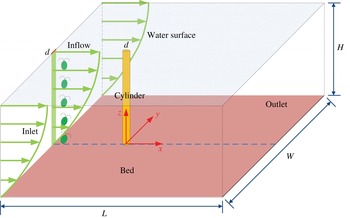
is the slope of the free surface. As a first step towards analysing the behaviour of swimming micro-organisms in such an array, this paper will be concerned with flow past a single rigid vertical cylinder that extends from a flat horizontal bed and penetrates the free surface of the fluid. Upstream of the cylinder the flow will be taken to be a unidirectional shear flow containing micro-organisms (see figure 1). For the non-uniform flow field to have a significant effect on the cell distribution, the latter must also be non-uniform, so in this paper we take the upstream cell distribution to have a particular form: cells are confined to a vertical strip of fluid, with the same width as the cylinder. This is obviously unrealistic, but any other choice would be equally so. We will be able to see the effect of the flow on horizontal mixing and, since the cell swimming introduces vertical inhomogeneity, on vertical variations as well.
Sketch of a horizontal shear flow containing a vertical strip of micro-organisms past a vertical circular cylinder.

The type of micro-organisms to be considered are motile algae, such as Chlamy domonas or Dunaliella, that normally swim upwards on average, in still fluid, because they are bottom heavy. When the fluid is flowing with non-zero vorticity, however, the cells experience a viscous torque which, when balanced against the gravitational torque induced by their bottom heaviness, causes them to swim in a non-vertical direction (or, if the horizontal vorticity exceeds a critical value, to tumble unsteadily). This process is termed gyrotaxis (Kessler Reference Kessler1985, Reference Kessler1986). Although there have been extensive investigations of the transport of passive particles in flows associated with vegetation (Lightbody & Nepf Reference Lightbody and Nepf2006; Tanino & Nepf Reference Tanino and Nepf2008; Chen, Zeng & Wu Reference Chen, Zeng and Wu2010; Nepf Reference Nepf2012; Zeng et al. Reference Zeng, Zhao, Chen, Ji, Wu and Feng2014), the characteristics and mechanisms of active micro-organisms in such flows remain unclear, due to the complexity of both swimming behaviour and flow patterns.
Swimming of gyrotactic micro-organisms strongly depends on the shear in the ambient flow. Gyrotaxis was first observed in suspensions of C. nivalis placed in a vertical pipe flow, where focussing towards the axis or the pipe wall occurred in downward or upward flow, respectively (Kessler Reference Kessler1985), unless the shear in the ambient flow was too strong to be compensated by the gravitational torque, when tumbling cells have an approximately horizontal mean swimming velocity (Bees, Hill & Pedley Reference Bees, Hill and Pedley1998). In horizontal shear flow this can lead to gyrotactic trapping (Durham & Stocker Reference Durham and Stocker2012). A general analysis of the orientation of spheroidal micro-organisms in a linear flow was performed by Pedley & Kessler (Reference Pedley and Kessler1987); the conclusions of Kessler (Reference Kessler1985, Reference Kessler1986) for spherical cells were confirmed as a special case of the predicted stable equilibrium in a weak shear flow.
There exist two types of model to describe the distribution of gyrotactic micro-organisms in general ambient flows: individual-based models in which cell trajectories are tracked from, usually, random initial conditions, and continuum models based on cell conservation. Individual models have been applied to investigate various phenomena associated with gyrotaxis, including bioconvection (Hopkins & Fauci Reference Hopkins and Fauci2002), the formation of thin phytoplankton layers in the ocean (Durham, Kessler & Stocker Reference Durham, Kessler and Stocker2009), microscale patches (Durham et al. Reference Durham, Climent, Barry, Lillo, Cencini, Boffetta and Stocker2013), accumulation caused by turbulent acceleration (De Lillo et al. Reference De Lillo, Cencini, Durham, Barry, Stocker, Climent and Boffetta2014), dispersion in two- and three-dimensional fields (Thorn & Bearon Reference Thorn and Bearon2010; Croze et al. Reference Croze, Sardina, Ahmed, Bees and Brandt2013), etc. In these models, the concentration distribution of cells is determined by counting cells in small volume elements, the resolution of which is limited by the overall number of cells in the computational domain. On the other hand, a continuum model was proposed by Pedley & Kessler (Reference Pedley and Kessler1990, Reference Pedley and Kessler1992) to describe hydrodynamic phenomena in dilute suspensions of gyrotactic micro-organisms, in which the interactions between the ambient flow and the micro-organisms were taken into account. Pedley & Kessler (Reference Pedley and Kessler1990) evaluated the mean swimming velocity and the random cell swimming, represented by a translational diffusivity tensor, as functionals of the probability density function for swimming direction, which is assumed to satisfy a quasi-steady Fokker–Planck equation. The model has been applied extensively to analyse bioconvection of gyrotactic micro-organisms, driven by the density difference between the cells and water, and occurring if the cell concentration is sufficiently large (Bees & Hill Reference Bees and Hill1998; Hill & Pedley Reference Hill and Pedley2005; Ghorai & Hill Reference Ghorai and Hill2007; Pedley Reference Pedley2010; Williams & Bees Reference Williams and Bees2011; Hwang & Pedley Reference Hwang and Pedley2014a ,Reference Hwang and Pedley b ). A comparison of an individual-based model and the population-level model for linear flows (in particular unidirectional flows) shows that the two types of model are generally in good agreement over much of parameter space, but with some significant exceptions (Bearon, Hazel & Thorn Reference Bearon, Hazel and Thorn2011). These models are currently valid only for dilute suspensions.
A key challenge for the future is how to develop a population-level model, such as a mixture theory (Lega & Passot Reference Lega and Passot2003; Wolgemuth Reference Wolgemuth2008), that can incorporate both steric and hydrodynamic interactions between swimmers in non-dilute suspensions. A promising model for rod-like micro-organisms, such as bacteria, was presented by Ezhilan, Shelley & Saintillan (Reference Ezhilan, Shelley and Saintillan2013), on the assumption that at high concentrations steric interactions between cells would be more important than hydrodynamic ones; this assumption was based on the observation that bacteria tend to align with their neighbours when very close together. The steric interactions can be modelled as an effective torque which may be included in the Fokker–Planck equation for the orientation distribution. However, in the case of approximately spherical cells it may not be possible to separate steric effects from near-field hydrodynamics. Individual-based simulations exist for simple spherical models of swimmers (e.g. Ishikawa, Simmonds & Pedley Reference Ishikawa, Simmonds and Pedley2006, Ishikawa, Pedley & Yamaguchi Reference Ishikawa, Pedley and Yamaguchi2007, Ishikawa, Locsei & Pedley Reference Ishikawa, Locsei and Pedley2008), but cannot be used for large populations because of the immense computational requirements.
As stated above, we here investigate a very simple proxy for flow through emergent vegetation: horizontal shear flow past a single vertical cylinder, and how the swimming of the micro-organisms affects the distribution of cells in that flow. We will consider first the flow field, at moderate Reynolds numbers (
 $O(100)$
), and then the effect of gyrotaxis on the cell distribution.
Flow past a circular cylinder with spanwise shear is a classical problem in fluid mechanics and has been investigated extensively (Griffin Reference Griffin1985; Williamson Reference Williamson1996; Williamson & Govardhan Reference Williamson and Govardhan2004), and there has been much research aimed at understanding the effects of Reynolds number, length-to-diameter ratio (Mukhopadhyay, Venugopal & Vanka Reference Mukhopadhyay, Venugopal and Vanka2002), end conditions (Woo, Cermak & Peterka Reference Woo, Cermak and Peterka1989; Mukhopadhyay, Venugopal & Vanka Reference Mukhopadhyay, Venugopal and Vanka1999), stiffness (Bourguet, Karniadakis & Triantafyllou Reference Bourguet, Karniadakis and Triantafyllou2011) and oscillation (Stansby Reference Stansby1976) on vortex shedding. The most striking feature in the flow is the appearance of spanwise zones, in each of which the vortex-shedding frequency is constant. This can be attributed to coupling between advection and diffusion of momentum in the spanwise direction (Mukhopadhyay et al. Reference Mukhopadhyay, Venugopal and Vanka1999). Moreover, the vortex-shedding frequency in a zone was found to be lower than would have been seen in a uniform flow with a velocity equal to the average oncoming velocity for that zone, due to near wake effects (Mukhopadhyay et al. Reference Mukhopadhyay, Venugopal and Vanka2002). Kappler et al. (Reference Kappler, Rodi, Szepessy and Badran2005) have shown that a large aspect ratio tends to result in a scattering of the size and location of zones. End effects appear in limited regions near the ends; for example, Maull & Young (Reference Maull and Young1973) reported that the effect of the ends of bluff bodies could extend inwards about 8 diameters along the spanwise direction. Mukhopadhyay et al. (Reference Mukhopadhyay, Venugopal and Vanka1999) found that the end conditions could change the range of observed Strouhal numbers. Another feature is that vertical secondary flow exists along the whole cylinder, which can be attributed to the spanwise pressure variation on the leading side and in the lee of the cylinder due to the spanwise variation of the oncoming velocity (Woo et al. Reference Woo, Cermak and Peterka1989).
This paper is organised as follows. In § 2.1, we formulate the problem, first for the flow field and then for the transport of gyrotactic micro-organisms in the flow, the relevant equations being simplified after analysis of the time scales of flow variation, cell reorientation and cell rotary diffusion. In § 2.2, we develop and test a numerical platform to solve this problem, including a computational fluid dynamics (CFD) code for the flow field, a code to solve the Fokker–Planck equation based on the finite volume method, and a code to compute the three-dimensional concentration distribution of gyrotactic micro-organisms, using OpenFOAM (www.openfoam.org). In § 2.3, the computational domain, boundary and initial conditions and mesh are described. In § 3.1, we use the results for the three-dimensional flow field to describe the characteristics of the velocity and vorticity fields; in § 3.2 we calculate the mean swimming velocity and translational diffusivity, as functions of all three vorticity components, and place the results in a database. We interpolate from this database to obtain the corresponding quantities at the relevant mesh points in order to solve the cell conservation equation for the three-dimensional distribution of both gyrotactic micro-organisms and passive particles. It is the difference between these two distributions that reveals the effect of swimming and gyrotaxis on the micro-organism population. Some discussion is presented in § 4.
2 Problem formulation
2.1 Governing equations
We consider the distribution of gyrotactic micro-organisms in a horizontal shear flow past a vertical circular cylinder with diameter much larger than the cell’s size. It is quite natural to model a suspension of micro-organisms in such circumstances as a continuum rather than as discrete particles, due to the huge difference of the length scales. We neglect the influence of the cells on the bulk flow, both the gravitational force due to the density difference between cells and water and the stresses generated by the cells’ swimming motions; we also assume that the suspension is sufficiently dilute for cell–cell interactions to be negligible. Hence the governing equations for mass, momentum and cell concentration are as follows:
 $$\begin{eqnarray}\displaystyle & \displaystyle \unicode[STIX]{x1D735}\boldsymbol{\cdot }\boldsymbol{u}=0, & \displaystyle\end{eqnarray}$$
 $$\begin{eqnarray}\displaystyle & \displaystyle {\displaystyle \frac{\unicode[STIX]{x2202}\boldsymbol{u}}{\unicode[STIX]{x2202}t}}+\unicode[STIX]{x1D735}\boldsymbol{\cdot }(\boldsymbol{u}\boldsymbol{u})=-{\displaystyle \frac{1}{\unicode[STIX]{x1D70C}}}\unicode[STIX]{x1D735}p+\unicode[STIX]{x1D708}\unicode[STIX]{x1D735}^{2}\boldsymbol{u}, & \displaystyle\end{eqnarray}$$
 $$\begin{eqnarray}\displaystyle & \displaystyle {\displaystyle \frac{\unicode[STIX]{x2202}C}{\unicode[STIX]{x2202}t}}+\unicode[STIX]{x1D735}\boldsymbol{\cdot }[(\boldsymbol{u}+\boldsymbol{V}_{c})C]=\unicode[STIX]{x1D735}\boldsymbol{\cdot }(\unicode[STIX]{x1D63F}\boldsymbol{\cdot }\unicode[STIX]{x1D735}C), & \displaystyle\end{eqnarray}$$
where
 $\unicode[STIX]{x1D735}$
is the gradient operator in
 $\boldsymbol{x}$
-space, with
 $\boldsymbol{x}$
standing for position,
 $\boldsymbol{u}$
is the bulk velocity,
 $t$
is time,
 $\unicode[STIX]{x1D70C}$
is the fluid’s density,
 $p$
is the pressure excess above hydrostatic,
 $\unicode[STIX]{x1D708}$
is the kinematic viscosity,
 $C$
is the number of cells per unit volume,
 $\boldsymbol{V}_{c}$
is the mean cell swimming velocity and
 $\unicode[STIX]{x1D63F}$
is the cell diffusivity tensor. The effect of cell sedimentation, due to the density differences between cells and fluid, is not taken into account in (2.3), which is reasonable for some micro-organisms, such as C. nivalis considered in this paper, whose sedimentation velocity (approximately
 $3~\unicode[STIX]{x03BC}\text{m}~\text{s}^{-1}$
) is small compared with its swimming speed (approximately
 $70~\unicode[STIX]{x03BC}\text{m}~\text{s}^{-1}$
) (Pedley & Kessler Reference Pedley and Kessler1990).
Cell swimming, in general, exhibits stochastic behaviour. On the assumption that the cell swimming speed is subject to a stationary random process, independent of the random swimming direction
 $\boldsymbol{p}$
,
 $\boldsymbol{V}_{c}$
can be written as (Pedley & Kessler Reference Pedley and Kessler1992)
 $$\begin{eqnarray}\boldsymbol{V}_{c}=V_{s}\langle \,\boldsymbol{p}\rangle ,\end{eqnarray}$$
where
 $V_{s}$
is the mean swimming speed, and
 $\langle \rangle$
, defined as
 $$\begin{eqnarray}\langle \cdot \rangle \equiv \int \cdot \,f(\,\boldsymbol{p})\,\text{d}\boldsymbol{p},\end{eqnarray}$$
represents the ensemble average,
 $f(\boldsymbol{p})$
is the probability density function (p.d.f.) of
 $\boldsymbol{p}$
and the integral is over the surface of the unit sphere in
 $\boldsymbol{p}$
-space. In the model of Pedley & Kessler (Reference Pedley and Kessler1990) the translational diffusivity tensor is given by
 $$\begin{eqnarray}\unicode[STIX]{x1D63F}=V_{s}^{2}\unicode[STIX]{x1D70F}[\langle \,\boldsymbol{p}\boldsymbol{p}\rangle -\langle \,\boldsymbol{p}\rangle \langle \,\boldsymbol{p}\rangle ],\end{eqnarray}$$
where
 $\unicode[STIX]{x1D70F}$
is the correlation time of cells’ random walks and, for simplicity, is assumed to be constant. It is known that (2.6) is not a good approximation in all circumstances, especially when the shear rate is quite large. A better approximation, which is nevertheless also invalid in some circumstances (e.g. in a straining flow), is given by ‘generalised Taylor dispersion theory’ (Hill & Bees Reference Hill and Bees2002; Manela & Frankel Reference Manela and Frankel2003; Bearon et al.
Reference Bearon, Hazel and Thorn2011; Bearon, Bees & Croze Reference Bearon, Bees and Croze2012; Croze et al.
Reference Croze, Sardina, Ahmed, Bees and Brandt2013; Croze, Bearon & Bees Reference Croze, Bearon and Bees2017). However, it is much easier to implement (2.6) and we retain it; see also Hwang & Pedley (Reference Hwang and Pedley2014a
).
The function
 $f(\boldsymbol{p})$
is in principle a function of
 $\boldsymbol{x}$
and
 $t$
as well as
 $\boldsymbol{p}$
, and satisfies the Fokker–Planck equation (Pedley Reference Pedley2010):
 $$\begin{eqnarray}{\displaystyle \frac{\unicode[STIX]{x2202}f}{\unicode[STIX]{x2202}t}}+{\displaystyle \frac{1}{C}}\unicode[STIX]{x1D735}\boldsymbol{\cdot }\left[\dot{\boldsymbol{x}}Cf-\unicode[STIX]{x1D63F}\boldsymbol{\cdot }\unicode[STIX]{x1D735}(Cf)\right]+\unicode[STIX]{x1D735}_{p}\boldsymbol{\cdot }(\dot{\boldsymbol{p}}f)=D_{r}\unicode[STIX]{x1D6FB}_{p}^{2}f,\end{eqnarray}$$
where
 $\dot{\boldsymbol{x}}=\boldsymbol{u}+V_{s}\boldsymbol{p}$
is the cell velocity,
 $\unicode[STIX]{x1D735}_{p}$
is the gradient operator in
 $\boldsymbol{p}$
-space,
 $\dot{\boldsymbol{p}}$
is the gyrotactic reorientation rate and
 $D_{r}$
is the rotational diffusivity. We assume
 $D_{r}$
is constant. For spherical cells,
 $\dot{\boldsymbol{p}}$
is given by
 $$\begin{eqnarray}\dot{\boldsymbol{p}}={\displaystyle \frac{1}{2B}}\left[\boldsymbol{k}-(\boldsymbol{k}\boldsymbol{\cdot }\boldsymbol{p})\boldsymbol{p}\right]+{\displaystyle \frac{1}{2}}\unicode[STIX]{x1D74E}\wedge \boldsymbol{p},\end{eqnarray}$$
where
 $\boldsymbol{k}$
is the unit vector pointing vertically upwards,
 $B$
is the time scale for cell reorientation by the gravitational torque, and
 $\unicode[STIX]{x1D74E}$
is the ambient vorticity. For non-spherical cells there is an additional term involving the rate of strain tensor, but we will consider only spherical cells.
If the time scales for the flow field to change and for advection to a place with different vorticity are large compared with both the reorientation time,
 $B$
, and the time scale for rotational diffusion,
 ${D_{r}}^{-1}$
, then the
 $\unicode[STIX]{x2202}/\unicode[STIX]{x2202}t$
term and the
 $\unicode[STIX]{x1D735}$
term in (2.7) will both be negligible. For the case in which the Reynolds number
 $Re=100$
, the Strouhal number
 $St=0.165$
, and the diameter of the circular cylinder is
 $d=4$
cm (values that we choose as standard – see § 2.3), the time scale for velocity variation in the wake of the cylinder is approximately 100 s which is significantly larger than both the reorientation time
 $B=3.4$
s and the time for rotational diffusion
 ${D_{r}}^{-1}=14.9$
s for C. nivalis. On the other hand, the advective time scale, assuming the length of a shed vortex to be approximately
 $2d$
, is only approximately
 $32$
s, which is not very much larger than
 ${D_{r}}^{-1}$
. Nevertheless we shall assume that both terms are negligible, so
 $f(\boldsymbol{p})$
is assumed to be quasi-steady, although we will retain the
 $\unicode[STIX]{x2202}f/\unicode[STIX]{x2202}t$
term in (2.7) in order to be able to test our codes with various initial conditions. The Fokker–Planck equation (2.7) therefore simplifies to
 $$\begin{eqnarray}{\displaystyle \frac{\unicode[STIX]{x2202}f}{\unicode[STIX]{x2202}t}}+\unicode[STIX]{x1D735}_{p}\boldsymbol{\cdot }(\dot{\boldsymbol{p}}f)=D_{r}\unicode[STIX]{x1D6FB}^{2}f.\end{eqnarray}$$
It can be seen from equations (2.8) and (2.9) that, before the latter can be solved, it is essential to know the vorticity everywhere in the flow domain. That is why the first computation must be of the velocity field.
2.2 Development and validation of numerical platform
To obtain the distribution of gyrotactic micro-organisms in the complex flow, we need to solve numerically the continuity equation (2.1), Navier–Stokes equation (2.2), Fokker–Planck equation (2.9) and concentration equation (2.3), as shown in figure 2. First of all, OpenFOAM, an open source code which has been extensively used and tested in various research fields (for example, transition in the wake of a circular cylinder by Jiang et al. (Reference Jiang, Cheng, Draper, An and Tong2016)), is directly used to solve the continuity and Navier–Stokes equations. The time derivative term, convective term and Laplacian term of equation (2.2) are discretised using a hybrid of the second-order Crank–Nicolson scheme and the first-order Euler scheme, the Gauss LUST scheme (a second-order scheme), as well as a linear interpolation scheme, respectively. The PISO (pressure implicit with splitting of operator) algorithm is employed to calculate the coupling of pressure and velocity.
Diagram of numerical simulation of the distribution of gyrotactic micro-organisms in complex three-dimensional flows.

A solver is developed to solve the Fokker–Planck equation, based on the finite volume method of Gaussian integration. A third-order low-storage Runge–Kutta method is used for time marching. The convective and diffusive terms in (2.9) are discretised using a second-order linear scheme. The solver is validated against several analytical results reported in the literature, and the corresponding governing equations, initial conditions and parameters are given in appendix A, as are the validation results for four different cases: case 1 is designed to test the accuracy of the solver for the Fokker–Planck equation with only gravitational terms. Case 2 is designed to test the accuracy with gravitational and rotational diffusion terms. Case 3 is designed to test the accuracy with gravity, rotational diffusion and one component of the vorticity. Case 4 is designed to test the accuracy with gravity, rotational diffusion and a vorticity vector with all three components non-zero.
A solver is developed to solve the concentration equation (2.3) based on the program pisoFoam in the OpenFOAM framework. The time derivative term, convective term and Laplacian term of the concentration equation are discretised using a hybrid of the second-order Crank–Nicolson scheme and the first-order Euler scheme, the Gauss limited linear scheme (degenerating to a first-order scheme from a second-order scheme to guarantee boundedness in the region of a rapidly space-varying gradient) and a linear interpolation scheme, respectively. We designed an analytical solution to test the capacity of this solver to compute anisotropic diffusion with a non-diagonal diffusivity tensor. The computed concentration is in good agreement with the analytical solution, as shown in figure 24, and the details of the test are reported in appendix B.
2.3 Computational domain, mesh, boundary and initial conditions and parameters
2.3.1 Computational domain and mesh
Consider a flow past a vertical circular cylinder of diameter,
 $d$
, in a Cartesian coordinate system, with the
 $x$
-axis aligned with the streamwise direction,
 $y$
-axis parallel to the cross-flow direction,
 $z$
-axis vertically upwards and the origin located at the intersection of the bottom bed and the axis of the cylinder, as shown in figure 3. The computational domain extends from
 $x=-20d$
to
 $x=40d$
, from
 $y=-20d$
to
 $y=20d$
and from
 $z=0$
to
 $z=25d$
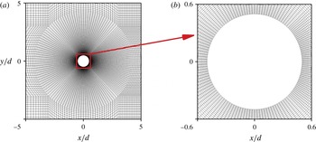
in the streamwise, cross-flow and spanwise (vertical) directions, respectively. 4 338 900 grid cells, with 32 140 grid cells in each layer perpendicular to the cylinder axis, are employed to compute the cell concentration distribution. Figure 4 shows the horizontal mesh around the circular cylinder. A check of mesh and domain dependence for two-dimensional flow in the horizontal plane, at
 $Re=100$
, is reported in appendix C. The vertical size of each grid cell is
 $0.2d$
for the region of
 $1<z/d<24$
(
 $1/25\leqslant z/H\leqslant 24/25$
, where
 $H$
is the water depth), while it is
 $0.1d$
for the region of
 $z/d\leqslant 1$
or
 $z/d\geqslant 24$
. This choice of vertical resolution is based on the fact that the characteristic length of spanwise (vertical) secondary structure is approximately
 $3d$
–
 $7d$
(Mukhopadhyay et al.
Reference Mukhopadhyay, Venugopal and Vanka1999).
Computational domain.

Horizontal mesh near the circular cylinder.

Boundary conditions;
 $n$
is the coordinate normal to the boundary.

2.3.2 Boundary and initial conditions
Boundary conditions are listed in table 1. The specified velocity
 $U_{in}(z)$
and concentration
 $C_{in}(y)$
at inlet are given by
 $$\begin{eqnarray}U_{in}(z)=U_{0}{\displaystyle \frac{z}{H}}\left(2-{\displaystyle \frac{z}{H}}\right)\end{eqnarray}$$
and
 $$\begin{eqnarray}C_{in}(y)=\left\{\begin{array}{@{}ll@{}}C_{0}, & |y/d|\leqslant 0.5,t\geqslant 0\\ 0, & |y/d|>0.5,-t_{0}\leqslant t<0,\end{array}\right.\end{eqnarray}$$
where
 $U_{0}$
is the flow velocity at the free water surface,
 $C_{0}$
is the constant concentration in the strip to which the cells are initially confined and
 $t_{0}$
is the time after which the flow no longer shows a dependence on the initial conditions. The initial flow velocity and concentration of gyrotactic organisms are set as (0, 0, 0) and 0. The non-dimensional time
 $t_{0}U_{0}/d=607.95$
is taken in the present work, according to the trial computation.
2.3.3 Parameters
The parameters used in the present work are listed in table 2. Typical values of
 $V_{s}$
,
 $B$
,
 $D_{r}$
and
 $\unicode[STIX]{x1D70F}$
of C. nivalis are taken from Pedley & Kessler (Reference Pedley and Kessler1990, Reference Pedley and Kessler1992) and Hwang & Pedley (Reference Hwang and Pedley2014b
). Since the effects of cell concentration on the ambient flow are neglected, and (2.3) is linear, the value of
 $C_{0}$
is arbitrary; we choose
 $1.0\times 10^{10}~\text{cells}~\text{m}^{-3}$
as being a reasonable value for coastal marsh land (Bratbak, Egge & Heldal Reference Bratbak, Egge and Heldal1993; Millie et al.
Reference Millie, Schofield, Kirkpatrick, Johnsen, Tester and Vinyard1997).
Parameter values. Parameter values of
 $V_{s}$
,
 $B$
,
 $D_{r}$
and
 $\unicode[STIX]{x1D70F}$
are taken from Pedley & Kessler (Reference Pedley and Kessler1990, Reference Pedley and Kessler1992), Hwang & Pedley (Reference Hwang and Pedley2014b
).

3 Results
3.1 Flow field
The major determinant of flow around a circular cylinder is the Reynolds number. In the present case, the local Reynolds number, defined as
 $Re_{local}=U_{in}d/\unicode[STIX]{x1D708}$
, varies from 0 at the bottom bed to 100 at the free water surface. There are two typical flow structures in horizontal planes: shedding vortices which are generated alternately from either side of the cylinder and travel downstream, and an approximately fixed symmetrical vortex pair in the lee of the cylinder. The vortex shedding occurs in the region above
 $z/d\approx 12.5$
, or
 $Re_{local}\approx 67$
, which is larger than the critical Reynolds number (about 49) for generating vortex shedding in uniform flow (Williamson Reference Williamson1996). Parallel shedding occurs in a region with thickness approximately
 $2d$
near the free surface, while oblique shedding occurs in the region
 $12.5\leqslant z/d<23$
.
Velocity (
 $\boldsymbol{u}/U_{0}$
) and pressure (
 $p/(0.5U_{0}^{2})$
) fields in the centreplane at
 $tU_{0}/d=157.2$
. To clearly illustrate the velocity distribution in the vicinity of the circular cylinder, the computed velocity field on the quite fine mesh is interpolated to a coarse mesh. The arrow in the white quadrilateral is the reference vector.

Oblique vortex shedding in shear flow has also been found in previous experiments (Kappler et al.
Reference Kappler, Rodi, Szepessy and Badran2005) and numerical simulations (Mukhopadhyay et al.
Reference Mukhopadhyay, Venugopal and Vanka1999). In addition, oblique shedding was found in the wake of a circular cylinder moving at a constant speed in a towing tank (Williamson Reference Williamson1989); Williamson (Reference Williamson1989) stated that this phenomenon was caused by the endplate attached to the cylinder, and that it could be manipulated by adjusting the angle of the endplate to the axis of the cylinder. A quasi-steady symmetrical vortex pair occurs below
 $z/d\approx 12.5$
, and its size in the streamwise direction decreases gradually downwards. According to the typical flow patterns described above, the wake of the cylinder can be roughly divided into three zones: the parallel-shedding zone near the water surface (
 $23\leqslant z/d\leqslant 25$
), the oblique-shedding zone (
 $12.5\leqslant z/d<23$
) and the quasi-steady zone (
 $0\leqslant z/d<12.5$
) near the bottom bed.
The flow near the cylinder shows strongly three-dimensional structure. In particular, there is a vertical (or spanwise) secondary flow in the vicinity of the cylinder, as shown in figure 5. On the leading side of the cylinder, the secondary flow is vertically downwards, and on the lee side it is vertically upwards. The non-zero vertical velocity is driven by a vertical pressure gradient (Woo et al.
Reference Woo, Cermak and Peterka1989). This arises because at the stagnation line on the front surface of the cylinder (
 $x=-0.5d$
,
 $y=0$
), Bernoulli’s theorem tells us that the pressure is
 $$\begin{eqnarray}p=p_{0}+{\textstyle \frac{1}{2}}\unicode[STIX]{x1D70C}{U_{in}}^{2}(z),\end{eqnarray}$$
where
 $p_{0}({\approx}0)$
is the uniform pressure excess (over hydrostatic) far upstream and
 $U_{in}(z)$
is given by (2.10). Hence the pressure is greater near the top surface than the bottom. At the back of the cylinder, in the region of separated flow, we have
 $$\begin{eqnarray}p\approx p_{0}-\unicode[STIX]{x1D6FE}\unicode[STIX]{x1D70C}{U_{in}}^{2}(z),\end{eqnarray}$$
a formula obtained for steady two-dimensional flow, with
 $\unicode[STIX]{x1D6FE}\approx 0.2$
for
 $Re=100$
(Fornberg Reference Fornberg1985), which is higher at the bottom than the top. These vertical pressure differences are the drivers of the computed secondary flows, as shown in figure 5. The vertical velocity becomes much weaker with distance downstream.
Variation of
 $u_{x}/U_{0}$
with
 $tU_{0}/d$
for three given points at different vertical positions with
 $x/d=4.0$
and
 $y/d=0.5$
.

Frequency spectra corresponding to figure 6;
 $A_{x}$
is the amplitude of the
 $u_{x}/U_{0}$
signal at frequency
 $f$
;
 $f_{1}=0.00635$
Hz and
 $f_{2}=0.00794$
Hz.

Variation of
 $u_{z}/U_{0}$
with
 $tU_{0}/d$
for three given points at different vertical positions with
 $x/d=4.0$
and
 $y/d=0.5$
.

Frequency spectra corresponding to figure 8;
 $A_{z}$
is the amplitude of the
 $u_{z}/U_{0}$
signal at frequency
 $f$
;
 $f_{1}=0.00635$
Hz and
 $f_{2}=0.00794$
Hz.

Frequency spectra of streamwise velocity
 $u_{z}/U_{0}$
at points with
 $x/d=1.0$
and
 $y/d=0.5$
for different vertical positions;
 $A_{z}$
is the magnitude of
 $u_{z}/U_{0}$
signal at frequency
 $f$
;
 $f_{1}=0.00635$
Hz and
 $f_{2}=0.00794$
Hz.

It was noted by Mukhopadhyay et al. (Reference Mukhopadhyay, Venugopal and Vanka1999) that the frequency of the vortex shedding in a shear flow did not vary continuously with spanwise position according to the local upstream velocity, but the flow exhibited a cellular structure along the span. In each of the cells, with lengths of approximately 6 diameters, the vortex-shedding frequency had a constant value, slightly lower than the average of the ‘expected’ values over the length of the cell, and with finite jumps over a short distance in between. To investigate the frequency structure in our flow, we have taken spectra of the three velocity components at various locations. The spectra are computed by fast Fourier transforms, based on 8400 sampling times with a sampling period of 0.3 s, corresponding to
 $tU_{0}/d\approx 0.019$
, using the values of
 $U_{0}$
and
 $d$
given in table 2. For example, figure 6 shows time traces of the dimensionless streamwise velocity
 $u_{x}/U_{0}$
at
 $x/d=4.0$
and
 $y/d=0.5$
(one cylinder radius away from the centreplane), and at three different heights. The corresponding spectra are shown in figure 7. It can be seen that there is one dominant shedding frequency,
 $f_{2}$
, in the parallel-shedding zone, and a different one,
 $f_{1}$
, in the lower part of the oblique-shedding zone. In between there is an overlap region, in which both frequencies are present (very similar results are found at other streamwise locations, but are not shown here). Besides
 $f_{1}$
and
 $f_{2}$
, a much lower frequency,
 $f_{0}$
, appears in the parallel-shedding zone and oblique-shedding zone, and it is clear that
 $f_{0}=f_{2}-f_{1}$
; this frequency represents modulation of the velocity traces in the parallel-shedding zone (see figure 6
a) – a beating frequency between the two primary oscillations. The same can be seen when we plot the vertical, or spanwise, velocities and their spectra (figures 8 and 9) (similar results are found for cross-flow velocity but are not shown here). However, when we plot the spectra of vertical velocity at a point closer to the cylinder (
 $x/d=1.0,y/d=0.5$
; figure 10), we see that the dominant frequency is
 $f_{0}$
, though its amplitude is considerably smaller than at
 $x/d=4.0$
. This indicates that the coupling between the two vortex-shedding regimes, leading to the beating (generally a weakly nonlinear process), comes about because of the presence of significant vertical velocities, i.e. the secondary flows already discussed. We may note that a similar phenomenon of beating in the velocity fluctuation spectra was observed experimentally by Williamson (Reference Williamson1989), who also explained it as resulting from the interaction of two higher frequencies.
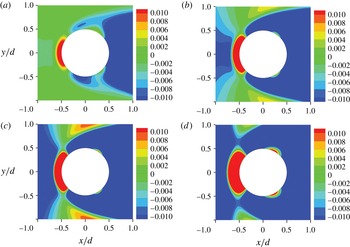
Contours of
 $\unicode[STIX]{x1D714}_{\unicode[STIX]{x1D719}}B$
around the circular cylinder at
 $tU_{0}/d=157.2$
: (a)
 $z/d=24$
, (b)
 $z/d=20$
, (c)
 $z/d=15$
and (d)
 $z/d=2.5$
.
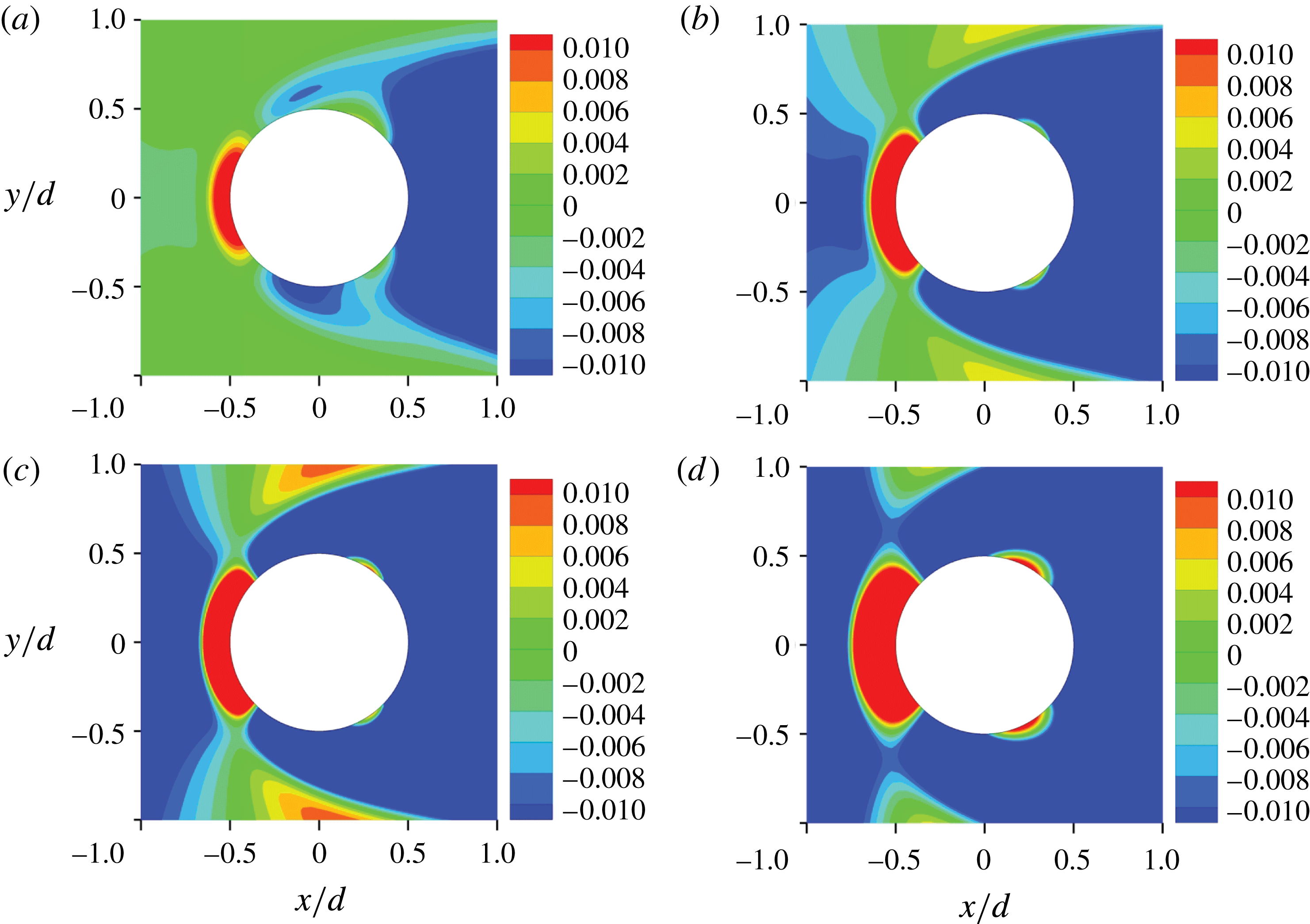
Corresponding to the typical characteristics of the velocity distribution, the vorticity exhibits a range of behaviour according to the spanwise position. In the parallel-shedding zone, the vortex shedding is close to two-dimensional. The vertical vorticity is much larger than the horizontal vorticity. The weak vorticity in the cross-flow (
 $y$
-) direction at first gradually increases with downstream distance, but later dies away due to viscous dissipation.
In the oblique-shedding zone, strong three-dimensional vorticity is evident. The streamwise and vertical vorticities are comparable with each other. The oblique vortices link well with the approximately parallel vortices in the parallel-shedding zone in the region near the cylinder.
In the quasi-steady zone, none of the three vorticity components changes significantly with time and they are symmetrical with respect to the centreplane. The streamwise and spanwise vorticity components become weaker at smaller values of
 $z$
, due to the lower incoming velocity near the bottom of the channel, while the cross-flow vorticity becomes strong there, due to the higher shear of the incident flow.
Positive circumferential vorticity
 $\unicode[STIX]{x1D714}_{\unicode[STIX]{x1D719}}$
, defined as
 $$\begin{eqnarray}\unicode[STIX]{x1D714}_{\unicode[STIX]{x1D719}}={\displaystyle \frac{\unicode[STIX]{x2202}u_{r}}{\unicode[STIX]{x2202}z}}-{\displaystyle \frac{\unicode[STIX]{x2202}u_{z}}{\unicode[STIX]{x2202}r}},\end{eqnarray}$$
where
 $u_{z}$
and
 $u_{r}$
are the vertical and radial velocity components, and
 $r$
is the radial distance from the cylinder axis, mainly occurs in the area around the upstream stagnation point at all spanwise positions (except close to the water surface and the bottom bed), while negative circumferential vorticity dominates the remainder of the cylinder surface, as shown in figure 11. On the surface of the cylinder
 $\unicode[STIX]{x2202}u_{r}/\unicode[STIX]{x2202}z=0$
, so the sign of
 $\unicode[STIX]{x1D714}_{\unicode[STIX]{x1D719}}$
is opposite to that of the vertical (secondary) velocity, from (3.3).
3.2 Mean swimming velocity and translational diffusivity
In the present case, the p.d.f. of swimming direction,
 $f(\boldsymbol{p})$
, is taken to be quasi-steady, as discussed at the end of § 2.1, and therefore satisfies equation (2.9) without the
 $\unicode[STIX]{x2202}f/\unicode[STIX]{x2202}t$
term. (We actually solve the equation retaining the
 $\unicode[STIX]{x2202}f/\unicode[STIX]{x2202}t$
term with a particular initial condition, and use the solution after it becomes steady.) We consider values of the vorticity vector that satisfy
 $B\sqrt{\unicode[STIX]{x1D714}_{x}^{2}+\unicode[STIX]{x1D714}_{y}^{2}}<1$
, so cells do not tumble and there is no possibility of cell trapping by shear (Durham et al.
Reference Durham, Kessler and Stocker2009). The Fokker–Planck equation (2.9) is solved for a particular value of
 $\unicode[STIX]{x1D74E}$
and the corresponding mean swimming velocity
 $\boldsymbol{V}_{c}$
and translational diffusivity
 $\unicode[STIX]{x1D63F}$
are obtained from equations (2.4) and (2.6) respectively.
When the vorticity is very small, so
 $\left|B\unicode[STIX]{x1D74E}\right|<0.02$
, the swimming velocity and translational diffusivity are directly calculated from the analytical solution of Pedley & Kessler (Reference Pedley and Kessler1990), which can be rewritten in the current notation as
 $$\begin{eqnarray}{\displaystyle \frac{\boldsymbol{V}_{c}}{V_{s}}}=(0.45B\unicode[STIX]{x1D714}_{y},-0.45B\unicode[STIX]{x1D714}_{x},0.57),\end{eqnarray}$$
and
 $$\begin{eqnarray}{\displaystyle \frac{\unicode[STIX]{x1D63F}}{V_{s}^{2}\unicode[STIX]{x1D70F}}}=\left[\begin{array}{@{}ccc@{}}0.26 & 0 & -0.10B\unicode[STIX]{x1D714}_{y}\\ \displaystyle 0 & 0.26 & -0.10B\unicode[STIX]{x1D714}_{x}\\ \displaystyle -0.10B\unicode[STIX]{x1D714}_{y} & -0.10B\unicode[STIX]{x1D714}_{x} & 0.16\\ \end{array}\right].\end{eqnarray}$$
However, when
 $|B\unicode[STIX]{x1D74E}|>0.02$
,
 $\boldsymbol{V}_{c}$
and
 $\unicode[STIX]{x1D63F}$
are calculated from a database that we set up for these quantities in the three-dimensional vorticity space. This is established by solving the Fokker–Planck equation 4901 times, with the same initial condition, i.e.
 $f=1/4\unicode[STIX]{x03C0}$
, for a set of vorticities
 $(\unicode[STIX]{x1D714}_{1}^{j},\unicode[STIX]{x1D714}_{2}^{k},\unicode[STIX]{x1D714}_{3}^{l})$
(
 $j=1,2\ldots 13$
,
 $k=1,2\ldots 13$
and
 $l=1,2\ldots 29$
) subject to
 $$\begin{eqnarray}B\unicode[STIX]{x1D714}_{i}^{j}=\left\{\begin{array}{@{}ll@{}}-2^{j}/100, & i=1,2,\quad j=1\ldots 6\\[2.0pt] 0, & i=1,2,\quad j=7\\[2.0pt] 2^{j-7}/100, & i=1,2,\quad j=8\ldots 13\end{array}\right.\end{eqnarray}$$
and
 $$\begin{eqnarray}B\unicode[STIX]{x1D714}_{i}^{j}=\left\{\begin{array}{@{}ll@{}}-2^{j}/100, & i=3,\quad j=1\ldots 14\\[2.0pt] 0, & i=3,\quad j=15\\[2.0pt] 2^{j-15}/100, & i=3,\quad j=16\ldots 29,\end{array}\right.\end{eqnarray}$$
where
 $i$
represents the
 $i$
th component of vorticity. The vorticity in the database (
 $|B\unicode[STIX]{x1D714}_{x}|\leqslant 0.64$
,
 $|B\unicode[STIX]{x1D714}_{y}|\leqslant 0.64$
, and
 $|B\unicode[STIX]{x1D714}_{z}|\leqslant 163.84$
), covers the whole range of vorticity found for the present flow round a circular cylinder. It is noted that the database is specific only to C. nivalis with
 $B=3.4$
s and
 $D_{r}=0.067~\text{s}^{-1}$
.
Contours of swimming velocity and vorticity at
 $z/d$
= 20: (a)
 $V_{x}/V_{s}$
, (b)
 $B\unicode[STIX]{x1D714}_{y}$
, (c)
 $V_{y}/V_{s}$
, (d)
 $B\unicode[STIX]{x1D714}_{x}$
and (e)
 $V_{z}/V_{s}$
.

In our principal computation, the mean swimming velocity and translational diffusivity tensor are updated at each time step by linear interpolation in the database of
 $\boldsymbol{V}_{c}-\unicode[STIX]{x1D74E}$
and
 $\unicode[STIX]{x1D63F}-\unicode[STIX]{x1D74E}$
, as well as by the analytical solution for the steady Fokker–Planck equation for small
 $|B\unicode[STIX]{x1D74E}|$
.
In the parallel-shedding zone, the mean swimming velocity components in the horizontal directions are much smaller than that in the vertical (spanwise) direction, which means that cells swim almost vertically upwards. There is no obvious variation of horizontal swimming velocity in the wake of the cylinder, which is attributable to the weak streamwise and cross-flow vorticity in this zone.
In the oblique-shedding zone, the distribution of streamwise mean swimming velocity is matched with the corresponding distribution of the cross-flow vorticity, while the distribution of cross-flow mean swimming velocity is matched with the corresponding distribution of the streamwise vorticity, as shown in figure 12. In the upper portion of this region, the magnitude of the horizontal mean swimming velocity is much smaller than that of the vertical mean swimming velocity, but varies noticeably in the wake of the cylinder. As we would expect, the vertical mean swimming velocity in the wake of the cylinder is smaller than that outside the wake, due to the influence of horizontal vorticity.
In the quasi-steady zone, the horizontal mean swimming velocity is generally smaller than that in the oblique-shedding zone. The small horizontal mean swimming velocity in this zone was caused by the weak incoming velocity, in contrast to that in the parallel region caused by the weak shear of the incoming flow.
To characterise the relative importance of mirco-organism swimming and ambient flow, we define the relative swimming velocity
 $\unicode[STIX]{x1D6FD}_{i}$
as
 $$\begin{eqnarray}\unicode[STIX]{x1D6FD}_{i}={\displaystyle \frac{|V_{i}|}{|u_{i}|+\unicode[STIX]{x1D716}}},\end{eqnarray}$$
where
 $V_{i}$
and
 $u_{i}$
are the
 $i$
th components of the mean swimming velocity and flow velocity, respectively, and
 $\unicode[STIX]{x1D716}$
, taken as
 $10^{-3}~\unicode[STIX]{x03BC}\text{m}~\text{s}^{-1}$
, is included to avoid the singularity caused when
 $u_{i}=0$
.
In the parallel-shedding zone,
 $\unicode[STIX]{x1D6FD}_{x}\approx 0.08$
,
 $\unicode[STIX]{x1D6FD}_{y}\approx 0.10$
and
 $\unicode[STIX]{x1D6FD}_{z}\approx 0.9$
, which implies that the horizontal advective transport of cells is dominated by advection with the ambient flow, and that the contribution of the vertical mean swimming velocity is comparable with that of the vertical fluid velocity.
Contours of
 $\unicode[STIX]{x1D6FD}_{z}$
at
 $z/d=0$
, 5, 10, 15, 20 and 25.

Contours of
 $V_{r}/V_{s}$
around the circular cylinder at
 $U_{0}t/d=157.2$
: (a)
 $z/d=24$
, (b)
 $z/d=20$
, (c)
 $z/d=15$
and (d)
 $z/d=2.5$
.

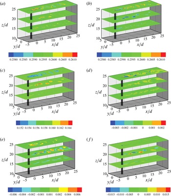
Contours of diffusivity tensor at
 $z/d$
= 15, 20 and 25: (a)
 $D_{xx}/(V_{s}^{2}\unicode[STIX]{x1D70F})$
, (b)
 $D_{yy}/(V_{s}^{2}\unicode[STIX]{x1D70F})$
, (c)
 $D_{zz}/(V_{s}^{2}\unicode[STIX]{x1D70F})$
, (d)
 $D_{xy}/(V_{s}^{2}\unicode[STIX]{x1D70F})$
, (e)
 $D_{xz}/(V_{s}^{2}\unicode[STIX]{x1D70F})$
and (f)
 $D_{yz}/(V_{s}^{2}\unicode[STIX]{x1D70F})$
. Note that the colour scales are different for different panels.

In the oblique-shedding zone, the ambient flow still overwhelms the horizontal mean swimming. In the vortex cores, the vertical flow is stronger than the vertical swimming, while, just outside the cores, the vertical swimming is comparable with the vertical flow, i.e.
 $|\unicode[STIX]{x1D6FD}_{z}|=O(1)$
as shown in figure 13. As
 $z$
decreases, the importance of the vertical relative swimming gradually increases due to the decreasing incident velocity.
In the quasi-steady zone, the horizontal mean swimming velocity in the streamwise direction is much smaller than the horizontal flow velocity except in the region next to the bed bottom; the vertical mean swimming velocity and vertical flow are comparable with each other.
On the surface of the cylinder, except very near the water surface and the bottom bed, the dimensionless radial mean swimming velocity,
 $V_{r}/V_{s}$
, is directed outwards on the leading side of the cylinder and inwards in the lee of the cylinder, as shown in figure 14. This distribution of radial mean swimming velocity is consistent with the distribution of
 $\unicode[STIX]{x1D714}_{\unicode[STIX]{x1D719}}$
(figure 11), and can be understood from the steady-state solution of (2.8):
 $$\begin{eqnarray}\sin \unicode[STIX]{x1D703}=B\unicode[STIX]{x1D714}_{\unicode[STIX]{x1D719}},\end{eqnarray}$$
where
 $\unicode[STIX]{x1D714}_{\unicode[STIX]{x1D719}}$
is the non-zero horizontal component of vorticity and
 $\boldsymbol{p}=(\sin \unicode[STIX]{x1D703},0,\cos \unicode[STIX]{x1D703})$
.
In the present case, the orders of magnitude of the diagonal components of the translational diffusivity tensor are much greater than those of the off-diagonal components in the wake of the cylinder, as shown in figure 15, which means that the cell flux by translational diffusion through a plane mainly depends on the concentration gradient normal to that plane. (Note that the colour scales vary between the panels of figure 15 in order to emphasise the zones in which the different components of
 $\unicode[STIX]{x1D63F}$
are greatest.) The diagonal components
 $D_{xx}$
,
 $D_{yy}$
and
 $D_{zz}$
vary to some extent in the present work, in contrast to the constant value for an ambient flow with
 $B|\unicode[STIX]{x1D74E}|\ll 1$
(Pedley & Kessler Reference Pedley and Kessler1990). The order of magnitude of
 $D_{yz}$
is greater than that of
 $D_{xy}$
.
Variation of
 $C/C_{0}$
with
 $tU_{0}/d$
for positions
 $y/d=0.0$
: (a)
 $x/d=-8.0$
, (b)
 $x/d=1.0$
and (c)
 $x/d=8.0$
. Green colour represents
 $z/d=24$
or
 $z/H=0.95$
; red colour represents
 $z/d=12.5$
or
 $z/H=0.5$
.

3.3 Three-dimensional distribution of gyrotactic micro-organisms and passive particles
Here we compute the concentration distribution of motile cells, and compare the results with those for passive particles that are advected without diffusion, and for passive particles that are advected in the presence of isotropic diffusion with diffusivity
 $D=V_{s}^{2}\unicode[STIX]{x1D70F}/3$
. The strip of incoming motile micro-organisms (C. nivalis) spreads little in the cross-flow direction until the particles come close to the cylinder. This is the same as for passive particles, as shown in figure 16(a), where the particle concentration is plotted against time for a position on the centre plane 8 diameters upstream of the cylinder axis. The weak variation of cell concentration upstream is explained by the large time scale,
 $O(d^{2}/D_{yy})=3.1\times 10^{5}~\text{s}$
, for diffusion across the width of the strip
 $d=4$
cm by translational diffusion, compared to the time scale,
 $O(L_{0}/U_{0})=320~\text{s}$
, for travelling to the cylinder by advection from upstream, where
 $L_{0}$
is the distance from the upstream inlet to the axis of the cylinder.
Distribution of
 $C/C_{0}$
for
 $z/d=5$
, 10, 15, 20 and 25 at
 $tU_{0}/d=157.2$
: (a) active particles, and (b) passive particles without diffusion.

Variation of
 $Q_{c}$
with
 $tU_{0}/D$
.

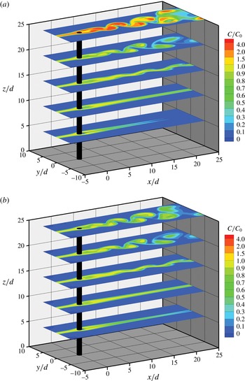
The presence of the cylinder greatly changes the dispersion of both active and passive particles. In the parallel-shedding zone, both active and passive particles travel downstream in the pattern of the shed vortex street rather than the initial strip distribution, forming alternating concentrated regions on either side of the wake, as shown in figure 17. The general pattern of the concentration distribution is quite similar for active and passive particles, which means that the horizontal transport of particles in this zone is dominated by advection, which is consistent with the result that the mean swimming velocity is quite weak compared with the ambient flow. However, the maximum concentration of active particles occurs at the upper surface of the fluid, in the wake region, and greatly exceeds that in the upstream strip, as shown by the red patches on the top surface in figure 17(a), while that of passive particles does not. The reason for this difference lies in the fact that the active particles can swim across streamlines and accumulate at the free surface while the passive particles cannot. The obvious accumulation of active particles in the top layer near the water surface shows that vertical swimming plays an important role. This is in good agreement with the result that the values of
 $\unicode[STIX]{x1D6FD}_{z}$
are close to 1 (figure 13).
The effects of cell swimming on the total number of particles that accumulate in the top layer are also shown in figure 18, where
 $Q_{c}$
is defined as
 $$\begin{eqnarray}Q_{c}={\displaystyle \frac{1}{C_{0}V_{0}}}\iiint _{V}C(x,y,z,t)\,\text{d}x\,\,\text{d}y\,\text{d}z,\end{eqnarray}$$
and
 $$\begin{eqnarray}V_{0}=\iiint _{V}\,\text{d}x\,\text{d}y\,\text{d}z.\end{eqnarray}$$
The domain of integration,
 $V$
, is defined as
 $-20\leqslant x/d\leqslant 40$
,
 $-0.5\leqslant y/d\leqslant 0.5$
and
 $24.5\leqslant z/d\leqslant 25$
, so
 $Q_{c}$
represents the ratio of the number of cells in the top
 $0.5d$
to the corresponding number if
 $C=C_{0}$
everywhere. It is interesting that, although the concentration of active particles is very large at the free surface behind the cylinder, it is actually significantly lower than that of passive particles at mid-depth, as shown in figure 16(b) (red curves). However, this difference does not persist downstream (at
 $x/d=8.0$
) as shown in figure 16(c). At particular points the concentrations of active and passive particles oscillate dramatically, as shed vortices sweep past, bringing particle-free fluid from outside the strip across the centre plane. This can be seen clearly in figures 16(c) and 17, for example.
In the upper part of the oblique-shedding zone, both active and passive particle clouds travel downstream in the pattern of an oblique vortex street, while in the lower part of this zone the particle clouds travel in a pattern that resembles a fluttering ribbon, as shown in figure 17. The general pattern of concentration distribution implies that the shape of particle clouds in the horizontal plane is mainly determined by advection, which is consistent with the fact that the cell swimming velocity is much smaller than the horizontal components of the flow velocity. However, there is still an effect of vertical swimming on the concentration distribution, as shown in figure 16(b,c), because the vertical components of swimming and flow velocity are comparable.
Distribution of
 $C/C_{0}$
for
 $y/d=0.0$
at
 $tU_{0}/d=157.2$
: (a) active particles, and (b) passive particles without diffusion. For description of black and white bold lines, see text.

Distribution of
 $C/C_{0}$
for
 $z/d=20$
(b,d) and 23 (a,c) at
 $tU_{0}/d=157.2$
: (a,b) active particles, and (c,d) passive particles without translational diffusion.

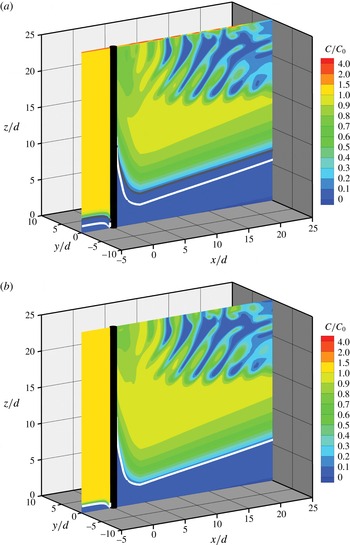
In the quasi-steady zone, the particle concentration distribution is approximately symmetric with respect to the wake centreplane (figure 17). There is a low concentration of cells immediately behind the cylinder because the concentration was initially zero, and neither swimming nor diffusion has brought particles into that zone by the time depicted in figure 17. Moreover, upswimming (of active particles) tends to remove particles from that zone. Further out, in the
 $y$
-direction, swimming and translational diffusion smooth out the interface between the low concentration behind the cylinder and the outer region. Both active and passive particles move downward slightly on the leading side of the cylinder near the bed bottom, due to the downward flow velocity, as shown in figure 19. The boundary of the active particle cloud, represented by a black bold line in figure 19(a) is above that of the passive particle cloud, represented by a white bold line in figure 19(b), due to the upward swimming of active particles.
Another striking difference between the concentration distributions of passive and active particles is found in a thin layer adjacent to the circular cylinder, as shown in figure 20. For the active particles, a high concentration region occurs in the lee of the cylinder, while a low concentration region appears on the leading side (see figure 20 b in particular). The concentration variation in this thin layer is caused by radial swimming (see figure 14), in contrast to the high concentration layer of active particles at the top surface which is a consequence of upward swimming (figure 17 a). No high concentration layer was found on the cylinder for passive particles.
We should note that figures 17(b), 19(b) and 20(c,d) are for passive particles without diffusion. Corresponding plots for passive particles with isotropic diffusion are indistinguishable from these and are therefore not presented. It is clear that isotropic diffusion with
 $D={V_{s}}^{2}\unicode[STIX]{x1D70F}/3$
would have negligible effect in this flow.
4 Discussion
It is intended that this paper will be the first in a series to investigate tidal fluid flow and the distribution of motile micro-organisms in coastal wetlands populated by emergent vegetation, characterised by tall stems which may be branched but not leafy under water. An important aim of the paper has therefore been to develop a computational platform for solving the problems that arise: compute the fluid flow from the Navier–Stokes equations; assume a dilute suspension of swimming cells, but in a continuum description, and compute their orientation distribution by solving a Fokker–Planck equation that involves the torque applied to the cells by vorticity in the flow, and hence set up a database of mean cell swimming velocity and translational diffusivity as functions of that vorticity; and finally solve the cell conservation equation for the cell population density. As a first example, we have considered the highly idealised model of a horizontal shear flow past a single vertical, rigid, circular cylinder of diameter
 $d$
, that is fixed in the bottom bed of a parallel-sided channel and extends through the whole depth of the fluid; the Reynolds number at the free surface was taken to be 100. The cells that have been considered are gyrotactic motile algae such as C. nivalis that are bottom heavy and swim upwards on average when there is no flow. The inflowing cells were taken to occupy a vertical strip of width
 $d$
; this is clearly unrealistic but permits an examination of the effect of the cylinder and of gyrotaxis on such lateral inhomogeneity. The distribution of active particles (cells) was compared with that for passive particles.
The main results were as follows. First of all, the flow field downstream of the cylinder is dominated by vortex shedding, in three zones: parallel shedding near the top surface, where the incoming shear rate is small; oblique shedding below that; and quasi-steady separated flow near the bottom. The zones are coupled in part by a mean secondary flow, downwards just upstream of the cylinder and upwards just downstream (figure 5). These findings are qualitatively consistent with those of previous authors (Williamson Reference Williamson1989; Woo et al.
Reference Woo, Cermak and Peterka1989; Mukhopadhyay et al.
Reference Mukhopadhyay, Venugopal and Vanka1999). The magnitude of the streamwise component of vorticity is comparable to that of the spanwise (vertical) component in the oblique-shedding zone. Near the cylinder surface the horizontal component of the vorticity is circumferential (
 $\unicode[STIX]{x1D714}_{\unicode[STIX]{x1D719}}$
); this component is positive in the neighbourhood of the upstream stagnation line and negative almost everywhere else on the surface (figure 11). These signs are consistent with the signs of the secondary flow velocity in the corresponding locations.
Perhaps the most interesting aspects of the flow field are the time spectra of the velocity components in the vortex-shedding zones. The parallel-shedding zone is dominated by one frequency,
 $f_{2}$
(see figure 7, for example), and the oblique-shedding zone is dominated by another,
 $f_{1}$
; where the zones overlap, there is a marked contribution from the beating frequency,
 $f_{0}=f_{2}-f_{1}$
(see figures 7 and 9;
 $f_{0}$
in fact dominates the spectrum of the vertical velocity component (figure 10). It is interesting that these dominant frequencies do not vary with
 $z$
. This, together with the existence of the beating frequency, is clear evidence of nonlinear vortex dynamics.
The mean swimming velocity and translational diffusivity tensor of the cells were computed for organisms with
 $(2BD_{r})^{-1}=2.2$
(e.g. C. nivalis), and for vorticity vectors such that
 $|B\unicode[STIX]{x1D714}_{x}|<0.64$
,
 $|B\unicode[STIX]{x1D714}_{y}|<0.64$
and
 $|B\unicode[STIX]{x1D714}_{z}|<163.84$
. The computations were based on a combination of the analytical solution by Pedley & Kessler (Reference Pedley and Kessler1990) and numerical solutions of the steady Fokker–Planck equation. The results were stored in a database of
 $\boldsymbol{V}_{c}-\unicode[STIX]{x1D74E}$
and
 $\unicode[STIX]{x1D63F}-\unicode[STIX]{x1D74E}$
, and the mean cell swimming velocity and translational diffusivity tensor in the flow around the cylinder were obtained from that database. In the whole region, with the exception of the bottom bed and the surface of the cylinder, the ambient flow overwhelms cell swimming in the horizontal direction. In the parallel-shedding zone, cells swim almost vertically upwards in the wake of the cylinder due to the weak streamwise and cross-flow vorticity. In the oblique-shedding zone, the vertical flow dominates the vertical migration of cells in the vortex cores, while outside the cores and in the quasi-steady zone vertical swimming is comparable to the vertical flow. The distribution of radial mean swimming velocity is consistent with the distribution of
 $\unicode[STIX]{x1D714}_{\unicode[STIX]{x1D719}}$
. In the wake of the cylinder, the orders of magnitude of the diagonal components of the translational diffusivity tensor are much greater than those of the off-diagonal components, meaning that the cell flux by translational diffusion through a plane is almost proportional to the normal component of the concentration gradient.
The incoming strip of particles, either active or passive, spreads little in the cross-flow direction until the particles are close to the cylinder. In the parallel-shedding zone (except at the very top surface), the general pattern of the concentration distribution is quite similar for both active and passive particles, which means that the horizontal transport of particles in this zone is dominated by advection. However, the maximum concentration of active particles in the wake region occurs at the top surface, and exceeds the initial concentration, while that of passive particles does not. This difference is attributable to the cells’ ability to swim across streamlines. In the upper part of the oblique-shedding zone, both active and passive particle clouds travel downstream in the pattern of the oblique vortex street, while in the lower part of this zone, the particle clouds more resemble a fluttering ribbon. The effect of vertical swimming on the concentration distribution is still observed in the oblique-shedding region. In the quasi-steady zone, the particle concentration distribution is approximately symmetric with respect to the wake centreplane. Swimming and translational diffusion of cells smooth out the sharp concentration interface in the rear of the cylinder. The region of zero cell concentration above the bottom bed is deeper for active particles than for passive particles, due to vertical swimming. Another striking difference between passive and active particles is that a high concentration region of swimming cells occurs in the lee of the cylinder, which is caused by the radial swimming velocity rather than the spanwise swimming that takes place in the thin layer near the water surface.
This discussion will now address two major concerns: the validity of the assumptions and approximations that have been made in solving the model problem, and the relevance of the model problem to wetland flows.
First, the presence of the cells has been ignored in the Navier–Stokes equation (2.2): the (negative) buoyancy term would be
 $Cgv\unicode[STIX]{x0394}\unicode[STIX]{x1D70C}/\unicode[STIX]{x1D70C}$
, where
 $v$
is cell volume,
 $\unicode[STIX]{x0394}\unicode[STIX]{x1D70C}/\unicode[STIX]{x1D70C}$
is the relative density difference between cells and water and
 $g$
is gravity, and the contribution from the divergence of the ‘particle stress tensor’ scales as
 $4CTa/\unicode[STIX]{x1D70C}d$
, where
 $T$
is the thrust exerted by a cell (equal to its drag),
 $a$
is the cell radius and
 $C$
is the number density of cells. Using values from table 2 and Pedley & Kessler (Reference Pedley and Kessler1990), the ratios of these to the Newtonian viscous term
 $\unicode[STIX]{x1D708}\unicode[STIX]{x1D6FB}^{2}\boldsymbol{u}$
are approximately 0.17 and 0.03 respectively when
 $C\approx 10^{4}~\text{cm}^{-3}$
. This value of
 $C$
is lower than that which leads to bioconvection in the laboratory (Pedley & Kessler Reference Pedley and Kessler1992) but larger than values normally found in the field (Bratbak et al. (Reference Bratbak, Egge and Heldal1993) and Millie et al. (Reference Millie, Schofield, Kirkpatrick, Johnsen, Tester and Vinyard1997) found maximum concentrations of
 $5\times 10^{3}$
cells
 $\text{cm}^{-3}$
and
 $1.2\times 10^{4}$
cells
 $\text{cm}^{-3}$
, respectively, during algal blooms of two different species). Thus the neglect of these terms is justified as a first approximation, but the gravitational term, in particular, may lead to new effects on non-horizontal boundaries.
We have already discussed, in § 2.1, the conditions for the p.d.f. of swimming direction to be quasi-steady and quasi-uniform, i.e. the time derivative and advective terms to be negligible in the Fokker–Planck equation (2.7), leading to (2.9). Using the parameter values given in table 1, these conditions are met only very approximately. However, in order to solve (2.7) exactly, the cell velocity
 $\dot{\boldsymbol{x}}$
and the local vorticity
 $\unicode[STIX]{x1D74E}$
would have to be updated at every time step, which would require the velocity and vorticity fields to be recorded throughout the computation, and this is still beyond the realistic capability even of supercomputers. The problem would be less troublesome if the flow were effectively independent of time, which may be relevant in an array of cylinders (see below) or at much lower Reynolds numbers. A side issue is that we have assumed that the vorticity is nowhere large enough to cause cell tumbling, i.e.
 $|(\unicode[STIX]{x1D74E}-\unicode[STIX]{x1D714}_{z}\boldsymbol{k})|B<1$
; that this is satisfied is demonstrated in figure 12.
Another important assumption is of the validity of the continuum model itself. This requires that length scales over which the flow varies should be greater than a typical spacing between the cells. For the quoted cell density of
 $10^{4}$
per cm
 $^{3}$
the average spacing is about 400–
 $500~\unicode[STIX]{x03BC}\text{m}$
; this is less than the length scales that appear in the flow, although not much less in the interesting zone just behind the cylinder (figure 20
b). For significantly smaller cell number densities, it would be necessary to use an individual-based model, not a continuum model (see Hopkins & Fauci Reference Hopkins and Fauci2002, Thorn & Bearon Reference Thorn and Bearon2010, De Lillo et al.
Reference De Lillo, Cencini, Durham, Barry, Stocker, Climent and Boffetta2014).
We also return briefly to the approximation (2.6) for the translational diffusivity tensor. Hill & Bees (Reference Hill and Bees2002) developed generalised Taylor dispersion (GTD) theory for gyrotactic cells (see Croze et al. (Reference Croze, Bearon and Bees2017), appendix A, or Bearon et al. (Reference Bearon, Bees and Croze2012) for a succinct statement of how to calculate
 $\unicode[STIX]{x1D63F}$
in GTD theory). They showed in particular that, for a linear shear flow in the
 $x$
-direction with vorticity in the
 $y$
-direction, this theory predicts that all components of
 $\unicode[STIX]{x1D63F}$
, except
 $D_{yy}$
, tend to zero as the vorticity tends to infinity, whereas (2.6) predicts that all components tend to non-zero constants in that limit; for relatively small vorticity, on the other hand, equation (2.6) agrees quite well with GTD theory. These results were later confirmed by comparing the predictions with an individual-based model (Croze et al.
Reference Croze, Sardina, Ahmed, Bees and Brandt2013) and with experiment (Croze et al.
Reference Croze, Bearon and Bees2017). However, it remains the case that even GTD theory agrees poorly with an individual-based simulation in strain-dominated flows, because the velocity gradient (assumed uniform in the theory) can vary rapidly with position (Bearon et al.
Reference Bearon, Hazel and Thorn2011), and straining cannot be neglected in the flow patterns that we have computed in this paper. In the future, we should either use GTD theory or embark on individual-based simulations.
The discussion and references in the introduction indicate that a rigid cylinder is not a bad model for grasses such as S. alterniflora, although the stems do branch towards the upper surface; in particular the chosen Reynolds number is in a realistic range. However, such stems are flexible to some extent, and bend in the flow; other grasses with thinner stems will be significantly deformed by flow. The greatest bending moment experienced by the vertical cylinder in our model will occur at the base, where it will be equal to
 $$\begin{eqnarray}M={\displaystyle \frac{1}{2}}\unicode[STIX]{x1D70C}d\int _{0}^{H}~C_{d}(z)(U_{in}(z))^{2}z\,\text{d}z,\end{eqnarray}$$
where
 $C_{d}$
is the
 $z$
-dependent drag coefficient and
 $U_{in}(z)$
is given by (2.10), and we have assumed that the drag per unit length at height
 $z$
is the same as for an infinite cylinder in a velocity
 $U_{in}(z)$
.
 $C_{d}$
would vary from about 1.3 at the top, where
 $Re=100$
, to about 2.2 at
 $z/H=0.1$
where
 $Re\approx 19$
(Batchelor Reference Batchelor1967, figure 4.12.7). Rather than aspire to complete accuracy, we recognise that the contributions from larger
 $z$
will dominate
 $M$
, and arbitrarily choose
 $C_{d}=1.5$
in the above equation. Using the parameter values given in table 2, therefore, we obtain
 $M\approx 7.8\times 10^{-5}~\text{kg}~\text{m}^{2}~\text{s}^{-2}$
.
The radius of curvature of a rod at any point is equal to its bending stiffness
 $\unicode[STIX]{x1D6F4}$
divided by the bending moment at that point. Feagin et al. (Reference Feagin, Irish, Möller, Williams, Colón-Rivera and Mousavi2011) gave data for S. alterniflora from which we can deduce a bending stiffness of
 $\unicode[STIX]{x1D6F4}\approx 2.35\times 10^{-2}~\text{N}~\text{m}^{2}$
, while Hamann & Puijalon (Reference Hamann and Puijalon2013) measured
 $\unicode[STIX]{x1D6F4}$
for several other emergent aquatic plants, and found values in the range
 $10^{-3}<\unicode[STIX]{x1D6F4}<10^{-1}~\text{N}~\text{m}^{2}$
. Hence the radius of curvature
 $\unicode[STIX]{x1D6F4}/M$
at the base of the stem in our case would be greater than 10 m. Thus the drag force exerted by a stream of maximum speed
 $U_{0}=2.5\times 10^{-3}~\text{m}~\text{s}^{-1}$
(table 2) will not be enough to bend the stems significantly. (We should nevertheless bear in mind that
 $M$
is proportional to
 ${U_{0}}^{2}$
, so it would only take a stream of
 $2.5\times 10^{-2}~\text{m}~\text{s}^{-1}$
to give
 $\unicode[STIX]{x1D6F4}/M$
between 0.1 and 10 m, the smaller of which represents considerable bending.)
A further implicit assumption of our model is that, in a saltmarsh with emergent vegetation, there is no significant effect on the flow from external sources, such as oceanic turbulence or waves, including locally wind-driven waves as well as those propagating in from the ocean. Especially in marshes in which the grasses are close together and do not deform significantly, it seems obvious that turbulence in the incoming flow will die away quickly with distance from the leading edge of the vegetation. Some authors of papers in this field use the word turbulence to describe the flow resulting from time-dependent vortex shedding from the stems of the plants. Following Lightbody & Nepf (Reference Lightbody and Nepf2006) we do not call this turbulence; although the interaction between such vortices will produce a very complex flow, it is precisely this flow that we will wish to investigate in future work.
The importance of surface waves is more difficult to assess. Waves are clearly significant for seagrass meadows that are fully submerged, especially when the grasses are long and very flexible (and exhibit beautiful wave patterns themselves); see Luhar et al. (Reference Luhar, Coutu, Infantes, Fox and Nepf2010), for example. In the emergent case, as for turbulence, very short waves coming from upstream will be damped out quickly, and the part of the vegetation above water will suppress the local generation of waves by the wind (if the subsurface vegetation is effectively rigid). However, there remain fairly long waves coming in from the ocean. Consider an incoming, sinusoidal, shallow-water wave of wave speed
 $c=\sqrt{gH}$
, height amplitude
 $h_{0}$
and corresponding velocity amplitude
 $u_{0}=\sqrt{g/H}h_{0}$
which we take to be large compared with the underlying shear flow velocity
 $U_{0}$
. Then the drag on a single cylinder is
 $F_{D}=(1/2)\unicode[STIX]{x1D70C}dHC_{d}U^{2}$
, where
 $U$
is the instantaneous, depth-averaged flow speed, and the rate at which energy is lost as a result of the drag is
 $|U|F_{D}$
. We assume that the reedbed consists of
 $N$
identical cylinders, evenly spaced per unit horizontal area (p.u.h.a.). Hence the mean rate of energy loss p.u.h.a. is
 $$\begin{eqnarray}\overline{W}={\textstyle \frac{1}{2}}\unicode[STIX]{x1D70C}\,dHC_{d}\overline{|U|^{3}}N,\end{eqnarray}$$
which scales as
 $\unicode[STIX]{x1D70C}dH{u_{0}}^{3}N$
, ignoring multiplicative constants of
 $O(1)$
(see Dean & Bender (Reference Dean and Bender2006) for example). Now the mean energy in the waves,
 $\overline{E}$
p.u.h.a., scales as
 $\unicode[STIX]{x1D70C}g{h_{0}}^{2}$
so
 $\text{d}\overline{E}/\text{d}t=-\overline{W}$
, with the result that
 $$\begin{eqnarray}\unicode[STIX]{x1D70C}g{\displaystyle \frac{\text{d}{h_{0}}^{2}}{\text{d}t}}=-\unicode[STIX]{x1D70C}\,dg\sqrt{{\displaystyle \frac{g}{H}}}N{h_{0}}^{3},\end{eqnarray}$$
and hence
 $$\begin{eqnarray}h_{0}={\displaystyle \frac{h_{00}}{1+{\textstyle \frac{1}{2}}h_{00}\unicode[STIX]{x1D70E}t}},\end{eqnarray}$$
where
 $\unicode[STIX]{x1D70E}=d\sqrt{g/H}N$
and
 $h_{00}$
is the initial amplitude. For
 $H=1.0$
m,
 $d=2.5\times 10^{-3}$
m and
 $N=200~\text{m}^{-2}$
, typical values for S. alterniflora (see § 1),
 $\unicode[STIX]{x1D70E}\approx 10^{1/2}~\text{m}^{-1}~\text{s}^{-1}$
. Hence the time required for the wave amplitude to fall by one half is
 $(2\unicode[STIX]{x1D70E}h_{00})^{-1}$
s. If the incoming amplitude is, say, 0.1 m this time is only
 $t=4\sqrt{5}$
s, which corresponds to a propagation distance of
 $\sqrt{gH}t$
, or 28 m. Thus such waves will be fully attenuated by the time they reach the core of any substantial reedbed. Laboratory studies on a model reedbed with
 $d=1.2$
cm and
 $N=194$
stems per
 $\text{m}^{2}$
(Augustin, Irish & Lynett Reference Augustin, Irish and Lynett2009) show attenuation of 20–40 % over a distance of 6 m, and field studies on wave attenuation by coastal saltmarsh vegetation have found a decrease in amplitude of typically 30 % over a distance of 10 m (Möller Reference Möller2006). These findings suggest that the above estimate for a highly idealised saltmarsh is of the right order of magnitude.
A single, rigid, vertical, circular cylinder is clearly a highly idealised model for emergent aquatic vegetation in general. A much more reasonable model would be an array of slightly flexible, and possibly branched, cylindrical stems (Lightbody & Nepf Reference Lightbody and Nepf2006; Nepf Reference Nepf2012), in which the flow would be very different and consequently so would the distribution of passive and active (in particular gyrotactic) micro-organisms. However, much of the computational platform that we have developed will be directly applicable to more realistic configurations, since the methods for solving the Fokker–Planck equation and the equation for the concentration distribution of particles will not have to be significantly changed; only the flow solver will require substantial modification. In fact, our next project considers a regular array of vertical circular cylinders, which is somewhat less computer intensive than the single-cylinder problem because, for certain values of the spacing-to-diameter ratio, the flow field becomes steady and periodic in the streamwise and cross-stream directions. A laboratory experiment is being developed in parallel with the computational code for this project.
Of the results obtained here, the most relevant to any real vegetation are the predictions of the places where the cell concentration is significantly greater than for passive particles as a result of cell swimming. These are at the upper fluid surface in the shed vortices (figure 17 a) and on the leeward surface of the cylinder (figure 20 b). The former would be intuitively predictable but the latter would not. Either zone would be potentially profitable for predators; it would be of great interest to investigate such zones in the field to find evidence of enhanced predator–prey interactions.
Acknowledgements
We are particularly grateful to Dr Y. Hwang, Dr L. J. Xuan, Dr Z. Huang, Dr M. Durham, Dr O. A. Croze and Professor G. Q. Chen for many helpful discussions and comments, and to Dr X. Zhang for technical support for parallel computation in the National Super Computer Center in Guangzhou, China. This work is supported by the National Key R&D Program of China (no. 2016YFC0502202), the National Natural Science Foundation of China (grant no. 51409272), the IWHR Research and Development Support Program (grant nos. HY0145B402016 and HY0145B682017), the Independent Research Project of State Key Laboratory of Simulation and Regulation of Water Cycle in River Basin (grant nos. 2015RC01 and 2015ZY04) and China Scholarship Council. L.Z. is very grateful to the Department of Applied Mathematics and Theoretical Physics at Cambridge for its hospitality during his visit there from September 2016 to August 2017.
Appendix A.
Case 1:
 $$\begin{eqnarray}{\displaystyle \frac{\unicode[STIX]{x2202}f}{\unicode[STIX]{x2202}t}}+\unicode[STIX]{x1D735}_{p}\boldsymbol{\cdot }\left\{{\displaystyle \frac{1}{2B}}[\boldsymbol{k}-(\boldsymbol{k}\boldsymbol{\cdot }\boldsymbol{p})\boldsymbol{p}]\,f\right\}=0,\end{eqnarray}$$
 $$\begin{eqnarray}f(\unicode[STIX]{x1D703},\unicode[STIX]{x1D719},0)={\displaystyle \frac{1}{4\unicode[STIX]{x03C0}}},\end{eqnarray}$$
where
 $B=3.4~\text{s}$
. We can see that the computed instantaneous probability density agrees well with the corresponding analytical solution of Ishikawa et al. (Reference Ishikawa, Pedley and Yamaguchi2007), as shown in figure 21, where
 $f(\unicode[STIX]{x1D703},\unicode[STIX]{x1D719},t)$
is plotted against
 $\unicode[STIX]{x1D703}$
for
 $\unicode[STIX]{x1D719}=\unicode[STIX]{x03C0}$
;
 $\unicode[STIX]{x1D703}$
and
 $\unicode[STIX]{x1D719}$
are the polar and azimuthal angles in the spherical coordinate system in which
 $\unicode[STIX]{x1D703}=0$
is vertically upwards and
 $\unicode[STIX]{x1D719}=0$
is aligned with the positive
 $x$
-direction. The Cartesian coordinates
 $(x,y,z)$
and the spherical coordinates
 $(1,\unicode[STIX]{x1D703},\unicode[STIX]{x1D719})$
satisfy
 $$\begin{eqnarray}\displaystyle \left.\begin{array}{@{}c@{}}x=\sin \unicode[STIX]{x1D703}\cos \unicode[STIX]{x1D719},\\ y=\sin \unicode[STIX]{x1D703}\sin \unicode[STIX]{x1D719},\\ z=\cos \unicode[STIX]{x1D703}.\end{array}\right\} & & \displaystyle\end{eqnarray}$$
Comparison between the present numerical results and the analytical results by Ishikawa et al. (Reference Ishikawa, Pedley and Yamaguchi2007) of the probability density of swimming direction
 $\boldsymbol{p}$
in the case of pure gravity.
 $f=f(\unicode[STIX]{x1D703},\unicode[STIX]{x03C0},t)$
, and
 $t$
is time;
 $B=3.4~\text{s}$
.

Case 2:
 $$\begin{eqnarray}\unicode[STIX]{x1D735}_{p}\boldsymbol{\cdot }\left\{{\displaystyle \frac{1}{2B}}[\boldsymbol{k}-(\boldsymbol{k}\boldsymbol{\cdot }\boldsymbol{p})\boldsymbol{p}]f\right\}=D_{r}\unicode[STIX]{x1D6FB}_{p}^{2}f,\end{eqnarray}$$
where
 $B=3.4~\text{s}$
, and
 $D_{r}=0.067~\text{s}^{-1}$
. The computed steady probability density is in quite good agreement with the analytical results of Pedley & Kessler (Reference Pedley and Kessler1990), as shown in figure 22, where
 $f(\unicode[STIX]{x1D703},\unicode[STIX]{x1D719})$
is plotted against
 $\unicode[STIX]{x1D703}$
for
 $\unicode[STIX]{x1D719}=\unicode[STIX]{x03C0}/2$
. Also, the computed mean swimming velocity
 $$\begin{eqnarray}{\displaystyle \frac{\boldsymbol{V}_{c}}{V_{s}}}=(0.000,0.000,0.566),\end{eqnarray}$$
and translational diffusivity tensor
 $$\begin{eqnarray}{\displaystyle \frac{\unicode[STIX]{x1D63F}}{V_{s}^{2}\unicode[STIX]{x1D70F}}}=\left[\begin{array}{@{}ccc@{}}0.260 & 0.000 & 0.000\\ \displaystyle 0.000 & 0.260 & 0.000\\ \displaystyle 0.000 & 0.000 & 0.160\\ \end{array}\right],\end{eqnarray}$$
(to 3 significant figures) are consistent with the analytical solutions
 $$\begin{eqnarray}\displaystyle & \displaystyle {\displaystyle \frac{\boldsymbol{V}_{c}}{V_{s}}}=(0,0,0.57), & \displaystyle\end{eqnarray}$$
 $$\begin{eqnarray}\displaystyle & \displaystyle {\displaystyle \frac{\unicode[STIX]{x1D63F}}{V_{s}^{2}\unicode[STIX]{x1D70F}}}=\left[\begin{array}{@{}ccc@{}}0.26 & 0 & 0\\ \displaystyle 0 & 0.26 & 0\\ \displaystyle 0 & 0\ & 0.16\\ \end{array}\right], & \displaystyle\end{eqnarray}$$
given by Pedley & Kessler (Reference Pedley and Kessler1990).
Comparison between the numerical results and the analytical results by Pedley & Kessler (Reference Pedley and Kessler1990) of the probability density function of swimming direction
 $\boldsymbol{p}$
in the case of gravity and rotational diffusion.
 $f=f(\unicode[STIX]{x1D703},\unicode[STIX]{x03C0}/2)$
;
 $B=3.4~\text{s}$
and
 $D_{r}=0.067~\text{s}^{-1}$
.

Case 3:
 $$\begin{eqnarray}\unicode[STIX]{x1D735}_{p}\boldsymbol{\cdot }\left\{{\displaystyle \frac{1}{2B}}[\boldsymbol{k}-(\boldsymbol{k}\boldsymbol{\cdot }\boldsymbol{p})\boldsymbol{p}]f+{\displaystyle \frac{1}{2}}\unicode[STIX]{x1D714}\boldsymbol{j}\wedge \boldsymbol{p}f\right\}=D_{r}\unicode[STIX]{x1D6FB}_{p}^{2}f,\end{eqnarray}$$
where
 $B=3.4~\text{s}$
, and
 $D_{r}=0.067~\text{s}^{-1}$
. The computed components (
 $D_{xx}$
and
 $D_{zz}$
) of translational diffusivity tensor are in good agreement with the fourth-order analytical approximations by Bees et al. (Reference Bees, Hill and Pedley1998) based on spherical harmonic expansions, as shown in table 3.
Comparison between the present numerical results and the fourth-order approximations of translational diffusivity given by Bees et al. (Reference Bees, Hill and Pedley1998) in the case of combined action of gravity, vorticity and rotational diffusion.

Case 4:
 $$\begin{eqnarray}\unicode[STIX]{x1D735}_{p}\boldsymbol{\cdot }\left\{{\displaystyle \frac{1}{2B}}[\boldsymbol{k}-(\boldsymbol{k}\boldsymbol{\cdot }\boldsymbol{p})\boldsymbol{p}]f+{\displaystyle \frac{1}{2}}\unicode[STIX]{x1D74E}\wedge \boldsymbol{p}f\right\}=D_{r}\unicode[STIX]{x1D6FB}^{2}f,\end{eqnarray}$$
where
 $B=3.4~\text{s}$
,
 $\unicode[STIX]{x1D74E}=(0.01\boldsymbol{i}+0.01\boldsymbol{j}+0.01\boldsymbol{k})~\text{s}^{-1}$
, and
 $D_{r}=0.067~\text{s}^{-1}$
. The computed mean swimming velocity
 $$\begin{eqnarray}{\displaystyle \frac{\boldsymbol{V}_{c}}{V_{s}}}=(0.00450,-0.00443,0.566),\end{eqnarray}$$
and translational diffusivity tensor
 $$\begin{eqnarray}{\displaystyle \frac{\unicode[STIX]{x1D63F}}{V_{s}^{2}\unicode[STIX]{x1D70F}}}=\left[\begin{array}{@{}ccc@{}}0.260 & 0.000 & -0.000996\\ 0.000 & 0.260 & -0.000978\\ -0.000996 & -0.000978 & 0.159\end{array}\right],\end{eqnarray}$$
are in good agreement with the analytical solutions given by
 $$\begin{eqnarray}{\displaystyle \frac{\boldsymbol{V}_{c}}{V_{s}}}=(0.0045,-0.0044,0.57),\end{eqnarray}$$
and translational diffusivity tensor
 $$\begin{eqnarray}{\displaystyle \frac{\unicode[STIX]{x1D63F}}{V_{s}^{2}\unicode[STIX]{x1D70F}}}=\left[\begin{array}{@{}ccc@{}}0.26 & 0 & -0.001\\ \displaystyle 0 & 0.26 & -0.001\\ \displaystyle -0.001 & -0.001 & 0.16\\ \end{array}\right],\end{eqnarray}$$
which are derived from the theoretical model by Pedley & Kessler (Reference Pedley and Kessler1990).
Appendix B.
The solution of the definite problem given by
 $$\begin{eqnarray}{\displaystyle \frac{\unicode[STIX]{x2202}C}{\unicode[STIX]{x2202}t}}=\unicode[STIX]{x1D735}\boldsymbol{\cdot }\left(\boldsymbol{D}\unicode[STIX]{x1D735}C\right),\quad |x|\leqslant {\displaystyle \frac{1}{2}},\quad |y|\leqslant {\displaystyle \frac{1}{2}},\quad |z|\leqslant {\displaystyle \frac{1}{2}},\end{eqnarray}$$
 $$\begin{eqnarray}\boldsymbol{n}\boldsymbol{\cdot }\unicode[STIX]{x1D735}C=0,\quad |x|={\textstyle \frac{1}{2}},\quad |y|={\textstyle \frac{1}{2}},\quad |z|={\textstyle \frac{1}{2}},\end{eqnarray}$$
 $$\begin{eqnarray}C(x,y,z,0)=\unicode[STIX]{x1D6FF}(x,y,z),\end{eqnarray}$$
where
 $$\begin{eqnarray}\unicode[STIX]{x1D63F}=\left[\begin{array}{@{}ccc@{}}2 & 0 & 0\\ \displaystyle 0 & 1 & 0\\ \displaystyle 0 & 0 & 1/2\end{array}\right],\end{eqnarray}$$
is
 $$\begin{eqnarray}\displaystyle & \displaystyle C(x,y,z,t)=C_{1}(x,t)C_{2}(y,t)C_{3}(z,t), & \displaystyle\end{eqnarray}$$
 $$\begin{eqnarray}\displaystyle & \displaystyle C_{1}(x,t)=1+2\mathop{\sum }_{i=1,2,\ldots }^{\infty }\cos {\displaystyle \frac{i\unicode[STIX]{x03C0}}{2}}\cos \left[i\unicode[STIX]{x03C0}\left(x+{\displaystyle \frac{1}{2}}\right)\right]\exp \left(-2i^{2}\unicode[STIX]{x03C0}^{2}t\right), & \displaystyle\end{eqnarray}$$
 $$\begin{eqnarray}\displaystyle & \displaystyle C_{2}(y,t)=1+2\mathop{\sum }_{i=1,2,\ldots }^{\infty }\cos {\displaystyle \frac{i\unicode[STIX]{x03C0}}{2}}\cos \left[i\unicode[STIX]{x03C0}\left(y+{\displaystyle \frac{1}{2}}\right)\right]\exp \left(-i^{2}\unicode[STIX]{x03C0}^{2}t\right), & \displaystyle\end{eqnarray}$$
 $$\begin{eqnarray}\displaystyle & \displaystyle C_{3}(z,t)=1+2\mathop{\sum }_{i=1,2,\ldots }^{\infty }\cos {\displaystyle \frac{i\unicode[STIX]{x03C0}}{2}}\cos \left[i\unicode[STIX]{x03C0}\left(z+{\displaystyle \frac{1}{2}}\right)\right]\exp \left(-{\displaystyle \frac{1}{2}}i^{2}\unicode[STIX]{x03C0}^{2}t\right). & \displaystyle\end{eqnarray}$$
As we rotate sequentially the domain through angles
 $\unicode[STIX]{x03C0}/6$
,
 $\unicode[STIX]{x03C0}/6$
, and
 $\unicode[STIX]{x03C0}/6$
with respect to the positive
 $x$
-axis, the positive
 $y$
-axis and the positive
 $z$
-axis, respectively (see figure 23), the diffusivity tensor
 $\unicode[STIX]{x1D63F}$
becomes
 $$\begin{eqnarray}\unicode[STIX]{x1D63F}=\left[\begin{array}{@{}ccc@{}}{\displaystyle \frac{175}{128}} & {\displaystyle \frac{29\sqrt{3}}{128}} & -{\displaystyle \frac{39}{64}}\\ {\displaystyle \frac{29\sqrt{3}}{128}} & {\displaystyle \frac{149}{128}} & -{\displaystyle \frac{5\sqrt{3}}{64}}\\ -{\displaystyle \frac{39}{64}} & -{\displaystyle \frac{5\sqrt{3}}{64}} & {\displaystyle \frac{31}{32}}\end{array}\right]\approx \left[\begin{array}{@{}ccc@{}}1.36719 & 0.39242 & -0.60938\\ \displaystyle 0.39242 & 1.16406 & -0.13532\\ \displaystyle -0.60938 & 0.13532 & 0.96875\end{array}\right].\end{eqnarray}$$
The solution at
 $(x_{1},y_{1},z_{1})$
in the rotated domain is equal to that at (
 $x_{0}$
,
 $y_{0}$
,
 $z_{0}$
) in the initial domain, where
 $x_{0}$
,
 $y_{0}$
and
 $z_{0}$
are subject to
 $$\begin{eqnarray}\left[\begin{array}{@{}c@{}}x_{0}\\ y_{0}\\ z_{0}\\ \end{array}\right]=\left[\begin{array}{@{}c@{}}{\displaystyle \frac{3x_{1}}{4}}+{\displaystyle \frac{\sqrt{3}y_{1}}{4}}-{\displaystyle \frac{z_{1}}{2}}\\ -{\displaystyle \frac{\sqrt{3}x_{1}}{8}}+{\displaystyle \frac{7y_{1}}{8}}-{\displaystyle \frac{\sqrt{3}z_{1}}{4}}\\ {\displaystyle \frac{5x_{1}}{8}}-{\displaystyle \frac{\sqrt{3}y_{1}}{8}}+{\displaystyle \frac{3z_{1}}{4}}\end{array}\right].\end{eqnarray}$$
Then, we solve the definite problem in the rotated domain and compare the computed results and analytical solutions. The comparison of the numerical and analytical results at the points PT1(0.133373, 0.327003,
 $-$
0.016747), PT2(0.343750, 0.054126, 0.062500) and PT3(0.156250,
 $-$
0.044026, 0.187500) in the rotated domain, corresponding to points P1 (1/4, 0, 0), P2 (0. 1/4, 0) and P3 (0, 0, 1/4) in the initial domain, respectively, shows that the numerical results are in good agreement with the analytical solution, as shown in figure 24.
Computational domain: (a) before rotation, and (b) after rotation.

Comparison between the present numerical results and the analytical results for concentration
 $C$
subject to anisotropic diffusion in a cubic region due to an instantaneous point source. PT1, PT2 and PT3 represent three points with coordinates (0.133373, 0.327003,
 $-0.016747$
), (0.343750, 0.054126, 0.062500) and (0.156250,
 $-0.044026$
, 0.187500) in a cubic domain which is generated by rotating the domain of
 $|x|\leqslant 1/2$
,
 $|y|\leqslant 1/2$
and
 $|z|\leqslant 1/2$
sequentially by
 $\unicode[STIX]{x03C0}/6$
,
 $\unicode[STIX]{x03C0}/6$
and
 $\unicode[STIX]{x03C0}/6$
with respect to the positive
 $x$
-axis, positive
 $y$
-axis and positive
 $z$
-axis.

Appendix C.
The mesh was generated based on a meshing utility, blockMesh, in OpenFOAM. We examined the mesh and domain dependence in the horizontal plane, based on a reference mesh with 32 140 mesh cells. The reference mesh has a domain size of
 $L=60d$
,
 $W=40d$
and
 $H=25d$
, in which the circular cylinder is placed in the centreplane 20
 $d$
away from the upstream inlet. The perimeter of the cylinder was discretised evenly with 96 nodes for
 $\unicode[STIX]{x1D719}=\unicode[STIX]{x03C0}/4\sim 7\unicode[STIX]{x03C0}/4$
, and with 48 nodes for the remainder, and the radial size of the first layer of the mesh adhered to the cylinder was set as
 $0.01d$
. The extension ratio of the mesh size was smaller than 1.1.
Three variants of the reference mesh and three variants of the reference domain size are designed to test the mesh and domain dependence for two-dimensional flow at
 $Re=100$
. The drag coefficient, lift coefficient and Strouhal number, used in test cases (5–11), are defined as
 $$\begin{eqnarray}\displaystyle & \displaystyle C_{d}=F_{d}/(\unicode[STIX]{x1D70C}\,dU^{2}/2), & \displaystyle\end{eqnarray}$$
 $$\begin{eqnarray}\displaystyle & \displaystyle C_{l}=F_{l}/(\unicode[STIX]{x1D70C}\,dU^{2}/2), & \displaystyle\end{eqnarray}$$
 $$\begin{eqnarray}\displaystyle & \displaystyle St=fd/U, & \displaystyle\end{eqnarray}$$
where
 $F_{d}$
and
 $F_{l}$
are the drag force and lift force exerted on the surface of the cylinder, respectively,
 $f$
is the frequency of the fluctuating lift force, and
 $U$
is the velocity of the incoming flow. Cases 5–8 are designed to test the dependence on the horizontal mesh, as shown in table 4. The relative deviations, with respect to the reference mesh, of the time-averaged drag coefficient
 $\bar{C}_{d}$
, the magnitude of the lift coefficient
 ${\hat{C}}_{l}$
and Strouhal number
 $St$
, are less than
 $0.15\,\%$
,
 $1.12\,\%$
and
 $0.61\,\%$
, which means the increase of mesh numbers hardly changes the computational results. Therefore, the resolution of the reference mesh (Case 5) is adopted in generating three-dimensional mesh cells. Cases 9–11 are designed to test the dependence on the horizontal domain, based on the resolution of the reference mesh. The maximum relative deviations, with respect to the reference mesh, of
 $\bar{C}_{d}$
,
 ${\hat{C}}_{l}$
and
 $St$
are
 $-1.25\,\%$
,
 $-1.96\,\%$
and
 $-0.61\,\%$
for Cases 9–11, which means that the domain size of the reference mesh is large enough. Therefore, the mesh resolution and domain size in Case 5 are adopted in generating the three-dimensional mesh. The reliability of mesh resolution and computation domain adopted in the present work is also confirmed by the comparison between the computed results based on the reference mesh and other experimental and independent numerical results, as shown in table 5.
Numerical results for
 $\bar{C}_{d}$
,
 ${\hat{C}}_{l}$
and
 $St$
for different mesh resolution and domain size. The relative deviations are computed based on the results of the reference mesh.

Comparison of
 $\bar{C}_{d}$
,
 ${\hat{C}}_{l}$
and
 $St$
.

The vertical mesh size is dependent on the characteristic length of the vertical (spanwise) flow structure. Many experimental and numerical studies showed that the secondary structure in the spanwise direction normally varies from
 $3d$
to
 $7d$
. Mukhopadhyay et al. (Reference Mukhopadhyay, Venugopal and Vanka1999) showed that a vertical mesh size of
 $0.2d$
is sufficient to capture the secondary flow structure in the shear flow past a circular cylinder. In the present work, the vertical mesh size of
 $0.2d$
is adopted for most regions, except the regions next to the water surface and the bottom bed where a vertical interval of
 $0.1d$
is adopted to have a higher resolution for flow and concentration distribution.
The non-dimensional time step
 $\unicode[STIX]{x0394}tU_{0}/d=0.01875$
is chosen to maintain the Courant number below 0.9 in the whole computational domain. The present parallel computation has been carried out at Tianhe-2 (MilkyWay-2)-TH-IVB-FEP Cluster of National Super Computer Center in Guangzhou, China, which took approximately 150 h of wall-clock time on 768 processors.