
1. Introduction
The study of processes occurring at or near the interface between two liquid media has been the subject of intensive research over the past few decades (Nepomnyashchy, Velarde & Colinet Reference Nepomnyashchy, Velarde and Colinet2001; Birikh et al. Reference Birikh, Briskman, Velarde and Legros2003; Starov & Ivanov Reference Starov and Ivanov2004; Nepomnyashchy, Legros & Simanovskii Reference Nepomnyashchy, Legros and Simanovskii2006; Miller & Liggieri Reference Miller and Liggieri2011; Velarde Reference Velarde2012; Rahni, Karbaschi & Miller Reference Rahni, Karbaschi and Miller2015). The interest of researchers is caused by the wide spread of multiphase systems both in nature and in a variety of technological processes. Accounting for these processes is especially important for such objects as bubbles, drops, thin layers and films, where the contribution of surface effects becomes dominant compared with volume effects. The presence of an interface leads not only to the appearance of an additional boundary in the system with its own individual boundary conditions for the momentum, energy or mass flux, but it also generates additional instability mechanisms, in particular, the Marangoni instability. Due to the specifics of describing such systems, interfacial hydrodynamics can be considered as a separate area of fluid dynamics.
The description of interfacial hydrodynamics problems becomes even more complex if surfactant molecules are present at the interface. This can significantly change the boundary conditions for the flow velocity in the bulk phase because of the appearance of additional forces at the interface. The spatial redistribution of the surfactant molecules along the interface due to viscous entrainment generates the surfactant surface concentration gradient and, as a result, an additional tangential stress occurs due to the solutal Marangoni mechanism. Since the latter is always directed towards a viscous tangential stress, the flow slows down. The balance of tangential stresses immobilizes the interface, thus modifying the interfacial boundary condition from slip to no slip (Maali et al. Reference Maali, Boisgard, Chraibi, Zhang, Kellay and Würger2017). Inducing the Marangoni stress at the interface leads to stabilization of the instability (Berg & Acrivos Reference Berg and Acrivos1965) or changing of the most dangerous mode compared with a clean surface (Nepomnyashchy et al. Reference Nepomnyashchy, Legros and Simanovskii2006; Mizev & Schwabe Reference Mizev and Schwabe2009), retardation in motion of surfactant-covered drops and bubbles (Davis & Acrivos Reference Davis and Acrivos1966; Harper Reference Harper1974; Cuenot, Magnaudet & Spennato Reference Cuenot, Magnaudet and Spennato1997; Palaparthi, Papageorgiou & Maldarelli Reference Palaparthi, Papageorgiou and Maldarelli2006; Matsumoto, Uda & Takagi Reference Matsumoto, Uda and Takagi2006), stabilization of soap films (Radoev, Dimitrov & Ivanov Reference Radoev, Dimitrov and Ivanov1974; Manev, Vassilieff & Ivanov Reference Manev, Vassilieff and Ivanov1976; Karakashev et al. Reference Karakashev, Ivanova, Angarska, Manev, Tsekov, Radoev, Slavchov and Nguyen2010), destabilization of surfactant-laden thin films moving down an inclined plane (Gaver & Grotberg Reference Gaver and Grotberg1990; Halpern & Grotberg Reference Halpern and Grotberg1992) and so on.
For soluble surfactants, it is essential to take into account the surfactant fluxes between interface and subphase, which are caused by adsorption/desorption processes. The strength of the Marangoni stress would then be defined by the balance between the rates of surface advection and surfactant exchange fluxes (Mobius & Miller Reference Mobius and Miller1997; Nepomnyashchy et al. Reference Nepomnyashchy, Velarde and Colinet2001; Starov & Ivanov Reference Starov and Ivanov2004; Danov, Kralchevsky & Ivanov Reference Danov, Kralchevsky and Ivanov1999; Velarde Reference Velarde2012). Additionally, surfactants are known to exhibit surface rheology and surface diffusion, which are also able to change the boundary conditions for the flow velocity (Tasoglu, Demirci & Muradoglu Reference Tasoglu, Demirci and Muradoglu2008; Miller & Liggieri Reference Miller and Liggieri2009). The description of fluid systems containing surfactants is also complicated by the fact that distinct processes caused by surfactants can impact a flow in similar ways, thus mimicking each other, which makes the interpretation of experimental observations rather difficult (Manikantan & Squires Reference Manikantan and Squires2020).
It should be noted here that researchers deal with surfaces containing surfactants much more often than one can imagine. Strictly speaking, a clean surface is a kind of idealization used in theoretical models, which is quite difficult to achieve even in a strictly controlled experiment. In the laboratory, insufficient preparation of a liquid medium, experimental set-up or experimental conditions can lead to uncontrolled interface contamination, which can drastically change the results of the experiment. In nature and in technological systems, interfaces are always contaminated due to the adsorption of surface-active impurities that are inevitably present in the environment.
Since surfactants, as a rule, cannot be visualized during an experiment, their presence and spatial distribution are typically inferred from their influence on some observable flow characteristics, such as the flow structure, rising bubble/drop velocity, rate of foam drainage, etc. Thus surfactants fairly often occur in experiments as ‘hidden variables’ (Manikantan & Squires Reference Manikantan and Squires2020) that cannot be measured directly, yet they have a significant influence on hydrodynamic phenomena. These ‘hidden variables’ can be obtained via comparing observations and measurements with the results of theoretical studies and/or numerical simulations. Apart from the improvement of experimental fluid dynamics methods, this requires further development of theoretical models capable of describing different aspects of interaction and coupling between flow and surfactant.
In recent years, there have been published many theoretical works devoted to studying the flows in systems with surfactants. These studies made it possible to take into account most physicochemical aspects of the problem, such as adsorption/desorption, Marangoni stress, surface diffusion, as well as the rheological properties of surfactant films. On the other hand, the hydrodynamic side of research is often simplified. Theoretical studies and numerical simulations are limited to the consideration of two-dimensional flows. In the early stages of the development of numerical methods, such simplifications made it possible to compensate for the shortcomings of computing power. However, even at present, fully three-dimensional numerical simulations are still rare; they are mainly associated with taking into account the deformation of the surface by the flow (Wegener et al. Reference Wegener, Eppinger, Bäumler, Kraume, Paschedag and Bänsch2009; Luo, Shang & Bai Reference Luo, Shang and Bai2018, Reference Luo, Shang and Bai2019; Liu et al. Reference Liu, Zhang, Ba, Wang and Wu2020). At the same time, the flow itself is assumed to remain two-dimensional. For example, it is usually supposed, by analogy with the case of a solid or free surface, that the resulting flow remains two-dimensional and preserves axial symmetry when modelling the flow near a flat or spherical interfacial surface containing a surfactant (Cuenot et al. Reference Cuenot, Magnaudet and Spennato1997; Bickel Reference Bickel2019; Bickel et al. Reference Bickel, Loudet, Koleski and Pouligny2019).
The two-dimensional statement of the problem can also be realized experimentally, for example, within the Hele-Shaw geometry, where the flow is two-dimensional in the volume and one-dimensional at the interface. A recent study (Shmyrov et al. Reference Shmyrov, Mizev, Demin, Petukhov and Bratsun2018, Reference Shmyrov, Mizev, Demin, Petukhov and Bratsun2019) devoted to the effect of a partially contaminated interface on the steady thermocapillary flow developed in a two-dimensional slot has shown good agreement between the experimental results and those obtained in the framework of both a theoretical study and numerical simulation. It was shown that the interaction of the thermocapillary flow with the layer of insoluble surfactant can be described with only one non-dimensional parameter, namely, an elasticity number. This parameter, introduced first by Homsy and Meiburg (Homsy & Meiburg Reference Homsy and Meiburg1984; Carpenter & Homsy Reference Carpenter and Homsy1985), is the ratio of the surface tension variations due to surfactant concentration (solutal Marangoni mechanism) and temperature (thermal Marangoni mechanism) difference. At  $0< E< 1$, two zones occur at the interface: the surfactant-free zone, where an intensive thermocapillary flow develops, and the stagnant zone, where both tangential stresses, caused by thermocapillary and solutocapillary mechanisms, balance each other. The position of the stagnant point dividing the zones is explicitly defined by the value of the elasticity number. The findings of this study are in qualitative agreement with those found theoretically for the surfactant distribution along the surface of drop/bubble streamlined by uniform two-dimensional flow (Savic Reference Savic1953; Davis & Acrivos Reference Davis and Acrivos1966; Harper Reference Harper1974; Cuenot et al. Reference Cuenot, Magnaudet and Spennato1997; Palaparthi et al. Reference Palaparthi, Papageorgiou and Maldarelli2006; White & Ward Reference White and Ward2019). Surfactant molecules are advected by the flow towards the rear pole, forming a stagnant zone there.
However, the structure of the resulting flow observed during the experiments drastically changes when we increase the dimensionality of the problem, i.e. when we allow a flow to be three-dimensional in the volume and two-dimensional at the interface, not restricting it in a narrow slot. In this case, the flow, spreading under a surfactant-laden interface loses its initial symmetry and the flow structure in the form of a row of vortices, periodic in a direction transverse to the initial flow, appears at the interface. Such a multi-vortex flow structure was registered experimentally many times in rectangular (Linde & Friese Reference Linde and Friese1971), cylindrical (Thomson Reference Thomson1855; Pshenichnikov & Yatsenko Reference Pshenichnikov and Yatsenko1974; Mizev Reference Mizev2005; Mizev et al. Reference Mizev, Trofimenko, Schwabe and Viviani2013; Roché et al. Reference Roché, Li, Griffiths, Le Roux, Cantat, Saint-Jalmes and Stone2014; Beaumont, Liger-Belair & Polidori Reference Beaumont, Liger-Belair and Polidori2016; Koleski et al. Reference Koleski, Vilquin, Loudet, Bickel and Pouligny2020) and spherical (Couder, Chomaz & Rabaud Reference Couder, Chomaz and Rabaud1989) geometries. As far as we know, this phenomenon was described for the first time by Linde for a plane Couette flow (Linde & Friese Reference Linde and Friese1971). Later, a similar multi-vortex flow structure was observed for the solutocapillary flow generated by a localized mass source located on a water surface (Pshenichnikov & Yatsenko Reference Pshenichnikov and Yatsenko1974). These findings triggered a series of theoretical studies (Bratukhin & Maurin Reference Bratukhin and Maurin1982; Goldshtik, Hussain & Shtern Reference Goldshtik, Hussain and Shtern1991; Bratukhin & Makarov Reference Bratukhin and Makarov1992; Shtern & Hussain Reference Shtern and Hussain1993) the authors of which, following the experimentalists, believed that they dealt with a clean surface and that the phenomenon was caused by the instability of the divergent flow itself. However, in later experimental studies it was shown that the breaking of symmetry is definitely to do with contamination of an interface with a surfactant. Thorough cleaning of the water surface resulted in a symmetrical flow which remained stable in the entire range of flow intensity realized in experiments (Mizev Reference Mizev2005; Mizev et al. Reference Mizev, Trofimenko, Schwabe and Viviani2013; Mizev & Trofimenko Reference Mizev and Trofimenko2014). Adding surfactant on the water surface always led to flow symmetry breaking. At the same time, the two-zone flow structure, which is similar to that observed in the experiments made in the Hele-Shaw geometry, is formed at large enough powers of the source. It involves the central zone with intensive symmetrical flow, located around the source, and the stagnant zone at the surface periphery, where the multi-vortex flow structure develops. A possible physical mechanism responsible for the development of vortices was proposed in a recent study (Koleski et al. Reference Koleski, Vilquin, Loudet, Bickel and Pouligny2020). The authors considered the formation of vortices as a consequence of the stagnant line's instability. However, this explanation does not look plausible since the multi-vortex structure was also found to form in the absence of a central zone and, consequently, a stagnant line (Mizev & Trofimenko Reference Mizev and Trofimenko2014; Koleski et al. Reference Koleski, Vilquin, Loudet, Bickel and Pouligny2020). Thus the physical factors responsible for the formation of vortices are still under discussion.
In this paper, we present the results of a systematic experimental study of the structure and stability of the flow generated by a localized source located on a plane interface, containing an insoluble surfactant. The aim of the work is to clarify the physical mechanisms underlying the appearance of the multi-vortex flow structure described above. For this purpose we examine the problem for several sources which differ in the way in which they drive the interface into motion and for two surfactants exhibiting different surface rheologies. Based on extensive experimental data, we show that, similar to the experiments performed in the Hele-Shaw geometry, the appearance of a two-zone flow structure and the position of the stagnant line are governed by the value of the elasticity number. We examine in detail the conditions for the formation of the multi-vortex flow structure within the stagnant zone and propose a possible physical mechanism behind its formation and as well introduce a non-dimensional parameter which is responsible for a threshold formation of the vortices. In conclusion, we compare the results obtained in the present study with those reported by other researchers, discuss the cases in which the instability discovered may arise and estimate the conditions for its appearance.
2. Experimental set-up
2.1. Experimental cuvette and source types
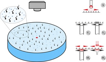
The experiments were performed in a cylindrical glass cuvette filled with high-purity water (figure 1). A few cuvettes with different diameters (from 8 to 17 cm) were used. The water layer depth was varied from 1 to 4 cm. An axisymmetric flow was generated by a localized source located at the axis of the cuvette. A few types of sources, which differ in the driving force setting the fluid in motion, were applied: surface type (S), volume type (V) and mixed type (M) sources. In the first case, the fluid motion was initially generated at the interface due to the solutal Marangoni mechanism only, and the fluid motion in the volume was induced by viscous coupling between interface and subphase. To this end, an acetone droplet a few millimetres in size (see source S in figure 1), pendant at the end of a thin needle and located near the water surface, was utilized as the S source. Acetone vapour, being denser than the ambient air, settled onto the water surface, lowering the surface tension at the centre. This gives rise to the solutal Marangoni tangential stress, which drives the fluid at the interface towards the periphery of the cuvette.
The sketch of the cuvette and the design of the sources of different type.

In the case of the V source, fluid motion was generated solely in the volume, and the interface was then entrained due to viscous forces. For this purpose, pure water was fed through a thin stainless steel tube (1 mm in external diameter) installed from the side of the fluid perpendicular to the interface (see source  ${\rm V}_1$ in figure 1). The distance from the upper tube face to the liquid surface was
 $60\pm 20\ \mathrm {\mu }{\rm m}$. The radial spreading of the fluid led to the formation of an axisymmetric flow in the volume. Special attention was paid to the surface quality of the tube upper face, as well as to the absence of inclination in relation to the water surface; analysis was performed using optical methods. Such a design allowed the water surface over the source to remain free. However, it can be used only at a relatively low rate of the flow passing through the tube (
 $q<0.13\ {\rm g}\ {\rm s}^{-1}$), when the surface deformation over the source is small. At higher flow rates (
 $q<1.6\ {\rm g}\ {\rm s}^{-1}$), the source of another design was applied (see source
 ${\rm V}_2$ in figure 1). A thin flat disk with diameter of 5 mm was located at the water surface over the vertical tube with an external diameter of 5 mm at a distance of
 $400\pm 20\ \mathrm {\mu }{\rm m}$. The disk and tube were coaxial. The intensity of the flow generated by the V source depends both on the flow rate of the fluid passing through the tube and on the gap between the tube face and the disk (
 ${\rm V}_2$), or the water surface (
 ${\rm V}_1$).
In the case of the M source, the fluid motion was generated at the interface and in the volume. Two types of M source, which differed in their flow generation mechanisms, were used. In the first case, the design of the source was the same as  ${\rm V}_1$. The only difference was that an aqueous solution of ethanol (up to 10 % mass concentration) was fed through a thin stainless steel tube instead of pure water (see the source
 ${\rm M}_1$ in figure 1). Falling onto the interface, the ethanol lowered the surface tension at the centre, thus leading to the appearance of a radially directed tangential stress due to the solutal Marangoni mechanism. At the same time, the flow rate of the fluid passing through the tube provides the radial flow in the volume as in the case of the V source. The advantage of this source is that it allows for the generation of the most intense flow, while having good azimuthal uniformity. The thermocapillary mechanism was used to induce the fluid motion in the case of the second of the M sources (see source
 ${\rm M}_2$ in figure 1). To this end, an image of the filament of a halogen lamp was projected onto the water surface, forming there a thermal spot of approximately 5 mm in size. The water surface temperature within the spot was regulated by changing the power of the electric current through the lamp (
 $0< P<100$ W). This gave rise to a centrifugal fluid motion at the interface due to the thermal Marangoni mechanism. Since some part of the incident radiation is absorbed under the interface, thermogravitational convection inevitably develops in the volume. A key advantage of this source is that it allows one to measure the temperature distribution at the interface and to control the value of the tangential stress caused by the thermocapillary mechanism.
2.2. Visualization techniques
A small number of light-scattering particles (silver-coated hollow glass spheres with average size of  $15\ \mathrm {\mu }{\rm m}$, Dantec) of neutral buoyancy were added to the water to visualize the flow structure in the volume and at the interface. Before use, the particles passed a multi-stage cleaning procedure, involving consecutive washing in acetone, isopropanol and high-purity water, to prevent uncontrolled impurities from entering the water. The motion of the particles in the plane of a thin light sheet, formed by laser emission, was recorded with a video camera with a high spatio-temporal resolution and transferred to a PC for further processing. We used two video cameras, of which one is a VIDEOSCAN camera with 11 megapixel Kodak matrix (KAI-11002) and 0.3 f.p.s., and another is a IDS UI-3250ML with 2 megapixel resolution and 60 f.p.s. To visualize the flow structures only on the water surface, a small amount of talc, preliminarily kept within 1 h at a temperature 700 K to remove uncontrolled organic impurities, was applied to it.
An FLIR SC5000 video camera with a matrix sensitive in the infrared range ( $2.5\text {--}5.0 \ \mathrm {\mu }{\rm m}$, matrix resolution
 $320\times 256$ pixels, sensitivity 20 mK) was used to measure temperature at the water surface (
 ${\rm M}_2$ source). The video was transferred to a PC, where it was processed using the standard FLIR software, which yielded the temporal and spatial distributions of both differential and integral temperature characteristics.
2.3. Water surface cleaning technique and application of a surfactant layer
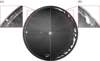
Prior to each experiment, the cuvette and all the components, which are in contact with water during the test, were thoroughly cleaned and rinsed with high-purity water. Then, the cuvette was filled with the high-purity water and the interface was finally cleaned with an aspirator to remove possible residual impurities. The criterion for a clean interface, free of any impurities, was the development of an axisymmetric flow in the entire cuvette, irrespective of the source type inducing it (see the left half of the image in figure 2). When there are residual impurities on the water surface, a system of small-scale vortices forms at the surface periphery (see right half of the image in figure 2). In this case, the experiment was interrupted, and additional cleaning of the water surface was performed.
The flow structure observed on a clean water surface (a), and on a water surface containing a small amount of residual impurities (b), exposure time  $t_{exp}=1\ {\rm s}$.

Directly before the experiment started, a layer of insoluble surfactant, namely oleic acid, of known surface concentration was applied to the clean water surface. The surface pressure isotherm of oleic acid, i.e. the dependence of surface pressure  ${\rm \pi} ={{\sigma }_{0}}-{\sigma }_{f}$ on the relative surface concentration
 $\varGamma /\varGamma _e$ at a fixed temperature is presented in figure 3. Here,
 ${\sigma }_{0}$ is the surface tension of pure water,
 ${{\sigma }_{f}}$ is the surface tension of the water surface with a surfactant film,
 $\varGamma _e=7.2\times 10^{-10}\ {\rm mol}\ {\rm cm}^{-2}$ is the surface concentration corresponding to the saturated monolayer (Abramzon & Gaevoy Reference Abramzon and Gaevoy1979). In the range of surface pressures available in the experiments the isotherm has a relatively simple form consisting of two linear sections which correspond to different phase states of the surfactant in the layer (Adam Reference Adam1952; Adamson & Gast Reference Adamson and Gast1967; Shmyrov et al. Reference Shmyrov, Mizev, Demin, Petukhov and Bratsun2018). The initial part of the curve in the concentration range
 $\varGamma /\varGamma _e<0.38$ corresponds to the gaseous phase state and is characterized by high compressibility
 ${\rm d}{\rm \pi} /{\rm d}(\varGamma /\varGamma _e)\approx 0.5\ {\rm dyn}\ {\rm cm}^{-1}$. At higher concentration
 $\varGamma /\varGamma _e>0.38$, the oleic acid molecules are in the liquid-expanded phase state, which has much lower compressibility
 ${\rm d}{\rm \pi} /{\rm d}(\varGamma /\varGamma _e)\approx 15\ {\rm dyn}\ {\rm cm}^{-1}$. In some experiments we used a stearic acid as a surfactant. This substance is also insoluble in water and has a similar form of the isotherm (see figure 3). In comparison with oleic acid, the isotherm of stearic acid has a longer part corresponding to the gaseous phase state
 $\varGamma /\varGamma _e<0.7$ (
 $\varGamma _e=7.9\times 10^{-10}\ {\rm mol} \ {\rm cm}^{-2}$ for stearic acid). The surfactants were preliminarily dissolved in n-hexane in the volume ratio of 1 : 1000. A small amount (few microlitres) of the solution was deposited on the clean water surface. After complete evaporation of the n-hexane, the film of surfactant molecules with a given surface concentration remained at the interface.
Surface pressure  ${\rm \pi}$ for oleic (1 and 2) and stearic (3) acids as a function of a relative surface concentration
 $\varGamma /\varGamma _e$ (
 $\varGamma _e$ stands for the saturated monolayer concentration). The symbols indicate: 1, our results, 2,3, the data taken from Abramzon & Gaevoy (Reference Abramzon and Gaevoy1979).

3. Experimental results
3.1. General overview of the flow structures
Analysis of the experimental results shows that, as soon as the source is switched on, one of two main scenarios for convective motion evolution occurs, regardless of the type of source. As in the two-dimensional case studied by us earlier, the convective flow structure is determined, first of all, by the ratio of two opposite tangential stresses induced at the interface by the source and the compressed surfactant film. If the shear stress generated by the source at the centre exceeds the surface pressure from the surfactant layer side, then a centrifugal flow develops at the interface. One to two seconds later, the flow at the periphery damps, yet in the central part it remains intense. As a result, an annular boundary of radius  ${{r}_{c}}$, separating the two zones, is formed on the surface. An axisymmetric intense fluid flow with a characteristic velocity of approximately
 $10\ {\rm cm}\ {\rm s}^{-1}$ remains in the inner zone. In the outer zone, a slow multi-vortex flow, periodic in the azimuthal direction and having a characteristic velocity of approximately
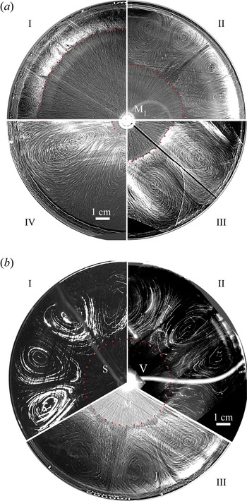
 $0.1\ {\rm cm}\ {\rm s}^{-1}$, develops a few seconds later (see figure 4 and Movie 1 in the supplementary material available at https://doi.org/10.1017/jfm.2022.205). Generation of the central zone and the dependence of its size on the control parameters of the problem will be discussed in detail in §§ 3.2 and 3.3.
(a) The flow structure, observed at the interface, in experiments with  ${\rm M}_1$ type source under the following experimental conditions: I –
 $q=0.021\ {\rm g}\ {\rm s}^{-1}$,
 $C=10\,\%$,
 $\varGamma /\varGamma _e=0.075$, exposure time
 $t_{exp}=0.8\ {\rm s}$, II –
 $q=0.005\ {\rm g}\ {\rm s}^{-1}$,
 $C=5\,\%$,
 $\varGamma /\varGamma _e=0.075$,
 $t_{exp}=1.7 \ {\rm s}$, III –
 $q=0.023\ {\rm g}\ {\rm s}^{-1}$,
 $C=2.5\,\%$,
 $\varGamma /\varGamma _e=0.23$,
 $t_{exp}=0.8\ {\rm s}$, IV –
 $q=0.036\ {\rm g}\ {\rm s}^{-1}$,
 $C=10\,\%$,
 $\varGamma /\varGamma _e=0.45$,
 $t_{exp}=0.5\ {\rm s}$. (b) The flow structure, observed at the interface, in experiments with various types of source: I – S type,
 $d=1.8$ mm,
 $h=1.5$ mm,
 $\varGamma /\varGamma _e=0.35$,
 $t_{exp}=7\ {\rm s}$, II –
 ${\rm V}_2$ type,
 $q=1.27\ {\rm g}\ {\rm s}^{-1}$,
 $\varGamma /\varGamma _e=0.35$,
 $t_{exp}=3\ {\rm s}$, III –
 ${\rm M}_1$ type,
 $q=0.0021\ {\rm g}\ {\rm s}^{-1}$,
 $C=5\,\%$,
 $\varGamma /\varGamma _e=0.23$,
 $t_{exp}=4\ {\rm s}$.

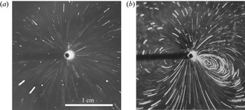
The second of these scenarios has been observed at a relatively low source intensity, i.e. when the shear stresses caused by the source at the centre do not exceed the surface pressure from the surfactant layer side. In this case, the central zone does not ever appear and the flow structure, which occurs after a source has been switched on, essentially depends on the source type and its intensity. The fluid remains always motionless both at the interface and in the volume for the S type source. When using the V and M sources, an axisymmetric radial flow develops in the volume beneath the interface at low enough source intensity (see figure 5a). The interface is motionless in this case. When analysing the image it is necessary to take into account the finite thickness of the light sheet, which results in tracks of different lengths. The zero length tracks correspond to the particles at the interface, whereas the tracks drawn by the particles in the volume have different lengths depending on the depth. At higher intensity, a multi-vortex flow appears in the vicinity of the source both at the interface and in the volume (see figure 5(b) and supplementary movie 2). The vortex centres are located close to the source, where the characteristic flow velocity on the surface is of the order of  $0.1\ {\rm cm}\ {\rm s}^{-1}$. The vortices become larger in size, gradually taking up the entire area of the interface as the source intensity increases. The structure of this type of flow and its evolution when changing the intensity of the source and the characteristics of the surfactant layer will be discussed in more detail in § 3.5. It is worth noting that the above described flow patterns are formed during a short transient period (a few seconds) and then they remain stationary under fixed conditions of the experiment.
The flow structure, observed at the interface and beneath, in experiments with the  ${\rm V}_1$ type source under the following experimental conditions (a)
 $q=0.005\ {\rm g}\ {\rm s}^{-1}$,
 $\varGamma /\varGamma _e=0.5$,
 $t_{exp}=9\ {\rm s}$; (b)
 $q=0.017\ {\rm g}\ {\rm s}^{-1}$,
 $\varGamma /\varGamma _e=0.5$,
 $t_{exp}=3\ {\rm s}$.

As will be shown below, the problems related to the formation of an inner zone with an intense axisymmetric flow and the appearance of a multi-vortex structure in the stagnant zone have different physical causes and should be analysed independently. First, we consider the formation of a two-zone flow structure.
3.2. The conditions for establishing a stationary state
It is evident that the formation of a two-zone flow structure is caused, as in the two-dimensional case, by the displacement of the surfactant from the centre to the periphery, where it forms a stagnant zone. By changing the source intensity and surfactant concentration, it is possible to change the position of the boundary between the zones, which hereafter we refer to as a stagnant line. Figure 4(a) presents a series of photographs showing the flow pattern at the interface for different values of the source power and surfactant concentration. It is seen that a decrease in the source intensity or an increase in the surfactant amount at the interface leads to a decrease in the radius of the inner zone. In this case, the size of the vortices within the stagnant zone increases, and their number, decreases.
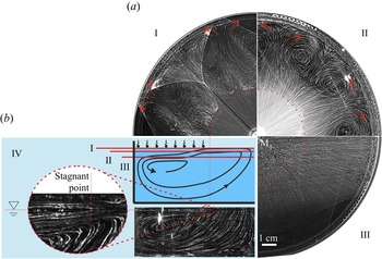
Figure 4(b) presents photographs of the convective flow pattern observed at the interface for the three different types of source: S (sector I), V $_2$ (sector II) and M
 $_1$ (sector III). For clarity, the parameters are selected so that the size of the inner zone is the same in all cases. Two images without radial traces in the inner zone (two upper sectors in figure 4b) correspond to the experiments in which tracers (talc particles) were applied only to the water surface. It is clearly seen that the flow pattern is similar for the different types of source, independently of the way the flow was induced, which indicates the same basic mechanisms behind the flow formation. The stationary flow structure and, therefore, the stationary position of the stagnant line are governed by a balance between the shear stresses applied on the interface on the part of both the source and the surfactant layer. The contribution of the latter is determined by the value of the surface pressure, which can be obtained from the surface pressure isotherm
 ${\rm \pi} (\varGamma )$ which is unique for each surfactant. On the part of the source, the interface is affected by a counter-stress the nature of which depends on the type of source. It can be either the stress of solutocapillary origin in the case of the S type source or viscous traction acting upon the interface in the case of a bulk source. For mixed sources, the contribution of both mechanisms should be taken into account.
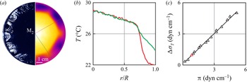
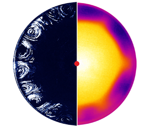
The balance between the shear stresses acting on the interface can be quantitatively demonstrated in the case of the M $_2$ source. Note that a shear stress itself is a local characteristic demonstrating the action of a force at each point on the interface. At the same time, in experiments we usually deal with integral characteristics, which reflect a summary action of the forces over the entire interface. Such an integral characteristic in the situation under consideration, is the increment of surface tension caused by both the thermocapillary and solutocapillary mechanisms. A convective flow pattern on the surface and an infrared image of the surface obtained for the
 ${\rm M}_2$ source are presented in figure 6. As one can see, both visualization techniques are able to adequately reproduce the multi-vortex flow structure within the stagnant zone. The temperature profile measured in a radial direction (figure 6b) shows that the main part of the temperature drop accounts for the stagnant zone, whereas the temperature changes only slightly in the inner zone. This is caused by intensive heat transfer due to thermocapillary convection. The temperature difference measured at the interface can be used to calculate the surface tension increment due to thermocapillary mechanism
 $\Delta {{\sigma }_{T}}={{{\sigma }'}_{T}}\,\Delta T$ (here
 ${{{\sigma }'}_{T}}=0.17\ {\rm dyn}\ ({\rm cm}\ {\rm K})^{-1}$ is the thermal coefficient of surface tension (Vargaftik, Volkov & Voljak Reference Vargaftik, Volkov and Voljak1983) and
 $\Delta T$ is the temperature difference measured at the interface within the stagnant zone). For the experiment presented in figures 6(a) and 6(b) the temperature difference
 $\Delta T=5.5\,K$ which gives
 $\Delta {{\sigma }_{T}}\approx 0.94\ {\rm dyn}\ {\rm cm}^{-1}$. Together with the thermocapillary force one needs to take into account the viscous force acting on the part of the flow spreading beneath the stagnant zone. The contribution of the viscous stress (per unit length along the stagnant line) can be roughly estimated as
 $\tau ={\eta \Delta vL}/{\delta }$, where
 $\eta$ is the dynamic viscosity of water,
 $\Delta v$ is the change in the radial velocity in a near-surface layer of thickness
 $\delta$ and
 $L$ is the radial size of the stagnant zone. In the case of quite intense thermocapillary flow
 $\Delta v$ can reach
 $2\text {--}3\ {\rm mm}\ {\rm s}^{-1}$ at depth
 $1\ {\rm mm}$, which gives us
 $\tau \sim {{10}^{-2}}\ {\rm dyn}\ {\rm cm}^{-1}$ at
 $L\sim {{10}^{0}}\ {\rm cm}$. Note that the above value calculated by the maximum velocity is overestimated and the real contribution of the viscous forces should be even less. One can see that, to a first approximation, the contribution of the viscous stress can be neglected in contrast to the thermocapillary one. The surface pressure within the stagnant zone, which is the surface tension increment caused by the solutocapillary mechanism, can be found from the surface pressure isotherm
 ${\rm \pi} (\varGamma )$ for the surfactant concentration in the compressed layer. The latter can be determined by applying the law of conservation of the amount of insoluble surfactant at the interface
 $\varGamma ={\varGamma }_{0}/(1-{{({{{r}_{c}}}/{R})}^{2}})$, where
 ${{\varGamma }_{0}}$ is the initial surface surfactant concentration in the unperturbed layer,
 ${{r}_{c}}$ is the radius of the stagnant line and
 $R$ is the cuvette radius. At
 ${{\varGamma }_{0}}=0.19{{\varGamma }_{e}}$ and
 ${{{r}_{c}}}/{R}=0.73$, which corresponds to the experiment presented in figure 6(a), the surface pressure is equal to
 ${\rm \pi} \approx 0.9\ {\rm dyn}\ {\rm cm}^{-1}$.
(a) The flow structure, being visualized at the interface with talcum tracers (left half),  $t_{exp}=10\ {\rm s}$, and the infrared image of the interface (right half), obtained in the experiment with the
 ${\rm M}_2$ type source,
 $P=80\ {\rm W}$,
 $\varGamma /\varGamma _e=0.19$. (b) The temperature profiles measured in two radial directions marked in figure 6(a). (c) Surface tension increment caused by thermocapillary mechanism vs surface pressure in compressed surfactant layer. Red triangle denotes the conditions for the experiment, presented in figure 6(a).

The values of the shear stresses calculated above are shown on the graph of surface tension increment caused by the thermocapillary mechanism vs surface pressure in a compressed surfactant layer (see figure 6c, red colour symbol). The results obtained in other experiments with the  ${\rm M}_2$ type source are also presented on the same graph. It is seen from figure 6(c) that these two quantities are always equal each other, which indicates the balance between the shear stresses in a stationary state. This fact may seem trivial at first glance, but direct experimental measurements showing the shear stress balance under conditions of a fully developed flow are performed for the first time.
3.3. Elasticity number and stagnant line position
The above results show that, for successful prognosis of the experimental conditions at which the inner zone with a radial flow can occur, the surface pressure in the initial surfactant layer must be compared with the magnitude of the shear stress acting on the interface directly nearby the source. The ratio of these two quantities is known as the elasticity number, the non-dimensional parameter which was first introduced in Homsy & Meiburg (Reference Homsy and Meiburg1984) for the case of thermocapillary convection. When the elasticity number becomes less than unity, the surfactant layer shifts away from the centre under the action of a source, and a two-zone flow structure appears. The lower the elasticity number, the more the stagnant line shifts towards the periphery (see figure 4a). In our previous studies (Shmyrov et al. Reference Shmyrov, Mizev, Demin, Petukhov and Bratsun2018, Reference Shmyrov, Mizev, Demin, Petukhov and Bratsun2019) on a two-dimensional case, it was shown that the position of the stagnant point can be determined by the value of the elasticity number.
In this context, this parameter can also be introduced to describe the inner zone formation and stagnant line position. The numerator of this parameter is the surface pressure at the initial surface concentration  ${\rm \pi} ({{\varGamma }_{0}})$, which can be taken from the surface pressure isotherm for a particular surfactant. The expression for the denominator depends on the way the flow is generated, and it will vary for different sources. If we neglect the influence of thermogravitational convection in the case of M
 $_2$ source, then the elasticity number can be expressed as follows:
 \begin{equation} E=\frac{{\rm \pi} \left( {{\varGamma }_{0}} \right)}{\Delta {{\sigma }_{T}}}. \end{equation}
For the V type source, the denominator is equal to the magnitude of the viscous shear stress  $\tau$ (per unit length along the source edge) applied to the interface from the side of the spreading fluid flow directly near the source
 \begin{equation} E=\frac{{\rm \pi} \left( {{\varGamma }_{0}} \right)}{\tau }. \end{equation}
Assuming that, for the slit gap between the upper tube face and the interface (or the disk in the case of the  ${\rm V}_2$ source), the velocity profile is described by the Poiseuille law, the magnitude of the shear stress can be expressed as
 ${\tau }={3\eta q}/2{\rm \pi} \rho {{H}^{2}}$, where
 $H$ is the gap thickness,
 ${\eta }$ and
 ${\rho }$ are the viscosity and density of water and
 $q$ is the mass flow rate of the liquid through the source.
When calculating the denominator in the case of the  ${\rm M}_1$ source, it is necessary to take into account the contribution of both the surface mechanism of solutocapillary origin and the volumetric mechanism due to the viscous entrainment of the interface
 \begin{equation} E=\frac{{\rm \pi} \left( {{\varGamma }_{0}} \right)}{\Delta {{\sigma }_{c}}+\tau }, \end{equation}
where  $\Delta {\sigma }_{c}={{{\sigma }'}_{c}C}$ is the change in the surface tension of water when an ethyl alcohol solution of concentration
 $C$ is added to it, and
 ${\sigma }'_{c}$ is the concentration coefficient of surface tension.
Under the conditions prevailing in this study, the dependence of the stagnant line position on the elasticity number would be expected as  ${r}_{c}/{R}=1-{{E}^{n}}$. Indeed, the form of the function should satisfy the following requirements: at
 $E\to 1$,
 ${{r}_{c}}\to 0$, and at
 $E\to 0$,
 ${{r}_{c}}\to R$. Strictly speaking, at
 $E\to 1$, the size of the stagnant zone must tend to the size of the source
 ${{r}_{s}}$. However, given that
 ${{r}_{s}}\ll R$, this correction can be neglected to a first approximation. Figure 7(a) illustrates the dependence of
 $1-{{{r}_{c}}}/{R}\;$ on the elasticity number for three types of source. The value of the elasticity number is calculated by formulas (3.1)–(3.3). There are no data concerning the experiments with an S type source in figure 7(a), since the expression for the denominator of the elasticity number is hard to connect with experimental parameters. Experimental observations have shown that the larger the acetone droplet size and the closer it is to the water surface, the higher the S type source intensity. However, since there is no way to measure the concentration of the acetone molecules adsorbed on the water surface, calculation of the surface tension increment caused by solutocapillary mechanism turns out to be impossible.
(a) The dependence of the non-dimensional stagnant zone size on the elasticity number for different types of source. (b) parameter  $\xi$ defined by (3.4) vs elasticity number for different types of source. The dotted curve is plotted using (3.4). (c) The azimuthal wavenumber of the multi-vortex structure as a function of the non-dimensional position of the stagnant line for different types of source. Using (3.5), the curves are plotted for
 $m=1$ (red solid line) and
 $m=2$ (red dotted line). The symbols in all graphs indicate different types of source: black triangles, M
 $_1$; red squares, M
 $_2$; blue circles,
 ${\rm V}_2$; green diamonds, S.

The first thing that draws attention when analysing figure 7(a) is the fact that, for all dependencies, the size of the central zone tends to zero as the elasticity number goes to unity. This shows that the elasticity number allows us to predict the moment of formation of the inner zone, regardless of the type of source. In the range of  $0< E<1$ the data corresponding to various sources form different dependencies. Moreover, the data describing the experiments with the
 ${\rm M}_1$ source form two separate groups essentially differing in slope. It should be noted here that the source
 ${\rm M}_1$ is the only one that has enough power to operate with the layers in the liquid-expanded phase state. Analysis of the experimental data shows that the left group of data refers to the experiments in which the surfactant has been initially in the gaseous phase within the stagnant zone. The right group corresponds to the case when the surfactant was in the liquid-expanded phase state from the very beginning. Unlike the
 ${\rm M}_1$ source, the
 ${\rm M}_2$ and
 ${\rm V}_2$ sources are not intense enough to manipulate the surfactant layers in the liquid-expanded phase state. Both dependencies plotted for these sources (curves 2 and 3 in figure 7a) correspond to the gaseous phase state or to the very beginning of the liquid-expanded one.
A similar situation was observed in the two-dimensional case we studied earlier (Shmyrov et al. Reference Shmyrov, Mizev, Demin, Petukhov and Bratsun2019). The experimental data plotted in the coordinates  ${{{x}_{c}}}/{L}=f(E)$ formed a single dependence
 ${{{x}_{c}}}/{L}=1-E$ only if the surfactant layer remained in the gaseous phase state. If a phase transition occurred on parts of the layer, then the data formed a different dependence. As a result, a family of curves arose, each of which corresponded to a certain initial surface concentration. Thus, for a certain
 $E$, it was possible to obtain different values of the stagnant point position in the experiment, depending on the initial concentration of the surfactant. In the same way, in the situation shown in figure 7(a), the data group on the left side of the graph corresponds to the experiments with different initial concentrations and, therefore, the points relate to different curves. The reason is that the elasticity number is defined in terms of the initial concentration of the surfactant and the power of the source in the centre of the cuvette. This allows prediction of the formation of the two-zone flow structure at
 $E=1$. However, in order to find the position of the boundary between the zones at
 $E<1$, it is necessary to know a concentration in a squeezed surfactant layer and a flow intensity at some distance from the source.
Therefore, we believe that the representation of the experimental data in the coordinates  $1-{{{r}_{c}}}/{R}=f(E)$ is not convenient, because in this case the position of the stagnant line can be unambiguously described only under a fixed type and size of source as well as a fixed surfactant used (including its phase state). Changing any of these parameters will change the dependence. This is inconvenient for a researcher and has no predictive power. A detailed description of the problem and the selection of relevant dimensionless parameters requires a broad theoretical study, including analysis of the heat and mass transfer processes both in the volume and on the surface of the liquid. The position of the boundary between the two zones can be determined by the integral balance of the counter-shear stresses of both capillary and viscous natures, distributed in a complex way along the radial coordinate.
Nevertheless, the data obtained in different experiments can be described in a unified way within the framework of a simplified model of interaction between the flow and the surfactant layer. Let assume that this interaction takes place within the narrow zone near the stagnant line, rather than along the entire stagnant zone surface. This means that the surfactant concentration is constant over the stagnant zone except for the area near the stagnant line. This holds true for small enough sizes of the inner zone. In this case, the effect of the source on the surfactant layer at the distance  ${{r}_{c}}$ can be represented as
 $I={{{I}_{0}}}/{{({{r}_{c}}}/{{{r}_{0}}{{)}^{n}}}}$,
 ${{r}_{c}}\in ( {{r}_{0}},R )$, where
 ${{I}_{0}}$ is the source intensity at a distance equal to its size
 ${{r}_{0}}$. The exponent
 $n$ indicates how fast the intensity decays in a radial direction. The action on the part of the surfactant layer can be expressed in terms of the surface pressure in the compressed layer as
 ${\rm \pi} ={{{{\rm \pi} }_{0}}}/{1-{{( {{{r}_{c}}}/{R})}^{2}}}$. Taking into account that
 $I={\rm \pi}$ in a stationary state and that
 $E\equiv {{{{\rm \pi} }_{0}}}/{{{I}_{0}}}$, we obtain the following relation between the elasticity number and the geometrical parameters of the problem:
 \begin{equation} E=\frac{1-{{\left( {{{r}_{c}}}/{R}\right)}^{2}}}{{{\left( {{{r}_{c}}}/{{{r}_{0}}} \right)}^{n}}}\equiv \xi. \end{equation}
Figure 7(b) presents the experimental results in coordinates  $\xi (E)$ and the curve plotted according to (3.4). When calculating the value of
 $\xi$, the actual sizes of the sources were used (see § 2). The exponent
 $n=1$ was taken for all types of source. This choice of the exponent is physically justified since the radial velocity in cylindrical coordinates should decay as
 ${{r}^{-1}}$. In the case of
 ${\rm V}_2$, the flow represents the radial jet, the solution for which was derived by Squire (Squire Reference Squire1955). For the heat source, such a decay law was demonstrated in Bratukhin & Maurin (Reference Bratukhin and Maurin1967). In the case of the
 ${\rm M}_1$ source, the flow is generated mainly by the solutal Marangoni mechanism. This kind of flow has been studied recently by Bandi et al. (Reference Bandi, Akella, Singh, Singh and Mandre2017) and Mandre (Reference Mandre2017). It was shown that the radial velocity can decay with the radial distance at different rates depending on the sorption kinetics. If the surfactant exchange between the surface and the volume occurs much faster than the hydrodynamic time scale, then the radial velocity decays as
 ${{r}^{-1}}$. With the inverse ratio of these characteristic times, the decay is as
 ${{r}^{-{3}/{5}}}$. Taking into account the rather fast sorption kinetics of ethanol, the choice of
 $n=1$ seems valid.
It is seen from figure 7(b) that the data obtained for various sources form a unified dependence which is well described by (3.4) in the range  $0.1<\xi <1$, which corresponds to the small sizes of the inner zone with
 ${{{r}_{c}}}/{R}<0.3$. This agreement is worse in the range of smaller
 $\xi$, where the above assumption is invalid for narrow enough stagnant zones.
3.4. Surface flow structure within a stagnant zone at  $E<1$

Analysis of the vortex structure formed at the interface within the stagnant zone has revealed that the size and number of the vortices are independent of the type and intensity of the source and the surface pressure in the surfactant layer and determined only by the width of the stagnant zone. In other words, when the position of the stagnant line is fixed, the multi-vortex structure is the same for all types of source (see e.g. figure 4b). Figure 7(c) shows the dependence of the azimuthal wavenumber  ${{k}_{\varphi }}={2{\rm \pi} }/{{{\lambda }_{\varphi }}}$ (where
 ${{\lambda }_{\varphi }}$ is the wavelength of the structure in the azimuthal direction measured in radians), which is numerically equal to half the number of vortices, on the dimensionless position of the stagnant line. It is seen that, regardless of the type of source, its intensity and the initial surface concentration of surfactant, all experimental data form a single dependence, which can be described by the following equation:
 \begin{equation} {{k}_{\varphi }}=\frac{{\rm \pi} m\left( 1+{{{r}_{c}}}/{R}\right)}{2(1-{{{r}_{c}}}/{R})}, \end{equation}
where  $m={{{l}_{r}}}/{{{l}_{\varphi }}}$ is the ratio of the radial and azimuthal dimensions of a single vortex. Equation (3.5) was derived provided that an integer number of vortex pairs, the radial size of which is equal to the width of the stagnant zone, completely fills the stagnant zone (as shown in the sketch in figure 7c). It can be seen that, at small sizes of the convective zone, the experimental results are better described by the curve with
 $m=2$ (red dotted line in figure 7c), which corresponds to the vortices elongated in the radial direction. For the narrow stagnant zone, the best approximation for the given data is obtained at
 $m=1$ (red solid line in figure 7c). In our opinion, such a change in the geometry of the vortex structure can be associated with the transition from a cylindrical to a planar geometry. Indeed, since the radial velocity decays as
 $1/r$, the main changes of the viscous stress beneath the stagnant zone occur closer to the centre. In the case of a wide stagnant zone, when
 ${r_c}/R$ is small enough, the viscous stress beneath the surfactant layer varies essentially between the stagnant line and the cuvette side boundary and the impact of the cylindrical geometry is profound. The vortices in this case are elongated in the radial direction and their centres are shifted closer to the stagnant line (see figure 4a, IV). If
 ${r_c}/R>0.6$, the stagnant zone turns out far from the source and the variations of the viscous stress within the limits of the stagnant zone become small enough to consider the geometry as planar to a first approximation. This transition results in more symmetric vortices.
At the end of this section it is worth discussing the spread in data which is clearly visible in figure 7(c) and corresponds to the experiments with the  ${\rm M}_1$ source. The reason for this is the ethanol which is used to produce the solutocapillary flow. The ethanol itself is a surfactant, although not a classical one. It demonstrates surface-active properties on the water surface. Being accumulated in the volume and at the interface, it is able to change in part the surface-active properties of the insoluble surfactant, thus varying the conditions of the experiment. This influence should depend on both the ethanol concentration and the experiment duration. Unfortunately, this factor cannot be avoided or taken in some way into account. The impact of ethanol manifests itself not only in the data spread but also in the shape of vortices. The centres of the vortices formed in the case of the
 ${\rm M}_1$ source are always shifted a little closer to the stagnant zone periphery (see, for example the corresponding images in figure 4), whereas the centres of the vortices are located symmetrically with respect to the stagnant zone for all other sources. This results in a greater quantity of vortices in comparison with other sources at a fixed size of the stagnant zone. This fact is illustrated in figure 7(c).
3.5. Surface flow structure within a stagnant zone at $E\geqslant 1$

At  $E\geqslant 1$, the inner zone is not formed, and the entire surface is a stagnant zone. However, a flow can appear both at the interface and in the volume depending on the type of source used. In the case of the S type source, the fluid at the interface and in the volume is always motionless under
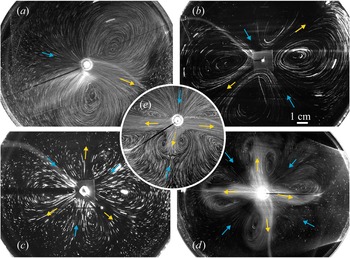
 $E\geqslant 1$. When using the sources of V or M type, which can generate a flow in the fluid volume, a slow axisymmetric flow develops beneath the interface under very low source intensities. This was mentioned in § 3.1 (see figure 5a). At the same time, the interface remains motionless. As the source intensity increases, a multi-vortex flow similar to that described above is formed at the interface (figure 8). However, in the case of
 $E\geqslant 1$, the number of vortices depends on the source intensity. At low intensity, a two-vortex flow is formed at the interface (see figures 8a and 9a). As intensity increases, the number of vortices increases up to four (figure 8b), six (figure 8c) and eight (figure 8d) vortices. The maximum number of vortices (without the formation of an inner zone) observed during the experiments is ten. Restructuring of the flow at the interface under an increase of source intensity occurs due to the formation of a new centrifugal jet in the vicinity of the source, which spreads towards a centripetal flow (figure 8e). It is important to note here that the vortex structure with
 ${{k}_{\varphi }}>1$ was observed at both
 $E<1$ and
 $E\geqslant 1$, and the flow with
 ${{k}_{\varphi }}=1$ (two-vortex flow structure) was found at
 $E\geqslant 1$ only. The flow structures presented in figure 8 remain stable over time, at least, for a few minutes, which is typical of a single experiment. The transitions between the flow regimes corresponding to a different number of vortices are reversible when the source intensity changes back.
The surface flow structure for  $E\geqslant 1$. (a)
 $k_\phi =1$, the source of
 ${\rm M}_1$ type:
 $q=0.003\ {\rm g}\ {\rm s}^{-1}$,
 $C=2.5\,\%$,
 $\varGamma /\varGamma _e=0.375$,
 $t_{exp}=3.2\ {\rm s}$. (b)
 $k_\phi =2$, the source of
 ${\rm V}_1$ type:
 $q=0.13\ {\rm g}\ {\rm s}^{-1}$,
 $\varGamma /\varGamma _e=0.43$,
 $t_{exp}=7\ {\rm s}$. (c)
 $k_\phi =3$, the source of V2 type:
 $q=0.19\ {\rm g}\ {\rm s}^{-1}$,
 $\varGamma /\varGamma _e=0.18$,
 $t_{exp}=7\ {\rm s}$. (d)
 $k_\phi =4$, the source of
 ${\rm M}_1$ type:
 $q=0.017\ {\rm g}\ {\rm s}^{-1}$,
 $C=1.5\,\%$,
 $\varGamma /\varGamma _e=0.15$,
 $t_{exp}=4\ {\rm s}$. (e)
 $k_\phi =2$, transition to
 $k _\phi =3$, the source of
 ${\rm M}_1$ type:
 $q=0.011\ {\rm g}\ {\rm s}^{-1}$,
 $C=2.5\,\%$,
 $\varGamma /\varGamma _e=0.2$,
 $t_{exp}=3.2\ {\rm s}$.

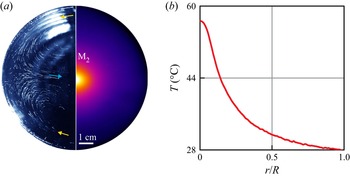
(a) The flow structure, being visualized at the interface with tracers (left half), and the infrared image of the interface (right half), both obtained in the same experiment with the  ${\rm M}_2$ type source for the case of
 $E\geqslant 1$:
 $k_\phi =1$,
 $P=90\ {\rm W}$,
 $\varGamma /\varGamma _e=0.55$,
 $t_{exp}=15\ {\rm s}$. (b) The temperature profile measured in a radial direction.

In the case of the  ${\rm M}_2$ source, the temperature distribution on the surface (see figure 9a) is described by a smooth function (see figure 9b). There is no break of the temperature profile similar to that clearly visible in figure 6(b), which indicates the absence of the inner zone with intense convection. The vortex motion is rather slow in leaving a noticeable trace in the temperature field (for comparison, see figure 6). Since the thermocapillary convection is suppressed by the solutocapillary mechanism at
 $E\geqslant 1$, the thermogravitational mechanism remains the only one that is responsible for the vortex flow development.
It should be emphasized that, at  ${E\geqslant 1}$, the formation of the multi-vortex fluid motion was observed only for some types of source. It has never been detected in the case of the S source. This indicates that the competition of the surface forces alone is insufficient for the appearance of vortices, and a fluid motion in the volume plays the main role in their formation. The motion in the volume always exists for the V and M sources, where the multi-vortex structure is observed at both
 ${E<1}$ and
 ${E\geqslant 1}$. For the S type source, the multi vortex structure develops only at
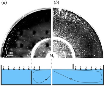
 ${E<1}$, when the radial flow formed in the central part due to the solutocapillary mechanism spreads under the stagnant zone. To trace the role of the volume flow in the formation of the multi-vortex flow, two additional experiments were performed.
In the first experiment, a coaxial annular barrier was inserted into the fluid volume. The height of the barrier was 2–3 mm less than the depth of the fluid layer (figure 10a). This allowed us to limit the existence area of the volume flow to the central zone. At the same time, the surface flow could freely spread up to the cuvette boundary. The elasticity number was chosen so that the radius of the boundary between the zones coincided with the radius of the barrier. In this case, a multi-vortex flow did not develop within the stagnant zone (figure 10a). During the second stage of the experiment, the elasticity number increased due to the reduced source intensity. Therefore, the boundary between the zones shifted towards the centre so that part of the stagnant zone would be inside the area bounded by the barrier. The flow pattern observed in this case is presented in figure 10(a). It is seen that the multi-vortex flow develops on the part of the interface located inside the barrier where the volume flow exists under the stagnant zone. Outside the barrier, where there is no volumetric flow under the surface, the vortices are not formed, regardless of a common interface.
The surface flow structure observed in the experiments with the barrier located in the fluid volume (a)  $q=0.013\ {\rm g}\ {\rm s}^{-1}$,
 $C=5\,\%$,
 $\varGamma /\varGamma _e=0.45$,
 $t_{exp}=7\ {\rm s}$; or in the gas phase (b)
 $q=0.036\ {\rm g}\ {\rm s}^{-1}$,
 $C=5\,\%$,
 $\varGamma /\varGamma _e=0.35$,
 $t_{exp}=0.8\ {\rm s}$.

In the second experiment, a coaxial annular barrier was located on the side of the gas phase touching the fluid surface, thereby dividing the surface into two isolated regions (figure 10b). At the same time, the volumetric flow could freely spread up to the cuvette boundary. The surfactant was applied only to the outer part of the fluid surface. Thus the position of the barrier uniquely determines the location of the boundary between the zones under study. It is seen that the spreading of the volume flow under the stagnation zone leads to the development of a multi-vortex structure.
3.6. Flow structure in the volume
The above experiments have provided evidence that the presence of a flow under the stagnant zone is a necessary condition for the development of a multi-vortex flow pattern. At the same time, the vortices themselves originate at the interface. This finding is supported by the following observations. Figure 11 shows the flow structure observed on the surface and in the volume of fluid, for three horizontal and one vertical planes. Since the experiment was carried out at  ${E<1}$, two zones, separated by the stagnant line of radius
 $r_c$, develop at the interface (see figure 11, sector I). At a depth of 0.5 mm, the centrifugal flow spreads under the stagnation zone, keeping axial symmetry for some distance (see figure 11, sector II). Downstream, the flow divides into separate streams (periodic in the azimuthal direction), which spread up to the cuvette boundary. A pair of counter-rotating vortices forms between the streams. At a depth of 5 mm (figure 11, sector III), the centrifugal flow remains axially symmetric up to the cuvette boundary. Movie 5 in the supplementary materials demonstrates in more detail the flow structure beneath the interface at various depths. The results shown in figure 11 and in movie 5 indicate that the vortices originate at the interface within the stagnant zone where their intensity is maximal. Beneath the surface they quickly damp with depth, giving rise to an axisymmetrical radial flow at depth of approximately 2–3 mm. Thus, the divergent flow generated by the source keeps its axial symmetry far from the interface. The sizes of the vortex structure along the free surface and across differ by at least an order of magnitude.
The flow structure observed in the horizontal planes located at: I – surface,  $t_{exp}=1.5\ {\rm s}$; II – 0.5 mm depth,
 $t_{exp}=5\ {\rm s}$; III – 5 mm depth,
 $t_{exp}=0.8\ {\rm s}$, for the
 ${\rm M}_1$ source:
 $q=0.002\ {\rm g}\ {\rm s}^{-1}$,
 $C=2.5\,\%$,
 $\varGamma /\varGamma _e=0.15$. IV – scheme of the locations of the laser sheet (a) and the flow structure observed in the axial cross-section of a cylindrical cuvette (b).

The structure of the flow in the volume observed in the axial cross-section of a cylindrical cuvette is shown in figure 11, sector IV. Corresponding movies are given in supplementary materials (movies 3 and 4). It is clearly seen that the flow dives under the stagnant zone. Its further motion beneath the stagnant zone leads to the formation of a viscous boundary layer. The videos show the slow motion of the tracers within the stagnant zone. This motion can propagate in the same direction (movie 3) as the flow under the surface or in the opposite direction (movie 4), depending on the azimuthal orientation of the laser sheet relative to the vortices.
3.7. Surfactant properties effect on the formation of the multi-vortex structure
The above experiments were carried out with only one surfactant, namely oleic acid. To study the influence of surfactant properties on the flow structure, we performed the experiments with stearic acid. Both surfactants are fatty acids and have close chemical compositions with an 18-carbon chain, but they are distinct in their molecule structure, which causes the difference in properties (see § 2). The experiments were carried out with the S type source, the intensity of which was fixed. At the same time a surface concentration was selected in such a way as to provide a similar size of the stagnant zone for both surfactants.
The results of the flow visualization at the interface are presented in figure 12. It is seen that the surface within the stagnant zone remains immobile in the case of stearic acid, whereas a multi-vortex structure develops on the surface occupied by oleic acid molecules. In the supplementary materials (movies 6 and 7) there are videos that demonstrate more clearly the difference between these two cases. Taking into account the similar size of the stagnant zones and the same source intensity one can conclude that the same surface pressure is present within both surfactant layers, although it has been obtained at different surface concentrations. The latter fact and the differences in the surface pressure isotherm of the surfactants cause the difference in the elasticity of the layers. However, in contrast to the axisymmetric radial flow, which squeezes the layer, the multi-vortex flow does not disturb the surface concentration, exciting pure shear deformations. Thus, the resistance to a vortex fluid motion arises from viscous stresses alone, regardless of the layer elasticity. Taking into account a fixed volume viscosity, the difference in the surface shear viscosity is the only reason responsible for the difference between the results obtained for the oleic and stearic acid layers. The value of this parameter can vary widely depending on the surfactant forming an adsorbed layer. For most soluble surfactants, the surface shear viscosity is of the order of  $10^{-5}\ {\rm dyn}\ {\rm s}\ {\rm cm}^{-1}$, and
 $10^{-4} \text {--}10^{-3}\ {\rm dyn}\ {\rm s}\ {\rm cm}^{-1}$ for insoluble surfactants (Joly & Matijeic Reference Joly and Matijeic1972; Abramzon & Gaevoy Reference Abramzon and Gaevoy1979). There are also surfactants whose molecules, due to strong interaction, form adsorbed layers with abnormally high shear viscosity, reaching a value of
 ${O(10^{-1})}\ {\rm dyn}\ {\rm s}\ {\rm cm}^{-1}$ or even higher (Raghunandan et al. Reference Raghunandan, Hirsa, Underhill and Lopez2018).
The surface flow structure generated by the S type source ( $d=1.8$ mm,
 $h=1.5$ mm) at the interface occupied with oleic acid molecules
 $\varGamma /\varGamma _e=0.33$,
 $t_{exp}=10\ {\rm s}$ (a) and stearic acid molecules
 $\varGamma /\varGamma _e=0.65$,
 $t_{exp}=10\ {\rm s}$ (b).

Due to differences in the molecular structures and, therefore, in the intermolecular interactions the adsorbed layers consisting of oleic or stearic acid demonstrate different surface rheology properties. For the layers with a surface pressure of a few  ${\rm dyn}\ {\rm cm}^{-1}$, the surface shear viscosity is
 ${\sim }10^{-4}\ {\rm dyn}\ {\rm s}\ {\rm cm}^{-1}$ for oleic acid (Joly & Matijeic Reference Joly and Matijeic1972; Abramzon & Gaevoy Reference Abramzon and Gaevoy1979) and
 ${\sim }10^{-3}\ {\rm dyn} {\rm s}\ {\rm cm}^{-1}$ for stearic acid (Addison & Schechter Reference Addison and Schechter1979) in a wide range of surface concentrations. In our opinion, this one order difference in surface shear viscosity is responsible for the observed distinctions in the flow structure.
4. Discussion
Let us briefly discuss a possible mechanism responsible for the formation of a multi-vortex flow within the stagnant zone. This mechanism should take into account the experimental facts stated above. A multi-vortex flow can occur only at the interface containing surfactant. A necessary condition for its appearance is the presence of a divergent flow under the interface (no matter how the flow in the volume is created), which compresses a surfactant layer due to viscous traction. When the flow beneath the interface is not intense enough or the surface shear viscosity is sufficiently large, the surfactant layer remains completely motionless, even in the presence of the flow in the volume, and no multi-vortex flow arises. An increase in flow intensity in the volume or decrease in the surface shear viscosity results in the occurrence of vortex motion within the stagnant zone. The multi-vortex flow originates from the interface where it is the most intensive and it rapidly decays with depth within the limits of the narrow near-surface layer. At larger depth the flow keeps its initial axisymmetric structure.
The above experimental facts, in our opinion, suggest that the vortex formation can be considered as a result of instability of the surfactant layer appearing in a threshold manner when the effect on the part of the flow in the volume exceeds a certain level. From this point of view the surfactant layer should be examined as a separate object. This approach was first proposed by Boussinesq (Reference Boussinesq1913) and then generalized by Scriven (Reference Scriven1960), and is hence called the Boussinesq–Scriven model. In the framework of this model the interfacial layer is treated as a two-dimensional Newtonian fluid with intrinsic surface rheology. The viscous traction acting on the surfactant layer on the part of the flow beneath it acts as an external force towards the two-dimensional fluid layer. In a stationary state, when the position of a stagnant line is fixed, the viscous force is completely balanced by the surface pressure gradient over the entire stagnant zone and the surfactant layer is in a state of mechanical equilibrium, which is the base state of the system. Whether this state is stable, as in the case of the stearic acid layer, or unstable, as in the case of the oleic acid layer, will depend on the ratio of competing mechanisms which, on the one hand, destabilize the layer and, on the other hand, dissipate the energy of the resulting disturbances. Thus, we suggest considering formation of the multi-vortex motion as a result of instability of the mechanical equilibrium of the two-dimensional fluid layer. In a certain sense, the problem on the occurrence of a multi-vortex flow can be considered as a two-dimensional analogue of the well-known Rayleigh–Bénard problem.
Based on the suggested above scenario of the multi-vortex flow formation one can arrive at a non-dimensional governing parameter of the problem comparing the characteristic time scales of stabilizing and destabilizing processes. For this purpose let us consider a stagnant zone of length  $L$ (see figure 13) formed at an interface near a barrier by unidirectional flow propagating along the
 $x$-axis with velocity
 ${U}_{0}$. In the base state, the viscous force is balanced by the surface pressure gradient at each point on the interface resulting in the surfactant layer being in a mechanical equilibrium state. The situation is similar to that occurring in the Rayleigh–Bénard problem, where the buoyancy is balanced by the volume pressure gradient at each point in the volume when the system is in the base state.
A stagnant zone formed at an interface near a barrier by unidirectional flow.

Let us further assume that a velocity perturbation relative to the local equilibrium velocity occurs immediately beneath the stagnant zone. This increase in the velocity will cause a local rise of the specific viscous force which in turn locally breaks the force balance at the interface. Thus, the velocity perturbation leads to the appearance of an excess viscous force  ${{f}_{v}}$ (with respect to the equilibrium one) which is no longer balanced by the local value of the surface pressure gradient. As a result, the adjoining element of the two-dimensional layer will start to move in the streamwise direction. The stabilizing mechanisms, such as the surface shear viscosity and volume viscosity, are able to retard the perturbation growth or even to make its development impossible, thus preventing instability development. The viscous force
 ${f}_{v}$ driving the surface element is of the order of
 $\sim {{\sigma }_{xz}}{{L}^{2}}$, where
 ${{\sigma }_{xz}}=\eta {{({\partial {{v}_{x}}}/{\partial z}) |}_{z=0}}$ is the specific viscous force. The viscous drag due to surface shear viscosity, which hinders the interface movement, is of the order
 $\eta _{s}u_{s}$. When these two forces are equated, the velocity of the surface element
 ${{u}_{s}}\sim {{{\sigma }_{xz}}{{L}^{2}}}/{{{\eta }_{s}}}$. Thus the convective time scale is
 ${{\tau }_{f}}\sim {L}/{{{u}_{s}}}\sim {{{\eta }_{s}}}/{{{\sigma }_{xz}}}L$. The velocity perturbation is dissipated by the viscous forces in the volume, the time scale of which is of the order
 $\tau _{dis}\sim {L^{2}/\nu }$. Thus, the dimensionless parameter responsible for the occurrence of the instability in the surfactant layer can be defined as
 \begin{equation} R{{a}_{s}}=\frac{{{\tau }_{dis}}}{{{\tau }_{f}}}=\frac{{{\sigma }_{xz}}{{L}^{3}}}{\nu {{\eta }_{s}}}. \end{equation}
Hereafter, we call this new non-dimensional parameter the surface Rayleigh number, and the instability in the surfactant layer – the shear-driven surfactant layer (SDSL) instability.
As the specific viscous force depends on the velocity profile beneath a stagnant zone, the expression for the surface Rayleigh number would differ for different flow types. In the situation under consideration, the flow spreading under the stagnant zone can be considered, in a first approximation, as unidirectional with velocity  $U_0$ outside the viscous boundary layer. The formation of such a viscous boundary layer can be clearly seen in the inset of figure 11, IV (see also the movies in the supplementary material). The specific viscous force in this case can be expressed as
 ${{\sigma }_{xz}}={{( {\eta \rho U_{0}^{3}}/{L})}^{{1}/{2}}}$ (Landau & Lifshitz Reference Landau and Lifshitz2013) and the surface Rayleigh number takes the following form:
 \begin{equation} R{{a}_{s}}={{\left( \frac{\eta \rho U_{0}^{3}}{L} \right)}^{{1}/{2}}}\frac{{{L}^{3}}}{\nu {{\eta }_{s}}}. \end{equation}
It is interesting to note that the surface Rayleigh number can be expressed in terms of the known dimensionless parameters which describe separately the flow and the surfactant layer characteristics
 \begin{equation} R{{a}_{s}}=\frac{{{{Re}}^{{3}/{2}}}}{Bq}. \end{equation}
Here,  $Re={U_0 L}/{\nu }$ is the Reynolds number, which characterizes the flow in a subphase, providing the momentum flux into the two-dimensional layer. The second dimensionless parameter
 $Bq={{{\eta }_{s}}}/{\eta L}$ is the Boussinesq number, which is used to compare the surface and subphase viscous stresses. It can be represented as the ratio of two characteristic scales of the problem
 $Bq=l_{SD}/L$, where
 $l_{SD}=\eta _s/\eta$ is the so-called Saffman–Delbrück length (Saffman & Delbrück Reference Saffman and Delbrück1975). Surface viscous stress dominates within
 $l_{SD}$, and viscous traction from the subphase prevails beyond
 $l_{SD}$.
The experimental results presented above allow us to estimate a critical value for the surface Rayleigh number at which the SDSL instability occurs. For the experiments presented in figure 12, the maximum flow velocity measured outside the viscous boundary layer under the stagnant zone is  ${{U}_{0}}\sim 1\ {\rm cm}\ {\rm s}^{-1}$. For the stagnant zone of width
 $L\approx 1$ cm formed by the oleic and stearic acid layers, which have surface shear viscosities of the order
 ${\sim }10^{-4}\ {\rm dyn}\ {\rm s}\ {\rm cm}^{-1}$ (Joly & Matijeic Reference Joly and Matijeic1972; Abramzon & Gaevoy Reference Abramzon and Gaevoy1979) and
 ${\sim }10^{-3}\ {\rm dyn}\ {\rm s}\ {\rm cm}^{-1}$ (Addison & Schechter Reference Addison and Schechter1979), the surface Rayleigh numbers are equal to 10
 $^{5}$ and 10
 $^{4}$, respectively. So, the critical value lies somewhere within the range
 ${10^{4}< Ra^{*}_{s}<10^{5}}$.
Another experiment which is suitable to estimate the critical value of the surface Rayleigh number is presented in figure 5. In this case, the SDSL instability occurs due to the increased source intensity, and the properties of the surfactant layer remain unchanged. Since the intensity of the flow in the considered situation decreases rapidly in a radial direction, the instability initially develops in the immediate vicinity of the source at distance  $L\approx 1\ {\rm cm}$, where the local value of the surface Rayleigh number is greater than the critical one. The rest of the stagnant zone remains motionless. The maximum velocity of the axisymmetric flow at depth
 $\delta \approx 200\ \mathrm {\mu } {\rm m}$ measured near the instability threshold is
 $U\approx 5\times {{10}^{-2}}\ {\rm cm}\ {\rm s}^{-1}$. Substituting these values into formula (4.1) and taking into account the surface shear viscosity of oleic acid, we obtain the critical surface Rayleigh number
 $Ra_{s}^{*}\approx 2.5\times {{10}^{4}}$, which agrees well with the previous estimation.
At the end of this section we would like to discuss the possibility and conditions for the occurrence of the SDSL instability in some problems of interfacial hydrodynamics. Note that the presence of a surfactant layer and a flow beneath it are not alone sufficient for the emergence of conditions for the development of the SDSL instability. There should be a certain structure of the flow providing for the existence of the mechanical equilibrium state. From the above presented experimental results and a plausible mechanism of instability, it is obvious that the flow should have zero vorticity component normal to the interface. Otherwise, the presence of the rotational component of the flow in the plane parallel to the interface will cause a swirl motion to occur at the interface from the very beginning, regardless of the reasons discussed above. The flow in a narrow channel beneath a surfactant-laden interface is an example. Along with the Reynolds ridge formed at the edge of a stagnant zone, researchers often observed the formation of a two-vortex flow structure at an interface with a surfactant (Merson & Quinn Reference Merson and Quinn1965; Scott Reference Scott1982; Warncke, Gharib & Roesgen Reference Warncke, Gharib and Roesgen1996; Vogel & Hirsa Reference Vogel and Hirsa2002; Li et al. Reference Li, Li, Tan, Wang, Huang, Xiang, Lv and Duan2020). This structure occurs due to the non-uniformity of the flow velocity across the stream caused by no-slip boundary conditions on the side boundaries of the channel. The presence of the vertical component of vorticity in the flow beneath the surfactant layer triggers the formation of vortices at the interface.
The conditions suitable for the development of the SDSL instability appear in the case of axially symmetric flows. For example, in a cylindrical geometry this situation occurs when the flow is spreading axisymmetrically away from the localized source beneath the plane interface, as in the case studied in this paper. Formation of the multi-vortex flow structure, similar to that presented in this paper, was found in a variety of experimental studies carried out within such a geometry (Pshenichnikov & Yatsenko Reference Pshenichnikov and Yatsenko1974; Mizev Reference Mizev2005; Mizev et al. Reference Mizev, Trofimenko, Schwabe and Viviani2013; Roché et al. Reference Roché, Li, Griffiths, Le Roux, Cantat, Saint-Jalmes and Stone2014; Beaumont et al. Reference Beaumont, Liger-Belair and Polidori2016; Koleski et al. Reference Koleski, Vilquin, Loudet, Bickel and Pouligny2020). In Koleski et al. (Reference Koleski, Vilquin, Loudet, Bickel and Pouligny2020), the radial thermocapillary flow driven by a laser-heated microbead located at the centre of a plane circular water–air interface was investigated. The authors reported that the flow was axisymmetric beneath the surface and almost absent at the interface at low laser power. The authors also noted that the extremely low surface velocity and the presence of relaxation processes observed at the interface after switching off the heat source clearly indicated the contamination of the water surface with a surfactant. Increasing laser power above a certain value resulted in flow symmetry breaking with the onset of counter-rotating vortex pairs both at the interface and in the volume. In our opinion, these observations demonstrate the threshold development of the SDSL instability. The data presented allow estimation of a critical value of the surface Rayleigh number. The velocity profiles measured at a laser power close to a critical one show that the velocity reaches the magnitude of the order of  ${\sim }100\ \mathrm {\mu }{\rm m}\ {\rm s}^{-1}$ at a depth of
 $100\ \mathrm {\mu }{\rm m}$, which allows us to calculate the specific viscous force. Unfortunately, the authors did not control surfactant content and its properties but they roughly estimated a Gibbs elasticity and a surface concentration based on the relaxation time for the elastic retraction of the surfactant film measured after the laser was turned off. These data allow us to assume that the authors had to deal with rather rarefied surfactant layers, the surface shear viscosity of which can be raughly estimated as
 ${\sim }10^{-4}\ {\rm dyn}\ {\rm s}\ {\rm cm}^{-1}$ that is typical for gaseous layers of low-molecular surfactants (Abramzon & Gaevoy Reference Abramzon and Gaevoy1979). The size of the stagnant zone coincides with the cuvette radius
 $\sim$1 cm because no central zone is formed. The magnitude of the surface Rayleigh number estimated on the basis of these data is
 $Ra_{s}^{*}\sim {{10}^{4}}$, which is close to that given above.
It should be noted that the authors of this work suggested their own physical mechanism for the formation of vortex structures in the stagnant zone. They suppose that the instability develops as a result of spatially periodic elastic deformation of the stagnant zone edge (the depletion front in the term of the authors) which arises under the competition between the centrifugal forced flow and the solutocapillary counter-flow. It is worth recognizing that such an instability mechanism, which has already been proposed previously (Mizev Reference Mizev2005), contradicts the results presented in this paper. First, a circular form of the stagnant zone edge has been always observed in our experiments, including those in which the multi-vortex structure arises within it (compare with the sketch in figure 11 in Koleski et al. Reference Koleski, Vilquin, Loudet, Bickel and Pouligny2020). Second, despite the fact that the intensity of the competing effects in the situation presented in figure 12 of this paper is almost the same, the vortices develop in one situation, but they do not appear in another. The last example serves to illustrate the results of the experiments given in figure 10(b). Here, the stagnant zone edge cannot deform as its position is set by the barrier, which nevertheless does not prevent the vortices from developing.
The spherical interface streamlined by the uniform flow is another example of a case where the development of the SDSL instability becomes possible. This situation is widespread in a variety of hydrodynamic problems and technological applications, e.g. the well-known problem of rising or drift of bubble or drop in a surfactant solution. Under the assumption that the critical value of the surface Rayleigh number does not change very much during the transition from a plane geometry to a spherical one, we can estimate the values of dimensional parameters at which the SDSL instability can develop. The characteristic value of the surface shear viscosity for soluble surfactants is of the order of  ${\sim }10^{-5}\ {\rm dyn}\ {\rm s}\ {\rm cm}^{-1}$, and it is essentially lower than for insoluble surfactants due to adsorption/desorption processes. For a spherical bubble of 1 mm radius, the surface Rayleigh number reaches its critical value at the Reynolds number
 $25< Re^{*}<100$. The principal possibility for the occurrence of a vortex flow on the surface of a bubble, streamlined by an axisymmetric flow, has recently been demonstrated (Shmyrova & Shmyrov Reference Shmyrova and Shmyrov2021). The development of the first mode in the form of two-vortex flow on the surface of a bubble can lead to the loss of the axial symmetry of the flow around it, which should impact the trajectory of its motion. This conclusion refers us to the well-known problem of changing the trajectory of a single rising bubble, called Leonardo's paradox (Marusic & Broomhall Reference Marusic and Broomhall2021). It is known that, above a certain bubble size, the trajectory of motion changes from a straight to a helical or zigzagging one in a threshold way. At present, there is no complete clarity as to the reason for this transition. A large number of studies, both theoretical and experimental, are devoted to this problem (Magnaudet & Eames Reference Magnaudet and Eames2000; Wang et al. Reference Wang, Zhang, Liu, Zhang and Cui2018). An indirect confirmation of the SDSL instability can be the recent observations (Suda et al. Reference Suda, Suda, Ohmura and Ichikawa2021) of the transition from straight to curvilinear motion of a water-in-oil swimming droplet as its size increases, which was accompanied by symmetry breaking in the flow structure inside the drops.
Another example within this geometry is the coalescence problem, i.e. the problem concerning the fluid displacement from the gap between two approaching bubbles or drops or between bubble/drop and a plane solid substrate. The rate of thinning of such a fluid, liquid or gas film is the key parameter defining the stability of disperse systems like foams and emulsions. The slow axisymmetric flow provides the longest film lifetime, while any asymmetry of the flow leads to its significant reduction. Since the threshold for the occurrence of the SDSL instability is most sensitive to the longitudinal size of the surfactant layer, i.e. the diameter of the bubble or drop in the case under consideration, the risk of developing this instability decreases rapidly with its size. In the case of micro-droplet coalescence in emulsion, the threshold for the development of the instability is obviously unattainable in practice. The situation is different with foams for which the characteristic length of liquid partitions can reach 1 cm. The development of the SDSL instability is quite possible here. In some experimental papers (Karakashev & Manev Reference Karakashev and Manev2015) devoted to this topic, it was found that the thinning rate of the liquid film is a few times higher than that predicted theoretically for the symmetric flow. In addition, there are direct experimental observations of the appearance of azimuthally periodic structures on the surface profile of the films (Bhamla et al. Reference Bhamla, Chai, Alvarez-Valenzuela, Tajuelo and Fuller2017; Suja et al. Reference Suja, Kar, Cates, Remmert, Savage and Fuller2018; Mandracchia et al. Reference Mandracchia, Wang, Ferraro, Villone, Di Maio, Maffettone and Ferraro2019), the mechanism of which is still not clear.
5. Conclusions
In this work we examined the influence of an insoluble surfactant applied to the free surface of a deep fluid layer on the convective flow generated by the source located at the interface. A few types of source, which differ in the mechanisms driving the interface movement, were used in the study. Additionally, two insoluble surfactants were utilized to examine the influence of surface rheological properties. These variations of the experimental conditions allowed us to generalize the results and to identify physical mechanisms behind the variety of flow patterns observed in the experiments. We have shown that, regardless of the source type and surfactant used, the convective flow pattern can be explained on the basis of a unified approach that consists of two parts, each of which describes one of two independent sides of the problem under study.
The first one concerns the two-zone flow structure, which appears as a result of the interaction between two counter-directed shear stresses, formed at the interface due to the inhomogeneous distribution of surfactant (solutal Marangoni mechanism) and generated by the source (thermal or solutal Marangoni mechanism and/or viscous traction). The ratio of these stresses, known as an elasticity number, was first introduced in a theoretical study (Homsy & Meiburg Reference Homsy and Meiburg1984) and then was used by us to describe thermocapillary experiments in a Hele-Shaw geometry (Shmyrov et al. Reference Shmyrov, Mizev, Demin, Petukhov and Bratsun2018, Reference Shmyrov, Mizev, Demin, Petukhov and Bratsun2019). We have shown that this non-dimensional parameter can be employed to describe the formation of the two-zone flow structure in the situation examined in this paper. We adapted the form of the elasticity number to the study conditions. To this end, we derived the expression for each type of source taking into account the way the flow is induced at the interface. The adapted elasticity number allows us to correctly predict the onset of formation of the inner zone at  $E=1$, regardless of the type of source. Based on the simplified model of distribution of tangential stresses along the interface, we introduced the non-dimensional geometric parameter
 $\xi$, which takes into account a radial size of the stagnant line, source size, cuvette radius and the exponent
 $n$ indicating how fast the source intensity decays in a radial direction. It was established that, using the value
 $n=1$ for all source types, the data obtained in various experiments can be described with a unified dependence on the elasticity number (see (3.4)) in the range of not too large a radial size of a stagnant line. Thus, the elasticity number acts as a non-dimensional parameter of the problem and can be used to determine both the onset of formation of a two-zone flow structure and the position of the stagnant line taking into account the above limitations.
Another – and most interesting to us – aspect of the problem under study relates to the multi-vortex flow structure formed within the stagnant zone. This phenomenon has been observed previously by many researchers but it has not yet met a consistent physical definition. Based on the experimental observations, we have formulated the conditions for the multi-vortex flow to appear and suggested a plausible physical mechanism behind it. It is shown that this type of flow originates on the interface containing a surfactant layer, and a necessary condition for its appearance is the presence of a divergent flow beneath the surface which compresses a surfactant layer. It was found that, when the flow beneath the interface is not intense enough or the surface shear viscosity is sufficiently large, no multi-vortex flow arises.
We hypothesize that the threshold development of the multi-vortex flow can be interpreted as a result of the instability of mechanical equilibrium of the surfactant layer, called here the SDSL instability. In the framework of this approach, the layer is treated as a two-dimensional Newtonian fluid, which has its own two-dimensional density, viscosity and diffusion. Such an approach is known as a Boussinesq–Scriven model. In the base state, the layer is in a quiescent state since the viscous force acting on the layer on the part of the fluid moving in the volume is completely balanced at each point by the surface pressure gradient. A velocity perturbation beneath the interface locally disturbs the balance resulting in a surface element starting to move, which can, under certain conditions, trigger the breaking of the mechanical equilibrium. Based on the mechanism suggested, we introduced a dimensionless parameter, called the surface Rayleigh number, which can be arrived at from the comparison of time scales of the destabilizing and dissipative processes. Using the experimental results, we roughly estimated the critical value of this parameter, at which the instability occurs.
Thus, the results presented in this paper allowed us to propose a unified description of the flow structure and its stability based on two independent non-dimensional parameters. Depending on their values, four different scenarios are possible. For  $E\geqslant 1$ and
 $R{{a}_{s}}< Ra_{s}^{*}$, the flow in the volume is axisymmetric and the interface is motionless except for a very slow motion caused by the surface diffusion. If
 $R{{a}_{s}}>Ra_{s}^{*}$ at
 $E\geqslant 1$, then the multi-vortex flow caused by the SDSL instability develops at the interface and in the near-surface layer. When
 $0< E<1$ and
 $R{{a}_{s}}< Ra_{s}^{*}$, a two-zone flow structure appears, but the interface within the stagnant zone remains in a quiescent state. Note that the possibility for this state to occur has been demonstrated for the first time in this paper. And finally, a two-zone flow structure with vortices within the stagnant zone develops when
 $R{{a}_{s}}>Ra_{s}^{*}$ and
 $0< E<1$.
In conclusion, it is worth noting that the mechanism of multi-vortex flow formation within a stagnant zone proposed in this paper is only a hypothesis, although quite plausible, which requires further studies, both experimental and theoretical, for its verification. We also hope that the theoretical community will be interested in this problem lying at the junction of hydrodynamics and physical chemistry. On the one hand, this will provide deeper insight into the physical mechanisms underlying the interaction between the flow in the volume and the surfactant layer at the interface. On the other hand, the modelling of this phenomenon can serve as a basis for the development of new dynamic methods for studying and measuring the rheological properties of surfactants.
Supplementary movies
Supplementary movies are available at https://doi.org/10.1017/jfm.2022.205.
Funding
A. Shmyrova gratefully acknowledged the financial support provided by the Russian Science Foundation under grant 19–71–00097. A.M. and A. Shmyrov acknowledge the financial support from the Ministry of Science and High Education of Russia (theme no. 121031700169-1).
Declaration of interests
The authors report no conflict of interest.