1. Introduction
The Taylor–Couette flow of a viscous incompressible fluid between two infinitely long coaxial cylinders rotating at different angular velocities is considered as a paradigm for the study of hydrodynamic instabilities and transitions in nonlinear dynamical systems. A survey of the literature on the Taylor–Couette problem can be found in Koschmieder (Reference Koschmieder1993) and Tagg (Reference Tagg1994). The basic state, i.e. a circular Couette flow, CCF, is purely azimuthal. The linear instability of the base flow with respect to axisymmetric perturbations is governed in the inviscid limit by the Rayleigh criterion: the CCF flow is unstable with respect to axisymmetric perturbations when the square of the angular momentum,
 $L^{2}$
, decreases with the radius,
 $r$
, at some radial position (Drazin & Reid Reference Drazin and Reid1981). In the plane
 $(\mathit{Re}_{1},\mathit{Re}_{2})$
, where
 $\mathit{Re}_{1}$
and
 $\mathit{Re}_{2}$
are respectively the inner and outer Reynolds numbers, the Rayleigh stable and unstable domains are separated by the Rayleigh line.
For a viscous fluid, the same instability mechanism applies, except that the instability occurs if the destabilizing force exceeds the viscous force on a time scale smaller than the diffusion time scale. When the outer cylinder is fixed, the instability of the CCF of a viscous incompressible Newtonian fluid appears via a stationary axisymmetric disturbance (Taylor Reference Taylor1923) in the form of toroidal counter-rotating vortices.
For the counter-rotating configuration,
 $L^{2}$
decreases with the radius
 $r$
near the inner cylinder and increases near the outer cylinder. It is shown from linear stability analysis that for sufficient counter-rotation of the outer cylinder, the CCF becomes unstable first to a non-axisymmetric mode (Krueger, Gross & Diprima Reference Krueger, Gross and Diprima1966; Snyder Reference Snyder1968; Langford et al.
Reference Langford, Tagg, Kostelich, Swinney and Glubitsky1988). In the unstable Rayleigh regime and co-rotating cylinders, where
 $L^{2}$
decreases from the inner cylinder to the outer cylinder, the CCF becomes centrifugally unstable with respect to axisymmetric toroidal vortices.
Increasing the Reynolds number above the critical values leads to the occurrence of different patterns, depending on whether both cylinders are rotating or only the inner one is rotating. Andereck, Liu & Swinney (Reference Andereck, Liu and Swinney1986) investigated by visualization the diversity of flow states depending on the inner and outer Reynolds numbers. When the outer cylinder is fixed, or at low
 $\mathit{Re}_{2}$
, the transition to turbulence is supercritical and occurs through successive linear instabilities.
For counter-rotating cylinders with sufficiently large
 $\mathit{Re}_{2}$
, the transition to turbulence becomes subcritical, as shown experimentally by Coles (Reference Coles1965) and Van Atta (Reference Van Atta1966). These authors observed intermittent spiral turbulence below the linear stability boundary of the basic CCF.
The transient energy growth of a perturbation is considered as a prerequisite for a subcritical bifurcation. In this mechanism, small perturbations interact with the shear profile to create a much more energetic disturbance. It is argued that, despite linear stability, large growth of a perturbation may trigger nonlinear effects which can sustain its energy away from zero for all times. From the mathematical point of view, the transient growth is associated with the non-normality of the linear operators involved in the linear stability problem (Trefethen et al.
Reference Trefethen, Chapman, Henningson, Meseguer, Mullin and Nieuwstadt2000). Such an effect was pointed out first by Gebhardt & Grossmann (Reference Gebhardt and Grossmann1993) for the Taylor–Couette problem. The features of this transient growth have been investigated by Hristova et al. (Reference Hristova, Roch, Schmid and Tuckerman2002) by the computation of the pseudospectra for an axisymmetric perturbation and fixed axial periodicity, with counter-rotating cylinders such that the net effect of the Coriolis force vanishes. Meseguer (Reference Meseguer2002) determined, for a fixed radius ratio (
 ${\it\eta}=0.881$
), the optimal axial and azimuthal wavenumbers which provide the maximum transient growth. Recently, results of transient growth calculations covering all linearly stable regimes of Taylor–Couette flow were presented by Maretzke, Hof & Avila (Reference Maretzke, Hof and Avila2014). To do this, they used the shear Reynolds number,
 $\mathit{Re}$
, and the rotation number,
 $R_{{\it\Omega}}$
, introduced by Dubrulle et al. (Reference Dubrulle, Dauchot, Daviaud, Longaretti, Richard and Zhan2005). The authors found that optimal transient growth, in linearly stable Taylor–Couette flow, varies as
 $\mathit{Re}^{2/3}$
for large
 $\mathit{Re}$
, suggesting that those effects might be significant at large
 $\mathit{Re}$
.
To our knowledge, transient growth in Taylor–Couette flow of non-Newtonian fluids has not been considered before in the literature. Actually, in comparison with Newtonian fluids, few studies have been devoted to the Taylor–Couette problem for non-Newtonian fluids, despite the fact that they are involved in a wide variety of industrial applications. Their material properties have a strong impact on the flow behaviour, which may modify the conditions and the mechanisms of flow instabilities. Most non-Newtonian fluids have two common properties, viscoelasticity and shear thinning. Polymer and colloid solutions, as well as particulate dispersions, exhibit this behaviour above a certain concentration threshold. There has been a significant interest in inertialess viscoelastic Taylor–Couette instability, observed initially by Giesekus (Reference Giesekus1966) and then analysed by Muller, Larson & Shaqfeh (Reference Muller, Larson and Shaqfeh1989), Larson, Shaqfeh & Muller (Reference Larson, Shaqfeh and Muller1990) and Shaqfeh, Muller & Larson (Reference Shaqfeh, Muller and Larson1992). In the laminar state, the rotation produces a shear which stretches the polymer molecules along the curved stream lines. This leads to a first normal stress difference which acts against the centrifugal force. Groisman & Steinberg (Reference Groisman and Steinberg1998) showed experimentally that the elastic instability leads to a strong nonlinear flow transition at vanishing inertia. Hereafter, we neglect the elastic response. We focus only on the shear-thinning effects, i.e. the influence of a nonlinear decrease of the effective viscosity with the shear rate. The shear-thinning behaviour arises from the reorganization of the internal fluid structure in order to reduce the viscous dissipation.
1.1. Review on Taylor–Couette flow in shear-thinning fluids
Circular Couette flow of shear-thinning fluids is mainly characterized by viscosity stratification in the annular space. The degree of viscosity stratification defined by
 $|\text{d}{\it\mu}^{b}/\text{d}r|$
, where
 ${\it\mu}^{b}$
denotes the viscosity of the base flow, is even more significant as the shear thinning is more pronounced and the radius ratio
 ${\it\eta}$
is small. The azimuthal velocity profile is also modified: with increasing shear-thinning effects, the shear rate increases at the inner wall and decreases at the outer wall. The mechanism of instability described for a Newtonian fluid applies for shear-thinning fluids; however, the critical conditions are modified due to the viscosity stratification and the variation of the velocity profile.
Almost all the papers dealing with the CCF of shear-thinning fluids consider the case where the inner cylinder is rotating and the outer cylinder is fixed. The critical conditions were determined experimentally or numerically for different radius ratios and degrees of shear thinning.
From an experimental point of view, Sinevic, Kuboi & Nienow (Reference Sinevic, Kuboi and Nienow1986) determined the onset of Taylor vortices by measuring the torque exerted on the inner rotating cylinder. The results were obtained for two radius ratios
 ${\it\eta}=0.7$
and 0.9. The rheological behaviour of the fluids used, CMC and Carbopol solutions, were described by the power-law model. Escudier, Gouldson & Jones (Reference Escudier, Gouldson and Jones1995) investigated the flow structure in a Taylor–Couette geometry with radius ratio
 ${\it\eta}=0.5$
. The fluids used were an aqueous solution of Xanthan gum
 $0.15~\text{wt}\,\%$
, which is shear-thinning and slightly viscoelastic, and an aqueous solution of Laponite, which is also shear-thinning and thixotropic. Axial and tangential velocity measurements were made using a laser Doppler anemometer. The critical Reynolds number,
 $\mathit{Re}_{c}$
, defined with the inner-wall shear viscosity, was determined by monitoring the development of the axial velocity component at a fixed radius while increasing the rotation speed of the inner cylinder. The authors observed that: (i) the onset of Taylor vortices is much more gradual than that for a Newtonian fluid and (ii) the shear-thinning behaviour induces a significant radial shift in the location of the vortex eye towards the centre body.
From a numerical point of view, the critical conditions were either determined using two-dimensional (2D) direct numerical simulation (Coronado-Malutti, Mendes & Carvallo Reference Coronado-Malutti, Mendes and Carvallo1986; Lockett, Richardson & Worraker Reference Lockett, Richardson and Worraker2004) or by solving the eigenvalue problem which results from a linear stability analysis (Jastrzebski, Zaidani & Wronski Reference Jastrzebski, Zaidani and Wronski1992; Ashrafi & Khayat Reference Ashrafi and Khayat2000; Caton Reference Caton2006). A critical review of these studies was done by Alibenyahia et al. (Reference Alibenyahia, Lemaitre, Nouar and Ait-Messaoudene2012). It was shown in that paper that when the Reynolds number is defined using the inner-wall shear viscosity, shear thinning delays the appearance of Taylor vortices. This delay is due to a reduction in the energy exchange between the base flow and the perturbation, rather than the modification of the viscous dissipation.
In all the previous studies, the outer cylinder is fixed. The case where the two cylinders are both rotating was only considered, to our knowledge, by Pascal & Rasmussen (Reference Pascal and Rasmussen1995). These authors determined the critical Reynolds number for power-law fluids at two radius ratios,
 ${\it\eta}=0.7$
and 0.9. The results are limited to two values of shear-thinning index (defined by (2.7)),
 $n=0.8$
and 1.2. The perturbation is assumed to be axisymmetric and the viscosity perturbation was not taken into account.
1.2. Objectives, methodology and outline of the paper
The objectives of the present study are to investigate the influence of the shear-thinning behaviour characterized by the stratification of the viscosity and the modification of the velocity profile on a 3D linear stability analysis of CCF. In this study, both cylinders are rotating independently, and both thin and wide gaps are considered. The short- and long-time evolutions of the perturbation will be considered. Many models are available to describe the dependence of the viscosity on the shear rate. All the governing equations of the present paper are given for a general nonlinear purely viscous fluid. For numerical computations we adopt two models: (i) the power-law model and (ii) the Carreau (Reference Carreau1972) model. The power-law model is the most popular. It has the advantage of providing simple analytical expressions. However, for very large annular spaces, the shear rate in the vicinity of the outer cylinder could be very low and, in this situation, the power-law model is not very accurate. The Carreau model has a sound theoretical basis and is
 $C^{\infty }$
(differentiable for all degrees of differentiation) with respect to the second invariant of the strain-rate tensor
 ${\it\bf\Gamma}$
. The main disadvantage is that the base flow has to be calculated numerically. Note that the Carreau model approaches the power-law model as the ratio of the infinite-shear viscosity
 ${\it\mu}_{\infty }$
to the zero-shear viscosity
 ${\it\mu}_{0}$
can be neglected and the characteristic time of the fluid
 ${\it\lambda}$
is very large.
The article is organized as follows. In § 2, the governing equations and dimensionless parameters are given. The effects of the rheology on both the base flow and the Rayleigh line are described in §§ 3 and 4. The linear perturbation equations are derived in § 5. In § 6, the long-time behaviour of the perturbation is considered. The influence of the shear-thinning effect on the eigenspectra and critical conditions are analysed. The linear stability problem is presented and the resulting eigenvalue problem is solved numerically. Section 7 deals with transient growth and optimal perturbation. The conclusions of this study are presented in § 8.
2. Mathematical formulation
2.1. Governing equations
We consider the flow of a purely viscous non-Newtonian fluid between two infinitely long concentric cylinders. The inner cylinder of radius
 $\hat{R}_{1}$
is rotating with a constant angular velocity
 $\hat{{\it\Omega}}_{1}>0$
. The outer cylinder of radius
 $\hat{R}_{2}$
is rotating with a constant angular velocity
 $\hat{{\it\Omega}}_{2}$
, with
 $\hat{{\it\Omega}}_{2}>0$
for co-rotating cylinders and
 $\hat{{\it\Omega}}_{2}<0$
for counter-rotating cylinders. The radius ratio is
 ${\it\eta}=\hat{R}_{1}/\hat{R}_{2}$
. The incompressibility condition and the momentum equations are, respectively,
 $$\begin{eqnarray}\displaystyle & \boldsymbol{{\rm\nabla}}\boldsymbol{\cdot }\boldsymbol{U}=0, & \displaystyle\end{eqnarray}$$
 $$\begin{eqnarray}\displaystyle & \displaystyle \frac{\partial \boldsymbol{U}}{\partial t}+\mathit{Re}_{1}\,(\boldsymbol{U}\boldsymbol{\cdot }\boldsymbol{{\rm\nabla}})\boldsymbol{U}=-\boldsymbol{{\rm\nabla}}P+\boldsymbol{{\rm\nabla}}\boldsymbol{\cdot }{\bf\tau}, & \displaystyle\end{eqnarray}$$
 $\boldsymbol{U}=U\boldsymbol{e}_{r}+V\boldsymbol{e}_{{\it\theta}}+W\boldsymbol{e}_{z}$
is the velocity vector in cylindrical coordinates
 $(r,{\it\theta},z)$
,
 $P$
the pressure and
 ${\bf\tau}$
the deviatoric extra-stress tensor. The quantities denoted with a hat
 $(\hat{.})$
are dimensional while quantities without a hat are non-dimensional. We define the Reynolds numbers
 $\mathit{Re}_{1}$
and
 $\mathit{Re}_{2}$
for the inner and outer cylinders, respectively, as
 $$\begin{eqnarray}\mathit{Re}_{1}=\frac{\hat{{\it\rho}}\hat{R}_{1}\hat{{\it\Omega}}_{1}\hat{d}}{\hat{{\it\mu}}_{ref}},\quad \mathit{Re}_{2}=\frac{\hat{{\it\rho}}\hat{R}_{2}\hat{{\it\Omega}}_{2}\hat{d}}{\hat{{\it\mu}}_{ref}}.\end{eqnarray}$$
The governing equations have been non-dimensionalized using the width of the annular space
 $\hat{d}=\hat{R}_{2}-\hat{R}_{1}$
as the reference length scale, the velocity of the inner cylinder
 $\hat{{\it\Omega}}_{1}\hat{R}_{1}$
as the velocity scale, the viscous diffusion time
 $\hat{{\it\rho}}\hat{d}^{2}/\hat{{\it\mu}}_{ref}$
as the time scale and the quantity
 $\hat{{\it\mu}}_{ref}\hat{R}_{1}\hat{{\it\Omega}}_{1}/\hat{d}$
for the stress and pressure scales, where
 $\hat{{\it\mu}}_{ref}$
is a reference viscosity that will be specified later for each rheological model. To the previous equations, we add the no-slip and impermeability conditions at the walls,
 $$\begin{eqnarray}\boldsymbol{U}(R_{1},{\it\theta},z)=(0,1,0),\quad \boldsymbol{U}(R_{2},{\it\theta},z)=\left(0,\frac{\mathit{Re}_{2}}{\mathit{Re}_{1}},0\right),\end{eqnarray}$$
where the dimensionless radii are expressed as
 $R_{1}={\it\eta}/(1-{\it\eta})$
and
 $R_{2}=1/(1-{\it\eta})$
.
2.2. Rheological models
We consider a purely viscous shear-thinning fluid. The viscous stress tensor reads
 $$\begin{eqnarray}{\bf\tau}={\it\mu}({\it\bf\Gamma})\dot{{\bf\gamma}}\quad \text{with }\dot{{\bf\gamma}}=\boldsymbol{{\rm\nabla}}\boldsymbol{u}+(\boldsymbol{{\rm\nabla}}\boldsymbol{u})^{\text{T}},\end{eqnarray}$$
where the second invariant of the strain-rate tensor is expressed as
 $$\begin{eqnarray}{\it\bf\Gamma}={\textstyle \frac{1}{2}}\dot{{\it\gamma}}_{ij}\dot{{\it\gamma}}_{ij}.\end{eqnarray}$$
-
(i) The power-law model is given by
(2.7)where $$\begin{eqnarray}\hat{{\it\mu}}=\hat{K}\,\hat{{\it\bf\Gamma}}^{(n-1)/2},\end{eqnarray}$$
$\hat{K}$
is the consistency coefficient and
$n\leqslant 1$
the shear-thinning index. Examples of shear-thinning fluids described by the power-law model, and the associated parameters
$\hat{K}$
and
$n$
, are given in Bird, Amstrong & Hassager (Reference Bird, Amstrong and Hassager1987). In dimensionless form, the viscosity becomes (2.8)and the reference viscosity reads
$$\begin{eqnarray}{\it\mu}={\it\bf\Gamma}^{(n-1)/2},\end{eqnarray}$$
(2.9)
$$\begin{eqnarray}\hat{{\it\mu}}_{ref}=\hat{K}(\hat{R}_{1}\hat{{\it\Omega}}_{1}/\hat{d})^{n-1}.\end{eqnarray}$$
-
(ii) The Carreau model is given by
(2.10)where
$$\begin{eqnarray}\frac{\hat{{\it\mu}}-\hat{{\it\mu}}_{\infty }}{\hat{{\it\mu}}_{0}-\hat{{\it\mu}}_{\infty }}=(1+\hat{{\it\lambda}}^{2}\,\hat{{\it\bf\Gamma}})^{(n-1)/2},\end{eqnarray}$$
$\hat{{\it\mu}}_{0}$
is the viscosity of the Newtonian plateau at low shear rate,
$\hat{{\it\mu}}_{\infty }$
is the viscosity of the second Newtonian plateau at very high shear rates, and
$\hat{{\it\lambda}}$
is the characteristic time of the fluid. The location of the transition from the Newtonian plateau to the shear-thinning regime is determined by
$1/\hat{{\it\lambda}}$
. The infinite-shear viscosity
$\hat{{\it\mu}}_{\infty }$
is generally associated with a breakdown of the fluid, and is frequently significantly smaller (
$10^{-3}{-}10^{-4}$
times as small) than
$\hat{{\it\mu}}_{0}$
, see Bird et al. (Reference Bird, Amstrong and Hassager1987) and Tanner (Reference Tanner2000). The ratio
$\hat{{\it\mu}}_{\infty }/\hat{{\it\mu}}_{0}$
will thus be neglected in the following. Increasing
$\hat{{\it\lambda}}$
reduces the Newtonian plateau to lower shear rates and the model thus tends to a power-law model. This is also the case when the range of shear rate in the annular space matches the shear-thinning regime. This happens for a narrow gap with large
$\mathit{Re}_{1}$
. Whereas, for a wide gap and strong shear-thinning effects, the shear rate in the vicinity of the outer cylinder can be low, approaching the low shear rate Newtonian plateau. In this situation, the Carreau model is more appropriate to use than the power-law model.


The dimensionless effective viscosity is then
 $$\begin{eqnarray}{\it\mu}=(1+{\it\lambda}^{2}\,{\it\bf\Gamma})^{(n-1)/2}\quad \text{with}~{\it\lambda}=\frac{\hat{{\it\lambda}}\,\hat{{\it\rho}}\,\hat{{\it\mu}}_{ref}}{\hat{d}^{2}},\end{eqnarray}$$
and the viscosity scale in this case reads
 $$\begin{eqnarray}\hat{{\it\mu}}_{ref}=\hat{{\it\mu}}_{0}.\end{eqnarray}$$
Note that the reference viscosities adopted here, (2.9) and (2.12), are those widely used in the literature.
2.3. Governing parameters
The dimensionless governing parameters are the rheological parameters,
 $n$
for the power-law model,
 $n$
and
 ${\it\lambda}$
for the Carreau model, the radius ratio
 ${\it\eta}$
and the inner and outer Reynolds numbers
 $\mathit{Re}_{1}$
and
 $\mathit{Re}_{2}$
. In order to separate shear and centrifugal effects, Dubrulle et al. (Reference Dubrulle, Dauchot, Daviaud, Longaretti, Richard and Zhan2005) introduced another parametrization replacing
 $\mathit{Re}_{1}$
and
 $\mathit{Re}_{2}$
by a shear Reynolds number
 $\mathit{Re}$
and a rotation number
 $R_{{\it\Omega}}$
. The shear Reynolds number is defined by the ratio between a viscous time scale
 $\hat{{\it\rho}}\,\hat{d}^{2}/\hat{{\it\mu}}$
and a shear time scale
 $|\hat{\dot{{\it\gamma}}}_{r{\it\theta}}^{b}(\hat{\bar{r}})|^{-1}$
. The rotation number is defined by the ratio between a shear time scale and a rotation time scale
 $1/[2\,\hat{{\it\Omega}}_{f}(\hat{\bar{r}})]$
.
 $$\begin{eqnarray}\mathit{Re}=\frac{\hat{{\it\rho}}\,|\hat{\dot{{\it\gamma}}}_{r{\it\theta}}^{b}(\hat{\bar{r}})|\,\hat{d}^{2}}{\hat{{\it\mu}}^{b}(\hat{\bar{r}})},\quad R_{{\it\Omega}}=\frac{2\,\hat{{\it\Omega}}_{f}(\hat{\bar{r}})}{\hat{\dot{{\it\gamma}}}_{r{\it\theta}}^{b}(\hat{\bar{r}})}.\end{eqnarray}$$
The superscript
 $b$
refers to the base flow, which is purely azimuthal, and
 $\hat{\dot{{\it\gamma}}}_{r{\it\theta}}^{b}(\hat{\bar{r}})$
is the base shear rate evaluated at a radial position
 $\hat{\bar{r}}$
. Here,
 $\hat{\bar{r}}$
is the radial position of a frame rotating with an angular velocity
 $\hat{{\it\Omega}}_{f}(\hat{\bar{r}})$
such that
 $$\begin{eqnarray}[\hat{V}^{b}(\hat{R}_{1})-\hat{{\it\Omega}}_{f}\hat{R}_{1}]=-[\hat{V}^{b}(\hat{R}_{2})-\hat{{\it\Omega}}_{f}\hat{R}_{2}].\end{eqnarray}$$
With respect to this rotating frame, the cylinders are seen to rotate with the exact opposite velocities. For a Newtonian fluid, it can be shown straightforwardly (Dubrulle et al. Reference Dubrulle, Dauchot, Daviaud, Longaretti, Richard and Zhan2005) that
 $$\begin{eqnarray}\bar{r}=\sqrt{R_{1}\,R_{2}},\quad \mathit{Re}=\frac{2|{\it\eta}\mathit{Re}_{2}-\mathit{Re}_{1}|}{1+{\it\eta}},\quad R_{{\it\Omega}}=\frac{(1-{\it\eta})\,(\mathit{Re}_{1}+\mathit{Re}_{2})}{{\it\eta}\,\mathit{Re}_{2}-\mathit{Re}_{1}}.\end{eqnarray}$$
For power-law fluids, using (2.13) and (2.14), we obtain
 $$\begin{eqnarray}\bar{r}=\left(\frac{(R_{1}+R_{2})R_{1}^{(2/n)-1}R_{2}^{(2/n)-1}}{R_{1}^{(2/n)-1}+R_{2}^{(2/n)-1}}\right)^{(n/2)},\quad \mathit{Re}=\frac{\mathit{Re}_{1}}{|\dot{{\it\gamma}}_{r{\it\theta}}^{b}(\bar{r})|^{(n-2)}},\quad R_{{\it\Omega}}=-\frac{2}{n}\frac{B_{0}}{\bar{r}^{2/n}},\end{eqnarray}$$
where
 $B_{0}$
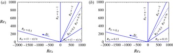
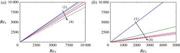
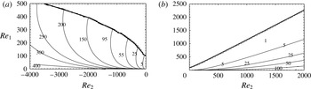
is given by (3.5). Figure 1 shows, for a thin gap (
 ${\it\eta}=0.881$
), some particular values of
 $R_{{\it\Omega}}$
in the usual parameter space (
 $\mathit{Re}_{1},\mathit{Re}_{2}$
) for a Newtonian fluid and for a power-law fluid with
 $n=0.3$
. Shear-thinning effects introduce a slight deviation of the constant
 $R_{{\it\Omega}}$
lines. For a wide gap, the deviation is much more pronounced.
Parameters of Dubrulle et al. (Reference Dubrulle, Dauchot, Daviaud, Longaretti, Richard and Zhan2005) represented in the
 $(\mathit{Re}_{1},\,\mathit{Re}_{2})$
plane at
 ${\it\eta}=0.881$
. Contours of rotation number
 $R_{{\it\Omega}}$
for (a) Newtonian fluid and (b) power-law fluid with
 $n=0.3$
. The arrow indicates that
 $\mathit{Re}$
increases along the constant
 $R_{{\it\Omega}}$
line.

For Carreau fluids,
 $\bar{r},\,Re$
and
 $R_{{\it\Omega}}$
are evaluated numerically. The constant
 $R_{{\it\Omega}}$
lines are similar to those of figure 1(b), and are therefore not represented. In the following, we have chosen to express most of our result in the
 $(\mathit{Re}_{1},\mathit{Re}_{2})$
plane, because we believe it is more understandable for the reader. In appendix D, some results for marginal stability are presented in the plane
 $(\mathit{Re},R_{{\it\Omega}})$
. As far as the transient growth is concerned, based on the work of Maretzke et al. (Reference Maretzke, Hof and Avila2014), we will use the
 $(\mathit{Re},R_{{\it\Omega}})$
representation in order to obtain a scaling of the energy growth.
3. Base flows
The base flow is azimuthal and is solution of
 $$\begin{eqnarray}\frac{\text{d}}{\text{d}r}(r^{2}{\it\tau}_{r{\it\theta}}^{b})=0,\end{eqnarray}$$
with the boundary conditions
 $$\begin{eqnarray}V^{b}(R_{1})=1\quad \text{and}\quad V^{b}(R_{2})=\frac{\mathit{Re}_{2}}{\mathit{Re}_{1}}.\end{eqnarray}$$
Hereafter, we describe the velocity and the viscosity profiles for power-law and Carreau fluids in the cases of a thin gap and a wide gap,
 ${\it\eta}=0.881$
and
 ${\it\eta}=0.4$
respectively.
3.1. Power-law fluid
The velocity profile is (Bird et al. Reference Bird, Amstrong and Hassager1987)
 $$\begin{eqnarray}V^{b}(r)=A_{0}r+\frac{B_{0}r}{r^{2/n}}\end{eqnarray}$$
with
 $$\begin{eqnarray}\displaystyle & \displaystyle A_{0}=\frac{1}{R_{1}}\left[1+\frac{1}{R_{1}^{2/n}}\left(1-\frac{\mathit{Re}_{2}}{\mathit{Re}_{1}}\,{\it\eta}\right)\left(\frac{1}{R_{2}^{2/n}}-\frac{1}{R_{1}^{2/n}}\right)^{-1}\right] & \displaystyle\end{eqnarray}$$
 $$\begin{eqnarray}\displaystyle & \displaystyle B_{0}=-\frac{1}{R_{1}}\left[\left(1-\frac{\mathit{Re}_{2}}{\mathit{Re}_{1}}\,{\it\eta}\right)\left(\frac{1}{R_{2}^{2/n}}-\frac{1}{R_{1}^{2/n}}\right)^{-1}\right]. & \displaystyle\end{eqnarray}$$
 ${\it\eta}=0.4$
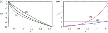
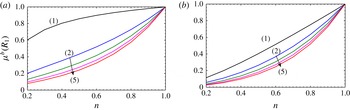
. With increasing shear-thinning effects, the curvature of the velocity profile becomes more pronounced, see figure 2(a). The shear rate increases at the inner wall and decreases at the outer wall. The wider the gap the more this effect is significant. This results in a viscosity stratification within the gap, see figure 2(b). The viscosity as well as the degree of the viscosity stratification increases from the inner wall to the outer wall. This is more pronounced with increasing shear-thinning effects (decreasing
 $n$
). Note that, for given
 $\mathit{Re}_{1}$
and
 $\mathit{Re}_{2}$
, the viscosity at the inner wall decreases with increasing shear-thinning effects, see figure 3. This variation is more pronounced for a large gap than for a thin gap.
Base flow for power-law fluids in the case of counter-rotating cylinders with
 ${\it\eta}=0.4$
,
 $\mathit{Re}_{1}=300$
and
 $\mathit{Re}_{2}=-3000$
. (a) Velocity profiles and (b) viscosity profiles for (1)
 $n=1$
(Newtonian fluid) (2)
 $n=0.5$
and (3)
 $n=0.3$
. (–
 $+$
–) Velocity profile for a Carreau fluid with
 $n=0.5$
and
 ${\it\lambda}=10$
.

Viscosity at the wall of the inner cylinder as function of the shear-thinning index
 $n$
for
 $\mathit{Re}_{1}=300$
and (1)
 $\mathit{Re}_{2}=0$
, (2)
 $\mathit{Re}_{2}=-1000$
, (3)
 $\mathit{Re}_{2}=-2000$
(4)
 $\mathit{Re}_{2}=-3000$
and (5)
 $\mathit{Re}_{2}=-4000$
: (a)
 ${\it\eta}=0.881$
, (b)
 ${\it\eta}=0.4$
.

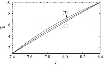
Figure 4 shows an example of a velocity profile for co-rotating cylinders. The same characteristics as for counter-rotating cylinders are observed, except that the velocity profile is convex instead of concave.
Base flow for power-law fluids in the case of co-rotating cylinders with
 ${\it\eta}=0.881$
,
 $\mathit{Re}_{1}=300$
and
 $\mathit{Re}_{2}=3000$
, (1)
 $n=1$
(Newtonian fluid), (2)
 $n=0.5$
and (3)
 $n=0.3$
.

3.2. Carreau fluid
Since no analytical expression of the velocity profile exists in this case, equation (3.1) is solved numerically using an iterative process combined with a Chebyshev polynomial approximation of the velocity profile. Details can be found in Alibenyahia et al. (Reference Alibenyahia, Lemaitre, Nouar and Ait-Messaoudene2012). For a given value of
 ${\it\lambda}$
, the effect of index
 $n$
is similar to the effect of the power-law fluid index. When increasing
 ${\it\lambda}$
, the base flow tends to that of a power-law fluid. This is observed for values of
 ${\it\lambda}$
as low as
 ${\it\lambda}=10$
(figure 2).
4. Solid rotation and Rayleigh lines
The solid rotation line corresponds to the situation where
 $\hat{{\it\Omega}}_{1}=\hat{{\it\Omega}}_{2}$
and
 $\mathit{Re}_{1}={\it\eta}\mathit{Re}_{2}$
. It is represented with dashed lines in figure 5. In the parametrization of Dubrulle et al. (Reference Dubrulle, Dauchot, Daviaud, Longaretti, Richard and Zhan2005), the solid line is given by
 $R_{{\it\Omega}}=\pm \infty$
.
Rayleigh line for a power-law fluid with (a)
 ${\it\eta}=0.881$
and (b)
 ${\it\eta}=0.4$
: (1) Newtonian fluid
 $n=1$
, (2)
 $n=0.5$
, (3)
 $n=0.2$
and (4)
 $n=0.1$
. (– – –) solid rotation line.

As indicated in the introduction, the instability of the Taylor–Couette flow is due to the stratification of the angular momentum. When the cylinders are co-rotating, the Rayleigh stable regime for an inviscid fluid is defined by
 $\text{d}/\text{d}r(L^{2})>0,\forall r\in [R_{1},R_{2}]$
, where
 $L=rV^{b}$
is the angular momentum (Drazin & Reid Reference Drazin and Reid1981). This regime is bounded in the (
 $\mathit{Re}_{1},\mathit{Re}_{2}$
) plane by the Rayleigh line, on which
 $\exists r$
such that
 $\text{d}/\text{d}r(L^{2})=0$
. For a Newtonian fluid, the Rayleigh line equation reads
 $$\begin{eqnarray}\mathit{Re}_{1}={\displaystyle \frac{\mathit{Re}_{2}}{{\it\eta}}}.\end{eqnarray}$$
Following the same approach for the non-Newtonian models considered here, the Rayleigh criterion is derived straightforwardly.
For the power-law model, we obtain
 $$\begin{eqnarray}\mathit{Re}_{1}=\left(\frac{1}{n({\it\eta}^{2/n}-1)+1}\right){\it\eta}\,\mathit{Re}_{2}.\end{eqnarray}$$
For the Carreau model, the Rayleigh line is computed numerically. As expected, for sufficiently large
 ${\it\lambda}$
, say
 ${\it\lambda}>10$
, we recover the power-law results for the same
 $n$
. Decreasing
 ${\it\lambda}$
reduces the shear-thinning effects and tends progressively to the Newtonian case.
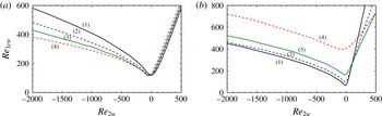
As illustrated in figure 5(a,b), with increasing shear-thinning effects (decreasing
 $n$
or increasing
 ${\it\lambda}$
) the Rayleigh line approaches the solid rotation line, thus reducing the so-called quasi-Keplerian zone, which is delimited by these two lines in the plane (
 $\mathit{Re}_{1},\mathit{Re}_{2}$
). In the quasi-Keplerian regime, the angular velocity decreases radially while the angular momentum increases radially.
Note that, for a Newtonian fluid, the Rayleigh line corresponds to
 $R_{{\it\Omega}}=-1$
. For a shear-thinning fluid, the calculations show that the Rayleigh line deviates from
 $R_{{\it\Omega}}=-1$
. This effect is more significant for a large gap and strong shear-thinning effects. For instance, for a power-law fluid with
 $n=0.3$
and
 ${\it\eta}=0.4$
, the Rayleigh line corresponds to
 $R_{{\it\Omega}}=-3.17$
.
5. Linear perturbation equations
In a classical way, we superimposed on the base flow an infinitesimal perturbation
 $$\begin{eqnarray}\{\boldsymbol{U},P,{\bf\tau}\}=\{\boldsymbol{U}^{b},P^{b},{\bf\tau}^{b}\}+{\it\epsilon}\{\boldsymbol{u}^{\prime },p^{\prime },{\bf\tau}^{\prime }\}.\end{eqnarray}$$
Substituting (
 $\boldsymbol{U},P,{\bf\tau}$
) by their expression (5.1) in (2.1) and (2.2), and linearizing around the base flow, we obtain the perturbation equations
 $$\begin{eqnarray}\displaystyle & \boldsymbol{{\rm\nabla}}\boldsymbol{\cdot }\boldsymbol{u}^{\prime }=0, & \displaystyle\end{eqnarray}$$
 $$\begin{eqnarray}\displaystyle & \displaystyle \frac{\partial \boldsymbol{u}^{\prime }}{\partial t}+\mathit{Re}_{1}[(\boldsymbol{U}^{b}\boldsymbol{\cdot }\boldsymbol{{\rm\nabla}})\boldsymbol{u}^{\prime }+(\boldsymbol{u}^{\prime }\boldsymbol{\cdot }\boldsymbol{{\rm\nabla}})\boldsymbol{U}^{\boldsymbol{b}}]=-\boldsymbol{{\rm\nabla}}p^{\prime }+\boldsymbol{{\rm\nabla}}\boldsymbol{\cdot }{\bf\tau}^{\prime }, & \displaystyle\end{eqnarray}$$
 $$\begin{eqnarray}{\bf\tau}^{\prime }=\frac{1}{{\it\epsilon}}\{{\bf\tau}(\boldsymbol{U}^{b}+{\it\epsilon}\boldsymbol{u}^{\prime })-{\bf\tau}(\boldsymbol{U}^{b})\}={\it\mu}^{b}\dot{{\bf\gamma}}(\boldsymbol{u}^{\prime })+({\it\mu}_{t}-{\it\mu}^{b})\unicode[STIX]{x1D63C}\end{eqnarray}$$
is the perturbation of the deviatoric shear-stress tensor. The components of tensor
 $\unicode[STIX]{x1D63C}$
are all zero except for
 $\unicode[STIX]{x1D608}_{1,2}=\unicode[STIX]{x1D608}_{2,1}=\dot{{\it\gamma}}_{r{\it\theta}}(\boldsymbol{u}^{\prime })$
. We have introduced in (5.4) the tangential viscosity
 ${\it\mu}_{t}$
, given by
 $$\begin{eqnarray}{\it\mu}_{t}={\it\mu}(\boldsymbol{U}^{b})+\frac{\partial {\it\mu}}{\partial \dot{{\it\gamma}}_{r{\it\theta}}}(\boldsymbol{U}^{b})\dot{{\it\gamma}}_{r{\it\theta}}(\boldsymbol{U}^{b}).\end{eqnarray}$$
We obtain the system
 $$\begin{eqnarray}\displaystyle 0 & = & \displaystyle D_{\ast }u^{\prime }+\frac{1}{r}\frac{\partial v^{\prime }}{\partial {\it\theta}}+\frac{\partial w^{\prime }}{\partial z},\end{eqnarray}$$
 $$\begin{eqnarray}\displaystyle \frac{\partial u^{\prime }}{\partial t} & = & \displaystyle -\mathit{Re}_{1}\frac{V^{b}}{r}\left(\frac{\partial u^{\prime }}{\partial {\it\theta}}-2v^{\prime }\right)-Dp^{\prime }+{\it\mu}^{b}\left[{\rm\Delta}u^{\prime }-2\frac{1}{r^{2}}\frac{\partial u^{\prime }}{\partial {\it\theta}}-\frac{u^{\prime }}{r^{2}}\right]\nonumber\\ \displaystyle & & \displaystyle +\,2D{\it\mu}^{b}Du^{\prime }+\frac{1}{r}\frac{\partial ({\it\mu}_{t}-{\it\mu}^{b})}{\partial {\it\theta}}\left(\tilde{D}v^{\prime }+\frac{1}{r}\frac{\partial u^{\prime }}{\partial {\it\theta}}\right),\end{eqnarray}$$
 $$\begin{eqnarray}\displaystyle \frac{\partial v^{\prime }}{\partial t} & = & \displaystyle -\mathit{Re}_{1}\left(u^{\prime }D_{\ast }V^{b}+\frac{V^{b}}{r}\frac{\partial v^{\prime }}{\partial {\it\theta}}\right)-\frac{1}{r}\frac{\partial p^{\prime }}{\partial {\it\theta}}+{\it\mu}^{b}\left[{\rm\Delta}v^{\prime }+\frac{2}{r^{2}}\frac{\partial u^{\prime }}{\partial {\it\theta}}-\frac{v^{\prime }}{r^{2}}\right]\nonumber\\ \displaystyle & & \displaystyle +\,D{\it\mu}^{b}\left[Dv^{\prime }-\frac{v^{\prime }}{r}+\frac{1}{r}\frac{\partial u^{\prime }}{\partial {\it\theta}}\right]+D_{\ast }\left[({\it\mu}_{t}-{\it\mu}^{b})\left(\tilde{D}v^{\prime }+\frac{1}{r}\frac{\partial u^{\prime }}{\partial {\it\theta}}\right)\right]\nonumber\\ \displaystyle & & \displaystyle +\,({\it\mu}_{t}-{\it\mu}^{b})\left[\frac{1}{r}\left(\tilde{D}v^{\prime }+\frac{1}{r}\frac{\partial u^{\prime }}{\partial {\it\theta}}\right)\right],\end{eqnarray}$$
 $$\begin{eqnarray}\displaystyle \frac{\partial w^{\prime }}{\partial t} & = & \displaystyle -\mathit{Re}_{1}\frac{V^{b}}{r}\frac{\partial w^{\prime }}{\partial {\it\theta}}-\frac{\partial p^{\prime }}{\partial z}+{\it\mu}^{b}{\rm\Delta}w^{\prime }+D{\it\mu}^{b}\left[Dw^{\prime }+\frac{\partial u^{\prime }}{\partial z}\right],\end{eqnarray}$$
 $D=\partial /\partial r,\,D_{\ast }=D+(1/r)$
,
 $\tilde{D}=D-(1/r)$
and
 ${\it\Delta}=D^{2}+(1/r)D+((1/r)(\partial /\partial {\it\theta}))^{2}+(\partial /\partial z)^{2}$
.
The boundary conditions are obtained by assuming no slip and impermeability at inner and outer walls,
 $$\begin{eqnarray}\boldsymbol{u}^{\prime }=0\quad \text{at }r=R_{1},\,R_{2}.\end{eqnarray}$$
The linear system (5.6)–(5.9) is homogeneous in the axial and azimuthal directions. Perturbations can thus be decomposed into Fourier modes with an azimuthal wavenumber
 $m\in \mathbb{Z}$
and an axial wavenumber
 $k\in \mathbb{R}$
:
 $$\begin{eqnarray}\{\boldsymbol{u}^{\prime },p^{\prime }\}=\{\tilde{\boldsymbol{u}}(r,t),\tilde{p}(r,t)\}\exp [\text{i}(m{\it\theta}+kz)]+\text{c.c.},\end{eqnarray}$$
where c.c. stands for the complex conjugate and
 $\tilde{\boldsymbol{u}}(r,t)=\tilde{u} (r,t)\,\boldsymbol{e}_{r}+\tilde{v}(r,t)\,\boldsymbol{e}_{{\it\theta}}+\tilde{w}(r,t)\,\boldsymbol{e}_{z}$
. By eliminating the pressure and one velocity component, the resulting system can be written in terms of two components of the velocity
 $(\tilde{u} ,\tilde{v})$
for
 $k\neq 0$
or
 $(\tilde{u} ,\tilde{w})$
for
 $m\neq 0$
. The different formulations lead to an initial value problem which can be written formally as
 $$\begin{eqnarray}\mathscr{L}\tilde{\boldsymbol{q}}=\mathscr{M}\,\frac{\partial \tilde{\boldsymbol{q}}}{\partial t}\end{eqnarray}$$
where
 $\tilde{\boldsymbol{q}}=(\tilde{u} ,\tilde{v})^{\text{T}}$
or
 $(\tilde{u} ,\tilde{w})^{\text{T}}$
, depending on the formulation adopted. The linear operators
 $\mathscr{L}$
and
 $\mathscr{M}$
are given in appendix A.
6. Long-time behaviour of the disturbance: eigenvalue problem
The initial value problem can be turned into an eigenvalue problem by the assumption of the exponential time dependence, i.e.
 $\tilde{\boldsymbol{q}}(r,t)=\boldsymbol{q}(r)\exp ({\it\sigma}t)$
. The resulting generalized eigenvalue problem reads
 $$\begin{eqnarray}\mathscr{L}\boldsymbol{q}={\it\sigma}\mathscr{M}\boldsymbol{q}\end{eqnarray}$$
with the complex frequency
 ${\it\sigma}$
as the eigenvalue. The real part of
 ${\it\sigma}$
is the growth rate of the perturbation and its imaginary part is its oscillation frequency. The eigenvalue problem (6.1) is discretized using a spectral collocation method based on Chebyshev polynomials evaluated at
 $N$
collocation points of the Gauss–Lobatto method. The matrix eigenvalue problem that results is solved using the QZ algorithm with Matlab. To ensure the convergence of the numerical method, computations were performed for increasing
 $N$
. It was found that, for
 $N\geqslant 40$
, the five first eigenvalues remain unchanged with three digits accuracy. Each computation was then performed for
 $N$
and
 $N+5$
, and only the overlapping eigenvalues were retained. This procedure allows one to remove spurious eigenvalues.
6.1. Eigenvalue spectra
In this section, eigenspectra are analysed for axisymmetric and non-axisymmetric perturbations. For both situations, the inner Reynolds number
 $\mathit{Re}_{1}$
is fixed and the outer Reynolds number
 $\mathit{Re}_{2}$
is varied. Then,
 $\mathit{Re}_{2}$
is fixed and
 $\mathit{Re}_{1}$
is increased until marginal stability is reached.
6.1.1. Axisymmetric perturbation
$m=0$

The perturbation is 2D and the
 $(\tilde{u} ,\tilde{v})$
formulation is used. As
 $m=0$
, the linear operators
 $\mathscr{L}$
and
 $\mathscr{M}$
, given by equations (A 2)–(A 7) in appendix A, are real. Therefore, the eigenvalues are real or complex conjugate. Spectra for that case are presented in figure 6 for a Newtonian fluid.
Eigenspectra for a Newtonian fluid undergoing an axisymmetric perturbation
 $m=0$
for
 ${\it\eta}=0.881$
,
 $k={\rm\pi}$
,
 $\mathit{Re}_{1}=400$
, and varying
 $\mathit{Re}_{2}$
. (a)
 $\mathit{Re}_{2}=352.4$
(on the Rayleigh line) and (b) (●)
 $\mathit{Re}_{2}=-4000$
, (○)
 $\mathit{Re}_{2}=-25\,000$
.

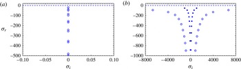
On the Rayleigh line, the angular momentum is constant. The spectrum, figure 6(a), consists of a vertical branch with real eigenvalues. It is independent of
 $\mathit{Re}_{1}$
, as indicated by Gebhardt & Grossmann (Reference Gebhardt and Grossmann1993). These properties are demonstrated in appendix B.
When the outer cylinder is fixed,
 $\mathit{Re}_{2}=0$
, most of the eigenvalues are real. DiPrima & Hall (Reference DiPrima and Hall1984) have shown that the first eigenvalue that crosses the real axis is always real, in agreement with the principle of stability exchange.
For counter-rotating cylinders, the real vertical branch, which is made of paired eigenvalues, splits into two lateral curved branches, i.e. one pair of eigenvalues separates into two complex conjugate eigenvalues, see figure 6(b). The higher the absolute value of
 $\mathit{Re}_{2}$
, the lower the locus of the branch separation. The imaginary parts of the spectra are bounded by the epicyclic frequency
 ${\it\kappa}$
evaluated at the outer wall,
 $r=R_{2}$
(Shu Reference Shu1982). The epicyclic frequency is defined by
 $$\begin{eqnarray}{\it\kappa}^{2}(r)=\left(-\frac{1}{r^{3}}\frac{\text{d}}{\text{d}r}(rV)^{2}\right).\end{eqnarray}$$
For a Newtonian fluid at
 $r=R_{2}$
,
 $$\begin{eqnarray}{\it\kappa}^{2}(R_{2})=4\mathit{Re}_{2}(\mathit{Re}_{2}-{\it\eta}\mathit{Re}_{1})\left(\frac{1-{\it\eta}}{1+{\it\eta}}\right).\end{eqnarray}$$
Similar results are observed for a wide gap.
Additional computations not presented here were conducted for co-rotating cylinders, and spectrum evolutions similar to the counter-rotating situation have been obtained.
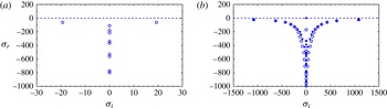
For shear-thinning fluids, the eigenspectra are quite similar to the Newtonian case. However, two differences have been noted:
-
(i) on the Rayleigh line, the angular momentum is no longer constant in the annular space, thus the eigenvalues are not necessarily real, figure 7(a). Furthermore, they vary with
$\mathit{Re}_{1}$
. -
(ii) for the same values of
$\mathit{Re}_{1}$
and
$\mathit{Re}_{2}$
, the vertical branch separation occurs closer to the real axis than for a Newtonian fluid.


Eigenspectra for a power-law fluid undergoing an axisymmetric perturbation
 $m=0$
with
 $k={\rm\pi}$
,
 $n=0.5$
,
 ${\it\eta}=0.881$
, varying
 $\mathit{Re}_{1}$
and
 $\mathit{Re}_{2}$
(a) on the Rayleigh line
 $\mathit{Re}_{2}=454.71$
,
 $\mathit{Re}_{1}=500$
(b)
 $\mathit{Re}_{2}=-4000$
, (○)
 $\mathit{Re}_{1}=500$
, (●)
 $\mathit{Re}_{1}=\mathit{Re}_{1c}=828.14$
.

The evolution of the eigenspectra, when
 $\mathit{Re}_{2}$
is fixed and
 $\mathit{Re}_{1}$
is increased until the critical value, is shown in figure 7(b) for a power-law fluid with
 $n=0.5$
. The critical mode is stationary and consists of two counter-rotating vortices. Similar results are obtained for a Carreau fluid.
6.1.2. Non-axisymmetric perturbation
$m\neq 0$

Numerical computations show no fundamental differences in the eigenspectra shape for Newtonian and shear-thinning fluids. In order not to overload the paper, we have chosen to present only the power-law results. The Carreau model provides similar results when
 ${\it\lambda}\dot{{\it\gamma}}_{r{\it\theta}}^{b}\gg 1$
, as indicated in § 2.2. The classification of the eigenspectra is less evident than in the axisymmetric case. According to Gebhardt & Grossmann (Reference Gebhardt and Grossmann1993), the structure of the eigenspectra depends on the value of the axial wavenumber relative to the modified azimuthal wavenumber
 $m/r_{m}$
with
 $r_{m}=(R_{1}+R_{2})/2$
. If
 $k\geqslant m/r_{m}$
, the spectrum structure is close to that of an azimuthal invariant flow. In contrast, if
 $k\leqslant m/r_{m}$
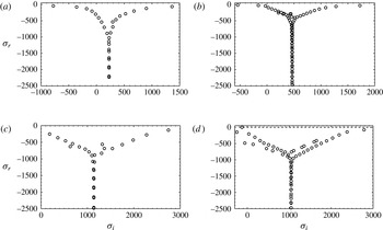
, features of an axial invariant flow dominate. Figure 8 shows that, with increasing
 $m$
, the eigenvalue spectrum evolves from a ‘jet-like’ structure (figure 8
a) characteristic of axisymmetric perturbation flow to a ‘Y-shaped’ spectrum characteristic of axial invariant perturbation (Gebhardt & Grossmann Reference Gebhardt and Grossmann1993). Figure 8(d) shows that when
 $\mathit{Re}_{1}$
is increased until marginal stability (
 ${\it\sigma}_{r}=0$
), the critical mode corresponds to time-dependent spiral vortices, with an angular phase velocity
 ${\it\omega}=-{\it\sigma}_{i}/m$
.
Eigenspectra for a power-law fluid undergoing a non-axisymmetric perturbation with
 $n=0.5,\,{\it\eta}=0.881$
. The outer Reynolds number and the axial wavenumber are fixed:
 $\mathit{Re}_{2}=-4000$
and
 $k={\rm\pi}$
respectively. (a)
 $m=1,\,\mathit{Re}_{1}=400$
, (b)
 $m=2,\,\mathit{Re}_{1}=400$
, (c)
 $m=5,\,\mathit{Re}_{1}=400$
and (d)
 $m=5$
,
 $\mathit{Re}_{1}=\mathit{Re}_{1c}=878.55$
.

6.2. Marginal stability curves
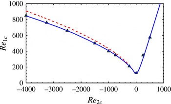
First, a validation test was performed by comparing our results against studies previously published in the literature. In figure 9 our results are compared against those obtained by Meseguer (Reference Meseguer2002) for 3D perturbations in a Newtonian fluid. A very good agreement is observed. In the case of counter-rotating cylinders, the critical
 $\mathit{Re}_{1c}$
is lower for non-axisymmetric modes (
 $m\neq 0$
) than for axisymmetric modes (
 $m=0$
), in agreement with the literature (Krueger et al.
Reference Krueger, Gross and Diprima1966; Langford et al.
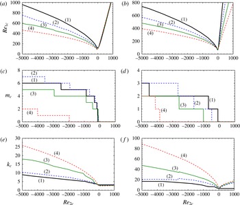
Reference Langford, Tagg, Kostelich, Swinney and Glubitsky1988). For power-law fluids, figure 10 shows the influence of the shear-thinning index on the critical conditions. Globally, for fixed
 $\mathit{Re}_{2}$
, shear thinning reduces
 $\mathit{Re}_{1c}$
, except in the neighbourhood of
 $\mathit{Re}_{2}=0$
with a large gap and for co-rotating cylinders with small gaps, where
 $\mathit{Re}_{1c}$
increases slightly. Similar evolutions are observed for Carreau fluids. For
 ${\it\lambda}\geqslant 10$
, we recover the power-law results. The decrease of
 $\mathit{Re}_{1c}$
with increasing shear-thinning effects can be analysed using the energy equation obtained by multiplying the linearized momentum equations with the complex conjugate
 $\boldsymbol{u}^{\ast }$
and integrating between the two cylinders
 $$\begin{eqnarray}\displaystyle & \displaystyle \mathscr{R}e({\it\sigma})\Vert \boldsymbol{u}\Vert ^{2}=-\mathit{Re}_{1}\,\int _{R_{1}}^{R_{2}}f(r)r\,\text{d}r-\int _{R_{1}}^{R_{2}}g_{1}(r)r\,\text{d}r+\int _{R_{1}}^{R_{2}}g_{2}(r)r\,\text{d}r\quad \text{with} & \displaystyle\end{eqnarray}$$
 $$\begin{eqnarray}\displaystyle & \displaystyle f(r)=\dot{{\it\gamma}}_{r{\it\theta}}^{b}\,\frac{u^{\ast }v+uv^{\ast }}{2} & \displaystyle\end{eqnarray}$$
 $$\begin{eqnarray}\displaystyle & g_{1}(r)={\it\mu}^{b}\left[{\textstyle \frac{1}{2}}(|\dot{{\it\gamma}}_{rr}|^{2}+|\dot{{\it\gamma}}_{{\it\theta}{\it\theta}}|^{2}+|\dot{{\it\gamma}}_{zz}|^{2})+|\dot{{\it\gamma}}_{r{\it\theta}}|^{2}+|\dot{{\it\gamma}}_{rz}|^{2}+|\dot{{\it\gamma}}_{{\it\theta}z}|^{2}\right] & \displaystyle\end{eqnarray}$$
 $$\begin{eqnarray}\displaystyle & g_{2}(r)=({\it\mu}^{b}-{\it\mu}_{t})\,|{\dot{{\it\gamma}}^{\prime }}_{r{\it\theta}}|^{2} & \displaystyle\end{eqnarray}$$
 $\Vert \boldsymbol{u}\Vert ^{2}=\int _{R_{1}}^{R_{2}}(1/2)(uu^{\ast }+vv^{\ast }+ww^{\ast })r\,\text{d}r$
.
Marginal stability curves in the plane (
 $\mathit{Re}_{1},\mathit{Re}_{2}$
) for a Newtonian fluid with
 ${\it\eta}=0.881$
: comparison with Meseguer (Reference Meseguer2002). (Continuous line) our results for 3D perturbations, (dashed line) our results for axisymmetric perturbations
 $m=0$
, (▵) Meseguer (Reference Meseguer2002).

Critical conditions of instability for a power-law fluid with two radius ratios,
 ${\it\eta}=0.881$
(figures on the left) and
 ${\it\eta}=0.4$
(figures on the right). Effect of the shear-thinning index. (a, b) Marginal stability curves in plane (
 $\mathit{Re}_{1},\mathit{Re}_{2}$
), (c, d) critical azimuthal wavenumbers, (e, f) critical axial wavenumbers. (1) Newtonian fluid,
 $n=1$
, (2)
 $n=0.7$
, (3)
 $n=0.5$
and (4)
 $n=0.3$
.

In (6.4), the first term on the right-hand side is a production term. It is associated with the work of the Reynolds stress,
 $-uv$
, on the wall-normal basic shear
 $\dot{{\it\gamma}}_{r{\it\theta}}^{b}$
. The second term represents viscous dissipation. The third term arises from the viscosity perturbation due to shear thinning; it is positive, and can thus be regarded as a source of energy for the perturbation. Following Ranganathan & Govindarajan (Reference Ranganathan and Govindarajan2001), it is convenient to compute and compare the space-averaged production and dissipation terms
 ${\it\bf\Gamma}^{+}$
and
 ${\it\bf\Gamma}^{-}$
respectively defined by
 $$\begin{eqnarray}{\it\bf\Gamma}^{+}={\displaystyle \frac{\displaystyle \mathit{Re}_{1}\,\int _{R_{1}}^{R_{2}}f(r)r\,\text{d}r}{\Vert \boldsymbol{u}\Vert ^{2}}}\quad \text{and}\quad {\it\bf\Gamma}^{-}={\displaystyle \frac{\displaystyle \int _{R_{1}}^{R_{2}}g_{1}(r)r\,\text{d}r-\int _{R_{1}}^{R_{2}}g_{2}(r)r\,\text{d}r}{\Vert \boldsymbol{u}\Vert ^{2}}}.\end{eqnarray}$$
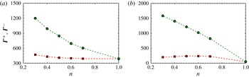
At criticality, the production term is exactly balanced by the dissipation term,
 ${\it\bf\Gamma}^{+}={\it\bf\Gamma}^{-}$
, as shown in figure 11 in the case of a Newtonian fluid. The influence of shear-thinning effects on the energy budget can be appreciated by comparing the results obtained for a Newtonian fluid with those of a power-law at the same value of
 $\mathit{Re}_{1}$
, i.e.
 $\mathit{Re}_{1}=\mathit{Re}_{1c}$
(Newtonian). The critical azimuthal and axial wavenumbers are evaluated for the parameters
 $\mathit{Re}_{1}=\mathit{Re}_{1c}$
(Newtonian),
 $\mathit{Re}_{2}$
and
 $n$
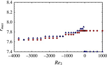
. With increasing shear-thinning effects, the average viscous dissipation remains close to that of a Newtonian fluid, while the production term increases significantly, rendering the flow less stable than in the Newtonian case. The main factor determining stability or instability of the flow is thus the exchange of energy between the base flow and the perturbation. In figure 12, the location of the maxima
 $f$
and
 $(g_{1}+g_{2})$
functions defined in (6.5)–(6.7) are plotted against
 $\mathit{Re}_{2}$
. It appears that the maxima of the energy exchange and of viscous dissipation occur near the inner cylinder. The increase of
 ${\it\bf\Gamma}^{+}$
with increasing shear-thinning effects may be attributed to the increase of the inner velocity gradient. Concerning the critical azimuthal and axial wavenumbers, in the co-rotating regime, the critical mode is axisymmetric (figure 10
c,d). The primary bifurcation leads to time-independent Taylor-vortex flow. In the case of the counter-rotating regime, the critical azimuthal wavenumber increases with
 $|\mathit{Re}_{2}|$
. There is a limit value of
 $\mathit{Re}_{2}$
, say
 $\mathit{Re}_{2s}$
, under which the primary bifurcation leads to axisymmetric toroidal structures (
 $m_{c}=0$
) and over which the bifurcation leads to spiral vortices (
 $m_{c}\geqslant 1$
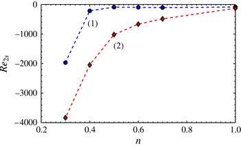
). Spiral vortices are travelling waves in axial and azimuthal directions. Figure 13 shows the variation of
 $\mathit{Re}_{2s}$
with the shear-thinning index for both a wide gap and a thin gap. For strong shear-thinning effects, the critical mode remains axisymmetric for large negative
 $\mathit{Re}_{2}$
. The axial wavelength decreases with increasingly negative
 $\mathit{Re}_{2}$
and increasing shear-thinning effects. This may be attributed to the decrease of the ‘effective gap’ where the Rayleigh instability criterion holds, i.e. the gap between the inner cylinder and the ‘nodal surface’ where
 $V^{b}=0$
.
Space average of (○) the production term
 ${\it\bf\Gamma}^{+}$
and (▫) the viscous dissipation term
 ${\it\bf\Gamma}^{-}$
defined by (6.8) for a power-law fluid with
 ${\it\eta}=0.4$
as a function of shear-thinning index,
 $n$
. (a)
 $\mathit{Re}_{2}=-2025$
, (b)
 $\mathit{Re}_{2}=500$
.


Power-law fluids. Influence of the shear-thinning index on the critical outer Reynolds number
 $\mathit{Re}_{2s}$
at which the transition to spirals takes place for (1)
 ${\it\eta}=0.881$
and (2)
 ${\it\eta}=0.4$
.

7. Short-time behaviour: transient growth and optimal perturbation
The traditional approach of stability based on eigenvalues is not sufficient to describe the temporal behaviour of the disturbance at all times because of the non-normality of the linear stability operator. This mathematical property means that there is a potential for energy extraction from the base flow by a subspace of perturbations leading to transient growth, despite the absence of exponential instability.
7.1. Transient growth and characteristics of optimal perturbation
The transient evolution of a perturbation kinetic energy in the linear regime is determined by following the methodology described by Schmid & Henningson (Reference Schmid and Henningson2001). It is presented here only for the
 $(\tilde{u} ,\tilde{v})$
formulation, but a similar development applies to the
 $(\tilde{u} ,\tilde{w})$
formulation. For a given Fourier mode, the disturbance instantaneous kinetic energy is given by
 $$\begin{eqnarray}\displaystyle \Vert \boldsymbol{q}(t)\Vert _{E}^{2} & = & \displaystyle \int _{R_{1}}^{R_{2}}\left[|\tilde{u} |^{2}+\frac{1}{k^{2}}\frac{1}{r^{2}}\left|\frac{\text{d}}{\text{d}r}(r\tilde{u} )\right|^{2}+\left(\frac{m^{2}}{r^{2}k^{2}}+1\right)|\tilde{v}|^{2}\right.\nonumber\\ \displaystyle & & \displaystyle +\,\left.\frac{\text{i}m}{kr}\left(\frac{\tilde{v}}{r}\frac{\text{d}}{\text{d}r}(r\tilde{u} ^{\ast })-\frac{\tilde{v}^{\ast }}{r}\frac{\text{d}}{\text{d}r}(r\tilde{u} )\right)\vphantom{\left|\frac{\text{d}}{\text{d}r}(r\tilde{u} )\right|^{2}}\right]\,r\,\text{d}r,\end{eqnarray}$$
which is a function of time and of the initial condition,
 $\boldsymbol{q}_{0}=(\tilde{u} _{0},\tilde{v}_{0})^{\text{T}}=\boldsymbol{q}(r,t=0,m,k)$
. The maximum kinetic energy amplification at time
 $t$
over all initial conditions is defined by
 $$\begin{eqnarray}G(t,m,k)=\sup _{\boldsymbol{q}_{0}\neq 0}\frac{\Vert \boldsymbol{q}(t)\Vert _{E}^{2}}{\Vert \boldsymbol{q}(0)\Vert _{E}^{2}}.\end{eqnarray}$$
The maximum energy transient growth over all times is
 $$\begin{eqnarray}G^{max}(m,k)=\sup _{t\geqslant 0}G(t,m,k).\end{eqnarray}$$
The maximum of
 $G^{max}$
over all pairs
 $(m,k)$
, denoted
 $G^{opt}$
, is reached by the optimal perturbation at time
 $t^{opt}$
.
First, we performed validation tests for a Newtonian fluid. In table 1, our results are compared against those of Meseguer (Reference Meseguer2002) and Maretzke et al. (Reference Maretzke, Hof and Avila2014). Very good agreement is observed. The conditions of Hristova et al. (Reference Hristova, Roch, Schmid and Tuckerman2002) given in their table II were also simulated. A relative discrepancy of less than 1 % was obtained.
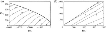
Contours of optimal energy growth
 $G^{opt}$
in the plane (
 $\mathit{Re}_{1},\mathit{Re}_{2}$
) for a Newtonian fluid with
 ${\it\eta}=0.881$
: (a) counter-rotating cylinders, (b) co-rotating cylinders. The thick line is the marginal stability curve.

Comparison of the present results with those of Meseguer (Reference Meseguer2002) and Maretzke et al. (Reference Maretzke, Hof and Avila2014) at the same Reynolds numbers and
 ${\it\eta}=0.881$
.

As a reference case, we further studied the transient growth for a Newtonian fluid. Figure 14 shows contours of the optimal growth for a Newtonian fluid in the plane
 $(\mathit{Re}_{1},\mathit{Re}_{2})$
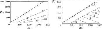
. The corresponding axial and azimuthal wavenumbers are represented in figures 15 and 16. It is interesting to observe that, in the counter-rotating regime, the optimal azimuthal wavenumber varies little (
 $10<m^{opt}<13$
) and is much higher than the critical wavenumber
 $m_{c}$
. Concerning
 $k^{opt}$
, it is smaller than the critical axial wavenumber
 $k_{c}$
.
Contours of optimal wavenumbers in the (
 $\mathit{Re}_{1},\mathit{Re}_{2}$
) plane for a Newtonian fluid flowing between counter-rotating cylinders with
 ${\it\eta}=0.881$
. (a) Optimal azimuthal wavenumber
 $m^{opt}$
and (b) optimal axial wavenumber
 $k^{opt}$
. The thick line is the marginal stability curve.

Contours of optimal wavenumbers in the (
 $\mathit{Re}_{1},\mathit{Re}_{2}$
) plane for a Newtonian fluid flowing between co-rotating cylinders with
 ${\it\eta}=0.881$
. (a) Optimal azimuthal wavenumber
 $m^{opt}$
and (b) optimal axial wavenumber
 $k^{opt}$
. The thick line is the marginal stability curve.

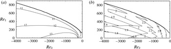
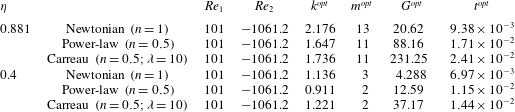
For a shear-thinning fluid, the contours of optimal energy amplification are shown in figure 17. The amplification appears to be much larger than for a Newtonian fluid. In table 2, the optimal growth conditions
 $G^{opt}$
,
 $k^{opt}$
,
 $m^{opt}$
and
 $t^{opt}$
are compared for Newtonian, power-law and Carreau fluids at given
 $\mathit{Re}_{1}$
and
 $\mathit{Re}_{2}$
for thin and wide gaps. It is observed that the optimal amplification is highest for a Carreau fluid and at a thin gap. The optimal azimuthal and axial wavenumbers are practically the same for Newtonian and shear-thinning fluids. The optimal time is greater for power-law fluids, and even greater for Carreau fluids.
Contours of optimal energy growth
 $G^{opt}$
in the plane (
 $\mathit{Re}_{1},\mathit{Re}_{2}$
) for a power-law fluid with
 $n=0.5$
and
 ${\it\eta}=0.881$
: (a) counter-rotating cylinders, (b) co-rotating cylinders. The thick line is the marginal stability curve.

These results may be presented in a concise manner by using the shear Reynolds number
 $\mathit{Re}$
and the rotation number
 $R_{{\it\Omega}}$
. This representation is more relevant in the determination of scaling laws for the optimal energy amplification (Maretzke et al.
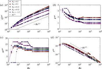
Reference Maretzke, Hof and Avila2014). Figure 18 shows the characteristics of the optimal perturbation as a function of
 $\mathit{Re}$
for different values of
 $R_{{\it\Omega}}$
. We recover the scaling
 $G^{opt}\propto \mathit{Re}^{2/3}$
for sufficiently large
 $\mathit{Re}$
, as indicated by Maretzke et al. (Reference Maretzke, Hof and Avila2014). The optimal azimuthal wavenumber varies slightly with
 $R_{{\it\Omega}}$
. At
 ${\it\eta}=0.881$
, figure 18(c) shows again that asymptotically
 $10\leqslant m^{opt}\leqslant 13$
. In this range of
 $m^{opt}$
, the kinetic energy amplification does not change significantly. Concerning the axial wavenumber, it is observed that it is much lower than the linear critical wavenumber
 $k_{c}$
, see figure 18(b). The optimal time
 $t^{opt}$
decreases asymptotically as
 $t^{opt}\propto \mathit{Re}^{-2/3}$
.
Optimal energy growth and characteristics of the optimal perturbation as a function of the shear Reynolds number
 $\mathit{Re}$
for different values of the rotation number
 $R_{{\it\Omega}}$
. Newtonian fluid with
 ${\it\eta}=0.881$
. (a) Optimal energy growth
 $G^{opt}$
, (b) optimal axial wavenumber
 $k^{opt}$
, (c) optimal azimuthal wavenumber
 $m^{opt}$
and (d) optimal time
 $t^{opt}$
.

Comparison of the optimal energy growth at
 ${\it\eta}=0.881$
and
 ${\it\eta}=0.4$
for the different fluid models considered.

For the particular case of
 $R_{{\it\Omega}}=-1$
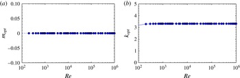
, i.e. along the Rayleigh line, the optimal perturbation is axisymmetric with
 $k^{opt}\approx {\rm\pi}$
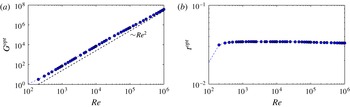
, as shown by figure 19. The optimal amplification varies as
 $G^{opt}\propto \mathit{Re}^{2}$
(figure 20). The optimal time at which
 $G^{opt}$
is reached decreases very slightly with
 $\mathit{Re}$
.
Structure of the optimal perturbation along the Rayleigh line (
 $R_{{\it\Omega}}=-1$
) for a Newtonian fluid and
 ${\it\eta}=0.881$
. (a) Azimuthal and (b) axial wavenumbers as a function of the shear Reynolds number.

(a) Optimal energy growth and (b) optimal time versus shear Reynolds number along the Rayleigh line (
 $R_{{\it\Omega}}=-1$
) for a Newtonian fluid with
 ${\it\eta}=0.881$
.

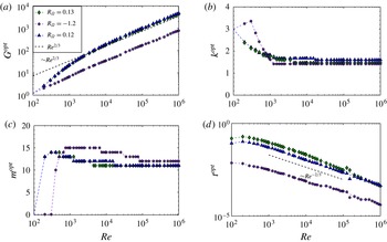
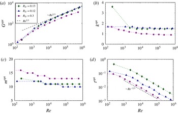
The characteristics of optimal perturbations were also determined for power-law and Carreau fluids. They are represented in figures 21 and 22, respectively. It is interesting to note that we recover the same scaling as for a Newtonian fluid. Indeed, at large
 $\mathit{Re}$
,
 $G^{opt}\propto \mathit{Re}^{2/3}$
;
 $t^{opt}\propto \mathit{Re}^{-2/3}$
;
 $10\leqslant m^{opt}\leqslant 13$
and
 $1\leqslant k^{opt}<2$
much lower than
 $k_{c}$
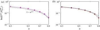
. Comparison with the Newtonian case indicates that, for given
 $\mathit{Re}$
and
 $R_{{\it\Omega}}$
,
 $G^{opt}$
increases with increasing shear-thinning degree, as shown in figure 23. This is related to the increase of the non-normality of the linear operator. The approximate scaling is found:
 $$\begin{eqnarray}\frac{G^{opt}}{G_{n=1}^{opt}}\propto {\it\kappa}\exp (-n^{{\it\alpha}})\end{eqnarray}$$
where
 ${\it\kappa}$
is a constant,
 $G_{n=1}^{opt}$
is the optimal energy growth for a Newtonian fluid and
 ${\it\alpha}=1/3$
.
Optimal energy growth and characteristics of the optimal perturbation as a function of the shear Reynolds number
 $\mathit{Re}$
for different values of the rotation number
 $R_{{\it\Omega}}$
. Power-law fluid with
 $n=0.5$
and
 ${\it\eta}=0.881$
. (a) Optimal energy growth
 $G^{opt}$
, (b) optimal axial wavenumber
 $k^{opt}$
, (c) optimal azimuthal wavenumber
 $m^{opt}$
and (d) optimal time
 $t^{opt}$
.

Optimal energy growth and characteristics of the optimal perturbation as a function of the shear Reynolds number for different values of the rotation number
 $R_{{\it\Omega}}$
. Carreau fluid with
 $n=0.5$
,
 ${\it\lambda}=10$
and
 ${\it\eta}=0.881$
. (a) Optimal energy growth
 $G^{opt}$
, (b) optimal axial wavenumber
 $k^{opt}$
, (c) optimal azimuthal wavenumber
 $m^{opt}$
and (d) optimal time
 $t^{opt}$
.

Shear-thinning effect on the optimal energy growth for a power-law fluid with
 ${\it\eta}=0.881$
, at different shear Reynolds numbers and fixed
 $R_{{\it\Omega}}$
. (a)
 $R_{{\it\Omega}}=0.12$
,
 $10^{4}\leqslant Re\leqslant 10^{5}$
and (b)
 $R_{{\it\Omega}}=0.1$
,
 $5\times 10^{3}\leqslant Re\leqslant 10^{4}$
.

7.2. Evolution of the optimal perturbation: transient growth mechanism
In this section, the optimal perturbation and its time evolution are described for different values of
 $\mathit{Re}_{1}$
and
 $\mathit{Re}_{2}$
in the linearly stable domain.
7.2.1. Newtonian fluids
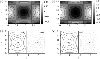
For Newtonian fluids, numerical results show that the Rayleigh line should be distinguished from the rest of the domain. The contours of the azimuthal vorticity and azimuthal velocity of the optimal perturbation at initial time
 $t=0$
and optimal time
 $t=t^{opt}$
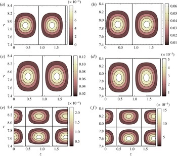
are presented in figure 24. It appears that the optimal perturbation is a superposition along the axial direction of high and low azimuthal velocity streaks. Figure 25 shows the contours of the local kinetic energy associated with the azimuthal, radial and axial components of the velocity perturbation. At initial time, more than 99 % of the kinetic energy of the perturbation is concentrated in the azimuthal component. At optimal time,
 $t=t^{opt}$
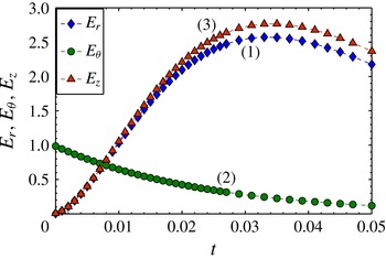
, the kinetic energy is merely concentrated in the radial and axial components. This is also illustrated in figure 26, where we have represented the spatial average of the kinetic energy contained in a volume
 $\mathscr{V}=2{\rm\pi}^{2}(R_{2}^{2}-R_{1}^{2})/k$
,
 $$\begin{eqnarray}E_{r}=\frac{1}{\mathscr{V}}\langle \tilde{u} \tilde{u} ^{\ast }\rangle ;\quad E_{{\it\theta}}=\frac{1}{\mathscr{V}}\langle \tilde{v}\tilde{v}^{\ast }\rangle ;\quad E_{z}=\frac{1}{\mathscr{V}}\langle \tilde{w}\tilde{w}^{\ast }\rangle\end{eqnarray}$$
with
 $$\begin{eqnarray}\langle .\rangle =\int _{R_{1}}^{R_{2}}\int _{0}^{2{\rm\pi}}\int _{0}^{2{\rm\pi}/k}(.)r\,\text{d}r\,\text{d}{\it\theta}\,\text{d}z.\end{eqnarray}$$
Optimal perturbation represented in the plane (
 $r,z$
) for a Newtonian fluid along the Rayleigh line,
 ${\it\eta}=0.881$
,
 $\mathit{Re}_{1}=1135$
and
 $\mathit{Re}_{2}=1000$
, with
 $m^{opt}=0$
,
 $k^{opt}=3.32$
and
 $G^{opt}=5.58$
. Contours of the azimuthal vorticity component at (a)
 $t=0$
and (b) optimal time
 $t=t^{opt}$
. Contours of the azimuthal velocity component at (c)
 $t=0$
,
 $v_{max}=0.52$
and (d) optimal time
 $t=t^{opt}$
,
 $v_{max}=0.1$
; the contours are normalized by the maximum velocity at time
 $t$
and shown in steps of 0.2. The solid lines represent positive values and the dotted lines represent negative values.

Optimal perturbation represented in plane (
 $r,z$
) for a Newtonian fluid along the Rayleigh line with
 ${\it\eta}=0.881$
,
 $\mathit{Re}_{1}=1135$
,
 $\mathit{Re}_{2}=1000$
,
 $m^{opt}=0$
,
 $k^{opt}=3.32$
and
 $G^{opt}=5.58$
. Contours of the radial component of the kinetic energy
 $1/2~u^{\prime 2}(t)$
at (a) initial time
 $t=0$
and (b) optimal time
 $t=t^{opt}$
. Contours of the azimuthal component of the kinetic energy
 $1/2~v^{\prime 2}(t)$
at (c) initial time
 $t=0$
and (d) optimal time
 $t=t^{opt}$
. Contours of the axial component of the kinetic energy
 $1/2~w^{\prime 2}(t)$
at (e)
 $t=0$
and (f) optimal time
 $t=t^{opt}$
.

Radial (1), azimuthal (2) and axial (3) kinetic energy components on the Rayleigh line for a Newtonian fluid with
 ${\it\eta}=0.881$
,
 $m^{opt}=0$
,
 $k^{opt}=3.32$
,
 $G^{opt}=5.58$
,
 $\mathit{Re}_{1}=1135$
and
 $\mathit{Re}_{2}=1000$
.

The optimal perturbation, which is initially in the form of azimuthal streaks, transforms progressively through the anti-lift-up mechanism (Antkowiak & Brancher Reference Antkowiak and Brancher2007) into azimuthal rolls. This scenario observed in rotating flows is opposite to the classical lift-up mechanism, active for instance in plane shear flows, where weak streamwise rolls give rise to strong streamwise streaks. Antkowiak & Brancher (Reference Antkowiak and Brancher2007), proposed two ways of explaining the anti-lift-up scenario.
First, it can be illustrated by considering the linearized perturbation equations for the azimuthal velocity
 $v^{\prime }$
and the azimuthal vorticity
 ${\it\omega}_{{\it\theta}}^{\prime }=\partial u^{\prime }/\partial z-\partial w^{\prime }/\partial r$
for an axisymmetric perturbation:
 $$\begin{eqnarray}\displaystyle & \displaystyle \frac{\partial v^{\prime }}{\partial t}={\rm\Delta}v^{\prime }, & \displaystyle\end{eqnarray}$$
 $$\begin{eqnarray}\displaystyle & \displaystyle \frac{\partial {\it\omega}_{{\it\theta}}^{\prime }}{\partial t}=-2\,\mathit{Re}_{1}{\it\Omega}^{b}\frac{\partial v^{\prime }}{\partial z}+{\rm\Delta}{\it\omega}_{{\it\theta}}^{\prime }, & \displaystyle\end{eqnarray}$$
 ${\it\Omega}^{b}=V^{b}/r$
is the basic angular velocity. The azimuthal velocity satisfies a diffusion equation, and decreases viscously. Whereas the azimuthal vorticity is driven by the axial gradient of the azimuthal streaks
 $\partial v^{\prime }/\partial z$
(Coriolis force acting on the azimuthal streak). Using the same arguments as Ellingsen & Palm (Reference Ellingsen and Palm1975), it can be seen that an azimuthal velocity streak of amplitude
 $O({\it\epsilon})$
generates azimuthal vortices of amplitude
 $O({\it\epsilon}\mathit{Re})$
on a time scale
 $(\mathit{Re})$
.
The anti-lift-up mechanism can also be illustrated by considering the linearizing radial moment equation (Antkowiak & Brancher Reference Antkowiak and Brancher2007)
 $$\begin{eqnarray}\frac{\partial u^{\prime }}{\partial r}=-\frac{\partial P}{\partial r}+2{\it\Omega}^{b}v^{\prime }+{\rm\Delta}u^{\prime }.\end{eqnarray}$$
The term
 $2{\it\Omega}^{b}v^{\prime }$
arises from the Coriolis force. Equation (7.9) indicates that the fluid particles with positive azimuthal streaks will be pushed towards the outer wall. In contrast, particles with negative streaks will be pushed against the inner wall. This process will initiate the formation of azimuthal rolls.
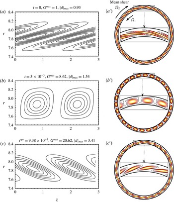
Outside the Rayleigh line, a stratification of the angular momentum exists and the epicyclic frequency is no longer zero. At the initial time, the contours of the kinetic energy associated with the perturbation are oriented against the basic shear, as shown in figure 27(a) in the plane
 $(r,z)$
and in figure 27(
 $a^{\prime }$
) in the plane
 $(r,{\it\theta})$
. These contours will tilt progressively until they almost align with the shear at
 $t=t^{opt}$
, as shown in figure 27(c,
 $c^{\prime }$
).
Optimal perturbation for a Newtonian fluid for
 ${\it\eta}=0.881$
,
 $\mathit{Re}_{1}=101$
,
 $\mathit{Re}_{2}=-1061.2$
with
 $m^{opt}=13$
,
 $k^{opt}=2.176$
. Left: contours of the kinetic energy in the plane (
 $r,z$
) at (a) initial time
 $t=0$
, (b)
 $t\approx t^{opt}/2$
and (c) optimal time
 $t=t^{opt}$
. Right: contours of the kinetic energy in the plane (
 $r,{\it\theta}$
) at
 $(a^{\prime })$
initial time
 $t=0$
,
 $(b^{\prime })~t\approx t^{opt}/2$
and
 $(c^{\prime })$
optimal time
 $t=t^{opt}$
. The quantity
 $d=\partial u^{\prime }/\partial r+u^{\prime }/r+(1/r)\,\partial v^{\prime }/\partial {\it\theta}$
is the 2D divergence on the shear plane.

7.2.2. Purely viscous shear-thinning fluids
In the case of purely viscous shear-thinning fluids, the angular momentum is no longer constant along the Rayleigh line. The optimal perturbation in the whole stable domain of plane (
 $\mathit{Re}_{1},\mathit{Re}_{2}$
) is qualitatively similar to that obtained for a Newtonian fluid outside the Rayleigh line. Further computations show that the evolution of the optimal perturbation with time for shear-thinning fluids with
 ${\it\eta}=0.881$
and
 ${\it\eta}=0.4$
is similar to the Newtonian fluid. However, the optimal perturbation is merely concentrated near the inner wall and more pronounced for a large gap
 ${\it\eta}=0.4$
. Furthermore, the transient growth is reduced with decreasing
 ${\it\eta}$
.
7.2.3. Discussion
Three-dimensional optimal perturbations are initially oriented in the direction opposite to the base flow, then aligned with it at optimal time, e.g. figure 27(c,
 $c^{\prime }$
). The same evolution was observed in a boundary layer flow, when the optimization concerns an initial state characterized by a wavepacket rather than a single wavenumber (Cherubini et al.
Reference Cherubini, Robinet, Bottaro and De Palma2010; Monokrousos et al.
Reference Monokrousos, Akervik, Brandt and Henningson2010). This is in contrast to 2D optimal perturbations, which are oriented transversally to the main shear at the optimal time, as shown by Butler & Farrell (Reference Butler and Farrell1992) for plane Couette and Poiseuille flows. Two-dimensional perturbations, i.e. spanwise-independent perturbations, grow only via the Orr mechanism (Orr Reference Orr1907): a mechanism based on Kelvin’s circulation theorem. The initial contour of the vertical structure shortens as it is tilted by the mean shear. As a consequence, the velocity along the contour has to increase to conserve the initial circulation. In the 3D situation, another mechanism, absent in two dimensions, is active. Indeed, the basic shear vorticity, pointing in the spanwise (here axial) direction, may be stretched due to variations of areas in the shear plane, as was shown by Vitoshkin et al. (Reference Vitoshkin, Heifetz, Gelfgat and Harnik2012) in plane shear flows. These authors pointed out that the interplay between the spanwise vorticity
 $q$
and the planar divergence
 $d$
fields play a dominant role in energy growth. We extended their analysis to the case of Taylor–Couette flow and found that there is (as in the plane shear flow) a mutual growth of
 $d$
and
 $q$
and the maximum is reached at
 $t=t^{opt}$
, i.e. when the perturbation is tilted with respect to the basic shear. Following Vitoshkin et al. (Reference Vitoshkin, Heifetz, Gelfgat and Harnik2012), the role played by the interaction between
 $d$
and
 $q$
is highlighted in the analysis of the energy growth via the Reynolds stress term. For this, a 2D Helmholtz decomposition is performed
 $$\begin{eqnarray}\tilde{\boldsymbol{u}}=\boldsymbol{u}_{d}+\boldsymbol{u}_{q}\quad \text{with }\boldsymbol{u}_{d}=\boldsymbol{{\rm\nabla}}({\it\phi})\text{ and }\boldsymbol{u}_{q}=-\text{rot}({\it\psi}\,\boldsymbol{e}_{z})\end{eqnarray}$$
where
 ${\it\phi}$
and
 ${\it\psi}$
are scalar functions, such that the planar divergence
 $d=\partial u^{\prime }/\partial r+u^{\prime }/r+(1/r)\,\partial v^{\prime }/\partial {\it\theta}$
and the axial vorticity
 $q=(1/r)\partial (rv^{\prime })/\partial r-(1/r)\partial u^{\prime }/\partial {\it\theta}$
satisfy
 $$\begin{eqnarray}d={\it\Delta}_{H}({\it\phi})\quad \text{and}\quad q={\it\Delta}_{H}({\it\psi}),\end{eqnarray}$$
where
 ${\it\Delta}_{H}=\partial ^{2}/\partial r^{2}+(1/r)\partial /\partial r+(1/r^{2})\partial /\partial {\it\theta}^{2}$
is the 2D Laplacian on the shear plane. At the inviscid limit the spatially averaged energy equation is
 $$\begin{eqnarray}\displaystyle \frac{\partial \langle E\rangle }{\partial t} & = & \displaystyle -\mathit{Re}_{1}\langle \dot{{\it\gamma}}_{r{\it\theta}}^{b}\tilde{u} \tilde{v}^{\ast }\rangle \nonumber\\ \displaystyle & = & \displaystyle -\mathit{Re}_{1}\langle \dot{{\it\gamma}}_{r{\it\theta}}^{b}(u_{d}+u_{q})(v_{d}^{\ast }+v_{q}^{\ast })\rangle \nonumber\\ \displaystyle & = & \displaystyle -\mathit{Re}_{1}(\langle \dot{{\it\gamma}}_{r{\it\theta}}^{b}u_{d}v_{d}^{\ast }\rangle +\langle \dot{{\it\gamma}}_{r{\it\theta}}^{b}u_{d}v_{q}^{\ast }\rangle +\langle \dot{{\it\gamma}}_{r{\it\theta}}^{b}u_{q}v_{d}^{\ast }\rangle +\langle \dot{{\it\gamma}}_{r{\it\theta}}^{b}u_{q}v_{q}^{\ast }\rangle ),\end{eqnarray}$$
with
 $E=|\tilde{\boldsymbol{u}}|^{2}/2$
,
 $\boldsymbol{u}_{d}=(u_{d},v_{d},w_{d})$
and
 $\boldsymbol{u}_{q}=(u_{q},v_{q},w_{q})$
.
The first term on the right-hand side of (7.12) is the contribution of the divergent field. The second and the third terms, i.e. mixed
 $q{-}d$
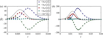
terms, translate the interplay between the planar divergence and the axial vorticity. The fourth term represents the 2D Orr mechanism. The contribution of the different terms as a function of time is shown in figure 28(a) for a Newtonian fluid and figure 28(b) for a power-law fluid. Qualitatively, the evolutions of the different Reynolds stress components are quite similar; however, the amplitudes reached are higher for power-law fluids. For both fluids, the energy growth is initially dominated by the rotational term
 $-\langle \dot{{\it\gamma}}_{r{\it\theta}}^{b}u_{q}v_{q}^{\ast }\rangle$
, i.e. the 2D Orr mechanism. From
 $t\approx t^{opt}/2$
, the vortices are tilted with the shear,
 $-\langle \dot{{\it\gamma}}_{r{\it\theta}}^{b}u_{q}v_{q}^{\ast }\rangle$
becomes negative, i.e. the Orr mechanism contributes to the decay of the energy. The contribution of the planar divergence term is positive, but very small. The contribution of the mixed term
 $d{-}q$
is positive and is at the origin of the increase of
 $E$
when the vortices align with the base shear.
Contribution of the different Reynolds stress components to the energy amplification of a 3D perturbation for
 ${\it\eta}=0.881$
,
 $\mathit{Re}_{1}=101$
and
 $\mathit{Re}_{2}=-1061.2$
. (a) Newtonian fluid,
 $m^{opt}=13$
,
 $k^{opt}=2.176$
and
 $G^{opt}=20.62$
. (b) Power-law fluid
 $n=0.5$
,
 $m^{opt}=11$
,
 $k^{opt}=1.647$
and
 $G^{opt}=88.16$
.

8. Conclusion
In this paper, we performed a 3D linear stability analysis of a circular Couette flow of shear-thinning fluids in both a thin gap (
 ${\it\eta}=0.881$
) and a wide gap (
 ${\it\eta}=0.4$
) between two infinitely coaxial cylinders. Long- and short-time evolutions of the disturbances are investigated. Two rheological models were adopted, the power-law model and the Carreau model, to describe the shear-thinning behaviour of the fluids.
First, we considered the asymptotic evolution at long times. Using a normal-mode approach, an eigenvalue problem was derived and solved with a Chebyshev spectral collocation method. The results show that, for a given
 $\mathit{Re}_{2}$
, the shear-thinning character leads to a decrease of the inner critical Reynolds number
 $\mathit{Re}_{1c}$
, except in the vicinity of
 $\mathit{Re}_{2}=0$
and for a co-rotating regime with a small gap. This reduction is due to an enhancement of the energy exchange between the perturbation and the base flow, which is probably a consequence of the increased shear rate at the inner cylinder wall.
For counter-rotating cylinders, the threshold of the outer Reynolds number,
 $|\mathit{Re}_{2}|$
, at which the critical modes switch from axisymmetric Taylor vortices to spiral vortices increases significantly with increasing shear-thinning effects. The axial wavelength of these spiral vortices is strongly reduced with increasing shear-thinning effects, because of the reduction of the ‘effective gap’ where the Rayleigh’s instability criterion holds.
Second, we studied the transient growth of the perturbation kinetic energy that occurs at short times due to the non-normality of the operators involved in the linearized perturbation equations. A strong increase is observed, up to one order of magnitude for shear-thinning fluids, compared to the Newtonian fluid for given
 $\mathit{Re}_{1}$
and
 $\mathit{Re}_{2}$
.
Features of the optimal perturbation were then determined. We showed that, at large shear Reynolds numbers and for a thin gap, the structure of the optimal perturbation exhibits a large azimuthal wavenumber
 $m^{opt}\approx 12$
and a small axial wavenumber
 $1\leqslant k^{opt}\leqslant 2$
, whereas for a wide gap (
 ${\it\eta}=0.4$
),
 $m^{opt}=2$
and
 $k^{opt}\propto 1$
. It appears that shear-thinning effects have little influence on
 $k^{opt}$
and
 $m^{opt}$
.
-
(i) In the particular case of a Newtonian fluid with
$(\mathit{Re}_{1},\mathit{Re}_{2})$
on the Rayleigh line, the angular momentum is constant and the optimal perturbation consists of a superposition along the axial direction of high and low azimuthal velocity streaks, which evolve towards Taylor vortices via the anti-lift-up mechanism. The optimal energy growth behaves as
$G^{opt}\propto \mathit{Re}^{2}$
. -
(ii) Outside the Rayleigh line, the optimal perturbation, initially oriented against the base shear, tilts until it almost aligns with the shear at
$t=t^{opt}$
. The amplification of the 3D optimal perturbation is analysed in terms of interplay between the planar divergence and the axial vorticity, as suggested by Vitoshkin et al. (Reference Vitoshkin, Heifetz, Gelfgat and Harnik2012). The decomposition of the Reynolds stress in terms of the various contributions from the divergent and the rotational fields indicates that the energy growth is dominated by the mixed terms
$-(u_{d}v_{q}+u_{q}v_{d})\dot{{\it\gamma}}_{r{\it\theta}}^{b}$
, which overwhelm the decaying effect of the Orr mechanism. The numerical results show that the optimal energy growth behaves as
$G^{opt}\propto \mathit{Re}^{2/3}$
, in agreement with Maretzke et al. (Reference Maretzke, Hof and Avila2014).




For shear-thinning fluids, the Rayleigh line should not be distinguished from other situations; the tilting mechanism, described above, applies and the numerical results show that
 $G^{opt}=G_{n=1}^{opt}\exp (-n^{1/3})$
. The transient energy growth is enhanced with increasing shear-thinning effects. Thus, shear thinning promotes the transition to turbulence through the linear superposition of eigenmodes. This tendency was observed in a plane Couette flow (Liu & Liu Reference Liu and Liu2011) and a Hagen–Poiseuille flow (Liu & Liu Reference Liu and Liu2012) of power-law fluids involving another transient growth mechanism.
Acknowledgements
The financial support for this work from the Energy Cell of the french National Center for Scientific Research (CNRS) is gratefully acknowledged.
Appendix A. Operators involved in the linearized perturbation equations
The initial value problem (5.12) reads
 $$\begin{eqnarray}\mathscr{L}\tilde{\boldsymbol{q}}=\mathscr{M}\,\frac{\partial \tilde{\boldsymbol{q}}}{\partial t}.\end{eqnarray}$$
A.1.
$(\tilde{u} ,\tilde{v})$
formulation

In this case,
 $\tilde{\boldsymbol{q}}=(\tilde{u} ,\tilde{v})^{\text{T}}$
and the operators
 $\mathscr{M}$
and
 $\mathscr{L}$
are expressed below
 $$\begin{eqnarray}\displaystyle \mathscr{M} & = & \displaystyle \left(\begin{array}{@{}cc@{}}D\,D_{\ast }-k^{2} & \displaystyle \frac{\text{i}\,m}{r}\,\tilde{D}\\ \displaystyle -\frac{\text{i}\,m}{k^{2}\,r}\,D_{\ast } & \displaystyle 1+\frac{m^{2}}{k^{2}\,r^{2}}\end{array}\right)\end{eqnarray}$$
 $$\begin{eqnarray}\displaystyle \mathscr{L} & = & \displaystyle \mathscr{L}_{I}+\mathscr{L}_{V1}+\mathscr{L}_{V2}+\mathscr{L}_{V3}\end{eqnarray}$$
 $$\begin{eqnarray}\displaystyle \mathscr{L}_{I} & = & \displaystyle \mathit{Re}_{1}\left(\begin{array}{@{}cc@{}}\displaystyle \frac{\text{i}\,m}{r}\,[-(V^{b}\,\widetilde{D}+D\,V^{b})\,D_{\ast }+k^{2}\,V^{b}] & \displaystyle -2\,\frac{k^{2}\,V^{b}}{r}+\frac{m^{2}}{r^{2}}\left(-\frac{2\,V^{b}}{r}+\,D\,V^{b}+\,V^{b}\,D\right)\\ \displaystyle -D_{\ast }\,V^{b}-\frac{m^{2}}{k^{2}\,r^{2}}\,V^{b}\,D_{\ast } & \displaystyle -\frac{\text{i}\,m}{r}\left(1+\frac{m^{2}}{k^{2}\,r^{2}}\right)V^{b}\end{array}\right)\nonumber\\ \displaystyle & & \displaystyle\end{eqnarray}$$
 $$\begin{eqnarray}\displaystyle \mathscr{L}_{V1} & = & \displaystyle {\it\mu}^{b}\left(\begin{array}{@{}cc@{}}(D\,D_{\ast }-k^{2})^{2} & \displaystyle \text{i}\,m\left[\frac{2\,k^{2}}{r^{2}}+D\,{\it\Delta}\frac{1}{r}\left({\it\Delta}-\frac{2D}{r}+\frac{1}{r^{2}}\right)\right]\\ \displaystyle \frac{\text{i}\,m}{r}\left(-\frac{{\rm\Delta}D_{\ast }}{k^{2}}+\frac{2}{r}\right) & \displaystyle D\,D_{\ast }-k^{2}+\frac{m^{2}}{k^{2}\,r^{2}}\,\left({\it\Delta}-\frac{2D}{r}+\frac{1}{r^{2}}-k^{2}\right)\end{array}\right)\end{eqnarray}$$
 $$\begin{eqnarray}\displaystyle \mathscr{L}_{V2} & = & \displaystyle D{\it\mu}^{b}\left(\begin{array}{@{}cc@{}}D^{2}\,D_{\ast }+{\rm\Delta}D_{\ast }-k^{2}\,D & \displaystyle \frac{\text{i}\,m\,}{r}\left({\it\Delta}+D^{2}-\frac{4D}{r}+\frac{3}{r^{2}}\right)\\ \displaystyle -\frac{\text{i}\,m}{k^{2}\,r}\,D\,D_{\ast } & \displaystyle \left(1+\frac{m^{2}}{k^{2}\,r^{2}}\right)\widetilde{D}\end{array}\right)+\,D^{2}{\it\mu}^{b}\left(\begin{array}{@{}cc@{}}k^{2}\,+D\,D_{\ast } & \displaystyle \frac{\text{i}\,m}{r}\widetilde{D}\\ 0 & 0\end{array}\right)\nonumber\\ \displaystyle & & \displaystyle\end{eqnarray}$$
 $$\begin{eqnarray}\displaystyle \mathscr{L}_{V3} & = & \displaystyle ({\it\mu}_{t}-{\it\mu}^{b})\left(\begin{array}{@{}cc@{}}\displaystyle \frac{k^{2}\,m^{2}}{r^{2}} & \displaystyle -\frac{\text{i}\,k^{2}\,m\,\widetilde{D}}{r}\\ \displaystyle \frac{\text{i}\,m\,D_{\ast }}{r} & \displaystyle \left(D\,+\frac{2}{r}\right)\,\widetilde{D}\end{array}\right)+D\,({\it\mu}_{t}-{\it\mu}^{b})\left(\begin{array}{@{}cc@{}}0 & 0\\ \displaystyle \frac{\text{i}\,m}{r} & \widetilde{D}\end{array}\right).\end{eqnarray}$$
A.2.
$(\tilde{u} ,\tilde{w})$
formulation

In this case,
 $\tilde{\boldsymbol{q}}=(\tilde{u} ,\tilde{w})^{\text{T}}$
and the operators
 $\mathscr{M}$
and
 $\mathscr{L}$
are expressed below
 $$\begin{eqnarray}\displaystyle \mathscr{M} & = & \displaystyle \left(\begin{array}{@{}cc@{}}\displaystyle D_{\ast }^{2}+\frac{1}{r}D_{\ast }-\frac{m^{2}}{r^{2}} & \displaystyle \text{i}\,k\,D+\frac{2\,\text{i}\,k}{r}\\ kD_{\ast } & \displaystyle \text{i}\,k^{2}+\frac{\text{i}\,m^{2}}{r^{2}}\end{array}\right)\end{eqnarray}$$
 $$\begin{eqnarray}\displaystyle \mathscr{L} & = & \displaystyle \mathscr{L}_{I}+\mathscr{L}_{V1}+\mathscr{L}_{V2}+\mathscr{L}_{V3}\end{eqnarray}$$
 $$\begin{eqnarray}\displaystyle \mathscr{L}_{I} & = & \displaystyle \mathit{Re}_{1}\left(\begin{array}{@{}cc@{}}\displaystyle \frac{\text{i}\,m}{r^{2}}\left(2\,D\,V^{b}+V^{b}\,D-3\,V^{b}\,D_{\ast }+\frac{m^{2}\,V^{b}}{r}\right) & \displaystyle \frac{3\,k\,m\,V^{b}}{r^{2}}\\ \displaystyle \frac{\text{i}\,k\,m}{r}(D\,V^{b}-V^{b}\,D) & \displaystyle \frac{m}{r}\left(\frac{m^{2}\,V^{b}}{r^{2}}+k^{2}\,V^{b}\right)\end{array}\right)\nonumber\\ \displaystyle & & \displaystyle +\,\mathit{Re}\left(\begin{array}{@{}cc@{}}\displaystyle \frac{\text{i}\,m}{r}\left[-\frac{DV^{b}}{r}+D^{2}V^{b}-V^{b}D\,D_{\ast }\right] & \displaystyle \frac{k\,m}{r}(V^{b}\,D+DV^{b})\\ 0 & 0\end{array}\right)\end{eqnarray}$$
 $$\begin{eqnarray}\displaystyle \mathscr{L}_{V1} & = & \displaystyle {\it\mu}^{b}\left(\begin{array}{@{}cc@{}}\displaystyle -\frac{2\,m^{2}}{r^{4}} & \displaystyle \text{i}\,k\left[\left(\frac{2}{r}+D\right)(D_{\ast }D-k^{2})+\frac{2D_{\ast }D}{r}-\left(\frac{4}{r}+D\right)\frac{m^{2}}{r^{2}}\right]\\ \displaystyle k\,\left({\it\Delta}+\frac{2D}{r}\right)D_{\ast } & \displaystyle \text{i}\,k^{2}\,\left({\it\Delta}+\frac{2\,D}{r}\right)\end{array}\right)\nonumber\\ \displaystyle & & \displaystyle +\,{\it\mu}^{b}\left(\begin{array}{@{}cc@{}}\displaystyle \left(\frac{2}{r}+D\right){\rm\Delta}\,D_{\ast }+\frac{2}{r}\left(D^{2}+\frac{D}{r}\right)\,D_{\ast }-\frac{m^{2}}{r^{2}}\,{\it\Delta}-\frac{m^{2}}{r^{4}} & 0\\ \displaystyle \frac{2\,k\,m^{2}}{r^{3}} & 0\end{array}\right)\end{eqnarray}$$
 $$\begin{eqnarray}\displaystyle \mathscr{L}_{V2} & = & \displaystyle D{\it\mu}^{b}\left(\begin{array}{@{}cc@{}}\displaystyle \frac{2}{r}\,D\,D_{\ast }-\frac{m^{2}}{r^{2}}\left(D-\frac{2}{r}\right) & \displaystyle \text{i}\,k\,\left[{\it\Delta}+\left(\frac{4}{r}+D\right)\,D\right]\\ k\,D\,D_{\ast } & \displaystyle \text{i}\,\left(k^{2}+\frac{m^{2}}{r^{2}}\right)D\end{array}\right)\nonumber\\ \displaystyle & & \displaystyle +\,D{\it\mu}^{b}\left(\begin{array}{@{}cc@{}}\displaystyle \left[\left(D+\frac{2}{r}\right)\,D+{\it\Delta}\right]\,D_{\ast } & 0\\ 0 & 0\end{array}\right)+D^{2}{\it\mu}^{b}\left(\begin{array}{@{}cc@{}}\displaystyle D\,D_{\ast }+\frac{m^{2}}{r^{2}} & \text{i}\,k\,D\\ 0 & 0\end{array}\right)\end{eqnarray}$$
 $$\begin{eqnarray}\displaystyle \mathscr{L}_{V3} & = & \displaystyle ({\it\mu}_{t}-{\it\mu}^{b})\left(\begin{array}{@{}cc@{}}\displaystyle \left[\left(\frac{5}{r}+D\right)\,D+\frac{3}{r^{2}}+\frac{2\,m^{2}}{r^{2}}\right]\,D\,D_{\ast }+\frac{m^{4}}{r^{4}} & \displaystyle \text{i}\,k\,\left[\frac{m^{2}}{r^{2}}+\frac{3}{r^{2}}+\left(\frac{5}{r}+D\right)\,D\right]\,D\\ \displaystyle k\,\left[\left(\frac{3}{r}+D\right)\,D+\frac{m^{2}}{r^{2}}\right]\,D_{\ast } & \displaystyle \text{i}\,k^{2}\,\left(D+\frac{3}{r}\right)\,D\end{array}\right)\nonumber\\ \displaystyle & & \displaystyle +\,D({\it\mu}_{t}-{\it\mu}^{b})\left(\begin{array}{@{}cc@{}}\displaystyle \left(\frac{5}{r}+2\,D\right)\,D\,D_{\ast }+\frac{m^{2}}{r^{2}}\,(D+D_{\ast }) & \displaystyle \text{i}\,k\,\left(\frac{5}{r}+2\,D\right)\,D\\ \displaystyle \frac{k\,m^{2}}{r^{2}}+k\,D\,D_{\ast } & \text{i}\,k^{2}\,D\end{array}\right)\nonumber\\ \displaystyle & & \displaystyle +\,D^{2}({\it\mu}_{t}-{\it\mu}^{b})\left(\begin{array}{@{}cc@{}}\displaystyle D\,D_{\ast }+\frac{m^{2}}{r^{2}} & \text{i}\,k\,D\,\\ 0 & 0\end{array}\right).\end{eqnarray}$$
Appendix B. Demonstration that the eigenvalues for a Newtonian fluid on the Rayleigh line are real
The eigenvalue problem reads
 $$\begin{eqnarray}\mathscr{L}\boldsymbol{q}={\it\sigma}\mathscr{M}\boldsymbol{q},\end{eqnarray}$$
where
 $\boldsymbol{q}=(u,v)^{\text{T}}$
or
 $(u,w)^{\text{T}}$
, depending on the formulation adopted.
For a Newtonian fluid, on the Rayleigh line, the angular momentum of the base flow is constant,
 $\text{d}/\text{d}r(rV^{b})^{2}=0$
, thus
 $$\begin{eqnarray}V^{b}={\displaystyle \frac{a}{r}},\end{eqnarray}$$
where
 $a$
is a constant scalar and
 $$\begin{eqnarray}D_{\ast }V^{b}=DV^{b}+{\displaystyle \frac{V^{b}}{r}}=0.\end{eqnarray}$$
As stressed by Gebhardt & Grossmann (Reference Gebhardt and Grossmann1993), two types of modes exist. The first type corresponds to
 $v\neq 0$
and the second to
 $v=0$
.
If
 $v\neq 0$
then the
 $v$
equation of the (
 $u,v$
) formulation is considered (second line of system (B 1)),
 $$\begin{eqnarray}{\it\sigma}\,v={\it\mu}^{b}\,(D\,D_{\ast }\,v-k^{2}\,v).\end{eqnarray}$$
This equation is multiplied by the complex conjugate of
 $v$
,
 $v^{\ast }$
and integrated over volume
 $\mathscr{V}=2{\rm\pi}^{2}(R_{2}^{2}-R_{1}^{2})/k$
 $$\begin{eqnarray}{\it\sigma}\int _{R_{1}}^{R_{2}}\int _{0}^{2{\rm\pi}}\int _{0}^{2{\rm\pi}/k}\,v\,v^{\ast }\,r\,\text{d}r={\it\mu}^{b}\int _{R_{1}}^{R_{2}}\int _{0}^{2{\rm\pi}}\int _{0}^{2{\rm\pi}/k}\,(D\,D_{\ast }\,v-k^{2}\,v)\,v^{\ast }\,r\,\text{d}r.\end{eqnarray}$$
After integration by parts, this equation becomes
 $$\begin{eqnarray}{\it\sigma}\int _{R_{1}}^{R_{2}}\,v\,v^{\ast }\,r\,\text{d}r=-{\it\mu}^{b}\int _{R_{1}}^{R_{2}}\,[(D_{\ast }\,v)\,(D_{\ast }\,v^{\ast })+k^{2}\,v\,v^{\ast }]\,r\,\text{d}r.\end{eqnarray}$$
If
 $v=0$
then the
 $u$
equation of the (
 $u,v$
) formulation is considered (first line of system (B 1)),
 $$\begin{eqnarray}{\it\sigma}\,(D\,D_{\ast }-k^{2})\,u=\,{\it\mu}^{b}\,(D\,D_{\ast }-k^{2})^{2}\,v.\end{eqnarray}$$
This equation is multiplied by the complex conjugate of
 $u$
,
 $u^{\ast }$
and integrated over a volume
 $\mathscr{V}$
and after integration by parts, we obtain
 $$\begin{eqnarray}-{\it\sigma}\int _{R_{1}}^{R_{2}}\,[(D_{\ast }\,u)\,(D_{\ast }\,u^{\ast })+k^{2}\,u\,u^{\ast }]\,r\,\text{d}r={\it\mu}^{b}\int _{R_{1}}^{R_{2}}\,(D\,D_{\ast }\,u-k^{2}\,u)\,(D\,D_{\ast }\,u^{\ast }-k^{2}\,u^{\ast })\,r\,\text{d}r.\end{eqnarray}$$
For both (B 8) and (B 6), the coefficient of the eigenvalue
 ${\it\sigma}$
and the right-hand side are real and do not depend on
 $\mathit{Re}_{1}$
. Furthermore, the left-hand side coefficient is negative and the right-hand side is positive. The eigenvalue is thus real and negative, and is independent of
 $\mathit{Re}_{1}$
.
Marginal stability curves in the plane (
 $\mathit{Re}_{1w},\mathit{Re}_{2w}$
) for a power-law fluid: (1)
 $n=1$
, Newtonian fluid, (2)
 $n=0.7$
, (3)
 $n=0.5$
, and (4)
 $n=0.3$
. (a)
 ${\it\eta}=0.881$
; (b)
 ${\it\eta}=0.4$
.

Marginal stability curves in the plane (
 $\mathit{Re},R_{{\it\Omega}}$
) for a power-law fluid with
 ${\it\eta}=0.881$
. (1) Newtonian fluid, (2)
 $n=0.7$
, (3)
 $n=0.5$
, and (4)
 $n=0.3$
.

Appendix C. Effect of the viscosity scale on the stabilization/destabilization of shear thinning
We adopt here a definition of the Reynolds numbers based on the viscosity evaluated at the inner wall,
 $\hat{{\it\mu}}^{b}(\hat{R}_{1})$
,
 $$\begin{eqnarray}\mathit{Re}_{(1,2)w}=\frac{\hat{{\it\rho}}\hat{R}_{(1,2)}\hat{{\it\Omega}}_{(1,2)}\hat{d}}{\hat{{\it\mu}}^{b}(\hat{R}_{1})}.\end{eqnarray}$$
Figure 29 shows marginal stability curves in terms of
 $\mathit{Re}_{1w}$
and
 $\mathit{Re}_{2w}$
,
 $$\begin{eqnarray}\mathit{Re}_{1w}=\frac{\hat{{\it\rho}}\hat{R}_{1}\hat{{\it\Omega}}_{1}\hat{d}}{\hat{{\it\mu}}^{b}(\hat{R}_{1})},\quad \mathit{Re}_{2w}=\frac{\hat{{\it\rho}}\hat{R}_{2}\hat{{\it\Omega}}_{2}\hat{d}}{\hat{{\it\mu}}^{b}(\hat{R}_{1})}.\end{eqnarray}$$
It appears that the shear-thinning behaviour has a destabilizing effect for a thin gap
 ${\it\eta}=0.881$
when both cylinders are counter-rotating. However, for a large gap
 ${\it\eta}=0.4$
, stabilization is observed. The opposite effect is found by using as scale the viscosity defined by (2.9). Indeed, for a large gap, when
 $n$
decreases,
 ${\it\mu}^{b}(R_{1})$
decreases more rapidly than
 $\mathit{Re}_{1c}$
; this is why
 $\mathit{Re}_{1cw}=\mathit{Re}_{1c}/{\it\mu}^{b}(R_{1})$
increases with increasing shear-thinning effects. The selection of the viscosity scale may be considered to be simply a matter of choice; however, the conclusions that one reaches by comparing different shear-thinning fluids among themselves and against Newtonian fluids can be radically different from one choice to another.
Appendix D. Marginal stability for a power-law fluid in the plane
$(\mathit{Re},R_{{\it\Omega}})$

Figure 30 shows marginal stability curves for a power-law fluid in the plane (
 $\mathit{Re},R_{{\it\Omega}}$
). For a Newtonian fluid, the marginal stability curve is delimited by the lines
 $R_{{\it\Omega}}=-1$
and
 $R_{{\it\Omega}}=(1-{\it\eta})/{\it\eta}$
.