



1. Introduction
Multiple cylindrical engineering structures closely separated are widely encountered. Typical examples include high-rise buildings, chimney stacks, bridge piers, stays, masts, chemical-reaction towers and offshore platforms. Naturally, it is of practical importance to understand the proximity effect on the fluid dynamics associated with a group of cylindrical structures. There have been a rather large number of investigations on the flow around two cylindrical structures (e.g. Zdravkovich Reference Zdravkovich1977; Igarashi Reference Igarashi1981; Lin, Yang & Rockwell Reference Lin, Yang and Rockwell2002; Zhou & Yiu Reference Zhou and Yiu2006; Sumner Reference Sumner2010; Alam, Zhou & Wang Reference Alam, Zhou and Wang2011), which is the simplest configuration of multiple structures and can be in tandem (or in-line), side-by-side or staggered arrangements. Please refer to Zhou & Alam (Reference Zhou and Alam2016) for a recent compendium of past investigations on this flow. The wake of two in-tandem cylinders involves most of the generic flow features associated with multiple structures, including flow separation, shear layer reattachment, quasi-periodic vortices, vortex impingement and interference between two streets. As such, this flow provides an excellent model for understanding the flow physics of more structures.
Cylindrical structures may be aerodynamically classified into three types based on their cross-sectional shapes. The first is characterized by continuous and finite curvature, e.g. circular and elliptical cylinders (Ota et al. Reference Ota, Nishiyama, Kominami and Sato1986; Derakhshandeh & Alam Reference Derakhshandeh and Alam2019; Shi, Alam & Bai Reference Shi, Alam and Bai2020a; Shi et al. Reference Shi, Alam, Bai and Wang2020b, Reference Shi, Bai, Alam, Ji and Zhu2023), where the flow separation point oscillates over the curved surface. The second features sharp corners of an infinitely large curvature, e.g. square and triangular cylinders (Farhadi, Sedighi & Mohsenzadeh Korayem Reference Farhadi, Sedighi and Mohsenzadeh Korayem2010; Ng et al. Reference Ng, Vo, Hussam and Sheard2016; Alam, Abdelhamid & Sohankar Reference Alam, Abdelhamid and Sohankar2020), where the flow separation point is fixed. The third is a combination of the first two types, such as the D-shaped cylinder and square cylinders with rounded corners (Alam et al. Reference Alam, Zhou and Wang2011). Circular and square cylinders are most representative of the first and second types, respectively, and furthermore are most frequently encountered in engineering.
Past research is mostly focused on the wake of two tandem circular cylinders. When two cylinders are arranged in a tandem configuration, the downstream cylinder is submerged in the wake of the upstream cylinder. The upstream cylinder modifies the incoming flow conditions for the downstream cylinder, while the downstream cylinder may act as a drag reduction device or ‘wake stabilizer’ for the upstream cylinder (Lee & Basu Reference Lee and Basu1997). The two cylinders may behave like one single bluff body or like two independent bodies depending on the separation between them and Reynolds number Re = U ∞d/ν, where U ∞ is the free-stream velocity, d is the characteristic width (i.e. diameter for a circular cylinder and side width for a square cylinder) and ν is the kinematic viscosity of the fluid. The wake is in general classified into three regimes based on the spacing ratio L/d, where L is the distance between the centres of the two cylinders. (e.g. Igarashi Reference Igarashi1981; Zdravkovich Reference Zdravkovich1987; Sumner Reference Sumner2010; Zhou & Alam Reference Zhou and Alam2016). At a small L/d = 1 ~ 1.2–1.8, the two cylinders are so close to each other that the free shear layers separated from the upstream cylinder overshoot the other downstream without any reattachment onto its surface, forming a Kármán vortex street behind the cylinders. This flow is referred to as the extended-body regime. A larger L/d (= 1.2–1.8 ~ 3.4–3.8) leads to the reattachment regime, where the shear layers separating from the upstream cylinder reattach to the downstream cylinder and then roll up, forming vortices and separating alternately from the two sides of the downstream cylinder. With L/d > 3.8, the vortex street is formed both between and behind the cylinders, known as the co-shedding regime. It is worth highlighting that the change from one regime to another depends not only on L/d but also on Re and the turbulence intensity Tu of the incoming flow (Igarashi Reference Igarashi1984; Ljungkrona, Norberg & Sundén Reference Ljungkrona, Norberg and Sundén1991; Xu & Zhou Reference Xu and Zhou2004; Alam Reference Alam2014). Xu & Zhou (Reference Xu and Zhou2004) noted that the reattachment regime may occur for L/d = 2.0 ~ 5.0, depending on Re. They further found that the dependence of Strouhal number St (≡ fsd/U ∞, where fs is the predominant vortex frequency) on Re at 2.0 < L/d < 3.0 was markedly different from that at 3.0 < L/d < 5.0, due to a distinct flow physics between the regimes. The former is linked to a transition from the extended-body to the reattachment regime with increasing Re, while the latter is dictated by a transition from the reattachment to the co-shedding regime. As such, they subdivided the reattachment regime into two, i.e. after- and fore-body reattachments, as schematically shown in figure 1. This subdivision is supported by the distinct flow structure and vortex dynamics in the two sub-regimes (Zhou & Yiu Reference Zhou and Yiu2006, Re = 7 × 10³).
Schematic of four distinct flow structures around two tandem circular cylinders (Zhou & Yiu Reference Zhou and Yiu2006): (a) extended body, (b) after-body reattachment, (c) fore-body reattachment and (d) co-shedding.

The flow around two in-line square cylinders has received much less attention than its counterpart of circular cylinders. Attempt has been made to classify this flow. Sakamoto, Hainu & Obata (Reference Sakamoto, Hainu and Obata1987) measured the fluctuating pressures on two tandem square cylinders with a cylinder aspect ratio (length/d) of 9.5 and divided the flow into three regions based on the dependence of St on L/d at Re = 2.76 × 10⁴. In region 1 (L/d ≤ 4), vortices were observed only behind the downstream cylinder. In region 2 (L/d = 4 ~ 28), vortex shedding from the downstream cylinder was synchronized with that from the upstream. At L/d > 28, referred to as region 3, the vortex streets generated by each cylinder were essentially independent of each other. In their further study, Sakamoto & Haniu (Reference Sakamoto and Haniu1988) presented the St–L/d relationship for different turbulent intensities at Re = 3.32 × 10⁴ and reported a bistable phenomenon where the shear layer separated from the upstream cylinder switched from reattachment on the downstream cylinder to rollup, forming vortices in the gap between the cylinders. Du et al. (2022) conducted large-eddy simulations at Re = 8 × 10⁴ and revealed that the extreme pressures on two tandem square cylinders are driven by vortices such as the gap vortex, wall vortex and corner vortex. Based on PIV (particle image velocimetry) measurement at Re = 5.3 × 10³–1.6 × 10⁴, Kim et al. (Reference Kim, Kim, Yoon and Lee2008) identified two markedly distinct flow structures including reattachment and co-shedding flows at L/d ≤ 3 and L/d ≥ 3.5, respectively. They found that Re produced a significant effect on the fluctuating spanwise velocities but not on the streamwise velocities in the wake. Zhao et al. (Reference Zhao, Cheng, Zhang and Hu2016) observed a transition from the reattachment to co-shedding regime at L/d ≈ 4 in their numerical data at Re = 100. Both drag and lift forces on both cylinders were smaller in the reattachment regime than in the co-shedding regime. Choi, Jang & Yang (Reference Choi, Jang and Yang2012) classified the flow of Re = 100–500 into the extended-body (1.8 ≤ L/d ≤ 2.1), reattachment (2.2 ≤ L/d ≤ 4.5) and co-shedding (L/d > 4.5) regimes. Using Floquet stability analysis, they identified the onset of the secondary instability that triggered the transition from two- to three-dimensional flows. The transition from one flow state to another is also studied. Based on their experimental data, Yen, San & Chuang (Reference Yen, San and Chuang2008) found that the transition between the reattachment and co-shedding flows reduced from L/d = 4.6 to 2.5 when Re was increased from 100 to 1300. Sohankar (Reference Sohankar2014) observed numerically a hysteresis in the L/d range of the transition when L/d was progressively increased or decreased. This hysteresis produced discontinuities in aerodynamic forces and flow structures over a certain range of L/d. The L/d range where the hysteresis occurred was 2.25–3.25 for Re = 2.7 × 10³ and 1.5–2.5 for Re = 2 × 10⁴. A similar observation was made by Sobczyk et al. (Reference Sobczyk, Wodziak, Gnatowska, Stempka and Niegodajew2018) for L/d = 2.0–9.0 and Re = 4.1 × 10³–3.29 × 10⁴. Rastan & Alam (Reference Rastan and Alam2021) investigated numerically the wake of two tandem cylinders, including both circular and square cylinders. For Re < 500, their focus was on the effects of Re and L/d (≤ 10) on steady–unsteady flow transitions and flow classification. They found that the flow transition from steady to unsteady occurred at a higher Re than in an isolated cylinder wake. As such, the transition from two- to three-dimensional vortex shedding was postponed in the reattachment regime but advanced in the co-shedding regime. It is worth pointing out that flow at such a low Re range is very different from that of higher Re, say above 103 (Zdravkovich Reference Zdravkovich1997), that is, the findings such as the flow classification of the former cannot be used to predict the latter. Rastan & Alam (Reference Rastan and Alam2021) also studied the flow of Re > 500 based on Sohankar's (Reference Sohankar2014) LES (large-eddy simulation) data, which was far from a systematic approach. The examined L/d was limited to 2 and above, covering only the reattachment and co-shedding regimes, with a focus on the hysteresis phenomenon between the two regimes. The flow in each regime was not well characterized.
In spite of numerous previous investigations, this flow has never been systematically studied and many of its important aspects remain a mystery. For example, since the flow separation point oscillates in a non-stationary fashion on a circular cylinder but is fixed on a square cylinder, one may naturally wonder how the wake of two tandem square cylinders differs from its circular cylinder counterpart. How would this difference in flow separation affect the flow classification and the dependence of St on L/d? The wake of an isolated square cylinder depends weakly on Re, e.g. with an almost constant St ≈ 0.135 (e.g. Vickery Reference Vickery1966), due to the fixed flow separation point. Is this the case for the two tandem square cylinder wake? If not, how does St depend on Re? Two different bistable phenomena have been identified in the wake of two tandem circular cylinders (Xu & Zhou Reference Xu and Zhou2004). Could we expect the same if the circular cylinders are replaced by square cylinders? Sakamoto et al. (Reference Sakamoto, Hainu and Obata1987) proposed a flow classification based on the experimental data of small aspect ratio cylinders. Is this classification valid for long cylinders?
This work aims to perform a systematic study and gain a relatively thorough understanding of the flow structure and the dependence of St on L/d and Re in the turbulent wake of two tandem square cylinders, including the classification of different regimes, with a view to addressing the issues raised above. The L/d range examined is from 1.0 to 5.0 and Re from 2.8 × 10³ to 2.8 × 10⁴. The hot-wire, laser-induced fluorescence (LIF) flow visualization and surface pressure scanning techniques are used to measure the fluctuating streamwise velocity and hence St, the flow structure and the fluid forces, respectively. The dependence of the flow on Re is discussed in detail.
2. Experimental details
2.1. Strouhal number measurements
Hot-wire measurements were conducted in a closed-circuit wind tunnel with a square test section (0.6 m × 0.6 m) of 2.4 m length. The wind speed in the test section is from 1.5 to 50 m s−1. The free-stream velocity was measured using a Pitot-static tube connected to a Furness micro-manometer (FCO 510, Furness Controls Ltd. Bexhill, UK). The experimental uncertainty in the measurement of U ∞ is estimated to be ±1.0 % and the longitudinal turbulent intensity Tu is 0.13 % in the absence of any cylinders. Two identical aluminium square cylinders of d = 19.1 mm, placed in tandem with the upstream cylinder mounted at 0.2 m downstream of the exit plane of the contraction, were installed perpendicularly in the midplane and spanned the full height of the test section, resulting in a maximum blockage of 3.18 % and an aspect ratio of 31.6. The blockage ratio was small enough and no correction was made for measurements (West & Apelt Reference West and Apelt1982), while the aspect ratio was considered to be adequately large to neglect the end effect of the cylinders.
Two Cartesian coordinate systems, (x-O-y) and (x′-O′-y′), are defined such that the origins O and O′ are at the centres of the upstream and downstream cylinders, respectively, with the x- or x′-axis and the y- or y′-axis along the streamwise and lateral directions, respectively. Two hot-wire probes (55P01, Dantec), HT1 and HT2, placed at (x*, y*) = (1.5, 1.5) and (L/d + 1.5, −1.5), respectively, were used to measure the streamwise fluctuating velocities (u 1 and u 2), which provided the information on the vortex shedding from the upstream and downstream cylinders, respectively (please refer to figure 2). The superscript asterisk in this paper denotes normalization by d and/or U ∞. The sensing element of the hot-wire was made of 0.5 μm tungsten wire, approximately 1.25 mm in length, and was connected to constant temperature anemometers (Dantec Streamline) operated at an overheat ratio of 1.8. The signals from the wires were low-pass filtered at a cutoff frequency of 1 kHz and then digitized at a sampling frequency fsampling of 2 kHz on a personal computer using a 16-channel A/D board (NI PCI-6143). The sampling duration was 60 s for each combination of L/d and Re. The hot-wire was not calibrated since the measured u1 and u2 are used only to determine St. The St is determined from the power spectral density function Eu of the u signal, and Eu is calculated from a fast Fourier transform (FFT) algorithm. The FFT window size Nw is 4096. The frequency resolution Δƒ (= fsampling/Nw) in the spectral analysis (Zhou et al. Reference Zhou, Du, Mi and Wang2012) is 0.49 Hz. The St behind an isolated cylinder was also measured to set a benchmark for comparison. Measurements were made for L/d = 1.0 ~ 5.0 and Re = 2.8 × 10³ ~ 2.8 × 10⁴.
Experimental arrangement and definitions of symbols. The parameter L is the spacing between the cylinder centres, and d is the side width of a square cylinder. The hot-wire probes are placed at x* (= x/d) = 1.5, L/d + 1.5 and y* (= y/d) = ±1.5.

2.2. Flow structure measurement
A Dantec high-frequency PIV system (Litron LDY 304-PIV, Nd:YLF) was used to measure the flow in the (x, y) plane. The flow was seeded with particles approximately 1 μm in diameter, generated from paraffin oil using a TSI 9307-6 particle generator. Flow illumination was provided by two pulsed laser sources of 527 nm wavelength, each with a maximum power of 30 mJ per pulse. The interval between two successive pulses was 75 μs. One charge-coupled device camera (Phantom V641, double frames, with a resolution of 2560 × 1600 pixels) was used to capture particle images. An interrogation window of 32 × 32 pixels was applied for image processing with a 50 % overlap in both the x and y directions. A total of 1000 images were captured for each flow configuration, i.e. one combination of L/d and Re, which is considered to be adequate for the root-mean-square values  $u_{rms}^\ast $ of streamwise velocities to be converged. As demonstrated by Alam et al. (Reference Alam, Zhou and Wang2011), the maximum
 $u_{rms}^\ast $ in the wake of an isolated single cylinder converged to its asymptotic value, with a maximum departure of 2.8 %, once the number of images reached 500.
The same PIV system was also used for LIF flow visualization. The four surfaces of each cylinder were painted black to minimize reflection noise. Note that the laser source was placed above the cylinders, which were not transparent, thus partially blocking illumination below the cylinders. This should not adversely affect the capturing of the flow structure given symmetric or anti-symmetric flow about the x-axis (Zhou & Yiu Reference Zhou and Yiu2006). Seven pinholes in a row, each 1 mm in diameter, with a 1.5 mm centre-to-centre distance between two adjacent pinholes, were drilled on the midspan front surface of the upstream cylinder. The first and seventh holes were 1.5 mm away from the lower and upper edges of the cylinder, respectively. Since the cylinder wall was 1 mm in thickness, the distance between the hole centre and the cylinder edge should not be less than 1.5 mm. To measure pressure as close to the cylinder edge as possible, the holes were made 1.5 mm away from the lower or upper edge. Smoke was released from the pinholes to seed the flow. A total of 500 images was recorded for each combination of Re and L/d, although representative results only at Re = 1.3 × 10⁴ and L/d = 1.2, 1.4, 2.0, 2.6, 2.8 and 4.0 are presented in this paper.
2.3. Surface pressure, time-averaged and fluctuating drag and lift measurements
Surface pressure distributions around the two square cylinders were measured at L/d = 1.1 ~ 5.0 with an increment of 0.1 at a representative Re = 1.3 × 10⁴. Each cylinder was furnished with one row of 24 pressure taps (6 taps on each surface) near the midspan. The centre-to-centre distance between two adjacent taps was 3.8 mm. Each tap was offset by 1.5 mm spanwise from its preceding one to minimize possible interference between them. The taps were connected to a pressure scanner (ESP-32HD, 32 ports, with a measurement range of ±1 KPa and a resolution of ±1.5 Pa) through the tubes of 0.8 mm inner diameter. The scanner was placed outside the test section of the wind tunnel, very close to the cylinder ends in order to improve the signal response. The pressure signals were sampled at a rate of 650 Hz to a data acquisition unit (DTC Initium) before being sent via an ethernet cable and stored in a computer. The data record duration was 60 s. The surface pressure around an isolated cylinder was also measured to set a benchmark and validate our results. Integrating the simultaneously captured pressures at 24 pressure taps around a cylinder leads to the time-averaged drag coefficient  ${\bar{C}_D}$ and fluctuating drag and lift coefficients
 ${C^{\prime}_D}$ and
 ${C^{\prime}_L}$. In this paper, overbar and superscript prime denote time-averaged and root-mean-square values, respectively.
2.4. Surface-oil-flow visualization
A surface-oil-flow visualization experiment is employed to capture the mean shear stress pattern, including various singular points, e.g. stagnation, reattachment, separation, etc. (Younis, Alam & Zhou Reference Younis, Alam and Zhou2016; Alam et al. Reference Alam, Rastan, Wang and Zhou2022). The surfaces of the two cylinders were firstly sprayed with black paint as a background, and then a solution of silicone oil (100 cs), titanium dioxide, oleic acid and kerosene with a ratio of 4:1:2:2 in weight was painted onto the surfaces. The cylinders were thereupon installed in the test section of the wind tunnel, and the solution was distributed on the cylinder surface after at least 20 min of exposure to uniform incident flow. The photographs of the solution distributions on the cylinder surfaces were captured by a digital camera with a resolution of 3024 × 4032 pixels. Surface-oil-flow visualizations were performed at the same Reynolds number as the measurements of fluid forces, Strouhal numbers and pressures. The experimental uncertainty in the positions of flow separation or reattachment obtained from surface-oil-film visualization was estimated to be ±0.01d based on the camera resolution.
3. Flow classifications
Flow around two tandem square cylinders may change greatly with L/d and may be classified based on the flow structure captured from the PIV and flow visualization data, as well as the dependence on L/d of St,  ${\bar{C}_D}$,
 ${C^{\prime}_D}$ and
 ${C^{\prime}_L}$. Figure 3 presents the variation in St with L/d (=1.0 ~ 5.0) at Re = 4.5 × 10³, 1.3 × 10⁴ and 2.8 × 10⁴. The data from Sakamoto & Haniu (Reference Sakamoto and Haniu1988) at Re = 3.32 × 10⁴ and Liu & Chen (Reference Liu and Chen2002) at Re = 1.6 × 10⁴ are also included. It is worth commenting that the present vortex-shedding frequencies detected between and behind the two cylinders are in general the same for the L/d range examined (e.g. Armstrong, Barnes & Grant Reference Armstrong, Barnes and Grant1987; Alam & Sakamoto Reference Alam and Sakamoto2005). That is, the shear layer or convected vortices from the upstream cylinder may act to trigger vortex shedding from the downstream cylinder, resulting in a single vortex-shedding frequency. The present St data agree qualitatively with Sakamoto & Haniu (Reference Sakamoto and Haniu1988) and Liu & Chen (Reference Liu and Chen2002). However, there is a deviation in the critical L/d where flow changes from reattachment to co-shedding and St drops sharply. This critical L/d range is presently at 2.7 ~ 3.3, depending on Re, but is 4.0 based on Sakamoto & Haniu (Reference Sakamoto and Haniu1988) and 2.5 based on Liu & Chen (Reference Liu and Chen2002). The discrepancy between Sakamoto & Haniu (Reference Sakamoto and Haniu1988) and ours may be ascribed to a difference in experimental conditions such as Re, aspect ratio, blockage ratio and turbulence intensity Tu (table 1). The critical spacing is sensitive to Tu, and the higher the Tu, the smaller the critical spacing (Sakamoto & Haniu Reference Sakamoto and Haniu1988). Liu & Chen's (Reference Liu and Chen2002) St values are higher in the co-shedding regime but lower in the reattachment regime than the present measurements at Re = 1.3 × 10⁴. The difference arises from the fact that their Tu (= 0.5 %) is larger than ours (Tu = 0.13 %). A larger Tu gives rise to a rise in St in the co-shedding regime but a drop in St in the reattachment regime (Sakamoto & Haniu Reference Sakamoto and Haniu1988). The critical L/d is presently 3.0 ~ 3.2 at Re = 4.5 × 10³ (cylinder aspect ratio = 31.6; blockage ratio = 3.18 %), very close to Kim et al.'s (Reference Kim, Kim, Yoon and Lee2008) measurement (3.5) at Re = 5.3 × 10³ (cylinder aspect ratio = 15; blockage ratio = 6.6 %). An aspect ratio larger than 10 produces a negligible effect on forces and St (Norberg Reference Norberg1994). So does the blockage if less than 6 % (West & Apelt Reference West and Apelt1982) and could have a very small effect if between 6 % and 7.5 % (Mondal & Alam Reference Mondal and Alam2023). The results are comparable between Kim et al.'s (Reference Kim, Kim, Yoon and Lee2008) and the present study. This agreement provides confidence in the present St data.
Variation in Strouhal number St with spacing ratio L/d for Re = 4.5 × 10³–2.8 × 10⁴ in four regimes: regime 1 (extended body), 1.0 ≤ L/d ≤ 1.5; regime 2 (reattachment), 1.5 < L/d < 2.8; regime 3 (transition), 2.8 ≤ L/d ≤ 2.9; regime 4 (co-shedding), L/d > 2.9 at Re = 1.3 × 10⁴. Red coloured symbols indicate the occurrence of two flow states, as indicated by two distinct St values.

Comparison in the characteristic flow parameters between the present and previous data; Re, Reynolds number; L/d, cylinder spacing ratio; l/d, aspect ratio; Tu, longitudinal turbulent intensity; CTA, constant temperature anemometry.

A close examination of the St–L/d relationship in figure 3 unveils four distinct regions in the variation of St with L/d. For 1.0 ≤ L/d ≤ 1.5 ~ 2.0, St rises rapidly with increasing L/d. Then St declines until L/d = 2.6–2.9, followed by a small rise. From L/d = 2.7 to 3.3, St experiences a sudden sharp drop. Once L/d ≥ 3.0 ~ 3.3, St exhibits a gradual rise. In fact, the spectral and flow visualization data point to distinct flow structures from one region to another. The four regions are referred to as the extended-body, reattachment, transition and co-shedding regimes. Note that the exact range of L/d for each regime depends on Re. For example, the transition regime corresponds to L/d = 3.0 ~ 3.2, 2.8 ~ 2.9 and 2.7 ~ 2.9 for Re = 4.5 × 10³, 1.3 × 10⁴ and 2.8 × 10⁴, respectively. This flow classification is made based on multiple flow aspects (the behaviours of the shear layer, vortex shedding from single or both cylinders and how St varies with L/d, as will be discussed in detail in the following subsections), unlike that proposed by Sakamoto & Haniu (Reference Sakamoto and Haniu1988), which was based on whether both cylinders generated vortex streets and whether the streets were independent of each other.
3.1. Extended-body regime
At a small gap, two square cylinders act like one single rectangular cylinder or extended body (Sakamoto et al. Reference Sakamoto, Hainu and Obata1987; Sakamoto & Haniu Reference Sakamoto and Haniu1988; Alam et al. Reference Alam, Rastan, Wang and Zhou2022), and an increase in L/d implies a longer after body, which acts to reduce the wake width w* and shear layer curvature, causing an increased St (Otsuki et al. Reference Otsuki, Washizu, Tomizawa and Ohya1974; Liu & Chen Reference Liu and Chen2002). From a different perspective, the increased L/d is equivalent to an increased ratio, from 2 to 3, of the longitudinal to lateral width of the ‘rectangular’ cylinder, again leading to a larger St (Okajima Reference Okajima1982). As such, St rises rather rapidly, e.g. from 0.086 at L/d = 1.0 to its maximum 0.142 at L/d = 1.5 for Re = 1.3 × 10⁴ (figure 3). The flow characteristics around two tandem cylinders indeed exhibit many similarities to those around a single square cylinder. Bai & Alam (Reference Bai and Alam2018) noted that, for a single square cylinder, the position of transition to turbulence significantly shifts toward the flow separation point when Re is increased from 103 to 104, but insignificantly for Re = 104–105. The shift led to a contracted vortex formation length. Presently, the extended-body regime shrinks from Re = 4500 to 13 000 (figure 3), which is linked to the gradual shift in the transition to turbulence toward the flow separation point. The value of Eu displays one prominent peak at St = 0.086 for L/d = 1.0 (figure 4) and St = 0.118 for L/d = 1.2 (figure 5a). Additional peaks are discernible at the second and third harmonics of St. Figure 5(b) illustrates the flow structure captured from flow visualization in this regime. The shear layers separating from the leading edge of the upstream cylinder roll up behind the downstream cylinder. There is no vortex shedding in the gap between the two cylinders.
Power spectral density function Eu of streamwise velocity u measured by the moveable hot-wires HT1 and HT2. Here, L/d = 1.0, Re = 1.3 × 10⁴.

(a) Power spectral density function Eu of streamwise velocity u measured by the moveable hot-wires HT1 and HT2; (b) image of typical flow structure from smoke visualization. Here, L/d = 1.2, Re = 1.3 × 10⁴.

3.2. Reattachment regime
In this regime, the shear layers separating from the upstream cylinder may reattach to the side surfaces of the downstream one and then separate again from the trailing edges of the cylinder to roll up periodically (Sakamoto & Haniu Reference Sakamoto and Haniu1988). The value of Eu displays one pronounced peak (figure 6a), indicating the occurrence of a single vortex-shedding frequency, and St drops initially rather quickly with increasing L/d (figure 3).
(a) Power spectral density function Eu of streamwise velocity u measured from the moveable hot-wires HT1 and HT2; (b) image of typical flow structure from smoke visualization. Here, L/d = 2.0, Re = 1.3 × 10⁴.

At L/d = 1.5, where the extended-body regime changes to the reattachment regime, the shear layer may reattach to the trailing edge of the downstream cylinder. A comparison in the flow visualization photographs between L/d = 2.0 and 2.6 reveals that the reattachment position shifts toward the leading edge with increasing L/d (figures 6b and 7b). This position influences the shear layer velocity, wake width w*, formation length  $L_f^\ast $, etc. (Wang, Alam & Zhou Reference Wang, Alam and Zhou2018), thus producing a great impact upon St. For example, the shear layer will be subjected to much less obstruction if reattaching near the trailing edge (figure 6b) than near the leading edge (figure 7b). The reverse flow in the gap between the cylinders is thus stronger at L/d = 2.6 than at L/d = 2.0 (figures 6b and 7b). The shear layer instability frequency fsl is inversely proportional to the shear layer thickness in the case of a single circular cylinder (Bauer Reference Bauer1961; Gerrard Reference Gerrard1966; Monkewitz & Nguyen Reference Monkewitz and Nguyen1987; Williamson & Brown Reference Williamson and Brown1998). Based on the data in the literature and their own measurements, Prasad & Williamson (Reference Prasad and Williamson1997) proposed an empirical correlation between Re and fsl for a single circular cylinder wake, namely, fsl/fs = 0.0235 ⋅ Re 0.67. Given a fixed Re, a thick shear layer corresponds to a lower fsl and hence a decreasing fs. An increase in L/d may provide more room for the reattached shear layer to develop before rolling up, implying a thicker layer when separating and hence a lower St. Liu & Chen (Reference Liu and Chen2002) also reported that an increase in L/d in the reattachment regime caused St to decrease, suggesting a wider wake width.
(a) Power spectral density function Eu of streamwise velocity u measured from the moveable hot-wires HT1 and HT2; (b) image of typical flow structure from smoke visualization. Here, L/d = 2.6, Re = 1.3 × 10⁴.

Note a broadband bump of relatively high frequencies (f* > 0.4) in Eu measured from hot-wire 1 (figures 6a and 7a), which is probably due to the instability or Kelvin–Helmholtz vortices of the shear layers separating from the upstream cylinder (figures 6b and 7b). This bump is appreciably stronger for L/d = 2.6 than for L/d = 2.0, suggesting that the reattachment incurs stronger shear layer instability near the leading edge (figure 7b) than near the trailing edge (figure 6b).
3.3. Transition regime
The transition involves a change in the flow structure from reattachment to co-shedding or vice versa, and naturally two distinct St values. The higher St corresponds to the reattachment regime, and the lower to the co-shedding (figure 8b). The L/d range where the transition takes place depends on Re, 3.0 ~ 3.2 for Re = 4.5 × 10³, 2.8 ~ 2.9 for Re = 1.3 × 10⁴ and 2.7 ~ 2.9 for Re = 2.8 × 10⁴. In this regime (e.g. L/d = 2.8, Re = 1.3 × 10⁴), the intermittent occurrence of both flow states is captured in the time histories of u1 and u2 from HT1 and HT2, respectively (figure 8a). Both signals are characterized by small- and large-amplitude fluctuations, corresponding to the reattachment and co-shedding flow structures, respectively (figure 8a). The value of Eu, calculated from u1 or u2, shows two prominent peaks at St = 0.100 and 0.131 (figure 8b). The peak is less pronounced at St = 0.131 than at St = 0.100. The higher St results from vortex shedding when reattachment occurs and the lower from vortex shedding when co-shedding takes place. It seems plausible that the vortices associated with the co-shedding state are characterized by a larger strength than those formed in the reattachment state. Figure 8(c,d) shows the corresponding flow structures in the two states. In the reattachment case, the gap shear layer reattaches on the leading edge of the downstream cylinder and splits into two, partly moving into the gap between the cylinders and partly flowing over the side surface, and then rolls up to form vortices behind the downstream cylinder (figure 8c). In the co-shedding case, the shear layer appears to roll up entirely in the gap between the cylinders, forming the gap vortices (figure 8d). As seen in figure 8(c,d), the curvature of the gap shear layer appears larger in the co-shedding case than in the reattachment flow, resulting in a smaller St in the latter case (Nakaguchi, Hasimot & Muto Reference Nakaguchi, Hasimot and Muto1968; Alam et al. Reference Alam, Zhou and Wang2011). Furthermore, being obstructed by the downstream cylinder, the gap vortices are convected at a small velocity, also contributing to a smaller St (figure 8b). Sakamoto & Haniu (Reference Sakamoto and Haniu1988) observed at Re = 3.32 × 10⁴ the bistable flow involving reattachment and co-shedding at L/d = 4.0 for their smallest Tu (= 0.19 %) examined. Their transition took place at a considerably larger L/d than the present L/d. This difference is not surprising since their blockage ratio, inter alia, reached 9.8 %, considerably larger than the present 3.18 %.
(a) Time histories of streamwise velocity u from hot-wires HT1 and HT2; (b) power spectral density function Eu of streamwise velocity u and measured from the moveable hot-wires HT1 and HT2; (c,d) images of typical flow structures from smoke visualization. Here, L/d = 2.8, Re = 1.3 × 10⁴.

3.4. Co-shedding regime
In this regime, the quasi-periodical vortices are generated both between and behind the cylinders at the same frequency (figure 9). The value of St rises slowly with increasing L/d, which is linked to the gradually diminishing effect of the downstream cylinder on the upstream cylinder, and eventually approaches that in an isolated cylinder wake (Sto = 0.132). One may expect a different vortex-shedding frequency in the gap between the cylinders from that behind because of the very different initial conditions of incident flow. However, the former may trigger the latter, producing a ‘lock-in’ phenomenon (Alam & Sakamoto Reference Alam and Sakamoto2005).
(a) Power spectral density function Eu of streamwise velocity u measured from the moveable hot-wires HT1 and HT2; (b) image of typical flow structure from smoke visualization. Here, L/d = 4.0, Re = 1.3 × 10⁴.

4. Flow structures
4.1. Near-wake characteristic parameters
The near wake of a cylinder is characterized by the wake width w* and vortex formation length  $L_f^\ast $, which can be determined from the distribution of
 $u_{rms}^\ast $. Figure 10 presents the iso-contours of PIV-measured
 $u_{rms}^\ast $ (Re = 1.3 × 10⁴) in the wake for the extended-body (L/d = 1.2, 1.4) and reattachment (L/d = 1.8, 2.2, 2.4 and 2.7) regimes. Two maxima occur rather symmetrically about y* = 0, which are frequently considered to be the mean position where the shear layer rollup takes place (Bloor Reference Bloor1964; Gerrard Reference Gerrard1966). The maximum
 $u_{rms}^\ast $ declines from 0.24 to 0.22 when L/d increases from 1.2 to 1.4 in the extended-body regime but remains almost constant, at approximately 0.2, in the reattachment regime from L/d = 1.8–2.4 before dropping further to 0.18 from L/d = 2.4 to 2.7. The observation suggests that the vortices formed become weaker in strength from the extended-body regime to the reattachment regime. Compared with the extended-body regime at L/d = 1.4, the location of the maximum
 $u_{rms}^\ast $ changes a little for L/d = 1.8–2.4 in the reattachment regime but shifts appreciably downstream at L/d = 2.7. This location is correlated with the base pressure of the downstream cylinder, as will be discussed later. As L/d is increased to 3.2 (co-shedding flow), the maximum
 $u_{rms}^\ast $ rises sharply to 0.3, and its position shifts toward the cylinder base, indicating stronger vortex shedding when the flow changes from the reattachment to co-shedding regime. An increase in L/d in the co-shedding regime, e.g. from 3.2 to 4.2, leads to a decrease in the maximum
 $u_{rms}^\ast $ to 0.24.
Iso-contours of the root mean square streamwise velocity  $u_{rms}^\ast = {u_{rms}}/{U_\infty }$ for (a) L/d = 1.2, (b) L/d = 1.4, (c) L/d = 1.8, (d) L/d = 2.2, (e) L/d = 2.4, (f) L/d = 2.7, (g) L/d = 3.2 and (h) L/d = 4.2. Re = 1.3 × 10⁴. The contour increment is 0.02.

The wake width w* can be defined as the transverse distance between the two maximum  $u_{rms}^\ast $ values where the two shear layers roll up to form vortices (Griffin & Ramberg Reference Griffin and Ramberg1974; Roshko Reference Roshko1993). By the same token, following Bloor (Reference Bloor1964) and Gerrard (Reference Gerrard1966), we may define the vortex formation length Lf by the streamwise distance from the downstream cylinder base to the
 $u_{rms}^\ast $ maximum. The variations in w* and
 $L_f^\ast $, along with St, with L/d are presented in figure 11. With increasing L/d, the rise in St in the extended regime is accompanied by a decrease in w*, while the decrease in St from L/d = 1.5 to 2.5 in the reattachment regime is associated with an increase in w*. A further increase in L/d from 2.5 to 2.7 in the reattachment regime results in a decline in w* but a rise in St. With the flow changing from reattachment (L/d = 2.7) to co-shedding (L/d = 3.2), the sharp drop in St is accompanied by a rise in w* from 1.13 to 1.36. The w* gradually decreases in the co-shedding regime, reaching 1.2 at L/d = 4.2. Overall, St is inversely linked with w*. It has been well established in a single cylinder wake that, for a fixed Re, the smaller the w*, the higher the St (Bearman & Trueman Reference Bearman and Trueman1972; Griffin & Ramberg Reference Griffin and Ramberg1974). It seems plausible that this conclusion is also valid for a two-cylinder system. The variation in
 $L_f^\ast $ with L/d is, however, different from that in w*. The
 $L_f^\ast $ contracts from 1.65 at L/d = 1.2 to 1.08 at L/d = 1.4 in the extended-body regime and remains almost unchanged in the reattachment regime, albeit displaying a rise from L/d = 2.4 to 2.7. The transition regime is characterized by a drastic drop in
 $L_f^\ast $ from 1.04 at L/d = 2.7 to 0.38 at L/d = 3.2. The value of
 $L_f^\ast $ remains more or less constant in the co-shedding regime. The observation suggests that St is more closely correlated with or influenced by w* than by
 $L_f^\ast $.
Dependence on cylinder spacing ratio L/d of (a) wake width w* and Strouhal number St and (b) vortex formation length  $L_f^\ast $ from the centre of upstream cylinder at Re = 1.3 × 10⁴.

4.2. Velocity field in the wake
It is important to understand the shear layer development, vortex shedding and flow structure (both instantaneous and time averaged) behind the cylinders in the different flow regimes. As such, we present the time-averaged sectional streamlines (referred to as streamlines hereinafter for simplicity), superimposed with the iso-contours of time-averaged streamwise velocity  ${\bar{U}^\ast }$ or spanwise vorticity
 $\bar{\omega }_z^\ast $ in figures 12(a), 13(a) and 14(a), along with the phase-averaged streamlines, superimposed with phase-averaged vorticity
 $\langle \omega _z^\ast \rangle$ in figures 12(b), 13(b) and 14(b). The phase-averaged streamlines are viewed on a reference frame moving at the vortex convection velocity
 $\langle U_c^\ast \rangle$, estimated as the streamwise displacement of the vortex between two successive PIV snapshots divided by the corresponding time interval. One thousand time-resolved PIV snapshots were captured over a duration of 1 s, out of which the time histories of u and v may be extracted. As in Chen et al. (Reference Chen, Zhou, Zhou and Antonia2016), a fourth-order Butterworth filter, centred at the vortex-shedding frequency, was used to filter the signal of thus obtained v at (x*, y*) = (L/d + 1.5, −1.5), producing a sinusoidal signal. This signal was used as the reference signal to determine the phase. In the phase-averaging process, approximately 20 data points are available for each phase.
(a) Time-averaged streamlines superimposed with the normalized iso-contours: (ai) time-mean streamwise velocity  ${\bar{U}^\ast }$, (aii) time-mean spanwise vorticity
 $\bar{\omega }_z^\ast $, (aiii) flow structure sketch; (b) phase-averaged streamlines after subtracting convection velocity, superimposed with phase-averaged vorticity
 $\langle \omega _z^\ast \rangle$ contours; (c) flow structure sketch based on the phase-averaged data (L/d = 1.2, Re = 1.3 × 10⁴) obtained in the extended-body flow regime.
 $\bullet$, maximum magnitude of
 $\langle \omega _z^\ast \rangle$.

(a) Time-averaged flow streamlines superimposed with the normalized iso-contours: (ai) time-mean streamwise velocity  ${\bar{U}^\ast }$, (aii) time-mean spanwise vorticity
 $\bar{\omega }_z^\ast $, (aiii, aiv) flow structure sketches; (b) phase-averaged streamlines after subtracting convection velocity, superimposed with phase-averaged vorticity
 $\langle \omega _z^\ast \rangle$ contours (L/d = 2.2); (c,d) flow structure sketches based on phase-averaged data (L/d = 1.6~2.4 and 2.5~2.7, Re = 1.3 × 10⁴) obtained in the reattachment flow regime.
 $\bullet$, maximum magnitude of
 $\langle \omega _z^\ast \rangle$.

(a) Time-averaged flow streamlines superimposed with the normalized iso-contours: (ai) time-mean streamwise velocity  ${\bar{U}^\ast }$, (aii) time-mean spanwise vorticity
 $\bar{\omega }_z^\ast $, (aiii) flow structure sketch; (b) phase-averaged streamlines after subtracting the convection velocity, superimposed with phase-averaged vorticity
 $\langle \omega _z^\ast \rangle$ contours; (c) flow structure sketches based on phase-averaged data (L/d = 4.2, Re = 1.3 × 10⁴) obtained in the co-shedding flow regime.
 $\bullet$, maximum magnitude of
 $\langle \omega _z^\ast \rangle$.

Extended-body regime: the time-averaged streamlines and  ${\bar{U}^\ast }$-contours (L/d = 1.2) show two recirculation bubbles behind the cylinders and on the side surfaces of the downstream cylinder, in addition to two shear layers (figure 12a). The wake behind the downstream cylinder resembles that of a single square cylinder. The negative values of
 ${\bar{U}^\ast }$ indicate the presence of flow recirculation, and the magnitude of the minimum value within the recirculation region serves as a measure of its strength. The wake for L/d = 1.2 exhibits more pronounced and stronger flow recirculation than that for the reattachment (L/d = 2.2, figure 13ai) and co-shedding regimes (L/d = 4.2, figure 14ai). Due to the relatively small gap width for L/d = 1.2, the flow recirculation in the gap is notably weaker compared with that for L/d = 2.2, where a relatively strong recirculation occurs. Figure 12(aii) reveals that the shear layers are characterized by high vorticities. The shear layers exhibit larger vorticity magnitudes for L/d = 1.2 than for L/d = 2.2 (figure 13aii) while L/d = 4.2 exhibits the smallest vorticity magnitudes (figure 14aii). Figure 12(b) exhibits the
 $\langle \omega _z^\ast \rangle$-contours superimposed with phase-averaged streamlines at phases φ = 0, 0.5π, π and 1.5π (Chen et al. Reference Chen, Zhou, Zhou and Antonia2016). The streamlines are obtained after subtracting the maximum
 $\langle U_c^\ast \rangle = 0.61$ at φ = 0 identified at the location of the maximum
 $\langle \omega _z^\ast \rangle$ (Zhou, Zhang & Yiu Reference Zhou, Zhang and Yiu2002), where the vortex centre is marked by a black circle. The flow separates from the leading edges of the upstream cylinder and forms shear layers over the lateral surfaces of both cylinders. At phase φ = 0, the lower shear layer rolls up into the wake without reattachment and then grows by entraining the surrounding fluid with a pronounced vortex centre at x* = 3.5 at φ = 0.5π (figure 12bii), while the upper shear layer grows and penetrates the wake from φ = 0.5π to 1.5π (figure 12bii–biv). The vortex from the lower shear layer pitches off during φ = π − 1.5π. Figure 12(c) displays corresponding simplified flow sketches.
Reattachment regime: the data (L/d = 2.2) indicate that the shear layer from the upstream cylinder reattaches onto the downstream cylinder, producing two strong recirculation regions over the leading corners of the downstream cylinder (figure 13ai). The reattached shear layer splits into two, one reversed upstream and the other flowing downstream and separating, forming vortices. The wake recirculation region contracts in size and appears weaker in strength (figure 13ai), as indicated by the maximum magnitude of the negative  ${\bar{U}^\ast }$, than the extended-body regime (figure 12ai). The observed drop in St from L/d = 1.6 to 2.4 in this regime (figure 3) is due to a shift of the reattachment position toward the leading corners (figure 13aiii,aiv). As the shear layer hits the cylinder corner (figure 13div), its low-velocity or inner slice goes to the inter-cylinder gap and the high-velocity or outer slice flows over the downstream cylinder, separating and forming vortices (Alam, Sakamoto & Zhou Reference Alam, Sakamoto and Zhou2005). The associated high-velocity shear layer accounts for the small rise in St from L/d = 2.5 to 2.7 (figure 3). In addition, the shear layer hitting the corner leads to a decrease in w* from 1.17 at L/d = 2.5 to 1.13 at L/d = 2.7 (figure 11a), which conforms to the corresponding small rise in St. The flow structure (figure 13b) is similar to that in the extended-body regime (figure 12b). However, due to a larger cylinder gap and the interaction between the shear layer and the cylinder corner, more shear layer impinges directly upon the rear surface of the upstream cylinder. For φ = 0–1.5π, the lower gap recirculation bubble is enhanced substantially in strength (figure 13b). The value of
 $\langle U_c^\ast \rangle$ for the lower wake vortex increases from 0.21 to 0.49 in φ = 0–0.5π, then to 0.72 at φ = π and finally to 0.76 at φ = 1.5π. At φ = 0, the lower shear layer rolls up and reattaches to the lower side surface of the downstream cylinder, producing noticeable recirculation on the lower side of the gap. From φ = 0 to 0.5π (figure 13bi–bii), the vortex from the upper side pinches off, and
 $\langle U_c^\ast \rangle$ increases from 0.49 to 0.64 while the lower shear layer stretches and forms a vortex from φ = 0.5π to 1.5π (figure 13bii–biv), in a similar fashion to that shown in figure 12(bii–biv). The value of
 $\langle U_c^\ast \rangle$ of the lower vortex increases from 0.21 to 0.76 as φ increases from 0 to 1.5π. The sketches in figure 13(c,d) illustrate the flow structures in this regime for L/d = 1.6–2.4 and 2.5–2.7, where the shear layers reattach on the side surfaces and the leading corners for L/d = 2.5–2.7, respectively.
Co-shedding regime: both streamlines and  ${\bar{U}^\ast }$-contours (figure 14ai) display two recirculation bubbles between and behind the cylinders. The bubbles appear shorter in length and weaker in recirculation than in the other two regimes. A shorter recirculation bubble enhances the drag, as will be shown later. The shear layer around the upstream cylinder is associated with a higher concentration of vorticity than that around the downstream cylinder; but the recirculation bubbles exhibit a smaller size and strength between the cylinders than behind (figure 14aii). This is reasonable because of a very limited space for the vortices to develop between the cylinders. The vortices alternately separated from the upstream cylinder impinge on the frontal surface of the downstream cylinder, producing turbulent buffeting in the developing shear layers (figure 14b). The value of
 $\langle U_c^\ast \rangle$ for the two upper vortices decreases from φ = 0 to π and increases for φ = π − 1.5π, suggesting that vortex shedding from the downstream cylinder is approximately in phase with that from the upstream. The gap vortex from the lower side grows from φ = 0 to 0.5π and approaches from φ = 0.5π to π and then impinges upon the downstream cylinder from φ = π to 1.5π, which triggers the vortex shedding from the lower side of the downstream cylinder. The impinging vortex is essentially part of the large vortex (figure 14biv), thus referred to as a binary vortex (Sobczyk et al. Reference Sobczyk, Wodziak, Gnatowska, Stempka and Niegodajew2018). The same evolution takes place with the gap vortices separated from the upper side of the upstream cylinder, which is schematically shown in figure 14(c).
4.3. Surface flow field
To gain an in-depth physical understanding of flow separation and reattachment, we examine the surface-oil-flow patterns in figure 15 for the two cylinders at L/d = 1.2, 2.2, 2.7, 2.8 and 4.0 (Re = 1.3 × 10⁴).
Surface-oil-flow patterns for cylinder spacing ratio L/d = 1.2 (extended-body regime), 2.2 (reattachment regime), 2.7 (reattachment regime), 2.8 (transition regime) and 4.0 (co-shedding regime). Re = 1.3 × 10⁴. ▴, reattachment lines.  $\blacklozenge$, separation lines.

Extended-body regime: there are obviously narrow oil strips taking place near the trailing and leading corners of both cylinders at L/d = 1.2, apparently resulting from the crawling of the reverse flow under the shear layer (figure 12b). The scratch of the oil on the upper surface of the downstream cylinder originates from the flow reversal of the wake recirculation (figure 12aiii).
Reattachment regime: the reverse flow impinges on the trailing corner of the upstream cylinder at L/d = 2.2, producing a stripe near the trailing corner on the upper surface of the upstream cylinder (figure 13b). The upper surface of the downstream cylinder displays one reattachment line, as indicated by ▾, and two separation lines, marked by  $\blacklozenge$. Flow separation near the leading corner is due to the reverse flow originating from the shear layer reattachment (figure 13aiii). The separation line near the leading corner is often referred to as secondary flow separation, reported in previous studies on bluff bodies with sharp leading edges (Shang et al. Reference Shang, Zhou, Alam, Liao and Cao2019; Abdelhamid, Alam & Islam Reference Abdelhamid, Alam and Islam2021). On the other hand, flow separation near the trailing corner is linked to the reattached flow that separates and rolls up before forming vortices behind the cylinders (figure 13aiii,aiv). The reattachment line coincides well with that from the PIV data in figure 13(ai). When L/d is increased to 2.7, the shadows around the leading corner (y* = 0.5, x′* = −0.5) on the upper and front surfaces of the downstream cylinder result from the impingement of the shear layer from the upstream cylinder. The impinging flow may be characterized by two stable states, that is, the outer slice of higher velocity reattaches upon the upper surface of the downstream cylinder or the inner slice of lower velocity rolls up, forming vortices, in the gap between cylinders. The former leads to a rise in St because of the higher flow velocity over the downstream cylinder surface, whilst the latter yields a considerably smaller St, and one state may overwhelm the other at one instant but may be overwhelmed at another instant (figure 8a). This is fully consistent with the previous discussion based on the PIV data (figure 13) and the occurrence of the bi-stable state, as highlighted by the red symbols in figure 3. It also accounts for the increase in St from L/d = 2.5 to 2.7 (figure 3).
Co-shedding regime: the oil film appears washed out from the trailing corner toward the middle of the upper surface of the upstream cylinder at L/d = 4.0, resulting from the separated reverse flow associated with vortex shedding from this cylinder (figure 14aiii). The frontal and upper surfaces of the downstream cylinder also appear distinct from the other cases because of the gap vortex impingement and shear layer development over this cylinder.
Transition regime: the dyed-oil film on the cylinder surfaces shows a mix of reattachment and co-shedding flows, with the reattachment line near the leading corner, as at L/d = 2.7, and a corrugated oil accumulation on the frontal surface similar to L/d = 4.0. Additionally, the upper surface mostly bears resemblance to that for L/d = 4.0.
5. Fluid forces on the cylinders
The values of  ${\bar{C}_D}$,
 ${C^{\prime}_D}$ and
 ${C^{\prime}_L}$ on the two cylinders are all integral parameters, characterizing the flow structures and hence the flow regimes. It is important to see how flow classification is correlated with these forces.
5.1. Force measurement validation
A comparison is made between the present measurements in an isolated square cylinder wake and those in the literature to ensure the measurement technique deployed is reliable. Figure 16(a) compares the  ${\bar{C}_{Po}}$ distribution around the isolated cylinder with those previously reported. The present
 ${\bar{C}_{Po}}$ agrees well with Hasan's (Reference Hasan1989) and Lee's (Reference Lee1975) measurements but exhibits an appreciable departure from Sakamoto et al.'s data, which is not unexpected, as will be seen from following discussion on
 ${\bar{C}_D}$. The present
 ${C^{\prime}_{Po}}$ (figure 16b) is slightly larger and smaller on the side and rear surfaces than its counterparts by Sakamoto et al. (Hasan and Lee did not measure
 ${C^{\prime}_{Po}}$), which is ascribed to a difference in Re between the two measurements. Table 2 summarizes
 ${\bar{C}_D}$,
 ${C^{\prime}_D}$ and
 ${C^{\prime}_L}$ and those obtained by others. The present
 ${\bar{C}_D}$ is in good agreement with Lee's (Reference Lee1975) and Reinhold et al.'s (Reference Reinhold, Tieleman and Maher1977) measurements, with a maximum departure of 8.4 %. Sakamoto et al.'s estimate is on the large side, as reflected in their
 ${\bar{C}_{Po}}$ distribution (figure 16a). The larger
 ${\bar{C}_D}$ in Sakamoto et al. (Reference Sakamoto, Hainu and Obata1987). is attributed to their larger Tu (= 0.19 %) and blockage ratio (= 9.8 %) than the present data (Tu = 0.13 %, the blockage ratio = 3.18 %). It has been well established that aerodynamic forces acting on the cylinder are highly dependent on experimental conditions (e.g. Surry Reference Surry1972; Laneville, Gartshore & Parkinson Reference Laneville, Gartshore and Parkinson1975). A large blockage ratio may lead to an overestimate of
 ${\bar{C}_D}$ (West & Apelt Reference West and Apelt1982). On the other hand, a large Tu causes the shear layers to reattach intermittently to the side surface of the cylinder, again resulting in an increase in
 ${\bar{C}_D}$ (Lee Reference Lee1975). The present
 ${C^{\prime}_D}$ and
 ${C^{\prime}_L}$ agree well with the others, except
 ${C^{\prime}_L}$, which exceeds Reinhold et al.'s estimate by 10.8 %. Reinhold et al.'s Tu is as high as 12 %, which may account for their underestimated
 ${C^{\prime}_L}$. The above comparison provides a validation for the present force measurement.
Distributions of (a) time-averaged pressure coefficient  ${\bar{C}_{Po}}$ and (b) fluctuating pressure coefficient
 ${C^{\prime}_{Po}}$ on the surfaces of an isolated single cylinder.

Comparison between present and previous measurements in the wake of an isolated cylinder.

5.2. Time-averaged forces
As shown in figure 17 (Re = 1.3 × 10⁴),  ${\bar{C}_D}$ on the upstream cylinder is greatly larger than that on the downstream cylinder, irrespective of flow regime. In fact, the latter is negative in the extended and reattachment regimes. That is, the two cylinders attract each other. This is because the recirculation in the gap between the cylinders causes suction, which leads to a negative drag on the downstream cylinder. The value of
 ${\bar{C}_D}$ on the downstream cylinder changes sign after transition, due to the change of the downstream cylinder from being enclosed or partially enclosed within the separation bubble of the upstream cylinder to being impinged by the upstream-cylinder-generated vortices.
Variations with cylinder spacing ratio L/d in time-averaged drag coefficient  ${\bar{C}_D}$ at Re = 1.3 × 10⁴: ○, upstream cylinder;
 , downstream cylinder; ---- isolated single cylinder (L/d = ∞).

In the extended-body regime (L/d ≤ 1.5),  ${\bar{C}_D}$ grows in magnitude on each cylinder with increasing L/d (figure 17). This is because the lateral separation between the two free shear layers is smaller, yielding a more pronounced negative pressure in the gap between the cylinders. As shown in figure 18(a),
 ${\bar{C}_P}$ at L/d = 1.1 decreases from 1.0 at the front stagnation point (point 1) to 0.37 near the leading edge (point 3) of the upstream cylinder but remains almost unchanged on the rear surface. As a matter of fact,
 ${\bar{C}_P}$ on this surface is almost identical to that on the frontal surface of the downstream cylinder, suggesting stagnant fluid within the gap and hence constant pressure. With increasing L/d from 1.1 to 1.5, the base pressure of the upstream cylinder drops from −0.89 to −1.06, resulting in an increase in
 ${\bar{C}_D}$ on the upstream cylinder (figure 17). Meanwhile,
 ${\bar{C}_P}$ on the downstream cylinder drops on the frontal surface but rises on the rear surface, causing an increase in the magnitude of
 ${\bar{C}_D}$.
Distributions of time-averaged pressure coefficient ( ${\bar{C}_P}$) on the two cylinders at Re = 1.3 × 10⁴: (a) extended-body regime; (b) reattachment regime; (c) co-shedding regime. Open symbols: upstream cylinder; half-closed symbols: downstream cylinder.

In the reattachment regime, vortices formed behind the downstream cylinder are relatively weak (figures 12–14), and the magnitude of  ${\bar{C}_D}$ on both cylinders declines (figure 17). The typical distributions of
 ${\bar{C}_P}$ on the upstream cylinder (L/d = 1.7 and 2.7, figure 18b) are quite similar to those in the extended-body regime (figure 18a). However, those on the downstream cylinder differ markedly between the two regimes. For example, compared with that in the extended-body regime (L/d = 1.1),
 ${\bar{C}_P}$ rises on the side surface of the downstream cylinder, especially near the trailing and leading edges at L/d = 1.7 and 2.7, respectively, due to the shear layer reattachment at these locations. The reattachment incurs a reverse flow in the gap, giving rise to an increase in
 ${\bar{C}_P}$ along the frontal surface of the downstream cylinder. This effect becomes more pronounced for a larger L/d, resulting in a rise in
 ${\bar{C}_P}$ on this cylinder. The decrease in
 ${\bar{C}_D}$ on the upstream cylinder with increasing L/d is due to the increase in pressure on the rear surface. Contrary to the observation in the extended-body regime (figure 18a),
 ${\bar{C}_P}$ on the rear surface of the upstream cylinder goes up with an increasing L/d (figure 18b), accounting for the drop in
 ${\bar{C}_D}$ on the upstream cylinder.
From the reattachment to co-shedding regime (L/d = 5.0), as shown in figure 18(b,c),  ${\bar{C}_P}$ drops sharply on the rear surface of the upstream cylinder but rises rapidly on the frontal surface of the downstream cylinder. Accordingly,
 ${\bar{C}_D}$ experiences a rapid climb (figure 17). With a further increase in L/d,
 ${\bar{C}_P}$ changes little on the front and rear surfaces of the upstream cylinder. So does
 ${\bar{C}_D}$. On the other hand,
 ${\bar{C}_P}$ increases on the frontal surface of the downstream cylinder as much as on the rear surface. The combined effect makes
 ${\bar{C}_D}$ decline, although very slowly from L/d = 3.0 to 5.0.
5.3. Fluctuating forces
The dependence of  ${C^{\prime}_D}$ and
 ${C^{\prime}_L}$ on L/d is distinct from one regime to another (Figure 19, Re = 1.3 × 10⁴) and is closely correlated with that of
 ${C^{\prime}_P}$ (figure 20). With increasing L/d,
 ${C^{\prime}_D}$ and
 ${C^{\prime}_L}$ on the upstream cylinder diminish in the extended-body and reattachment regimes and jump in the transition regime before declining again in the co-shedding regime. The values of
 ${C^{\prime}_D}$ and
 ${C^{\prime}_L}$ on the downstream cylinder both increase for a larger L/d in the extended-body regime because of a marked drop in
 $L_f^\ast $ (figure 11b). The value of
 ${C^{\prime}_D}$ keeps rising up to L/d = 2.5 in the reattachment regime, which is again accompanied by a further decline in
 $L_f^\ast $. Interestingly,
 ${C^{\prime}_D}$ and
 ${C^{\prime}_L}$ on the downstream cylinder show a small drop and rise, respectively, from L/d = 2.5 to 2.7, which is internally consistent with a small rise in St (figure 3). The high-velocity slice flowing on the side surfaces of the downstream cylinder gives rise to the increasing
 ${C^{\prime}_L}$, while a growth in
 $L_f^\ast $ (figure 11b) accounts for the drop in
 ${C^{\prime}_D}$. In the co-shedding regime, the downstream cylinder undergoes a declining
 ${C^{\prime}_D}$ with increasing L/d but more or less constant
 ${C^{\prime}_L}$.
Variations with cylinder spacing ratio L/d in (a) fluctuating drag coefficient  ${C^{\prime}_D}$ and (b) lift coefficient
 ${C^{\prime}_L}$ at Re = 1.3 × 10⁴: ○, upstream cylinder;
 , downstream cylinder; and ----, isolated single cylinder (L/d = ∞).

Distributions of fluctuating pressure coefficient ( ${C^{\prime}_P}$) on the two cylinders at Re = 1.3 × 10⁴: (a) extended-body regime; (b) reattachment; (c) co-shedding. Open symbols: upstream cylinder; half-closed symbols: downstream cylinder.

In the extended-body regime,  ${C^{\prime}_P}$ changes little with increasing L/d on the front and rear surfaces of the upstream cylinder, although exhibiting a discernible rise on the side surface (figure 20a). The rise is connected to an increase in the effective after-body length, which acts to reduce the separation between the separated free shear layer and the side surface. As such,
 ${C^{\prime}_D}$ on the upstream cylinder changes little but
 ${C^{\prime}_L}$ drops appreciably from L/d = 1.1 to 1.5. The value of
 ${C^{\prime}_P}$ on the downstream cylinder increases on the rear surface but drops on the front surface from L/d = 1.1 to 1.5, the former accounting largely for the increased
 ${C^{\prime}_D}$. In the reattachment regime,
 ${C^{\prime}_P}$ on the downstream cylinder behaves differently, displaying a drop on the side surface but an increase on the front surface with increasing L/d. A shift in the reattachment point towards the leading edge acts to strengthen the shear layer instability. Accordingly,
 ${C^{\prime}_P}$ on the side surface contracts and, as a result,
 ${C^{\prime}_L}$ declines. For the upstream cylinder, as L/d increases,
 ${C^{\prime}_P}$ on all surfaces shrinks in both the extended and reattachment regimes (figure 20a,b). So do
 ${C^{\prime}_D}$ and
 ${C^{\prime}_L}$. In the extended-body and reattachment regimes,
 ${C^{\prime}_P}$ and also
 ${C^{\prime}_L}$ on the downstream cylinder are higher than their counterparts upstream, due to the fact that vortex shedding occurs only behind the downstream cylinder.
In the co-shedding regime,  ${C^{\prime}_P}$ on both cylinders becomes very large compared with that in the reattachment or extended-body regime (figure 20c), because vortices are shed from the upstream cylinder as well as from the downstream. Under the impingement of the upstream-cylinder-generated vortices,
 ${C^{\prime}_P}$ values on the front surface of the downstream cylinder and on the side surface and near the leading edge are significantly larger than their counterparts on the upstream cylinder. The value of
 ${C^{\prime}_P}$ on the rear and side surfaces of the upstream cylinder does not change appreciably with L/d, while
 ${C^{\prime}_P}$ on the front surface of the downstream cylinder declines slightly with L/d because of the weakened gap vortices impinging on the downstream cylinder.
Three significant findings can be made from the data of  ${C^{\prime}_D}$,
 ${C^{\prime}_L}$ and
 ${C^{\prime}_P}$. Firstly,
 ${C^{\prime}_D}$ on the downstream cylinder is larger than that on the upstream, regardless of the flow regime. The physics behind this, however, differs between the co-shedding regime and the extended or reattachment regime. So does that between the reattachment and co-shedding flows in the transition regime. Note that
 ${C^{\prime}_D}$ is the consequence of the pressure fluctuations on the front and rear surfaces of the cylinder. In the extended-body and reattachment regimes, the flow between the cylinders is largely stagnant, and alternate vortex shedding occurs behind the downstream cylinder. The large
 ${C^{\prime}_D}$ on the downstream cylinder is mainly contributed by the large fluctuating pressure on its rear surface. In the co-shedding regime, the upstream-cylinder-generated vortices impinge on the front surface of the downstream cylinder and trigger vortex shedding from the downstream cylinder. As such, the large
 ${C^{\prime}_D}$ on the downstream cylinder results from large
 ${C^{\prime}_P}$ on its front and rear surfaces. Secondly,
 ${C^{\prime}_L}$ is greater on the downstream cylinder than on the upstream in the extended-body and reattachment regimes. However, this can be sometimes reversed in the co-shedding regime. The unsteady shear layers from the upstream cylinder overshoot or reattach on the side surfaces of the downstream cylinder in the extended-body regime and cause a large fluctuating pressure on its side surfaces, thus resulting in large
 ${C^{\prime}_L}$. In the co-shedding regime, the upstream-cylinder-generated vortices impinge upon the downstream cylinder, acting to impair the strength of the ensuing vortex shedding. As a result,
 ${C^{\prime}_L}$ may drop. Finally, the maximum
 ${C^{\prime}_D}$ on each cylinder occurs at L/d = 3.0. This may result from the synchronization of vortex shedding from the downstream cylinder with that from the upstream cylinder, albeit with a phase lag of 2π (Sakamoto et al. Reference Sakamoto, Hainu and Obata1987; Alam & Zhou Reference Alam and Zhou2007).
6. Dependence of flow regime on Re and L/d
The wake of an isolated square cylinder depends weakly on Re due to the fixed flow separation point (Norberg Reference Norberg1993). This is, however, not the case in the wake of two tandem square cylinders. It is well known that Re may change the flow separation angle and the vortex formation length. This change may have a pronounced influence on interactions between shear layers or shear layer and cylinder in the presence of a neighbouring cylinder. As such, the wake of two tandem square cylinders may exhibit a considerable dependence on Re in terms of flow classification and the variation in St with Re in each flow regime. Firstly, flow classification depends on Re, that is, the critical spacing, at which the flow regime changes from one to another, may vary with Re. Secondly, St may vary considerably with Re in each flow regime and the St–Re relationship is much more complicated than in an isolated square cylinder wake.
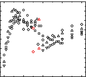
The variation in St with Re is presented in figure 21 for a number of representative L/d values in each flow regime. In the extended-body regime, St at L/d = 1.4 increases from 0.118 at Re = 2.8 × 10³ to 0.14 at Re = 1.3 × 10⁴ and then decreases slowly for further increase in Re. The initial increase in St at relatively low Re is probably connected to a reduced flow separation angle and hence a reduced wake width (Xu et al. Reference Xu, Zhang, Gan, Li and Zhou2017). Xu & Zhou (Reference Xu and Zhou2004) discussed the dependence of St on Re for two in-line circular cylinders and observed a climb in St with increasing Re for Re < 1.3 × 10³ (L/d = 1 ~ 1.5). In the wake of two tandem square cylinders, this rise in St is extended to Re ≈ 7.0 × 10³–1.03 × 10⁴. The decrease in St may be ascribed to the increased wake width with increasing Re (Bai & Alam Reference Bai and Alam2018). The decrease in St starts at the same Re for L/d = 1.2 but at Re = 5.4 × 10³ for L/d = 1.0 (figure 21a). In the reattachment regime, at L/d = 2.0, St firstly increases from Re = 2.8 × 10³ to 5.4 × 10³ before a slow drop up to Re = 2.0 × 10⁴ and then waxes and wanes from Re = 2.0 × 10⁴ to 2.8 × 10⁴ (figure 21b). The drop might be connected to the fact that the increase in Re induces a shift in the shear layer reattachment point toward the leading edge (Zhou et al. Reference Zhou, Feng, Alam and Bai2009), and the ensuing effect on St is similar to that due to an increase in L/d (figure 3). In the co-shedding regime (figure 21c), St is little sensitive to Re for Re < 5.4 × 10³ and is insensitive for Re > 5.4 × 10³. The effect of the downstream cylinder on the upstream cylinder wake decreases gradually with increasing L/d so that the variation in St with Re qualitatively approaches that in the isolated square cylinder wake.
Dependence of Strouhal number St on Re for L/d = 1.0–5.0: (a) extended-body regime, 1.0 ≤ L/d < 1.6; (b) reattachment, 1.6 ≤ L/d < 2.8–3.6; (c) co-shedding, L/d > 2.8–3.6, along with an isolated square cylinder wake.

Figure 22 presents the dependence of the flow regimes on Re and L/d, estimated based on the present measurements. The dashed line at L/d = 1.5–2.0 corresponds to the maximum St in the St–L/d relationship (figure 3), which is the turning point where the shear layer changes from direct rollup behind the cylinders to reattachment on the side surface of the downstream cylinder. The dashed line separates the extended-body and reattachment flow regimes, while the two solid lines enclose the transition regime L/d = 2.7 ~ 3.4, separating the reattachment and co-shedding regimes. The transition regime is determined based on the discontinuous drop in St (figure 3). The critical spacing (L/d)c, associated with the transition declining with increasing Re, follows the dashed line separating the extended-body and reattachment regimes. The width of the reattachment regime in terms of L/d is thus more or less constant, regardless of Re. The declining (L/d)c is ascribed to the contracted vortex formation length of a single square cylinder (Bai & Alam Reference Bai and Alam2018; Wang et al. Reference Wang, Alam and Zhou2018).
Dependence of flow regimes (extended-body, reattachment, transition and co-shedding regimes) on cylinder spacing ratio L/d and Re. The broken curve joins the points where the extended regime ends, while the two solid curves mark the starting points of the transition and co-shedding regimes, respectively.

It is of fundamental importance to compare the dependence of the flow regime on Re and L/d (figure 22) with its counterpart in the wake of two tandem circular cylinders (figure 8 in Xu & Zhou Reference Xu and Zhou2004). The difference between the square and circular cylinder wakes is, in essence, the manner in which flow separates from the cylinder, one with a fixed separation point and the other with a non-stationary oscillating separation point. Therefore, such a comparison can be insightful for the effect of flow separation on the wake dynamics. A number of interesting observations can be made from this comparison.
Firstly, the four regimes, clearly separated in the Re–L/d phase plane, are different from those in the circular cylinder wake. While Zdravkovich (Reference Zdravkovich1987) classified, based on the behaviours of the separated flow, the wake of two tandem circular cylinders into three regimes, i.e. the extended-body, reattachment and co-shedding regimes. Xu & Zhou (Reference Xu and Zhou2004) proposed four distinct categories of the St–Re relationships in the L/d–Re phase plane (Re = 8.0 × 10² ~ 4.2 × 10⁴, L/d = 1 ~ 15). Category 1 (1 ≤ L/d < 2) corresponds to the extended-body regime. Category 2 (2 ≤ L/d ≤ 3) was characterized by a transition from the extended-body regime to shear layer reattachment on the downstream cylinder. Category 3 (3 < L/d ≤ 5) was a different transition from the reattachment to the co-shedding regime. Category 4 (L/d > 5) was the co-shedding regime. Categories 2 and 3, corresponding to the reattachment regime, are each associated with one bi-stability, i.e. stable rollup beyond the downstream cylinder and stable reattachment for category 2 and stable reattachment and stable co-shedding for category 3. The latter is captured again in the present wake of two tandem square cylinders but the former is not. It seems plausible that the non-stationary oscillation of the flow separation point in the wake of circular cylinders may produce a pronounced influence on the separated shear layer so that the shear layer is also characterized by appreciable oscillation, which acts to promote the occurrence of the bi-stable phenomena in the circular cylinder wake. As such, two bi-stabilities take place. On the other hand, the shear layer separated from a fixed point is relatively stable, albeit with its intrinsic instability. The bi-stable phenomenon, stable reattachment to stable co-shedding, thus occurs only over a very narrow range of L/d (= 2.7 ~ 3.3) when the separated shear layer hits the leading corner of the downstream cylinder. The other bi-stability, stable rollup and stable reattachment, however, could not be captured presently at all although the change in the flow structure from the extended to reattachment flow is expected to be discontinuous. It seems plausible that the leading corner of the downstream cylinder plays a more important role in the fluid dynamics of this flow than its downstream counterpart.
Secondly, the St in the extended-body regime rises rapidly with increasing L/d in the wake of two tandem square cylinders (figure 3) but drops quickly in the wake of two tandem circular cylinders (figure 3 in Xu & Zhou Reference Xu and Zhou2004). The former is associated with a large flow separation angle (e.g. Xu et al. Reference Xu, Zhang, Gan, Li and Zhou2017) or initially thick shear layer. Thus, an increased L/d implies an increased after body and hence a reduced wake width, causing a rising St, as discussed in § 3. On the other hand, the flow separation angle of the latter is small and the separated shear layer is initially thin. Then an increasing L/d allows the free shear layers to grow thicker before rolling up behind the cylinders, leading to a decreased St (Xu & Zhou Reference Xu and Zhou2004).
Thirdly, (L/d)c depends appreciably on Re (figure 22). Nevertheless, this dependence is much weaker than that in the wake of two circular cylinders (figure 8, Xu & Zhou Reference Xu and Zhou2004). This is because (L/d)c is largely dependent on the vortex formation length of the upstream cylinder, which is less sensitive to Re (> 103) for the square cylinder but highly sensitive for the circular cylinder (Bai & Alam Reference Bai and Alam2018).
Finally, Liu & Chen (Reference Liu and Chen2002) observed a St–L/d hysteresis phenomenon in the wake of two tandem square cylinders at Re = 2 × 10³–1.6 × 10⁴, that is, St jumped discontinuously as L/d increased progressively but dropped discontinuously at a different (L/d)c as L/d decreased progressively. For example, at Re = 2700, when L/d was progressively increased from 1.5 to 9.0, St experienced a jump at (L/d)c = 4.2 due to the flow change from the reattachment to co-shedding regime. However, the sudden drop in St occurred at (L/d)c = 3.2, instead of 4.2, when L/d was decreased from 9.0 to 1.5 and the flow changed back from the co-shedding to reattachment regime. The hysteresis phenomenon has also been observed in the wake of two tandem circular cylinders when L/d varies from 2.0 to 2.4 or from 2.4 to 2.0 (Re = 1000) by Jester & Kallinderis (Reference Jester and Kallinderis2003), which occurs at a smaller L/d range (L/d = 2.0–2.4) than the square cylinder case (L/d = 3.2–4.2).
7. Concluding remarks
The wake of two tandem square cylinders has been systematically studied over L/d = 1.0 ~ 5.0 and Re = 2.8 × 10³ ~ 2.8 × 10⁴ based on hot-wire, pressure or force, LIF flow visualization, surface-oil-flow visualization and PIV measurements. This work leads to following conclusions.
Four distinct flow regimes have been identified based on the variation of St with L/d and the behaviours of the separated shear layers, as summarized in figure 23. The extended-body regime occurs at L/d ≤ 1.5–2.0. With increasing L/d in this regime, St rises rapidly, reaching a local maximum at L/d ≈ 1.5;  ${\bar{C}_D}$ rises on the upstream cylinder but declines on the downstream cylinder, which is linked to a drop in the cylinder gap pressure;
 ${C^{\prime}_D}$ and
 ${C^{\prime}_L}$ decrease for the upstream cylinder but go up for the downstream cylinder, which is ascribed to an increase in the effective after-body length of the two-cylinder system. In the reattachment regime (L/d = 1.5–2.0 ~ 2.7–3.2), St decreases with increasing L/d. Whilst
 ${\bar{C}_D}$ and
 ${C^{\prime}_L}$ decline on both cylinders,
 ${C^{\prime}_D}$ decreases and increases on the upstream and downstream cylinders, respectively. A shift in the reattachment point toward the cylinder leading edge for larger L/d contributes to a stronger reverse flow in the gap, thus accounting for the observations on
 ${\bar{C}_D}$,
 ${C^{\prime}_D}$ and
 ${C^{\prime}_L}$ on the two cylinders. The transition regime (L/d = 2.7 ~ 3.3) between the reattachment and co-shedding regimes is characterized by a drastic drop in St and a large jump in
 ${\bar{C}_D}$,
 ${C^{\prime}_D}$ and
 ${C^{\prime}_L}$ on both cylinders. The co-shedding regime appears at L/d > 2.7–3.3, where St rises gradually with increasing L/d and approaches that in the isolated square cylinder wake. While
 ${\bar{C}_D}$ on each cylinder varies little as L/d increases, the corresponding
 ${C^{\prime}_D}$ on the downstream cylinder declines rapidly due to the weakened impingement of the gap vortices on the downstream cylinder.
Sketches of the flow structure for each flow regime. First row: extended-body regime (L/d ≤ 1.5–2.0); second row: reattachment regime (1.5–2.0 < L/d < 2.7–3.2); third row: transition regime (2.7 ≤ L/d ≤ 3.3); fourth row: co-shedding regime (3.0–3.4 ≤ L/d ≤ 5).

The value of  ${\bar{C}_D}$ is larger on the upstream cylinder than on the downstream, irrespective of the flow regime. This is, however, reversed for
 ${C^{\prime}_D}$, which is largely contributed by a large
 ${C^{\prime}_P}$ on the rear surface of the downstream cylinder in the extended and reattachment regimes and on the front surface in the co-shedding regime. The value of
 ${C^{\prime}_L}$ is greater on the downstream cylinder than on the upstream cylinder in the extended-body and reattachment regimes but this difference is not appreciable in the co-shedding regime. The unsteady shear layers separated from the upstream cylinder overshoot or reattach on the downstream cylinder in the extended-body and reattachment regimes, causing a large fluctuating pressure on the cylinder side surface and hence a large
 ${C^{\prime}_L}$ on the downstream cylinder. In the co-shedding regime, the impingement of the upstream-cylinder-generated vortices weakens vortex shedding from the downstream cylinder, resulting in a reduced
 ${C^{\prime}_L}$ on the downstream cylinder, compared with that on the upstream cylinder. The values of
 ${\bar{C}_D}$,
 ${C^{\prime}_D}$ and
 ${C^{\prime}_L}$ on both cylinders all jump from the reattachment to co-shedding state in the transition regime.
The wake of two tandem square cylinders differs in several aspects from that of circular cylinders. Firstly, there is a marked difference when the shear layers separated from the upstream cylinder reattach on the downstream cylinder. Flow reattachment in the wake of two tandem circular cylinders is characterized by two bi-stabilities: (i) stable rollup beyond the downstream cylinder and stable reattachment, and (ii) stable reattachment and stable co-shedding. However, the flow reattachment in the wake of two tandem square cylinders is characterized by only one bi-stability, i.e. stable reattachment and stable co-shedding (transition regime), and one stable reattachment (reattachment regime). It seems plausible that the non-stationary oscillation of the separation point associated with a circular cylinder is inherited by the separated shear layer, which is responsible for the occurrence of the two bi-stabilities. On the other hand, such an ‘oscillation’ is absent in the shear layers separated from a square cylinder. As a result, the bi-stable flow phenomenon is observable only when the shear layer hits the leading corner of the downstream cylinder, splitting into two parts, one rolling up between the cylinders and the other reattaching on the side surface of the downstream cylinder, as evidenced by surface-oil-flow visualization (figure 15) and the rising St from L/d = 2.5 to 2.7 (figure 11a). With the shear layer intrinsically unstable, co-shedding would occur if the rolling up shear layer overwhelms the reattachment; alternatively, reattachment would take place if the reattached shear layer dominates. Furthermore, the bi-stable state or transition regime occurs over a very narrow range of L/d (= 2.7 ~ 3.3), compared with its circular cylinder counterpart (= 3.0 ~ 5.0). Secondly, in the extended-body regime, St rises rapidly with increasing L/d in the wake of two tandem square cylinders (figure 3) but drops quickly in the wake of circular cylinders. The difference is ascribed to their distinct flow separation angles and hence the cross-sectional geometry of the two wake generators. Finally, the critical L/d at which one flow regime is changed to another depends quite appreciably on Re in the wake of two tandem square cylinders, albeit not so much as its circular cylinder counterpart. This dependence is ascribed to the dependence on Re of the flow separation angle and the vortex formation length.
The comparison between the circular and square cylinder wakes in terms of the bi-instabilities may provide a clue on the origin of the bi-stability in the wake of a simplified automotive body, i.e. a square-back Ahmed body, as reported by Grandemange, Gohlke & Cadot (Reference Grandemange, Gohlke and Cadot2013) and other investigators (Zhou & Zhang Reference Zhou and Zhang2021). Haffner et al. (Reference Haffner, Borée, Spohn and Castelain2020) proposed that the mechanism of this bi-stability could be understood through entrainment balance considerations, which might be generalized to other geometrical configurations. Aasland et al. (Reference Aasland, Pettersen, Andersson and Jiang2023) observed long-term asymmetry of gap vortices in the two tandem circular cylinder wake, suggesting that the bi-stability mechanism they observed might be related to the long-term dynamical behaviour of the gap flow between the cylinders. The present study proposes a different mechanism, that is, a square-back Ahmed body is like a cuboid, although its two front side corners are rounded (not sharp corners), implying the occurrence of non-stationary oscillation of separation points. Such a non-stationary oscillation feature can be inherited by the separated shear layer, leading to a possible bi-stable phenomenon in the wake. The origin and mechanism of this bi-stable phenomenon, in spite of its engineering significance, has never been unveiled previously.
It is worth highlighting that the present Re range is 2.8 × (103 ~ 104). Given much higher Reynolds numbers in engineering applications, it is of practical importance to conduct further investigations at Re > 105.
Funding
Y.Z. wishes to acknowledge support given to him from NSFC through grants 91952204 and from the Research Grants Council of Shenzhen Government through grant JCYJ20210324132816040.
Declaration of interests
The authors report no conflict of interest.
Nomenclature
- C̅ D
mean drag force coefficient
- C′ D
fluctuating drag force coefficient
- C′ L
fluctuating lift force coefficient
- C̅ P
mean pressure coefficient
- C̅ Po
mean pressure coefficient of isolated cylinder
- C′ P
fluctuating pressure coefficient
- C′ Po
fluctuating pressure coefficient of isolated cylinder
- d
side length of square cylinder
- E u
power spectral density function
- f
vortex-shedding frequency
- f s
predominant vortex frequency
- f sampling
sampling frequency
- f sl
shear layer instability frequency
- FFT
fast Fourier transform
- HT1
hot-wire 1 placed in the gap between the cylinder
- HT2
hot-wire 2 placed behind the downstream cylinder
- L
distance between the cylinder centres
- L/d
centre-to-centre spacing ratio
- L f
wake formation length
- N w
FFT window size
- Re
Reynolds Number
- St
Strouhal number
- St o
Strouhal number of isolated cylinder
- T u
turbulence intensity
- u
streamwise fluctuating velocities
- u 1
streamwise fluctuating velocities measured by HT1
- u 2
streamwise fluctuating velocities measured by HT2
- u rms
root-mean-square values of streamwise velocities
- U̅
time-averaged velocity
- U c
convection velocity
- U ∞
free-stream velocity
- ν
kinematic viscosity
- w
wake width
- Δƒ
frequency resolution
- φ
phase
- ω z
spanwise vorticity
- (⋅̅)
time-averaged value
- (⋅)*
dimensionless value
- (⋅)′
fluctuating velocity component
- (⋅)rms
root-mean-square value
- (L/d)c
critical centre-to-centre spacing ratio
- (x, y, O)
coordinate with the origin at the upstream cylinder centre
- (x′, y′, O′)
coordinate with the origin at the downstream cylinder centre



