INTRODUCTION
Mangrove forests are regarded as effective sinks of atmospheric carbon because of their high net primary production (NPP) and low heterotrophic respiration (HR) (Alongi Reference ALONGI2014, Barr et al. Reference BARR, ENGEL, FUENTES, ZIEMAN, O'HALLORAN, SMITH and ANDERSON2010, Poungparn & Komiyama Reference POUNGPARN and KOMIYAMA2013). The high NPP is caused by exposure to the warm climate in the tropical zone and the lack of water restriction as soils are regularly submerged by tidal fluctuations and mangroves are tolerant to salinity (Robertson et al. Reference ROBERTSON, DANIEL and DIXON1991, Ross et al. Reference ROSS, RUIZ, TELESNICKI and MEEDER2001, Sherman et al. Reference SHERMAN, FAHEY and MARTINEZ2003). Conversely, the regular submergence leads to anaerobic conditions in the pedosphere, resulting in a low HR (Alongi et al. Reference ALONGI, WATTAYAKORN, PFITZNER, TERENDI, ZAGORSKIS, BRUNSKILL, DABIDSON and CLOUGH2001, Mall et al. Reference MALL, SINGH and GARGE1991). In mangrove forests, the CO2 flux from soil sediment to atmosphere (soil respiration) is generally regarded as HR by microbes because most below-ground metabolic respiration by plants (root respiration) is released through the lenticels on pneumatophores, prop roots and buttresses above the ground (Scholander et al. Reference SCHOLANDER, VAN DAM and SCHOLANDER1995, Tomlinson Reference TOMLINSON1986). Given these unique characteristics, previous studies assessed the HR by measuring the soil respiration rate in mangrove forests and found relatively low values (0.47–0.88 µmol CO2 m−2 s−1) compared with terrestrial tropical forests (2.21–9.94 µmol CO2 m−2 s−1) (Poungparn et al. Reference POUNGPARN, KOMIYAMA, TANAKA, SANGTIEAN, MAKNUAL, KATO, TANAPERMPOOL and PATANAPONPAIBOON2009). However, understanding of CO2 flux from the mangrove forest floor remains limited compared with the above-ground plant fixation and respiration, and therefore large uncertainties remain in estimating the ecosystem function of mangrove forests as an atmospheric carbon sink.
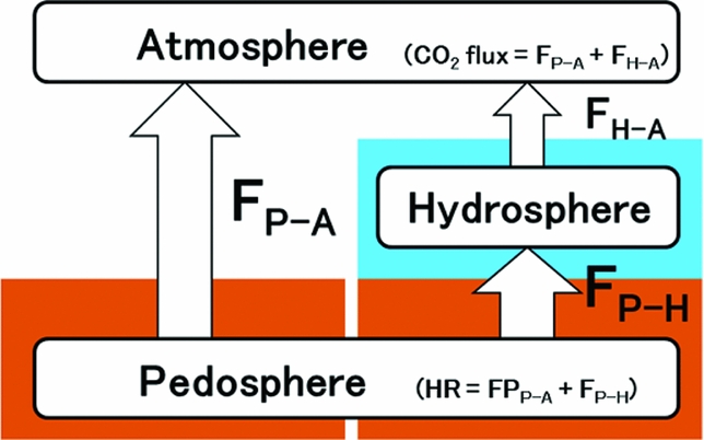
In general, soil respiration rates are largely determined by soil temperature and moisture (Davidson et al. Reference DAVIDSON, VERCHOT, CATTANIO, ACKERMAN and CARBALHO2000, Hanson et al. Reference HANSON, EDWARDS, GARTEN and ANDREWS2000). In mangrove forests, studies have reported a weak positive correlation between the soil respiration rate and soil temperature, which implies moderate seasonal variation in the soil respiration rate (Chanda et al. Reference CHANDA, AKHAND, MANNA, DUTTA, DAS, HAZRA, RAO and DADHWAL2014, Liang et al. Reference LIANG, CHANG-YI, YONG and GONG-FU2013). In contrast, the effects of soil water content on variation in mangrove soil respiration are relatively small because mangrove soils are saturated either diurnally or seasonally by tidal fluctuations, and the soil water content remains high throughout the year (Lawton et al. Reference LAWTON, TODD and NAIDOO1981). However, regular submergence of mangrove soils also affects the carbon flux by complicating the release pathway for mineralized carbon into the pedosphere. Mineralized soil carbon is emitted to the atmosphere as CO2 from the soil surface during exposed periods (FP-A, Figure 1). It is also transported to the surface water of the forest floor as dissolved inorganic carbon (DIC) flux during submerged periods (FP-H), though some DIC is emitted to the atmosphere as CO2 flux from the water surface (FH-A). Alongi et al. (Reference ALONGI, WATTAYAKORN, PFITZNER, TERENDI, ZAGORSKIS, BRUNSKILL, DABIDSON and CLOUGH2001) reported that theFP-H rate was not significantly different from the FP-A rate in many instances, and Poungparn et al. (Reference POUNGPARN, KOMIYAMA, SANGTEIAN, MAKNUAL, PATANAPONPAIBOON and SUCHEWABORIPONT2012) simply evaluated annual HR (sum of FP-A and FP-H) based on an assumption that the FP-A rate is equal to the FP-H rate. However, there have been few attempts to divide the two fluxes at the plot scale.
Emission pathways for mineralized soil carbon. FP-A indicates the flux from pedosphere to atmosphere as CO2 flux during the exposed period of soil surface. FP-H represents the flux from pedosphere to hydrosphere as dissolved flux of inorganic carbon during the submerged period. FH-A represents the flux from hydrosphere to atmosphere as CO2 flux during the submerged period.

The CO2 flux (sum of FP-A and FH-A) should directly affect the atmospheric CO2 concentration, and therefore it is especially important in understanding the role of atmospheric carbon regulation by mangrove forest. Tomotsune et al. (Reference TOMOTSUNE, SUZUKI, OHTSUKA, YOSHITAKE, SUMINOKURA, SHINKAI and KOIZUMI2017) reported that FH-A rate was 50% of FP-A rate, suggesting that the exposure/submergence regime caused by the tidal fluctuation is critical in evaluating the CO2 flux from the mangrove forest floor. However, this variable is temporally and spatially complex as tidal level changes daily, monthly and seasonally and exposure/submergence duration varies at the plot scale. Thus, the microtopography of each plot will be a key determinant, even within a single tidal cycle.
In this study, we hypothesized that the CO2 flux from the mangrove forest floor changes seasonally and is spatially dependent on the interaction between soil temperature and tidal condition. To examine this hypothesis, we measured CO2 fluxes and soil temperature in the four seasons (June, September and January 2012, and May 2013) in two study plots with different vegetation and elevation. We then estimated annual HR and CO2 flux with the consideration of soil temperature and the exposure/submergence regime.
MATERIALS AND METHODS
Study site
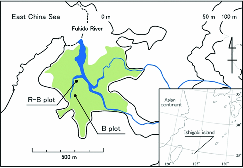
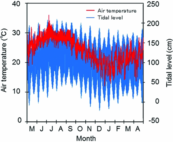
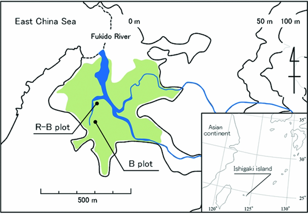
The study site is located near the Fukido River on Ishigaki Island, Okinawa Prefecture, south-western Japan (24°29ʹN, 124°13ʹE, Figure 2). The subtropical climate had an annual mean temperature of 24.3°C and mean precipitation of 2107 mm between 1981 and 2010 (Ishigakijima Local Meteorological Observatory, Japan Meteorological Agency; ILMO). Average monthly air temperature was highest in July and lowest in January, and the average tidal level was highest in August and lowest in January (Figure 3). This area is dominated by two mangrove species, Bruguiera gymnorrhiza and Rhizophora mucronata. Mangrove forests, periodically inundated by seawater, form zones of vegetation with the dominant tree species changing with distance from the seashore (Bunt Reference BUNT1996, Youssef & Saenger Reference YOUSSEF and SAENGER1999). At this site, R. mucronata is more dominant closer to the river than B. gymnorrhiza. Some respiratory mangrove roots protrude from the soil surface and there is no understorey. The pedosphere is subject to substantial deposition of mud.
Study site located near the Fukido River on Ishigaki Island, Okinawa Prefecture, south-western Japan (24°29ʹN, 124°13ʹE). Blue and green zones indicate mangrove forest and river, respectively. Permanent quadrats were established in the Bruguiera gymnorrhiza forest (B plot) and the mixed Rhizophora mucronata and B. gymnorrhiza forest (R-B plot) in May 2012.
Seasonal variation in air temperature and tidal level from May 2012 to April 2013 measured by the Ishigakijima Local Meteorological Observatory, Japan Meteorological Agency.

Permanent quadrats were established in the B. gymnorrhiza plot (B plot, 30 × 30 m) and mixed R. mucronata and B. gymnorrhiza plot (R-B plot, 20 × 30 m) in May 2012. The B plot is located farther from the estuary and has higher elevation than the R-B plot (Figure 2). Tree biomass of the B plot was 110 Mg C ha−1, whereas that of the R-B plot was 30 Mg C ha−1 (R. mucronata, 25%; B. gymnorrhiza, 75%). Average total soil carbon contents at 0–100 cm soil depth were slightly lower in the B plot (2.5%) than in the R-B plot (3.5%). The total soil organic carbon in the same sediment layer was also lower in the B plot (200 Mg C ha−1) than in the R-B plot (240 Mg C ha−1). Sand and small stones were present in the mud of the B plot.
Measurement of CO2 flux and soil temperature during the exposed period
A closed-chamber method including a portable infrared gas analyser (GMP343; VAISALA, Finland) and vinyl chloride chambers (area, 78.5 cm2; height, 11 cm) (Tomotsune et al. Reference TOMOTSUNE, MASUDA, YOSHITAKE, ANZAI and KOIZUMI2013a, Reference TOMOTSUNE, YOSHITAKE, WATANABE and KOIZUMIb) was used to measure CO2 flux during the exposed period. To clarify the seasonal variation, CO2 flux from the air-exposed soil surface (not covered with water, namely exposed period) was measured in four seasons (June, September and January 2012, and May 2013) in each forest. Measurements were conducted on 40 randomly distributed plots in each forest except for June 2012 (20 plots).
The soil temperature at 5-cm soil depth was also recorded at the time of the CO2 flux measurement by a portable thermo sensor (AD-5622, A&D, Tokyo, Japan). In addition, the soil temperature (5-cm soil depth) was continuously recorded using a temperature sensor with a data logger (UTBI-001; Onset Computer Corporation, Bourne, MA, USA) from June 2012 to March 2013. We examined the linear correlation between ILMO air temperature data (Figure 3) and site-specific soil temperature data, and then estimated continuous soil temperature for each forest from May 2012 to April 2013 (1 y).
The soil surface in the B and R-B plots was covered with water at the 147 cm and 102 cm tidal level of ILMO data, respectively. Therefore, the monthly exposure ratio at each forest was calculated based on these threshold values and continuous tidal level data supplied by the ILMO (Figure 3).
Data analysis
To clarify the relationships between CO2 flux and soil temperature, we used the following exponential equation:
 $$\begin{equation}
F = \alpha {{\mathrm{e}}^{\beta T }},
\end{equation}$$
where F is the CO2 flux (mg CO2 m−2 h−1), T is soil temperature at 5-cm depth (°C), and α and β are fitted parameters. To compare CO2 fluxes between the B and the R-B plots under the same soil temperature conditions, CO2 flux at 10°C, 20°C and 30°C (R10, R20 and R30, respectively) were calculated using Equation (1).
To clarify the effect of tidal condition on variation in the CO2 flux, the monthly and annual HR and CO2 flux was estimated based on assumptions described by Poungparn et al. (Reference POUNGPARN, KOMIYAMA, SANGTEIAN, MAKNUAL, PATANAPONPAIBOON and SUCHEWABORIPONT2012) and Tomotsune et al. (Reference TOMOTSUNE, SUZUKI, OHTSUKA, YOSHITAKE, SUMINOKURA, SHINKAI and KOIZUMI2017) and compared with each other. In Poungparn et al. (Reference POUNGPARN, KOMIYAMA, SANGTEIAN, MAKNUAL, PATANAPONPAIBOON and SUCHEWABORIPONT2012), annual HR was simply calculated based on the assumption that FP-H rate was equal to FP-A rate (Figure 1). Therefore, continuous hourly HR was calculated from Equation (1) and continuous soil temperature data during the entire period. The sum of continuous hourly HR was regarded as monthly and annual HR. In contrast, Tomotsune et al. (Reference TOMOTSUNE, SUZUKI, OHTSUKA, YOSHITAKE, SUMINOKURA, SHINKAI and KOIZUMI2017) reported that FH-A rate was 50% of FP-A rate. Then, continuous hourly CO2 flux was also estimated from Equation (1) and continuous soil temperature, but the continuous hourly CO2 flux was halved only during the submerged period. The monthly and annual CO2 flux was calculated as the sum of these values.
All statistical analysis was performed using SPSS software for Windows (SPSS Statistics 17.0, SPSS Inc., Chicago, IL, USA). Statistical comparisons were conducted using two-way analysis of variance (ANOVA) (season × forest type) and Tukey multiple comparison as the post hoc test. Significant differences for all statistical tests were evaluated at the P < 0.05 level.
RESULTS
Measured CO2 fluxes and responses to soil temperature
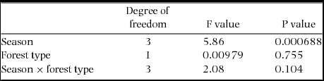
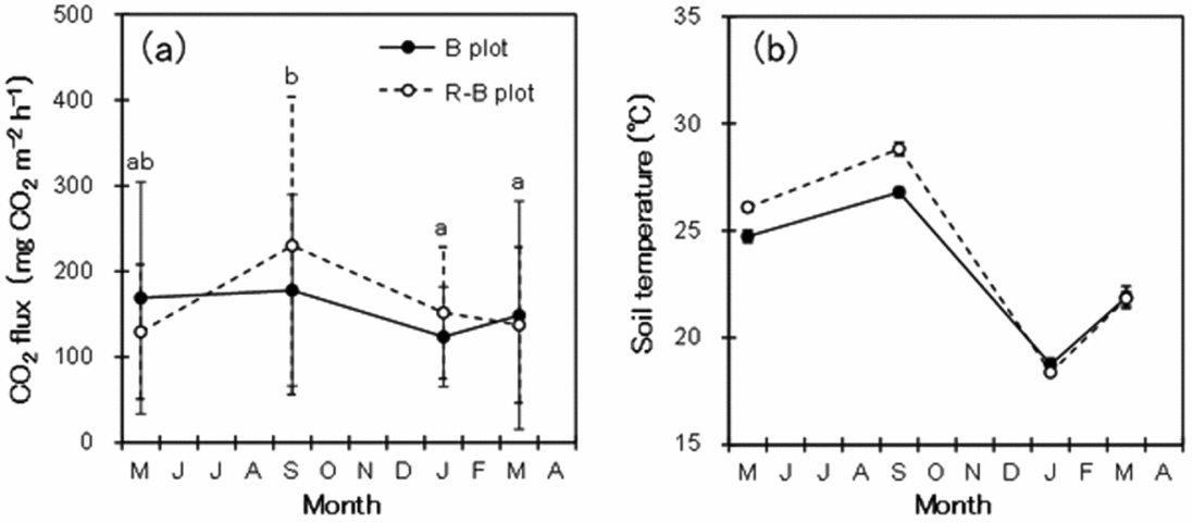
There was no significant interaction in CO2 flux between season and forest type and the main effect of forest type was not significant (two-way ANOVA; Table 1). In contrast, there was a significant main effect of season and the average CO2 flux was highest in September in both forests and lowest in January and March in the B plot and the R-B plot, respectively (Figure 4a).
Two-way analysis of variance (ANOVA) (season × forest type) for CO2 flux from the air-exposed soil surface in the Bruguiera gymnorrhiza forest (B plot) and mixed Rhizophora mucronata and B. gymnorrhiza forest (R-B plot) during four seasons (June, September and January 2012, and May 2013). Significant differences for all statistical tests were evaluated at the P < 0.05 level.

Seasonal variation in average CO2 flux from the air-exposed soil surface (a) and average soil temperature at 5 cm depth (b) in the Bruguiera gymnorrhiza forest (B plot) and mixed Rhizophora mucronata and B. gymnorrhiza forest (R-B plot), south-western Japan. The difference in CO2 flux was significant only between seasons. Different letters indicate significant differences between seasons (a). Error bars indicate standard deviation.

Average soil temperature was highest in September and lowest in January in both forests (Figure 4b). Measured soil temperature was higher in the R-B plot than in the R plot during March to September, whereas the difference was very small during January to March.
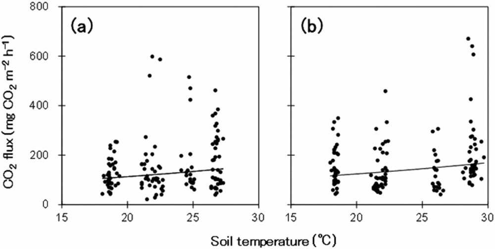
There was a weak positive correlation between CO2 flux and soil temperature in both forests (B plot: F = 51.0e0.04T, R 2 = 0.040, P < 0.05; R-B plot: F = 60.5e0.04T, R 2 = 0.07, P < 0.05) (Figure 5). Estimated R10, R20 and R30 in the B plot (77, 116 and 175 mg CO2 m−2 h−1, respectively) were slightly lower than those in the R-B plot (88, 127 and 184 mg CO2 m−2 h−1, respectively). In addition, some measured CO2 fluxes deviated substantially from the regression lines.
Relationships between CO2 flux and soil temperature at 5-cm depth in (a) Bruguiera gymnorrhiza forest and (b) mixed Rhizophora mucronata and B. gymnorrhiza forest, respectively.

Temporal variation in soil temperature and exposure duration
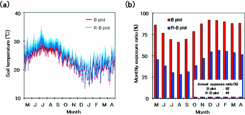
The air temperature measured by ILMO showed a strong correlation with soil temperature measured in each forest (B plot: y = 0.86x + 2.93, R 2 = 0.83, P < 0.05; R-B plot: y = 0.91x + 2.60, R 2 = 0.85, P < 0.05). Estimated soil temperature was highest in July and lowest in January and the average annual soil temperature in the B plot (23.6°C) was slightly lower than that in the R-B plot (24.4°C) (Figure 6a).
Seasonal variation in estimated soil temperature (a) and the monthly exposure ratio (b). Red and blue bars indicate the Bruguiera gymnorrhiza forest (B plot) and mixed Rhizophora mucronata and B. gymnorrhiza forest (R-B plot), respectively.

Calculated monthly exposure ratio was highest in December and lowest in August in both forests (Figure 6b) and this trend was contrary to that of soil temperature. The annual exposure ratio in the B plot (82%) was higher than that in the R-B plot (44%).
Estimated seasonal variation in HR and CO2 flux and their annual values
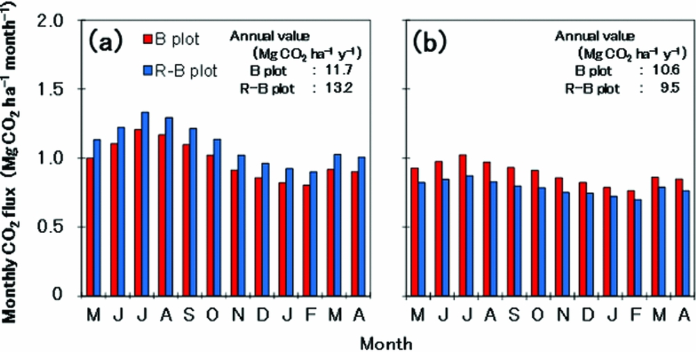
Monthly HR based on the assumption that FP-H rate is equal to FP-A rate was highest in June and lowest in February, reflecting the soil temperature (Figure 7a). The ratio of warm-season (May–October) to annual HR was 56% in both forests. The annual HR was lower in the B plot (11.7 Mg CO2 ha−1 y−1) than in the R-B plot (13.2 Mg CO2 ha−1 y−1). However, monthly CO2 flux based on the assumption that FH-A rate is 50% of FP-A rate was also highest in June and lowest in February but the seasonal difference was much smaller than that observed in the HR (Figure 7b). The ratio of warm-season to annual CO2 flux was 51% and 46% in the B and R-B plot, respectively. In addition, the annual CO2 flux was higher in the B plot (10.6 Mg CO2 ha−1 y−1) than in the R-B plot (9.5 Mg CO2 ha−1 y−1), whereas the opposite was shown for annual HR.
Calculated seasonal variation in monthly HR (a) and CO2 flux (b) in the Bruguiera gymnorrhiza forest (B plot) and mixed Rhizophora mucronata and B. gymnorrhiza forest (R-B plot). The monthly and annual HR was calculated based on the assumption in which FP-H rate is equal to FP-A rate in (a). The monthly and annual CO2 fluxes were calculated based on the assumption that FH-A rate is 50% of FP-A rate in (b). The red and blue bars indicate the flux in the B and R-B plots, respectively.

DISCUSSION
A few previous studies have measured CO2 fluxes in the exposed period in tropical mangrove forest as follows: 0.19–0.61 µmol CO2 m−2 s−1 (Alongi et al. Reference ALONGI, WATTAYAKORN, PFITZNER, TERENDI, ZAGORSKIS, BRUNSKILL, DABIDSON and CLOUGH2001), 0.05–1.47 µmol CO2 m−2 s−1 (Alongi et al. Reference ALONGI, TIRENDI and CLOUGH2000) and 0.46–0.88 µmol CO2 m−2 s−1 (Poungparn et al. Reference POUNGPARN, KOMIYAMA, SANGTEIAN, MAKNUAL, PATANAPONPAIBOON and SUCHEWABORIPONT2012). Our measured average CO2 fluxes (0.97 µmol CO2 m−2 s−1 in the B plot and 1.05 µmol CO2 m−2 s−1 in the R-B plot) were within the same range. Poungparn et al. (Reference POUNGPARN, KOMIYAMA, TANAKA, SANGTIEAN, MAKNUAL, KATO, TANAPERMPOOL and PATANAPONPAIBOON2009) reported that CO2 fluxes in the exposed period significantly differed along the zonation pattern of mangrove species, but no significant difference was observed in our study. This could be because our study site has a smaller river basin and unclear zonation of mangrove compared with the study area of Poungparn et al. (Reference POUNGPARN, KOMIYAMA, TANAKA, SANGTIEAN, MAKNUAL, KATO, TANAPERMPOOL and PATANAPONPAIBOON2009). These values reported in the mangrove forest were relatively lower than those in terrestrial tropical forests (2.13–14.1 µmol CO2 m−2 s−1; reviewed by Poungparn et al. Reference POUNGPARN, KOMIYAMA, TANAKA, SANGTIEAN, MAKNUAL, KATO, TANAPERMPOOL and PATANAPONPAIBOON2009), probably because root respiration was not included in the soil respiration of mangrove forests and HR (organic matter decomposition) would be relatively low under the anaerobic pedosphere conditions. In the present study, a high CO2 flux was occasionally observed in some plots despite the low average value. Similar phenomena were reported for a tidal flat by Sasaki et al. (Reference SASAKI, NAKAO, YOSHITAKE and NAKATSUBO2014) and were attributed to macrobenthos burrows, which increase the interface between soil and atmosphere, and consequently increase aerobic decomposition speed.
Weak positive correlations between CO2 flux and soil temperature were observed in the current study, supporting the findings of previous mangrove studies (Chanda et al. Reference CHANDA, AKHAND, MANNA, DUTTA, DAS, HAZRA, RAO and DADHWAL2014, Liang et al. Reference LIANG, CHANG-YI, YONG and GONG-FU2013). These weak correlations were caused by moderate seasonal variation in HR, with the high values occurring in the warm season. However, tidal fluctuations, which are characteristic of mangrove forests, complicate the spatiotemporal variation in CO2 flux. The tidal level is generally higher in the warm season than the cool season, and consequently the exposure duration is much shorter in the warm season. The CO2 flux during the submerged period was half that when exposed. Thus the monthly CO2 flux was relatively low during the warm season and showed a lower seasonal variation than HR. In addition, the R-B plot (lower elevation and shorter exposure duration) had a lower annual CO2 flux than the B plot (low measured CO2 flux and soil temperature). Previous studies have not focused on seasonal and microgeographic variations in exposure duration and tidal fluctuation, but have simply estimated the annual HR based on several plots (Poungparn et al. Reference POUNGPARN, KOMIYAMA, SANGTEIAN, MAKNUAL, PATANAPONPAIBOON and SUCHEWABORIPONT2012). However, our results suggest that the spatiotemporal variation in exposure duration is an important factor in evaluating the annual CO2 flux at a local scale and understanding the role of atmospheric CO2 regulation in mangrove forests.
The difference of HR and CO2 flux in this study indicated the dissolved flux was DIC, which was calculated as 1.1 and 3.6 Mg CO2 ha−1 y−1 in the B and R-B plot, respectively. However, current understanding of the DIC flux is insufficient and the mechanism of carbon loss as DIC flux has not yet been adequately clarified (Maher et al. Reference MAHER, SANTOS, GOLSBY-SMITH, GLESSON and EYRE2013). Breithaupt et al. (Reference BREITHAUPT, SMOAK, SMITH, SANDERS and HOARE2012) argued that the products (organic carbon) in mangrove forests would flow out at 45% for uncounted carbon including DIC export. To understand the contribution of gaseous and dissolved fluxes to the HR, future research should more precisely clarify the transport process of carbon flux from soil sediments to overlying water and from water to the atmosphere during submergence and the spatiotemporal variation of exposure duration at the local scale.
Our study clarified that CO2 flux showed moderate seasonality, reflecting the interaction between the seasonal trend in soil temperature and the contrary trend in exposure duration. In addition, seasonal and microgeographic variation in exposure duration on the forest floor directly affect the evaluation of CO2 flux in mangrove ecosystems. These findings contribute to our understanding of the dynamics of the carbon stock in the mangrove pedosphere and the role of mangroves as a regulator of atmospheric CO2.
ACKNOWLEDGEMENTS
We thank Dr Kinjo, University of the Ryukyus for help with the field research and useful advice. We also thank the laboratory members of Gifu University, Kobe University and Waseda University for their assistance in field measurements and many constructive discussions. This work was supported by the Sasakawa Scientific Research Grant from The Japan Science Society. We thank Edanz Group (www.edanzediting.com/ac) for editing a draft of this manuscript.