1 Introduction
Size segregation of polydisperse granular materials is ubiquitous in industrial and natural processes. As particles of different sizes flow or are agitated in the presence of gravity, small particles fall through the interstices between larger particles resulting in size segregation of initially well-mixed particles. This mechanism is commonly referred to as particle percolation; it is the primary driving mechanism for segregation in dense size-disperse granular flow and its effects are the focus of this paper.
Most previous theoretical approaches to understanding and modelling percolation-driven segregation have been limited to bidisperse granular mixtures (Savage & Lun Reference Savage and Lun1988; Dolgunin, Kudy & Ukolov Reference Dolgunin, Kudy and Ukolov1998; Gray & Thornton Reference Gray and Thornton2005; Gray & Chugunov Reference Gray and Chugunov2006; May et al. Reference May, Golick, Phillips, Shearer and Daniels2010; Fan & Hill Reference Fan and Hill2011; Wiederseiner et al. Reference Wiederseiner, Andreini, Epely-Chauvin, Moser, Monnereau, Gray and Ancey2011; Marks, Rognon & Einav Reference Marks, Rognon and Einav2012; Thornton et al. Reference Thornton, Weinhart, Luding and Bokhove2012; Larcher & Jenkins Reference Larcher and Jenkins2013, Reference Larcher and Jenkins2015; Tunuguntla, Bokhove & Thornton Reference Tunuguntla, Bokhove and Thornton2014). Several studies have used experiments (Newey et al. Reference Newey, Ozik, Van der Meer, Ott and Losert2004; Conway et al. Reference Conway, Lekhal, Khinast and Glasser2005; Jain, Metzger & Glasser Reference Jain, Metzger and Glasser2013; Bhattacharya & McCarthy Reference Bhattacharya and McCarthy2014) and discrete element method (DEM) simulations (Marks et al. Reference Marks, Rognon and Einav2012; Jain et al. Reference Jain, Metzger and Glasser2013; Pereira & Cleary Reference Pereira and Cleary2013; Bhattacharya & McCarthy Reference Bhattacharya and McCarthy2014) to study polydisperse segregation, but a general theoretical model for polydisperse segregation is currently lacking. Gray & Ancey (Reference Gray and Ancey2011) derived a continuum equation that describes the segregation of multidisperse mixtures (i.e. a finite number of distinct particle sizes), but the model includes arbitrarily adjustable parameters, making it difficult to accurately apply the results to specific particle sizes or to generalize the model to a continuous distribution of particle sizes. Marks et al. (Reference Marks, Rognon and Einav2012) developed a continuum model for polydisperse segregation, but it also relies on a fitting parameter without a clear physical meaning that is determined by fitting data to DEM simulations in an ad hoc manner, making it difficult to apply the model across a broad range of physical parameters. Recently a stochastic lattice model incorporating the effects of segregation, mixing and crushing was applied to predict steady-state grain size distributions in uniformly sheared granular flows (Marks & Einav Reference Marks and Einav2015). Although the approach can connect micro and macroscale advection-driven processes for polydisperse systems, it has shown only qualitative agreement with experimental grain size distributions in geophysical situations such as debris flows and fault gouges. Moreover, only a limited number of initial size distribution types have been considered, such as uniform or power-law distributions, even though in typical granular systems in industry and nature, particle sizes tend to be distributed log normally (Peng & Dai Reference Peng and Dai1994; Limpert, Stahel & Abbt Reference Limpert, Stahel and Abbt2001; Su & Yu Reference Su and Yu2005; Bartelt & McArdell Reference Bartelt and McArdell2009; Bertin et al. Reference Bertin, Cotabarren, Bucula and Pina2011).
In this paper, we generalize a recent segregation model for bidisperse gravity-driven flows (Fan et al. Reference Fan, Schlick, Umbanhowar, Ottino and Lueptow2014) to describe segregation in multidisperse mixtures by extending the bidisperse percolation velocity model to describe interactions between particles of three or more different sizes. Our model is similar to the approach of Gray & Ancey (Reference Gray and Ancey2011); however, it utilizes physical segregation parameters and material dependent scalings obtained from DEM simulations that are applicable to different flows. Using this formalism, we generalize the model to describe segregation in polydisperse mixtures of particles. We apply the model to two different examples of gravity-driven flows: tridisperse heap flow and polydisperse chute flow, though the model is broadly applicable to many types of granular flows. In these examples, the theoretical model demonstrates quantitative agreement with DEM simulations. In the polydisperse chute flow example, the model is applied first to particle sizes that are distributed log normally by volume, though other particle size distributions are also considered.
The relevance of polydisperse particle segregation in heap and chute flow to industrial settings is clear: segregation is problematic in industries ranging from pharmaceutical production to polymer processing to handling of ores and grains. The model may also be applicable to geophysical settings, such as debris flow, although this is a complex area where specific details are of critical importance (Montgomery & Buffington Reference Montgomery and Buffington1997) and where even defining consistent terminology presents challenges (Mulder & Alexander Reference Mulder and Alexander2001). It has been argued that simple physical models of granular solids and solid–fluid mixtures may provide a foundation for the development of a comprehensive theory of debris flow (Iverson Reference Iverson1997), and various groups have attempted to model particle segregation as a combination of sediment particles of various sizes and a fluid flowing down a chute (Hutter, Svendsen & Rickenmann Reference Hutter, Svendsen and Rickenmann1996). Here we provide the foundation for theoretically modelling percolation-driven segregation in multidisperse and polydisperse granular flows with the ultimate goal of providing a robust theoretical approach for segregating granular materials in both industrial and geophysical situations.
2 Multidisperse mixtures
In the bidisperse segregation model of Fan et al. (Reference Fan, Schlick, Umbanhowar, Ottino and Lueptow2014), the effects of segregation are combined with advection due to the mean flow and diffusion due to random particle collisions through a scalar transport equation:
 $$\begin{eqnarray}\frac{\partial c_{i}}{\partial t}+\boldsymbol{{\rm\nabla}}\boldsymbol{\cdot }(\boldsymbol{u}c_{i})+\frac{\partial }{\partial z}(w_{p,i}c_{i})=\boldsymbol{{\rm\nabla}}\boldsymbol{\cdot }(D\boldsymbol{{\rm\nabla}}c_{i}),\end{eqnarray}$$
where
 $\boldsymbol{u}=u\hat{\boldsymbol{x}}+v\hat{\boldsymbol{y}}+w\hat{\boldsymbol{z}}$
is the mean particle velocity with streamwise, spanwise and normal components,
 $u$
,
 $v$
and
 $w$
, respectively. Here,
 $x$
is the streamwise coordinate,
 $y$
is the spanwise coordinate,
 $z$
is the coordinate normal to the free surface where segregation occurs and the origin is at the free surface.
 $c_{i}$
is the volume concentration of species
 $i$
,
 $D$
is the scalar diffusion coefficient assuming that diffusion is homogeneous and isotropic and
 $w_{p,i}=w_{i}-w$
is the percolation velocity of species
 $i$
related to segregation, which accounts for the motion of different sized particles relative to the mean flow in the direction normal to the free surface. This model has been applied to bidisperse segregation in bounded heaps (Fan et al.
Reference Fan, Schlick, Umbanhowar, Ottino and Lueptow2014; Schlick et al.
Reference Schlick, Fan, Isner, Umbanhowar, Ottino and Lueptow2015a
) and rotating tumblers (Schlick et al.
Reference Schlick, Fan, Umbanhowar, Ottino and Lueptow2015b
), and its predictions exhibit excellent quantitative agreement with both DEM simulations and experiments.
The key to this model is a relation for the percolation velocity applicable to size bidisperse mixtures (Savage & Lun Reference Savage and Lun1988; Gray & Thornton Reference Gray and Thornton2005; Fan et al.
Reference Fan, Schlick, Umbanhowar, Ottino and Lueptow2014) composed of particles with diameters
 ${\it\alpha}_{i}$
and
 ${\it\alpha}_{j}$
in which the percolation velocity
 $w_{p,i}$
for species
 $i$
is related to the local shear rate
 $\dot{{\it\gamma}}$
and the local concentration of the other species (
 $j$
) as
 $$\begin{eqnarray}w_{p,i}=S({\it\alpha}_{i},{\it\alpha}_{j})\dot{{\it\gamma}}c_{j}.\end{eqnarray}$$
Here
 $S$
, the percolation length scale, is approximated as
 $$\begin{eqnarray}S({\it\alpha}_{i},{\it\alpha}_{j})=B\min ({\it\alpha}_{i},{\it\alpha}_{j})\ln ({\it\alpha}_{i}/{\it\alpha}_{j})\end{eqnarray}$$
for cohesionless spherical glass particles, where
 $B=0.26$
and the expression is valid for
 $1/3<{\it\alpha}_{i}/{\it\alpha}_{j}<3$
(Schlick et al.
Reference Schlick, Fan, Isner, Umbanhowar, Ottino and Lueptow2015a
). This expression captures the downward percolation of smaller particles (
 ${\it\alpha}_{i}<{\it\alpha}_{j}$
) and the upward segregation of larger particles (
 ${\it\alpha}_{i}>{\it\alpha}_{j}$
) in a flowing mixture. It describes the local effects of percolation, and is thus valid everywhere in a dense, bidisperse granular system.
To generalize the model to multidisperse mixtures, we assume as a first-order approximation that the percolation velocity of particle
 $i$
is a linear combination of the concentration of each surrounding species
 $j$
weighted by the percolation length scale
 $S({\it\alpha}_{i},{\it\alpha}_{j})$
and the local shear rate
 $\dot{{\it\gamma}}$
. For
 $n$
distinct particle sizes in a mixture, each with diameter
 ${\it\alpha}_{j}$
and a spatially varying concentration
 $c_{j}(\boldsymbol{x})$
where
 $j=1,\ldots ,n$
, equation (2.2) for the percolation velocity of particle
 $i$
is generalized to
 $$\begin{eqnarray}w_{p,i}=\mathop{\sum }_{j=1}^{n}S({\it\alpha}_{i},{\it\alpha}_{j})\dot{{\it\gamma}}c_{j}.\end{eqnarray}$$
Equation (2.4) is similar to the approach proposed in Gray & Ancey (Reference Gray and Ancey2011) based on the linear sum of binary interactions but with the additional inclusion of the local shear rate, consistent with (2.2), which has been successfully applied to bidisperse mixtures (Fan et al.
Reference Fan, Schlick, Umbanhowar, Ottino and Lueptow2014; Schlick et al.
Reference Schlick, Fan, Isner, Umbanhowar, Ottino and Lueptow2015a
,Reference Schlick, Fan, Umbanhowar, Ottino and Lueptow
b
). This relation neglects higher-order interactions between species, but it provides an appropriate starting point to consider multidisperse mixtures. Substituting (2.4) into (2.1) yields the full scalar transport equation for particle mixtures with
 $n$
distinct sizes:
 $$\begin{eqnarray}\frac{\partial c_{i}}{\partial t}+\boldsymbol{u}\boldsymbol{\cdot }\boldsymbol{{\rm\nabla}}c_{i}+\mathop{\sum }_{j=1}^{n}\left[S({\it\alpha}_{i},{\it\alpha}_{j})\frac{\partial }{\partial z}\left(\dot{{\it\gamma}}c_{j}c_{i}\right)\right]=\boldsymbol{{\rm\nabla}}\boldsymbol{\cdot }(D\boldsymbol{{\rm\nabla}}c_{i}).\end{eqnarray}$$
This system of
 $n$
coupled nonlinear partial differential equations can be simplified to
 $n-1$
partial differential equations since the total species concentration
 $\sum _{i=1}^{n}c_{i}=1$
.
Unlike previous approaches, equation (2.5) contains no arbitrarily adjustable fitting parameters; instead, it uses an empirical form for
 $S$
(2.3) that has been measured from DEM simulations and successfully applied to different flow geometries (Schlick et al.
Reference Schlick, Fan, Isner, Umbanhowar, Ottino and Lueptow2015a
,Reference Schlick, Fan, Umbanhowar, Ottino and Lueptow
b
). Previous studies showed that the diffusion coefficient
 $D$
depends on the local shear rate and particle size in the flowing layer (Utter & Behringer Reference Utter and Behringer2004; Fan et al.
Reference Fan, Schlick, Umbanhowar, Ottino and Lueptow2014) and saturates in the creep flow region (Fan et al.
Reference Fan, Umbanhowar, Ottino and Lueptow2015), so
 $D$
can be estimated from the flow kinematics. Therefore, (2.5) can be applied to any flowing mixture of
 $n$
discrete particle sizes when the kinematics are known. Note that in bounded heap flow we have shown that using the mean diffusion coefficient in the entire flowing layer instead of a spatially varying diffusion term provides accurate model predictions and reduces mathematical complexity significantly, so here we use the mean diffusion coefficient in the flowing layer.
To test the validity of (2.5), we consider tridisperse (
 $n=3$
) segregation in the flowing layer of quasi-two-dimensional (2-D) bounded heap flow, the same flow geometry considered in previous studies of segregation in bidisperse mixtures (Fan et al.
Reference Fan, Schlick, Umbanhowar, Ottino and Lueptow2014; Schlick et al.
Reference Schlick, Fan, Isner, Umbanhowar, Ottino and Lueptow2015a
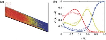
). A DEM simulation for a tridisperse mixture of spherical glass particles in a quasi-2-D bounded heap flow is used to compare predictions of the model (see figure 1
a). In quasi-2-D bounded heap flow, granular material is fed by gravity at the end of the thin gap between two coplanar vertical walls. If the material flows continuously (no avalanching), then the heap rises with uniform velocity. A linear spring-dashpot normal force and a linear spring tangential force with Coulomb sliding friction criterion were used for the contact model in the DEM simulation. A restitution coefficient
 $e=0.8$
and binary collision time
 $t_{c}=1\times 10^{-3}$
s were used to simulate contacts between glass spheres. The Coulomb sliding friction coefficient for particle–particle and particle–wall contacts was
 ${\it\mu}_{pp}={\it\mu}_{pw}=0.4$
. Further details on the methodology of the DEM simulation and quasi-2-D bounded heaps can be found in our previous work (Fan et al.
Reference Fan, Boukerkour, Blanc, Umbanhowar, Ottino and Lueptow2012, Reference Fan, Umbanhowar, Ottino and Lueptow2013, Reference Fan, Schlick, Umbanhowar, Ottino and Lueptow2014).
Tridisperse segregation in quasi-2-D bounded heap flow. (a) DEM simulation of 1 mm (dark grey, red online), 2 mm (light grey, yellow online) and 3 mm (black, blue online) diameter particles in a
 $W=46.7$
cm wide and
 $T=15$
mm thick container with feed rate
 ${\dot{m}}=11.7~\text{g}~\text{s}^{-1}$
. (b) Concentration versus scaled streamwise position at the bottom of the flowing layer for the model (curves) and the DEM simulation shown in (a) (data points) for 1 mm (dark grey, red online, ○), 2 mm (light grey, yellow online, ▫), and 3 mm (black, blue online, ▵) diameter particles.

For the tridisperse mixture in bounded heap flow shown in figure 1(a), particles enter the flowing layer well mixed, and their concentrations are approximately equal at the flow inlet (
 $c_{s}=c_{m}=c_{l}=1/3$
). The smallest particles quickly percolate to the bottom of the flowing layer and deposit in the upstream region of the heap. Intermediate size particles rise above the small particles in the flowing layer but fall below the large particles, and deposit midway down the heap. The largest particles rise to the top of the flowing layer and are advected down the heap depositing in the downstream portion of the heap.
To predict the segregation pattern for the flow shown in figure 1, equation (2.5) is solved using a mapping method with operator splitting (Fan et al.
Reference Fan, Schlick, Umbanhowar, Ottino and Lueptow2014). Particle motion occurs almost entirely in a thin flowing layer extending from the free surface to a depth of
 $O(10)$
particle diameters, and this is where we apply the theoretical model (2.5). To implement the model for tridisperse mixtures, the depth of the flowing layer
 ${\it\delta}=1.0~\text{cm}$
(assumed constant) and the diffusion coefficient
 $D=1.4\times 10^{-6}~\text{m}^{2}~\text{s}^{-1}$
are taken from previous studies (Schlick et al.
Reference Schlick, Fan, Isner, Umbanhowar, Ottino and Lueptow2015a
). The surface velocity is assumed to decrease linearly along the length of the flowing layer and the streamwise velocity is assumed to decrease exponentially with depth, consistent with mass conservation for a steadily rising surface, and validated by DEM simulations and experiments (Fan et al.
Reference Fan, Umbanhowar, Ottino and Lueptow2013).
Figure 1(b) compares the particle concentration at the bottom of the flowing layer for each of the three species for the model and the DEM simulation shown in (a). For all three species, the model agrees well with the DEM simulation. More importantly, the theoretical curves were calculated without the use of any fitting parameters; all parameter values needed for the model were determined in previous studies based on bidisperse mixtures of particles (Fan et al. Reference Fan, Schlick, Umbanhowar, Ottino and Lueptow2014; Schlick et al. Reference Schlick, Fan, Isner, Umbanhowar, Ottino and Lueptow2015a ), demonstrating the potential of this theoretical approach. We expect this approach to work for any inlet concentration of particles (not just equal concentrations) as well as for more than three species.
3 Polydisperse mixtures
Consider now a continuous distribution of particle sizes with diameters
 ${\it\alpha}_{min}<{\it\alpha}<{\it\alpha}_{max}$
. Define
 $c(\boldsymbol{x},t,{\it\alpha})\,\text{d}{\it\alpha}$
as the probability that particles with sizes between
 ${\it\alpha}$
and
 ${\it\alpha}+\text{d}{\it\alpha}$
are at position
 $\boldsymbol{x}$
at time
 $t$
. Note that
 ${\it\alpha}$
has units of length and
 $c(\boldsymbol{x},t,{\it\alpha})$
is a probability density function with units of 1/length. Generalizing (2.5) from multidisperse to polydisperse mixtures yields
 $$\begin{eqnarray}\displaystyle & & \displaystyle \frac{\partial c(\boldsymbol{x},t,{\it\alpha})}{\partial t}+\boldsymbol{u}(\boldsymbol{x},t)\boldsymbol{\cdot }\boldsymbol{{\rm\nabla}}c(\boldsymbol{x},t,{\it\alpha})+\displaystyle \int _{{\it\alpha}_{min}}^{{\it\alpha}_{max}}S({\it\alpha},{\it\alpha}^{\prime })\frac{\partial }{\partial z}[\dot{{\it\gamma}}c(\boldsymbol{x},t,{\it\alpha})c(\boldsymbol{x},t,{\it\alpha}^{\prime })]\,\text{d}{\it\alpha}^{\prime }\nonumber\\ \displaystyle & & \displaystyle \quad =\boldsymbol{{\rm\nabla}}\boldsymbol{\cdot }[D\boldsymbol{{\rm\nabla}}c(\boldsymbol{x},t,{\it\alpha})].\end{eqnarray}$$
The connection between (2.5) and (3.1) is evident by noting that for the multidisperse case with a finite number of distinct particle sizes with diameter
 ${\it\alpha}_{i}$
and concentration
 $c_{i}$
(
 $i=1,\ldots ,n$
),
 $$\begin{eqnarray}c(\boldsymbol{x},t,{\it\alpha})=\mathop{\sum }_{i=1}^{n}c_{i}(\boldsymbol{x},t){\it\delta}({\it\alpha}-{\it\alpha}_{i}),\end{eqnarray}$$
where
 ${\it\delta}({\it\alpha})$
is the Dirac delta function. Substituting this expression into (3.1) yields (2.5).
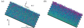
Images from a DEM simulation of chute flow for a size polydisperse granular mixture for the (a) initial condition and (b) a fully developed, segregated state after 60 s. Initially well-mixed particles flow down the chute (left to right).
 $x$
is the streamwise coordinate,
 $y$
is the spanwise coordinate,
 $z$
is the coordinate normal to the free surface, the origin is at the free surface and
 $\boldsymbol{g}$
indicates the direction of gravity. Periodic boundary conditions are implemented in the streamwise (
 $x$
) direction. Particle sizes are distributed according to a truncated log-normal distribution, with mean particle diameter
 $\bar{{\it\alpha}}\approx 2$
mm and minimum and maximum particle diameters equal to 1 mm and 4 mm, respectively. Chute inclination angle is
 ${\it\theta}=28^{\circ }$
and particle depth is
 ${\it\delta}=6.2$
cm.

3.1 Polydisperse segregation in steady-state chute flow
To demonstrate the application of the model (3.1) to polydisperse segregation, we consider chute flow in the limit of an infinitely long chute, in which the segregation of a polydisperse mixture is assumed to have reached steady state. Although the method can be applied to other dense gravity-driven flows, chute flow has the advantage of being a relatively simple flow in steady state, and it has applications to both industrial processes and geophysical debris flows (Hutter et al.
Reference Hutter, Svendsen and Rickenmann1996). A DEM simulation for polydisperse segregation in chute flow is shown in figure 2. In the simulation, particle sizes are modelled using a truncated log-normal distribution by volume with mean particle diameter
 ${\it\alpha}=2$
mm and minimum and maximum particle diameters of 1 mm and 4 mm, respectively. In an idealized chute flow, particles flow continuously down an infinitely long incline with a constant particle depth
 ${\it\delta}$
and
 $z=0$
located at the free surface. In the DEM simulation, periodic boundary conditions were implemented in the streamwise (
 $x$
) direction to simulate a fully developed, steady-state condition and to minimize the computational domain. Frictional sidewalls constrained the simulation domain in the spanwise (
 $y$
) direction, with a gap thickness
 $T=1.76$
cm and a particle–wall Coulomb sliding friction coefficient
 ${\it\mu}_{pw}=0.1$
. The bottom boundary consisted of a stationary, regular packing of small particles with diameters uniformly distributed between 1.0 and 1.5 mm, simulating a rough wall composed of glued spheres. These boundary conditions produce a steady-state velocity profile that is approximately linear through the depth of the flowing layer.
Previous DEM simulations (Silbert et al.
Reference Silbert, Ertas, Grest, Halsey, Levine and Plimpton2001; Rognon et al.
Reference Rognon, Roux, Naaim and Chevoir2007) and theory (Rognon et al.
Reference Rognon, Roux, Naaim and Chevoir2007) have approximated the velocity profile for chute flows using a Bagnold-type rheology, giving rise to a profile of the form:
 $\boldsymbol{u}\sim [{\it\delta}^{3/2}-(-z)^{3/2}]\hat{\boldsymbol{x}}$
. More complex profiles have been suggested by others to account for discrepancies in experimentally observed profile shapes across a wide variety of flowing regimes (Ancey Reference Ancey2001). Adding to this complexity are the coupled effects of size segregation on the velocity profile in non-monodisperse mixtures, which at present has received little investigation except for recent work by Marks et al. (Reference Marks, Rognon and Einav2012). However, in most studies of monodisperse flows down rough inclines, the velocity is well approximated by a linear profile for sufficiently shallow flow depths (
 ${<}$
20 particle diameters thick) (Silbert et al.
Reference Silbert, Ertas, Grest, Halsey, Levine and Plimpton2001; Midi Reference Midi2004). Consistent with the DEM results, we use a linear velocity profile in the model:
 $\boldsymbol{u}=\dot{{\it\gamma}}\left(z+{\it\delta}\right)\hat{\boldsymbol{x}}$
, where
 $\dot{{\it\gamma}}\equiv \partial u/\partial z$
is the (constant) shear rate and
 ${\it\delta}$
is the particle depth. We note that steady-state concentration distributions for a linear velocity profile (presented later in this section) were very similar to those for a Bagnold velocity profile.
For steady-state chute flow,
 $c(\boldsymbol{x},t,{\it\alpha})=c(z,{\it\alpha})$
, since the particle concentrations are independent of the streamwise position
 $x$
. Therefore, equation (3.1) becomes
 $$\begin{eqnarray}\int _{{\it\alpha}_{min}}^{{\it\alpha}_{max}}S({\it\alpha},{\it\alpha}^{\prime })\frac{\partial }{\partial z}[\dot{{\it\gamma}}c(z,{\it\alpha})c(z,{\it\alpha}^{\prime })]\,\text{d}{\it\alpha}^{\prime }=\frac{\partial }{\partial z}\left[D\frac{\partial c(z,{\it\alpha})}{\partial z}\right]\end{eqnarray}$$
for
 $-{\it\delta}\leqslant z\leqslant 0$
. The boundary conditions for (3.1) are the segregation flux equals the diffusion flux at the boundaries (
 $z=-{\it\delta},0$
). In addition, the overall particle size distribution,
 $f({\it\alpha})$
, is specified such that
 $$\begin{eqnarray}\int _{-{\it\delta}}^{0}c(z,{\it\alpha})u(z)\,\text{d}z=f({\it\alpha})\int _{-{\it\delta}}^{0}u(z)\,\text{d}z,\end{eqnarray}$$
where
 $\int _{{\it\alpha}_{min}}^{{\it\alpha}_{max}}f({\it\alpha})\,\text{d}{\it\alpha}=1$
. Note that the particle concentrations are weighted by the velocity, so that the total flux of particles through
 $-{\it\delta}\leqslant z\leqslant 0$
is specified. Integrating (3.3) with respect to
 $z$
and applying the no flux boundary condition yields
 $$\begin{eqnarray}\int _{{\it\alpha}_{min}}^{{\it\alpha}_{max}}S({\it\alpha},{\it\alpha}^{\prime })\dot{{\it\gamma}}c(z,{\it\alpha})c(z,{\it\alpha}^{\prime })\,\text{d}{\it\alpha}^{\prime }=D\frac{\partial c(z,{\it\alpha})}{\partial z}\end{eqnarray}$$
for
 $-{\it\delta}\leqslant z\leqslant 0$
. Note that the governing (3.5) specifies that, in steady state, the segregation flux equals the diffusion flux in the entire domain (
 $-{\it\delta}\leqslant z\leqslant 0$
), which is the same as the boundary condition at
 $z=-{\it\delta},0$
. This makes sense physically since, in steady state, particles do not on average move in the
 $z$
direction.
To non-dimensionalize (3.5), let
 $\tilde{z}=z/{\it\delta}$
,
 $\tilde{{\it\alpha}}={\it\alpha}/d_{0}$
,
 $\tilde{c}=d_{0}c$
,
 $\tilde{S}=S/d_{0}$
and
 $\tilde{f}=d_{0}f$
, where
 $d_{0}$
is a characteristic length associated with the particle size. Substituting these dimensionless quantities in (3.5) yields
 $$\begin{eqnarray}{\it\Gamma}\int _{\tilde{{\it\alpha}}_{min}}^{\tilde{{\it\alpha}}_{max}}\tilde{S}(\tilde{{\it\alpha}},\tilde{{\it\alpha}}^{\prime })\tilde{c}(\tilde{z},\tilde{{\it\alpha}})\tilde{c}(\tilde{z},\tilde{{\it\alpha}}^{\prime })\,\text{d}\tilde{{\it\alpha}}^{\prime }=\frac{\partial \tilde{c}(\tilde{z},\tilde{{\it\alpha}})}{\partial \tilde{z}}\end{eqnarray}$$
for
 $-1\leqslant \tilde{z}\leqslant 0$
, where
 ${\it\Gamma}=d_{0}\dot{{\it\gamma}}{\it\delta}/D$
. Using the same dimensionless quantities as above and the linear velocity profile, equation (3.4) becomes
 $$\begin{eqnarray}\int _{-1}^{0}\tilde{c}(\tilde{z},\tilde{{\it\alpha}})(1+\tilde{z})\,\text{d}\tilde{z}=\frac{1}{2}\tilde{f}(\tilde{{\it\alpha}}),\end{eqnarray}$$
with
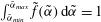 $\int _{\tilde{{\it\alpha}}_{min}}^{\tilde{{\it\alpha}}_{max}}\tilde{f}(\tilde{{\it\alpha}})\,\text{d}\tilde{{\it\alpha}}=1$
.
Equation (3.6) is similar to the steady-state advection–segregation–diffusion equation presented in Schlick et al. (Reference Schlick, Fan, Umbanhowar, Ottino and Lueptow2015b
) in that the product
 ${\it\Gamma}\tilde{S}=\dot{{\it\gamma}}{\it\delta}S/D$
represents the relative importance of segregation compared to diffusion. For bidisperse segregation in a bounded heap or rotating tumbler (Fan et al.
Reference Fan, Schlick, Umbanhowar, Ottino and Lueptow2014; Schlick et al.
Reference Schlick, Fan, Umbanhowar, Ottino and Lueptow2015b
), this ratio can be expressed as the product of a dimensionless segregation parameter,
 ${\it\Lambda}$
, representing the ratio of segregation to advection, and the Péclet number,
 $Pe$
, representing the ratio of advection to diffusion, such that
 ${\it\Lambda}Pe=\dot{{\it\gamma}}{\it\delta}S/D$
. Of course, there is no streamwise advective time scale in fully developed chute flow. Thus, the product
 ${\it\Lambda}Pe$
is analogous to
 ${\it\Gamma}\tilde{S}$
in that it represents the relative importance of segregation compared to diffusion. However, the model for polydisperse segregation differs from previous results for bidisperse systems (Fan et al.
Reference Fan, Schlick, Umbanhowar, Ottino and Lueptow2014; Schlick et al.
Reference Schlick, Fan, Isner, Umbanhowar, Ottino and Lueptow2015a
,Reference Schlick, Fan, Umbanhowar, Ottino and Lueptow
b
) in that the non-dimensional percolation length scale
 $\tilde{S}$
is not a constant. Hence, (3.6) represents a natural non-dimensionalization, where
 $\tilde{S}$
remains inside the integral, as it must. Equation (3.6) can be solved for
 $\tilde{c}(\tilde{z},\tilde{{\it\alpha}})$
using a finite difference method with the midpoint rule to approximate the integral, one-sided differencing in the
 $\tilde{z}$
direction, and the method of successive iterations (Ames Reference Ames1977) to account for the nonlinearity. For the remainder of this work, tildes are dropped and dimensional quantities are denoted with a subscript ‘
 $d$
’.
While (3.6) can be applied to any particle size distribution, here we primarily consider log-normal distributions, which are prevalent in many different scientific areas (Limpert et al. Reference Limpert, Stahel and Abbt2001). In granular systems, particle sizes have been shown to be log-normally distributed in iron–copper alloys fabricated using a coevaporation technique (Peng & Dai Reference Peng and Dai1994), aggregates of snow and ice from snow avalanches (Bartelt & McArdell Reference Bartelt and McArdell2009), urea from an industrial fluidized bed granulator (Bertin et al. Reference Bertin, Cotabarren, Bucula and Pina2011) and aerobic granules cultivated in a sequencing batch reactor (Su & Yu Reference Su and Yu2005).
The variable
 ${\it\alpha}_{d}$
is log-normally distributed with median
 $d_{0}$
and geometric standard deviation
 ${\it\sigma}_{g}$
when
 $\ln ({\it\alpha}_{d}/d_{0})$
is normally distributed with mean 0 and standard deviation
 ${\it\sigma}=\ln {\it\sigma}_{g}$
. Therefore,
 $$\begin{eqnarray}f({\it\alpha})=\frac{1}{{\it\alpha}{\it\sigma}\sqrt{2{\rm\pi}}}\exp \left[-\frac{(\ln {\it\alpha})^{2}}{2{\it\sigma}^{2}}\right].\end{eqnarray}$$
Note that
 $d_{0}$
is notationally the same as
 $d_{50}$
, a measure of the median particle size as commonly reported in industrial applications.
3.2 Validation of polydisperse model by DEM simulation in chute flow
To validate the theoretical model, we compare to DEM simulations of polydisperse chute flow. Figure 2 shows results from a DEM simulation for the initial condition and at a later segregated state. Particle sizes follow an overall log-normal distribution by volume according to (3.8) with
 ${\it\sigma}=0.3$
and
 ${\it\alpha}_{d}$
non-dimensionalized by
 $d_{0}=2$
mm. Since in DEM simulations it is computationally expensive to have a large particle size ratio, particle sizes were restricted to
 $0.5<{\it\alpha}<2$
resulting in the particle size distribution (dashed curve) shown in figure 3 (or, since
 $d_{0}=2$
mm, particle diameters are between 1 and 4 mm). Note that this size range slightly extrapolates the applicability of (2.3), but this has negligible impact on the results because pairs of particles with a large size ratio (
 $3<{\it\alpha}_{i}/{\it\alpha}_{j}<4$
) interact infrequently due to their small numbers (95 % of the particles in the log-normal distribution are in the size range
 $0.6\leqslant {\it\alpha}\leqslant 1.8$
, well within the range of applicability of (2.3)). To verify that the impact of applying (2.3) outside the range where it is accurate is minor, the model was solved using both (2.3) and a more accurate approximation to the percolation length scale data in Schlick et al. (Reference Schlick, Fan, Isner, Umbanhowar, Ottino and Lueptow2015a
) for size ratios
 $1/4<{\it\alpha}_{i}/{\it\alpha}_{j}<4$
. Since only a negligible difference in concentration distributions was observed, we use the simpler (2.3) for convenience, even for size ratios slightly exceeding
 ${\it\alpha}_{i}/{\it\alpha}_{j}>4$
, which occurs for some of the examples presented in the next section. In this simulation, the particle depth was
 ${\it\delta}=6.2$
cm and the surface velocity was
 $u(x,0)=1.9~\text{m}~\text{s}^{-1}$
. Since the velocity field in the DEM simulation is approximately linear, the shear rate can be estimated as
 $\dot{{\it\gamma}}\approx u(x,0)/{\it\delta}=31~\text{s}^{-1}$
. The diffusion coefficient was obtained from the DEM simulation, which varied slightly with depth. For simplicity, we used the average value,
 $D=2.2\times 10^{-5}~\text{m}^{2}~\text{s}^{-1}$
, throughout the domain. (Alternatively, the diffusion coefficient could be estimated as a function of the local shear rate and mean particle size but this has been shown to not significantly improve the model prediction for bidisperse segregation in heap flows (Fan et al.
Reference Fan, Schlick, Umbanhowar, Ottino and Lueptow2014).) These parameters result in
 ${\it\Gamma}=\dot{{\it\gamma}}d_{0}{\it\delta}/D=175$
.
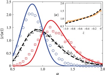
Comparison of steady-state particle size distributions for the model (curves) and the DEM simulation for the conditions in figure 2(b) (data points) in terms of spatially averaged concentrations in the bottom half
 $\left<c({\it\alpha})\right>_{b}$
(grey, blue online, ○) and top half
 $\left<c({\it\alpha})\right>_{t}$
(grey, red online, ▫) of the flow (see text). For the model,
 ${\it\Gamma}=175$
. The particles have an overall truncated log-normal distribution,
 $f({\it\alpha})$
, with
 ${\it\sigma}=0.3$
(3.8), as indicated by the dashed curve (model) and triangles (DEM, black, ▵). (Inset) Mean particle diameter as a function of depth for the model (black, dashed curve) and DEM simulation (light grey, orange, ▫). All DEM data are averaged between 30 and 60 s of simulated time, during which the system is in the fully developed segregated state shown in figure 2(b).

To compare results from the DEM simulation to the model, a subtle precaution is needed to ensure that the calculated
 $c(z,{\it\alpha})$
(from the model) and the measured
 $c(z,{\it\alpha})$
distributions are equivalent. Since the DEM simulation uses periodic boundary conditions in the streamwise direction instead of prescribed flux boundary conditions typical of an actual chute flow, the set of particles is fixed throughout the simulation. Consequently, the total distribution of particles by volume satisfies
 $$\begin{eqnarray}\int _{-1}^{0}c(z,{\it\alpha})\,\text{d}z=f({\it\alpha}).\end{eqnarray}$$
Hence, for the case of chute flow with periodic boundary conditions in the streamwise direction, we numerically solve (3.6) subject to (3.9) instead of (3.7). For the purposes of comparison between the model and simulation, particle concentrations are spatially averaged in the top and bottom halves of the chute as
 $$\begin{eqnarray}\displaystyle \left.\begin{array}{@{}c@{}}\displaystyle \langle c({\it\alpha})\rangle _{t}=2\int _{-1/2}^{0}c(z,{\it\alpha})\,\text{d}z,\\ \displaystyle \langle c({\it\alpha})\rangle _{b}=2\int _{-1}^{-1/2}c(z,{\it\alpha})\,\text{d}z,\end{array}\right\} & & \displaystyle\end{eqnarray}$$
where
 $\left<c({\it\alpha})\right>_{t}$
is the average concentration of particles in the top half of the domain and
 $\left<c({\it\alpha})\right>_{b}$
is the average concentration in the bottom half of the domain.
The model and the DEM simulation are compared in figure 3 for
 $\left<c({\it\alpha})\right>_{t}$
and
 $\left<c({\it\alpha})\right>_{b}$
. The model agrees remarkably well with the DEM simulation, given the simplicity of the model and the simplifying assumptions made for the chute flow. Smaller particles tend toward the bottom portion of the flowing layer while larger particles tend toward the top, consistent with the image in figure 2(b). The inset of figure 3 shows the depth profile of the mean particle size as measured from the simulation and predicted by the model. The local mean particle size
 $\langle {\it\alpha}\rangle$
agrees quite well through the entire depth of the flowing layer, with only slight deviations near the top and bottom boundaries of the flowing layer, perhaps due to differences between the assumed linear velocity profile and the actual slightly nonlinear velocity profile, the estimation of
 $S$
or the assumption of a constant value for
 $D$
. Nevertheless, the match between the model and DEM simulations is quite good for most of the flowing layer thickness, demonstrating the effectiveness of the approach.
3.3 Effects of
 ${\it\Gamma}$
and
$f({\it\alpha})$
in chute flow


With the validation of the theoretical model by DEM simulation, we now explore the relative effects of segregation and diffusion on the steady-state particle distribution by varying the dimensionless parameter,
 ${\it\Gamma}$
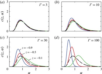
. Figure 4 shows
 $c(z,{\it\alpha})$
as a function of
 ${\it\alpha}$
at different depths in the domain for several values of
 ${\it\Gamma}$
. Particle sizes are distributed log normally according to (3.8) with
 ${\it\sigma}=0.4$
. At
 ${\it\Gamma}=3$
, the distributions at the top, middle and bottom of the domain are nearly identical to the overall particle size distribution
 $f({\it\alpha})$
(i.e.
 $c(z,{\it\alpha})\approx f({\it\alpha})$
), indicating that little segregation occurs. As
 ${\it\Gamma}$
becomes larger (less collisional diffusion), stronger segregation occurs. Near the bottom of the domain (
 $z=-0.9$
) there are mostly smaller particles (smaller
 ${\it\alpha}$
). Moving higher in the domain, there are fewer smaller particles, so the peak of the distribution shifts to the right. Moreover, toward the bottom of the flowing layer, the distribution of particle sizes becomes narrower, as evident in figure 4(d).
Steady-state probability density functions
 $c(z,{\it\alpha})$
for various
 ${\it\Gamma}$
at depths
 $z=-0.9$
(dark grey, blue online),
 $z=-0.5$
(grey, red online), and
 $z=-0.1$
(light grey, green online), showing increased segregation as
 ${\it\Gamma}$
increases: (a)
 ${\it\Gamma}=3$
, (b)
 ${\it\Gamma}=10$
, (c)
 ${\it\Gamma}=30$
, (d)
 ${\it\Gamma}=100$
. Particle sizes are distributed log normally according to (3.8) with the overall size distribution
 $f({\it\alpha})$
shown as a dashed curve.

Steady-state probability density functions
 $c(z,{\it\alpha})$
with an overall log-normal size distribution
 $f({\it\alpha})$
(dashed curve), for various
 ${\it\sigma}$
(see (3.8)) and
 ${\it\Gamma}=100$
: (a)
 ${\it\sigma}=0.2$
, (b)
 ${\it\sigma}=0.8$
. Here
 $z=-0.9$
(dark grey, blue online),
 $z=-0.5$
(grey, red online), and
 $z=-0.1$
(light grey, green online).

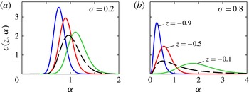
The effect of the variance
 ${\it\sigma}^{2}$
of the overall (log-normal) particle size distribution for
 ${\it\Gamma}=100$
is shown in figure 5. For small
 ${\it\sigma}$
, as in figure 5(a), particles are similar in size, so little segregation occurs. As
 ${\it\sigma}$
increases, segregation increases, and
 $c(z,{\it\alpha})$
varies substantially for different values of
 $z$
. For example, in figure 5(b),
 $c(-0.9,{\it\alpha})$
has much less spread than
 $c(-0.1,{\it\alpha})$
due to the long tail of the log-normal distribution. Thus, for large
 ${\it\sigma}$
, there is a wider range of large particle sizes (
 $1<{\it\alpha}<3$
) near the free surface.
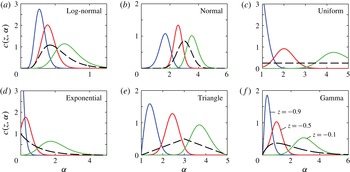
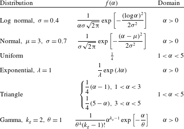
While log-normal particle size distributions are prevalent in many natural and industrial settings, other particle size distributions provide further insight into polydisperse segregation and demonstrate the broad applicability of our approach. In figure 6, six different distributions (summarized in table 1) are compared for
 ${\it\Gamma}=100$
at different depths in the domain. All six distributions have similar qualitative behaviour: small particles percolate toward the bottom of the flowing layer while large particles segregate toward the top.
Effect of different overall particle size distributions
 $f({\it\alpha})$
on steady-state probability density functions
 $c(z,{\it\alpha})$
for
 ${\it\Gamma}=100$
at
 $z=-0.9$
(dark grey, blue online),
 $z=-0.5$
(grey, red online), and
 $z=-0.1$
(light grey, green online): (a) log normal, (b) normal, (c) uniform, (d) exponential, (e) triangle, (f) gamma. The dashed curves represent
 $f({\it\alpha})$
. The six different overall particle size distributions are summarized in table 1. Note the different scales for each plot.

Particle size distributions considered in figure 6.

The log-normal and the normal particle size distributions in figure 6 generate segregated distributions
 $c(z,{\it\alpha})$
that are approximately log-normally and normally distributed, respectively, at each depth
 $z$
. For the uniform distribution and the exponential distribution, the segregated distributions are quite different at each depth. Near the bottom of the flow,
 $c(z,{\it\alpha})$
decays rapidly as
 ${\it\alpha}$
increases, and
 $c(z,{\it\alpha})$
has a maximum at
 ${\it\alpha}={\it\alpha}_{min}$
for both distributions. Conversely, near the middle or top of the flow,
 $c(z,{\it\alpha})$
is similar to a normal distribution. The triangular distribution results in segregated distributions similar to the normal distribution as well, except that
 $c(z,{\it\alpha})$
is skewed on different sides of the distribution at different depths, and
 $c(z,{\it\alpha})=0$
at
 ${\it\alpha}=1$
and
 ${\it\alpha}=5$
, since
 $f(1)=f(5)=0$
. The gamma distribution has a similar shape to the log-normal distribution, and thus
 $c(z,{\it\alpha})$
is similar for both distributions. Some of the overall size distributions in figure 6 exceed the range of applicability of the relation for the percolation length scale (2.3) but, as noted previously, the bulk of the particles are within the range of applicability, particularly at steady state.
Other particle size distributions can also be considered. Those depicted in figure 6 are only meant to give a flavour of the different particle segregation patterns possible and to demonstrate the potential that the modelling approach holds for describing other polydisperse mixtures.
4 Conclusion
This paper develops a continuum model for percolation-driven segregation of multidisperse and polydisperse granular material. The approach is effective in modelling multidisperse heap flow and polydisperse chute flow in that the spatial particle concentrations from theoretical predictions are consistent with those from DEM simulations. Several points are worth noting. First, the model does not rely on arbitrarily adjustable fitting parameters. Instead, the model uses general relations for the percolation velocity, diffusion and velocity profiles that can be based on theory, experiments, DEM simulations or any combination thereof. This permits the use of this approach across a wide range of granular flow geometries. Second, the model predictions seem relatively insensitive to uncertainties in determining the values for
 $S$
,
 $D$
and the velocity profile. This suggests that the approach can be broadly applied to a wide range of granular flows. Third, the approach can be applied to three-dimensional and unsteady flows if the kinematics of the flow are known. In fact, we have already applied the approach to transient bidisperse segregation in rotating tumbler flow (Schlick et al.
Reference Schlick, Fan, Umbanhowar, Ottino and Lueptow2015b
) and to steady-state bidisperse segregation in a three-dimensional conical heap (Schlick Reference Schlick2014). With the formulation of (3.1), these studies can be extended from bidisperse to polydisperse particle mixtures. Fourth, as we have explored in figures 1 and 6, any particle size distribution can be considered, whether multidisperse or polydisperse. This allows utilization of the approach to better understand how particle size distributions (maximum size ratio, standard deviations, etc.) affect segregation. Finally, while we have demonstrated the approach for size-disperse spherical particles, it can be readily adapted to other types of particle dispersity (e.g. density), provided that relations for the percolation velocity (2.3) and diffusion coefficient can be determined through experiment, theory, or DEM simulation.
The theoretical framework presented here for polydisperse size segregation in dense granular flow extends from a bidisperse segregation model by connecting key segregation parameters with particle and flow properties. The quantitative agreement between model predictions of polydisperse segregation and simulation results indicates this method has potential as a broadly applicable approach for modelling segregation in many types of polydisperse granular flows in industry and geophysics. To this point, the framework has been focused on modelling percolation-driven segregation – other segregation mechanisms in dense granular flow have not been considered, including density segregation (Khakhar, McCarthy & Ottino Reference Khakhar, McCarthy and Ottino1997; Tripathi & Khakhar Reference Tripathi and Khakhar2013), angle of repose-induced segregation due to particle shape or surface friction (Makse et al. Reference Makse, Havlin, King and Stanley1997) or shear-induced segregation due to shear rate gradients (Fan & Hill Reference Fan and Hill2011). These mechanisms can be incorporated into the framework by modelling each mechanism as a flux term similar to what we have done for the percolation-driven segregation flux. These extensions will complement the current model and move it further towards a general framework for modelling many types of particle segregation.
Acknowledgements
This research was funded by NSF grant CMMI-1000469 and The Dow Chemical Company. We thank K. Jacob for helpful discussions concerning polydisperse granular flows in industrial settings.