


INTRODUCTION
People’s assessment of how well their country is doing plays a critical role in many accounts of elections and political accountability. Valence outcomes (such as low unemployment, high economic growth, and low crime) are noticed by voters, who use those outcomes to evaluate officeholders, and thus affect incumbents’ electoral fortunes (Egan Reference Egan2013; Lenz Reference Lenz2012; Stokes Reference Stokes1963). The state of the economy stands out, both for the amount of research and for its consistent association with voters’ inclination to reelect the incumbent (see, among many others, Duch and Stevenson Reference Duch and Stevenson2008; Erikson, MacKuen, and Stimson Reference Erikson, MacKuen and Stimson2002; Fair Reference Fair1978; Healy and Malhotra Reference Healy and Malhotra2013; Kramer Reference Kramer1971).
Timing of valence outcomes plays an important role in key theories of elections, and different models place different emphases on past and future outcomes. In a sanctioning model (Ferejohn Reference Ferejohn1986), voters judge past outcomes to decide whether the incumbent deserves reelection. In selection models, voters aim to infer which candidate is most likely to deliver favorable conditions in the future (Alesina, Londregan, and Rosenthal Reference Alesina, Londregan and Rosenthal1993; Persson and Tabellini Reference Persson and Tabellini1994). According to selection models, past outcomes inform inferences about the incumbent’s competence to deliver benefits (Ashworth Reference Ashworth2012; Downs Reference Downs1957; Fiorina Reference Fiorina1981). Forecasts of future conditions and candidates’ proposals for creating favorable outcomes can also affect candidate selection (Fearon Reference Fearon, Przeworski, Manin and Stokes1999; MacKuen, Erikson, and Stimson Reference MacKuen, Erikson and Stimson1992; Stevenson and Duch Reference Stevenson and Duch2013).
Selection models in particular draw attention to another aspect of timing: whether conditions are improving. Improvement in the period leading up to an election could testify to the incumbent’s competence. Forecasted or proposed future improvements may be more attractive to voters than the prospect of stagnant or declining conditions. In retrospective assessments, a preference for improvement is difficult to distinguish from an overweighting of temporally proximate conditions, as both patterns involve a preference for maximizing positive outcomes as close as possible to the election. Noting that economic performance in the year or so before an election is particularly strongly associated with election-time economic evaluations and voting behavior, researchers have called the pattern “myopia” (e.g., Bartels Reference Bartels2008; Healy and Lenz Reference Healy and Lenz2014; Wlezien Reference Wlezien2015). This literature typically adopts the perspective of sanctioning models and views the disproportionate weighting of recent past performance as detrimental to electoral accountability, as voters neglect to consider economic performance earlier in the incumbent’s term when deciding whether to reward her with reelection (e.g., Healy and Malhotra Reference Healy and Malhotra2013). This could incentivize incumbents to prioritize policies with short-term benefits close to election years over more effective policies. In a selection model, in contrast, voters who overweight recent conditions or look for improvement in past outcomes might exert electoral accountability by responding to the incumbent’s competence.
Studying retrospective evaluations alone thus runs into an observational equivalence problem: under sanctioning models, overweighting recent conditions hurts accountability by disincentivizing an incumbent’s performance early in their term. Under selection models, overweighting recent conditions helps accountability by reelecting competent incumbents. We propose to separate these two interpretations by considering how voters should behave prospectively under the psychological presumptions implied by these interpretations. If retrospective myopia arises because people are short sighted, we should also see greater weight for conditions in the immediate future as opposed to several years later. If, on the other hand, people overweight the recent past because they value improvement, they should also reward improvement prospectively and not judge future trajectories based only on their immediate benefits.
In this article, we adjudicate empirically between preference for improvement and preference for temporally proximate benefits by comparing experimentally how people evaluate past and future conditions. In two different surveys, we replicate the pattern of retrospective myopia but observe the opposite, hyperopia, in prospection. For that reason, shorthand references to “myopia” (Bartels Reference Bartels2008), “myopic voting” (Healy and Lenz Reference Healy and Lenz2014, 44), and voters being “myopic” (Tufte Reference Tufte1978) are too general because they suggest higher valuation of temporally proximate benefits both backwards and forwards when in fact people take a longer view prospectively. Myopia remains descriptively accurate only when considering retrospective evaluations.
Our second goal in this article is to better understand the role of information about conditions in the early part of a time series. If retrospective assessments are myopic, early conditions receive little weight regardless of whether they are favorable or poor. This stands in contrast to the idea that people can use improving conditions as evidence that an incumbent is likely to produce greater future benefits. A voter assessing improvement does not disregard early conditions: between two trajectories with the same recent conditions, people prefer the trajectory that started with poor conditions to the one that starts with favorable conditions. In two more surveys carried out on four different samples, we find that respondents do in fact prefer trajectories that depict improving conditions, both retrospectively and prospectively.
The remainder of the article proceeds as follows. Part I explains the significance that evaluations of aggregate conditions have in theories of electoral choice and reviews existing research about empirical regularities. We then use two different research designs to examine myopia and preference for improvement in evaluations of aggregate conditions. Both designs randomly vary the “observed economy” (Stevenson and Duch Reference Stevenson and Duch2013) in a within-subject design to understand which series of economic conditions people prefer. Our study thus brackets the acquisition of information about the economy to focus on how people evaluate different economic trajectories. The approach covered in Part II presents respondents with information about conditions in the country and asks them to evaluate those conditions. Part III implements an alternative approach that uses a visual display with two trajectories of conditions in one graph, asking respondents to select the trajectory they prefer. Part IV uses an experimental strategy to show that preference for improvement partly reflects the heuristic appeal of upward trends but also involves a more considered assessment that improving conditions are desirable. In the conclusion, we discuss our findings in the context of theories of electoral choice.
PART I: AGGREGATE CONDITIONS IN THEORIES OF ELECTORAL CHOICE
Sanctioning and Selection Models
Aggregate conditions appear in different theoretical models of voter decision making—and play rather different roles. In a sanctioning model (Ferejohn Reference Ferejohn1986; Gieczewski and Li Reference Gieczewski and Li2024; Kramer Reference Kramer1971), voters (the principal) face a problem where agents (elected officials) might fail to generate voter welfare. Voters observe conditions in the country and use elections to sanction politicians by retaining them only if conditions are sufficiently good. In this model, conditions like the state of the economy indicate to voters whether the incumbent delivered. Voters use information about the past with the intention of evaluating past performance.
Selection models, in contrast, conceive of voters as trying to infer candidate type in order to support the candidate that is most likely to produce their preferred outcomes (Alesina, Londregan, and Rosenthal Reference Alesina, Londregan and Rosenthal1993; Duch and Stevenson Reference Duch and Stevenson2008; Fearon Reference Fearon, Przeworski, Manin and Stokes1999; Persson and Tabellini Reference Persson and Tabellini1994). While underlying type is unobservable, voters can use indicators such as past performance as a proxy to infer type and an incumbent’s ability to generate similar conditions in the future (Alesina, Londregan, and Rosenthal Reference Alesina, Londregan and Rosenthal1993; Downs Reference Downs1957; Fiorina Reference Fiorina1981). Here, past conditions inform voters’ inferences about the incumbent’s competence which is likely to influence conditions moving forward: “Voters look to the past to decide how to vote, but they do so from purely prospective motives” (Ashworth Reference Ashworth2012, 187) for “if voters are rationally seeking to influence their future welfare with their votes, then their retrospective judgment has a prospective purpose” (Fearon Reference Fearon, Przeworski, Manin and Stokes1999, 72).
Aggregate Conditions in Retrospective Voting
Retrospective voting based on aggregate conditions is consistent with both sanctioning and selection models. In a sanctioning model, the assessment of past conditions directly guides the choice to reelect the incumbent. In a selection model, people assess past conditions and then attempt to apportion to what extent they are due to the incumbent’s competence as opposed to nonpolitical shocks (Alesina, Londregan, and Rosenthal Reference Alesina, Londregan and Rosenthal1993; Duch and Stevenson Reference Duch and Stevenson2008). Evaluations of aggregate conditions are thus a foundational component of voter decision making. They are the first step in Healy and Malhotra’s (Reference Healy and Malhotra2013) four-step retrospective voting process and the first of two stages in Peress’s (Reference Peress2024) analysis of retrospective economic voting. Fiorina (Reference Fiorina1981) analyzed early American National Election Studies (ANES) questions that asked if people believed personal and aggregate conditions had gotten better or worse. Subsequent studies (e.g., Alvarez and Nagler Reference Alvarez and Nagler1998; Duch, Palmer, and Anderson Reference Duch, Palmer and Anderson2000; Kiewiet Reference Kiewiet1983; MacKuen, Erikson, and Stimson Reference MacKuen, Erikson and Stimson1992; Peress Reference Peress2024; Soroka, Stecula, and Wlezien Reference Soroka, Stecula and Wlezien2015) examined how such assessments relate to the objective indicators of economic conditions.Footnote 1
This article focuses on how people evaluate conditions in the country: presented with data about aggregate conditions, what patterns lead voters to conclude that conditions are favorable? Myopia could begin to affect the retrospective voting process starting at this early stage. Later steps in the process of retrospective voting build off of these evaluations (e.g., Healy and Malhotra Reference Healy and Malhotra2013) and involve attribution (beliefs about the extent to which officeholders are responsible for conditions) and vote choice (how much conditions attributed to the incumbent’s behavior matter relative to other aspects of the electoral choice). These steps are important in their own right and might also be subject to myopia or modify myopic evaluations of aggregate outcomes. For example, retrospective myopia could arise either because assessments of conditions are myopic or because the connection between assessments and vote choice has a shorter time horizon. We leave this question to future research in order to focus on the origins of myopic evaluations.
Myopia in Retrospective Voting
Myopia in retrospective voting has been demonstrated repeatedly, most prominently in judgments of economic performance, which are a key determinant of vote choice. When a US president is up for reelection, voters give much greater weight to economic conditions close to the election, and hardly any weight to the first half of the term, according to regressions of vote returns on economic indicators (Achen and Bartels Reference Achen and Bartels2016; Bartels Reference Bartels2008; Fair Reference Fair1978; Wlezien Reference Wlezien2015). Bartels (Reference Bartels2008, 98) concludes that “voters are myopic, responding strongly to income growth in presidential election years but ignoring or forgetting most of the rest of the incumbent administration’s record of economic performance.” Wlezien (Reference Wlezien2015, 201) agrees that “voters are myopic” but finds a longer time horizon with roughly equal weight of economic conditions in the two years preceding the election and little relevance of earlier conditions.
Evidence for the disproportionate impact of proximate economic conditions is not unanimous. In aggregate Swedish data, Healy, Persson, and Snowberg (Reference Healy, Persson and Snowberg2017) find evidence that voters place a larger weight on aggregate economic conditions in the most recent year before an election when casting their vote. However, when they instead use survey respondents’ tax returns to measure change in their disposable household income in each of the four years before the 2010 Swedish parliamentary election, the authors do not find a larger effect of income change in the years closer to the election compared to earlier years. They interpret this result as “inconsistent with a view of voters as suffering from a myopic bias” (782). Using Dutch and American individual-level panel data, Stiers, Dassonneville, and Lewis-Beck (Reference Stiers, Dassonneville and Lewis-Beck2020) show that economic evaluations several years before an election often have significant impact on incumbent (party) vote choice even when economic evaluations closely before the election are accounted for. They conclude that “voters are not fully myopic” (654).
Of particular relevance for our purposes is Healy and Lenz’s important Reference Healy and Lenz2014 study which presented survey respondents with economic data about the past, asked them to evaluate the strength of the economy depicted by those data, and found evaluations to be disproportionately driven by the most recent datapoints. Across multiple studies, Healy and Lenz (Reference Healy and Lenz2014) showed respondents a number of different charts with annual growth in real disposable income over four years. Below each chart, respondents were asked to evaluate the depicted economy: “How would you rate the condition of the national economy during this period? Is it very good, fairly good, fairly bad, or very bad?” To estimate the importance of economic performance in different years, the authors regressed respondents’ summary evaluations of the economy on each year’s income growth as presented in the graphs. The results (including a replication in Healy, Persson, and Snowberg Reference Healy, Persson and Snowberg2017) consistently show greater regression coefficients for years closer to the election. Because respondents see the economic data just before they rate the economy (on the same screen), this design demonstrates that retrospective myopia is not (exclusively) a product of limited memory.
Healy and Lenz deliberately designed their experiments to minimize the possibility that incumbent-related considerations might color economic evaluations and produce myopia—focusing their theory on the evaluation of aggregate conditions stage. Most of their surveys told respondents that the income growth statistics were for hypothetical incumbent presidents in their second terms, thus reducing reelection considerations and evaluations tied to a specific incumbent, and asked respondents to evaluate the economy, as opposed to the incumbent’s handling of the economy. Healy and Lenz demonstrate the robustness of their findings when presidents, and politics generally, are not mentioned in the experiments (see Healy and Lenz’s Study C2).Footnote 2
Aggregate Conditions in Prospective Voting
According to both selection models and theories of economic voting, voters do not ignore the future when they consider their vote choice. Selection models posit that voters evaluate aggregate conditions to discern candidates’ types and their potential to bring about favorable conditions in the future. In doing so, they may rely on past (actual) or future (projected or proposed) conditions. Research on economic voting has related leading economic indicators (past conditions that tend to forecast future conditions) to aggregated economic perceptions and expectations, such as survey questions from the Survey of Consumer Attitudes. Leading economic indicators are associated with economic expectations measured in surveys and with aggregate political outcomes such as election results, suggesting that the public prospectively evaluates the economy (e.g., Duch and Stevenson Reference Duch and Stevenson2011; Erikson, MacKuen, and Stimson Reference Erikson, MacKuen and Stimson2002; MacKuen, Erikson, and Stimson Reference MacKuen, Erikson and Stimson1992; Soroka, Stecula, and Wlezien Reference Soroka, Stecula and Wlezien2015).
Although past performance and forecasts based on past conditions might be more reliable guides when inferring candidate competence, selection models also include prospective issue voting among the tools that voters might use to infer candidate type and make political decisions (Fearon Reference Fearon, Przeworski, Manin and Stokes1999; Fiorina Reference Fiorina1981). According to Fearon (Reference Fearon, Przeworski, Manin and Stokes1999, 60), “voters trying to select good types from campaign speeches face the problem of noisy and misleading signals, but informative signaling is not a priori impossible.” Future-oriented consideration of past performance hinges on observing actual conditions, whereas issue voting involves information about conditions that have not yet materialized. These could be proposals of aggregate conditions made by candidates themselves (platforms) or independent projections of aggregate conditions if the incumbent stays in office (such as media reports of economic forecasts; see Stevenson and Duch Reference Stevenson and Duch2013).
Although political science has almost exclusively studied retrospective myopia, prospective evaluations, too, may be affected by myopia. In many other contexts, the term “myopia” in fact refers to short time horizons in evaluations of the future.Footnote 3 If people have a general tendency to value temporally proximate benefits more highly than temporally distant benefits, we should see myopia in prospection as well. To understand if prospective assessments of aggregate conditions are also myopic (so that people consider predictions of future outcomes but give the greatest weight to the immediate future), we first replicate Healy and Lenz’s finding that evaluations of past aggregate conditions are myopic, and then apply the same research design to future conditions. According to the Universal Myopia Hypothesis, a narrow focus on temporally proximate conditions underlies retrospective myopia and produces myopia in prospection as well.
Preference for Improvement
Rather than narrowly focus on temporally proximate conditions, people may instead aim to discern competence by assessing improvement in conditions. Preference for improvement is different from myopia (and hyperopia) because it implies that people care about conditions throughout the trajectory and prefer those conditions to improve over time. Studies in psychology show that people are willing to endure poor outcomes now if it means better outcomes in the future (e.g., Loewenstein and Prelec Reference Loewenstein and Prelec1993). People prefer good outcomes to increase over time (Zauberman, Diehl, and Ariely Reference Zauberman, Diehl and Ariely2006) and bad outcomes to decrease (Varey and Kahneman Reference Varey and Kahneman1992). For example, holding constant lifetime earnings, people prefer their earnings to increase over time rather than decrease or remain constant (Read and Powell Reference Read and Powell2002).
There is also a role of improving conditions in the economic voting literature, through “benchmarking,” the claim that people use the relative rather than absolute state of the economy to judge incumbents (e.g., Arel-Bundock, Blais, and Dassonneville Reference Arel-Bundock, Blais and Dassonneville2021; Aytaç Reference Aytaç2018; Soroka, Stecula, and Wlezien Reference Soroka, Stecula and Wlezien2015).Footnote 4 This research is often conducted at the aggregate level by regressing incumbent vote share on (absolute or relative) economic conditions, so theory presumes that voters have information about the earlier reference point, an assumption that Arel-Bundock, Blais, and Dassonneville (Reference Arel-Bundock, Blais and Dassonneville2021) called into question. Political actors and media do provide information on changing conditions (Soroka, Stecula, and Wlezien Reference Soroka, Stecula and Wlezien2015; Stevenson and Duch Reference Stevenson and Duch2013). Our research design presents respondents with trajectories of past conditions, so we bracket the issue of memory and examine if preference for improvement affects evaluations of known aggregate conditions. According to our Universal Preference for Improvement Hypothesis, people prefer conditions that involve a build-up to greater benefits over time—regardless of whether they are evaluating past or future conditions.
Cognitive Bias or Genuine Preference?
Both universal myopia and universal preference for improvement may emerge from a cognitive bias induced by the visual presentation of data over time. For example, Healy and Lenz (Reference Healy and Lenz2014) demonstrate that retrospective myopia is attenuated (though not eliminated) when respondents are also shown cumulative outcomes over the entire time period. Similarly, Prior and Andrews (Reference Prior and Andrews2025) demonstrate that preference for upward trends is reduced (though not eliminated) when respondents are discouraged from extrapolating beyond the data.
To distinguish genuine preferences from cognitive bias induced by the heuristic appeal of visual presentations, we randomly assign debiasing presentations of data to some respondents. These treatments combine both Healy and Lenz’s idea of adding cumulative outcomes to the data presentation and Prior and Andrews’ treatment to discourage extrapolation beyond the data. This design allows us to examine the Universal Preference for Improvement Hypothesis in two different conditions: first, when sequences of noncumulated conditions invite heuristic biases, and, second, when presentation attenuates these biases.
Plan of Analysis
Each of the following empirical sections begins with a description of the research design, then presents the results of experiments that randomly assign participants to consider past or future conditions (for replication data, see Prior and Andrews Reference Prior and Andrews2026). Our experiments are embedded in four different opinion surveys, conducted on several different platforms between the fall of 2020 and the spring of 2022. We draw on MTurk samples from October 2020 (Survey A), March 2021 (Survey B), December 2021 (Survey C), and May 2022 (Survey D).Footnote 5 Survey C was also fielded on a second opt-in platform, Volunteer Science,Footnote 6 and permits direct comparison of the two convenience samples. We also ran Survey D on a probability sample administered by NORC. Compared to the Current Population Survey (CPS), the opt-in samples have too few non-whites and people without high-school degrees, and too many college graduates. VS overrepresents people over 50, whereas MTurk underrepresents them. NORC matches CPS benchmarks closely even before weighting (see Appendix A of the Supplementary Material for demographics). NORC estimates are weighted (applying base, non-response, and post-stratification weights).
Part II, which investigates myopia and preference for improvement, draws on Surveys A and B. Part III introduces a choice-based measurement design of preference for improvement and implements it in Surveys C and D. Part IV uses Survey D to examine to what extent myopia and preference for improvement result from uncritical cognitive biases or reflect considered assessments of aggregate conditions.
PART II: RATINGS OF AGGREGATE CONDITIONS
Research Design
Stimulus Creation and Presentation
The stimulus plots describing aggregate conditions in Part II closely resemble the presentation format in Healy and Lenz (Reference Healy and Lenz2014). In all but one of their surveys, Healy and Lenz showed respondents charts with randomly generated annual growth rates drawn from a normal distribution with mean of 2% real disposable income (RDI) growth and standard deviation of 2, roughly the distribution of annual growth in the United States from 1948 to 2008. The method creates yearly values that are independent from each other in expectation, which facilitates the estimation of annual weights. The downside for our purposes—understanding the effect of improving or deteriorating conditions—is the large share of nonmonotonic sequences (sequences with both ups and downs) created by this sampling approach.
To generate more monotonic trends and sequences with the same values arranged nonmonotonically, we stratified our sampling approach. In Survey A, we draw four values from the historical distribution of RDI growth to create a monotonically increasing plot by putting them in ascending order and a monotonically decreasing plot that displays the same values in descending order. Two additional plots systemically switch some values to create nonmonotonic sequences. The advantage is that each set of sequences created this way holds constant total growth over the entire period, thus balancing on an alternative characteristic of conditions that might affect evaluations. The downside is that this method of creating stimulus plots induces some correlations between annual values (leading to efficiency loss in models that use all annual values as separate regressors). Appendix B of the Supplementary Material provides details on how we generated plots for each of our surveys.
Survey B covered environmental conditions and randomly varied whether conditions were described as “air quality” or “air pollution” to extend our investigation into the loss domain. Both conditions presented respondents with plots using a modified air quality index (AQI) with a range of 0–1000.Footnote 7 The scale maintains the five levels of severity and corresponding colors from the actual AQI but recasts them into equal-sized segments of 200 units each. In the air pollution version (as well the original AQI), large numbers indicate cleaner air; the air quality condition flips scale orientation. These modifications of the AQI allow us to compare results for costs and benefits while holding everything else constant.
Survey B uses a similar stratified sampling approach as Survey A to generate monotonic trends. We create monotonically increasing sequences with varying the slopes while maintaining similar averages across each sequence. We flipped the values to generate otherwise similar sequences with decreasing slopes. This process is repeated twice, using two different averages. Respondents were also presented with non-monotonic sequences, with values randomly drawn from the values used in the monotonic sequences to keep the averages the same (see Appendix B of the Supplementary Material for details).
In Survey A, respondents evaluated 16 plots per module. Each module included three sets of four sequences that each balance on trend and average growth. An additional four sequences were randomly drawn. Modules in Survey B consisted of 18 plots. Each module had four sets of plots, each of which varied a given trend in minor ways, so balancing of trends occurs across sets in this survey, while averages are held approximately constant within sets. Two of the four randomly drawn plots completed each module.
Experimental Designs
The main experimental manipulation throughout this study involves presenting the same conditions as either past or future. The Past treatment asks respondents “to imagine you are looking backward at past economic growth over a four-year period” (Survey A) and to evaluate conditions after seeing “different measurements of air quality over the past few years” (Survey B). To increase ecological validity, the Future treatment describes conditions as proposals of future conditions (Survey A) or “scenarios” (Survey B), rather than certain outcomes. This introduces the possibility that respondents will not just evaluate the proposal itself, but its feasibility and certainty. We alleviate this concern by removing any mention of politicians or officeholders trying to achieve this proposal so that the competence of any specific politician will not influence evaluations. This design follows Healy and Lenz’s Study C2, which removed all mentions of politics (and replicated retrospective myopia). Previous experimental evidence shows that hypothetical policy proposals are an effective way to manipulate participants’ expectations for the future (Malhotra and Margalit Reference Malhotra and Margalit2014).
In Survey A, respondents were randomly assigned to see one or two plot modules within the survey. Respondents who saw one plot module finished a second module (not involving plots) of similar length which included a different instrument to evaluate economic conditions. In Survey B, all respondents were asked to complete two modules of plot evaluations. Module order and time orientation were always randomized. Statistical models control for module order.
For the experimental design to succeed, it is critical that respondents understand the time orientation of the conditions they are evaluating. To accomplish this objective, we used highlighting, repetition, and verbal reminders with each plot. In the instructions for Survey A, respondents were told, “we would like you to imagine you are looking backward at past economic growth over a four-year period,” or “forward at proposed economic growth over a four-year period,” (emphasis retained from survey). Before beginning the task, they were reminded again that they were either considering past or future proposed growth, and the evaluation question prompted respondents to consider either the past or future. In Survey B, respondents were given similar reminders throughout the instructions and were asked to evaluate the air quality either during the past or future period. We designed the plots to serve as an additional reminder. The survey was conducted in March of 2021, and rather than presenting respondents with plots with an x-axis labeled from “Year 1” to “Year 4,” in the past condition they instead were labeled “February 2018” through “February 2021.” In the future, they were labeled from “April 2021” through “April 2024.” Instructions for plot evaluations in Surveys A and B appear in Appendix C of the Supplementary Material.
Surveys included manipulation checks after each module asking respondents if the questions they just answered referred to the past or future (see Appendix E of the Supplementary Material). In Survey A, 95% of respondents in the Past condition and 86% in the Future condition passed the manipulation check. In Survey B, at least 98% of respondents passed in each time orientation and domain. The large majority of respondents thus understood the time orientation. In order to avoid post-treatment bias, analyses include respondents regardless of how they did on the manipulation checks (Berinsky, Margolis, and Sances Reference Berinsky, Margolis and Sances2014).
Outcome Measures
At the bottom of each screen showing a plot, respondents were asked to evaluate the conditions depicted. The Survey A prompt was “How would you rate the condition of the [past/future] national economy during this period? Very bad, fairly bad, fairly good, or very good?” The four-point scale follows Healy and Lenz (Reference Healy and Lenz2014); we rescale it to 0–10 for analysis. Survey B used a 0–10 scale: “How would you rate air [quality/pollution] during this [past/future] period? Please answer on a scale from 0 to 10, where 0 means very bad and 10 means very good.”
Results
People consistently give more weight to recent datapoints in evaluations of retrospective conditions. Using similar empirical designs that vary a number of features for robustness, Healy and Lenz (Reference Healy and Lenz2014) show this pattern for economic conditions and crime (their SI, 16), and we replicate it for economic conditions and extend it to environmental conditions. In the first column for each domain, Table 1 shows the familiar pattern of little weight for early years and the largest weight for the most recent year when looking to the past. (Survey A averages income growth over the first two years because our random draws produced too high a correlation between Year 1 and Year 2.)Footnote 8
Effect of Annual Statistics on Evaluations of Aggregate Conditions
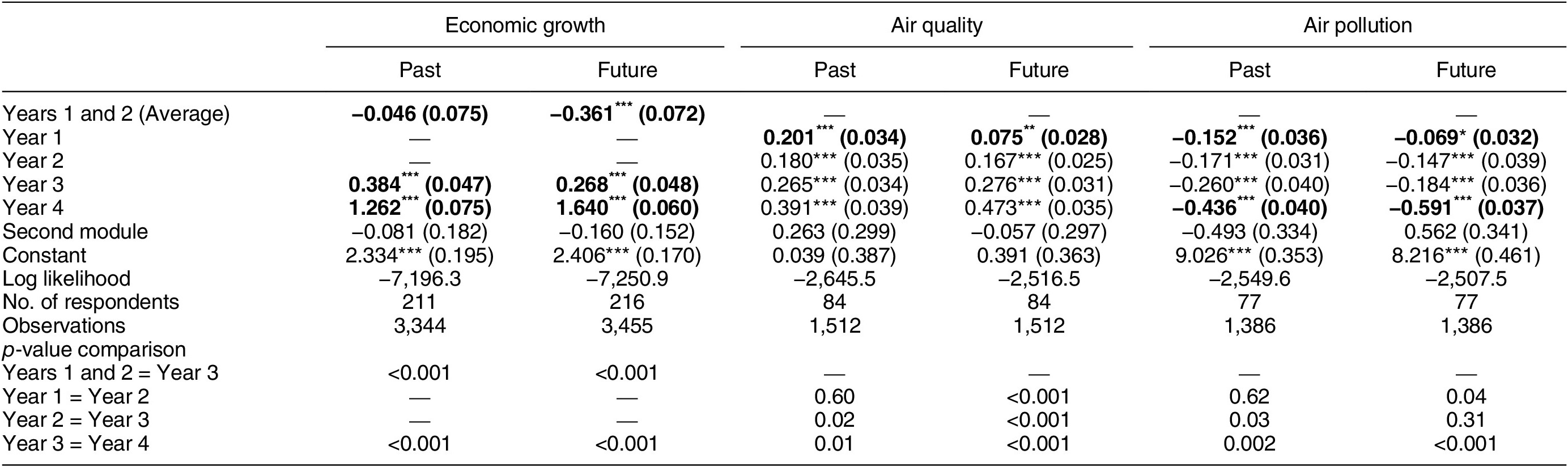
Table 1. Long description
The table is organized into six data columns under three main headings: Economic growth, Air quality, and Air pollution, each split into Past and Future evaluations.
* Economic growth:
- Years 1 and 2 (Average): Past -0.046 (0.075); Future -0.361*** (0.072).
- Year 3: Past 0.384*** (0.047); Future 0.268*** (0.048).
- Year 4: Past 1.262*** (0.075); Future 1.640*** (0.060).
* Air quality:
- Year 1: Past 0.201*** (0.034); Future 0.075** (0.028).
- Year 2: Past 0.180*** (0.035); Future 0.167*** (0.025).
- Year 3: Past 0.265*** (0.034); Future 0.276*** (0.031).
- Year 4: Past 0.391*** (0.039); Future 0.473*** (0.035).
* Air pollution:
- Year 1: Past -0.152*** (0.036); Future -0.069* (0.032).
- Year 2: Past -0.171*** (0.031); Future -0.147*** (0.039).
- Year 3: Past -0.260*** (0.040); Future -0.184*** (0.036).
- Year 4: Past -0.436*** (0.040); Future -0.591*** (0.037).
* Model Statistics:
- Log likelihood ranges from -7,196.3 (Economic growth Past) to -2,507.5 (Air pollution Future).
- Number of respondents: 211-216 for Economic growth, 84 for Air quality, and 77 for Air pollution.
* p-value comparisons:
- Year 3 vs Year 4 comparisons are all significant at p < 0.001 across all categories.
- Year 1 vs Year 2 is significant for Future Air quality (p < 0.001) and Future Air pollution (p = 0.04).
Note: * p < 0.05, ** p < 0.01, *** p < 0.001. The table shows coefficients from a linear hierarchical model with individual random effects and heterogeneous residual variances. Standard errors are shown in parentheses. Air quality and pollution enter in 100s of scale units. Bolded coefficients are significantly different at p < 0.05 between past and future.
The second column for each domain presents the estimated weights for conditions under the Future treatment to test the Universal Myopia Hypothesis. Myopia in prospection would manifest in the largest weights for the most temporally proximate conditions when looking forward. Table 1 clearly and consistently shows the opposite pattern: people’s evaluations of future economic and environmental conditions are disproportionately shaped by conditions later in the time period. In fact, Year 4 tends to matter even more in prospection than retrospection. This result complements the demonstration by Prior, Alsharawy, and Andrews (Reference Prior, Alsharawy and Andrews2023) that temporal discounting is greater in retrospection than prospection. Whereas our study uses the operationalization of myopia common in political science, Prior, Alsharawy, and Andrews used an entirely distinct measurement strategy originating in behavioral economics that is choice-based and does not involve graphical presentation of data.
Judging aggregate conditions so disproportionately by the later datapoints in prospection is notable for a different reason than in retrospection. Behavioral economics and psychology often describe people as overly concerned with immediate outcomes and giving too little weight to their own future welfare. Table 1 appears to show the opposite: hyperopia. A possible explanation focuses on people’s preference for conditions to improve. Preference for improvement is different from hyperopia because it implies that people do care about the immediate future and, counterintuitively, prefer to start with relatively poor conditions that subsequently improve. The models in Table 1 do not pick this up because they assess the impact of each datapoint separately. Diagnosing improving conditions requires a starting point, so the statistical model needs to examine the impact of later datapoints relative to earlier datapoints—that is, assess the impact of trends.
Healy and Lenz (Reference Healy and Lenz2014) briefly investigated whether trends affect evaluations. In analyses reported in their SI (23), they add indicator variables for monotonically increasing and decreasing sequences among their 125 different plots (pooling five studies). These variables have significant effects while leaving the annual weights pretty much unchanged. Their examination of trends in randomly generated growth data is limited by the small number of plots with clear trends and by interdependence of plot properties, however. Among the 125 growth plots, only 7% have monotonic upward trends and 6% have monotonic downward trends. Moreover, conditional on the average of the sequence, the trend (defined as end value minus start value) and endpoint of a sequence are not independent. Average annual growth is 1.2 points (almost 60%) higher for increasing sequences than for sequences without consistent trend. Presence of an upward trend correlates at 0.43 with Year 4 growth.
We purposefully designed our studies to estimate the impact of trends. The stratified sampling approach we used to populate plots with data yields a larger number of monotonic sequences. To guard against demand characteristics, we still included some randomly populated plots that fit the design principles used by Healy and Lenz. Our first test of the impact of trends uses all plots (and thus the same data as the models in Table 1). Figure 1 shows predicted evaluations for each plot based on a regression model that controls for the average conditions shown by the plot, its time orientation, and whether the plot was part of the first or second survey module. The horizontal axis notes the slope of the plot, defined as the difference between last and first datapoint. Coverage on the x axis is irregular in Survey A because the slopes of randomly populated plots are themselves random. Survey B includes two versions of the non-monotonic plots with opposite (and shallow) slopes, so the distribution of slopes is symmetrical around zero.
Evaluations of Aggregate Condition, by Slope and Time Orientation
Note: Graphs show coefficients from hierarchical regression models that hold constant the average of conditions. Point estimates are predicted values, and error bars are 95% confidence intervals. Full results appear in Tables F1 and F2 in the Supplementary Material.
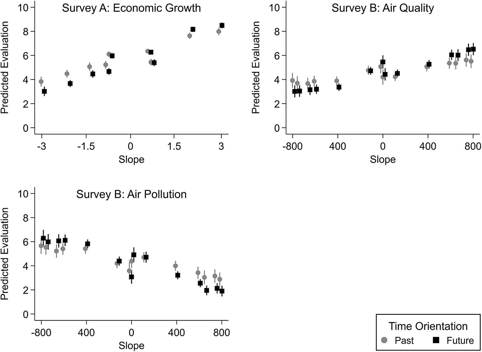
Figure 1. Long description
A multi-panel figure containing three scatter plots. All plots share a Y axis labeled Predicted Evaluation ranging from 0 to 10. A legend at the bottom right identifies gray circles as Past and black squares as Future.
* Top-left plot: Survey A: Economic Growth. The X axis is Slope ranging from -3 to 3. Both Past and Future data points show a strong positive linear correlation. As slope increases from -3 to 3, predicted evaluation rises from approximately 3 to 8.5.
* Top-right plot: Survey B: Air Quality. The X axis is Slope ranging from -800 to 800. Both data series show a moderate positive linear trend. Predicted evaluations start around 3 at a slope of -800 and rise to approximately 6.5 at a slope of 800.
* Bottom-left plot: Survey B: Air Pollution. The X axis is Slope ranging from -800 to 800. Both data series show a negative linear trend. Predicted evaluations start near 6 at a slope of -800 and decrease to approximately 2 at a slope of 800.
In all plots, point estimates are accompanied by vertical error bars representing 95 percent confidence intervals.
Figure 1 shows that plots with more positive slopes tend to receive more favorable evaluations, controlling for average conditions over the charted time period. This effect persists regardless of whether people evaluate the past or the future. The fit between slope and evaluation deviates from a simple linear relationship, especially in Survey A and for the plots in Survey B with near-zero slopes. This is likely because slope and average do not comprehensively define plots, and differences in evaluations arise due to other features (sometimes referred to as “gestalt” in the literature on sequences; see Ariely and Carmon Reference Ariely and Carmon2000). We did not constrain all plots to be monotonic, and even monotonic sequences can have different inflection points (local slopes). The plots with near-zero slopes in our design are nonmonotonic, introducing peaks and troughs that likely also shape evaluations. The main advantage of stratified sampling in populating plots is that we can hold constant additional plot features by using only balanced plots.
To estimate the effect of trends without having to control for variation in other correlated characteristics we turn to a subset of the plots in our data. In Survey A, we retain 12 plots: three sets of four plots, one increasing, its decreasing mirror image, and the final two plots comprised of the same values but in a randomized order such that they are nonmonotonic and have a slope close to zero. The design achieves balance across averages (all plots in a set are the same) and slopes (each set contains approximately the same slopes). In Survey B, we retain eight plots: one is increasing, its mirror image, and two nonmonotonic plots with the same average and slopes near zero.Footnote 9 Relying on this approach means we are drawing comparisons between increasing, decreasing, and no trend plots with identical total benefits over the shown time-period.
Figure 2 presents the results of this more design-based analysis of slope effects. Trajectories with increasing trends receive substantially and significantly higher evaluation in every test in Figure 2. This confirms our Universal Preference for Improvement Hypothesis: trends operate similarly in retrospection and prospection because people value improvement in conditions regardless of whether they are assessing the past or the future.
Evaluations of Balanced Conditions, by Slope and Time Orientation
Note: Graphs show coefficients from hierarchical regression models that hold constant the average of conditions. Point estimates are predicted values, and error bars are 95% confidence intervals. Full results appear in Tables F3 and F4 in the Supplementary Material.
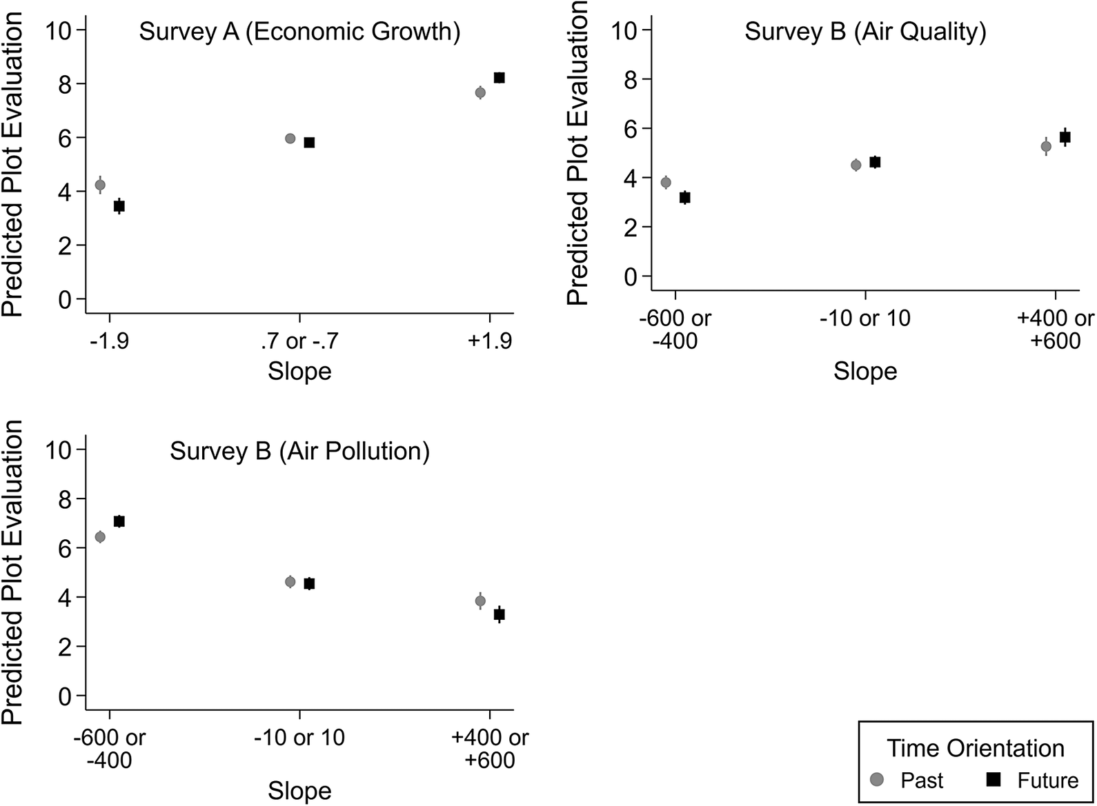
Figure 2. Long description
A multi-panel figure with three scatter plots. All plots share a Y-axis labeled Predicted Plot Evaluation ranging from 0 to 10 and an X-axis labeled Slope. A legend at the bottom right identifies grey circles as Past and black squares as Future.
* Top-Left Panel: Survey A (Economic Growth). At slope -1.9, Past is approximately 4.2 and Future is 3.5. At slope .7 or -.7, Past and Future are both near 6. At slope +1.9, Past is 7.8 and Future is 8.2. The trend shows a positive linear increase.
* Top-Right Panel: Survey B (Air Quality). At slope -600 or -400, Past is 3.8 and Future is 3.2. At slope -10 or 10, Past and Future are near 4.5. At slope +400 or +600, Past is 5.2 and Future is 5.8. The trend shows a slight positive linear increase.
* Bottom-Left Panel: Survey B (Air Pollution). At slope -600 or -400, Past is 6.5 and Future is 7.1. At slope -10 or 10, Past and Future are near 4.5. At slope +400 or +600, Past is 3.9 and Future is 3.3. The trend shows a negative linear decrease.
All data points include vertical error bars representing 95 percent confidence intervals.
Even using only plots with slopes balanced around the same average benefits, these analyses cannot determine whether the trend or the endpoint of conditions is more important for evaluations—conditional on the average, they are not independent of each other. Instead, our results clearly show that trends affect evaluations. This conceptually distinguishes a preference for improvement from retrospective myopia (and prospective hyperopia) as causes of people’s assessments of aggregate conditions. Systematic effects of trends imply that people do not jump to conclusions by focusing only on the more recent conditions—change in conditions is an important determinant of their evaluations.
There is no evidence that the style of plots affects conclusions about myopia, hyperopia, or preference for improvement. Healy and Lenz (Reference Healy and Lenz2014, SI, 14) show robustness to vertical plots. In the pollution condition of Survey B, we randomly assigned respondents to either bar plots (the style used in Survey A and for air quality) or line plots with either four or seven datapoints. Respondents show preference for improvement across in all plot styles under both Past and Future conditions (see Table F5 and Figure F1 in the Supplementary Material).
PART III: PREFERENCE FOR AGGREGATE CONDITIONS
Preference for improvement in prospection is striking because it so clearly contradicts the idea that people are focused on the immediate future. This section boosts the robustness of this finding in four ways. First, it introduces a choice-based approach where respondents pick the conditions they prefer from two options shown in the same graph. This drops the assumption that people are able to meaningfully compare trajectories presented in separate graphs on separate survey screens. Second, the choice-based approach systematically varies the average of the depicted conditions but holds other plot characteristics constant. Third, this section quantifies more precisely the results in Part II that people are willing to sacrifice sooner benefits for a more lasting improvement in conditions. Our choice-based method gauges how good conditions without improvement have to be to make people indifferent to a trajectory that improves by a particular amount. Fourth, this section uses a probability-based sample of US residents to make sure that preference for improvement generalizes to the population.
Research Design
Adaptive Measurement of Preference for Improvement
To calibrate the extent to which people are willing to sacrifice overall welfare for increasing trends, we implemented an adaptive measurement approach that asked respondents to repeatedly choose between two sequences plotted in the same graph which differ from each other in slope and average (see Andrews, Curl, and Prior Reference Andrews, Curl and Prior2026). Depending on which sequence a respondent prefers, the next graph increases or decreases the average of the flat sequence. After four iterations, the adaptive approach pinpoints the average of the flat sequence that makes respondents indifferent between the two sequences, revealing how much higher (or lower) the average of the flat sequence must be for a respondent to accept it in exchange for a specific increasing trend. We apply this method in the domain of personal income growth and temporary job creation in the United States.
More specifically, respondents are presented with a plot that includes a flat and a rising sequence and asked to mark the one they prefer. Next, we show respondents another plot that adjusts the flat sequence depending on their previous choice and asks them to pick again between the same increasing slope sequence and the adjusted flat sequence. If a respondent selects the rising (flat) sequence, we increase (decrease) the average of the flat sequence. In other words, the adaptive method makes the flat sequence more appealing for respondents who previously preferred the rising sequence. And it makes the flat sequence less appealing if respondents already preferred the flat sequence. The size of the adjustment halves with each adaptive step. For each respondent who does not always select the same answer, this identifies the interval bounding the indifference point where the respondent switched between the flat and rising sequences. We take the midpoint of the “switching” interval as the indifference point and use it as a measure of preference for improvement.Footnote 10 Figure D1 in the Supplementary Material illustrates the method.
When the average of the flat sequence is greater than the average of the rising sequence, respondents are willing to sacrifice overall welfare in exchange for improving conditions during the time period. The difference between averages of the two sequences calibrates preference for improvement in outcome units. It describes how much less of the outcome, in the units of the outcome, a respondent is willing to accept in return for the particular improvement shown by the rising sequence. The calibration is necessarily relative to the sequence properties that are fixed across adaptive steps. The fixed rising trajectory averaged to income growth of 2.1% per year in Survey C and 1.3% per year in Survey D. The fixed sequence depicting job creation showed 243,750 jobs per year. Because we designed both lines in the plot to be highly similar in shape other than its slope, this method holds constant more characteristics of the data presentation than the approach in Part II.
Experimental Design
As in Part II, the key manipulation is the plot’s time orientation. In Surveys C and D, all respondents completed the adaptive instrument twice, once choosing between plots illustrating past conditions and once choosing between future projections. The order was randomized. We also manipulated the domain in which respondents evaluated sequences. In Survey C, respondents were recruited via MTurk (N = 1,181) or Volunteer Science (VS, N = 437) and evaluated plots of RDI growth, the same economic indicator as in Survey A. In Survey D, respondents were recruited via MTurk (N = 833) or NORC (N = 2,321). All MTurkers evaluated plots of income growth over four years. NORC respondents were randomly assigned to evaluate income growth or job creation. For the latter, the survey explained that “Temporary jobs are created when employees take short-term (1-year) contracts. They are beneficial to both job candidates and employers.”
Instrument design ensured that participants understood whether they were evaluating past or future conditions. The instructions distinguished the two verbally and by using different colors for references to past and future. Survey D, for example, explained the task about “[past/future] income growth” as showing “two [histories of growth/two growth projections].” After each plot, the participants were asked, “Which of these two [histories/projections] of income growth do you think is better?” Words in brackets appeared in distinct colors. Like in Survey B, plots also included dates on the x-axis. For Survey D, which was conducted in 2022, dates ranged from 2019 to 2022 in the Past condition and 2022 to 2025 in the Future condition. These design features appear successful: in Survey C, 93% (Future) and 82% (Past) correctly identified the time orientation of the plots in a post-treatment manipulation check on MTurk. 92% (Future) and 78% (Past) of respondents on VS did the same. Respective percentages in Survey D were 91% (Future) and 72% (Past) for MTurk and 90% (Future) and 60% (Past) for NORC.Footnote 11 The results we report in the next section are substantially unchanged when we only include participants who passed the manipulation check (see Appendix G of the Supplementary Material).
Results
Figure 3 presents the distributions of preference for improvement from our different samples and domains. The dashed vertical line indicates the average benefit under the fixed, improving conditions. Values to the right of this line represent respondents who require more benefits in the flat sequence than the rising sequence to be indifferent between flat and rising conditions—that is, they are willing to sacrifice overall benefits for improving conditions. This describes a large majority of respondents in all 10 distributions plotted in Figure 3. Legends to each panel show mean and median of each distribution. Drawing on our probability-based NORC sample, the results in Figure 3C show that the average US resident needs to see at least 2.3% of economic growth per year to prefer constant growth rates to a trajectory of improving conditions with only 1.3% annual growth. NORC respondents who completed the adaptive measure for job creation prefer improving conditions that generate on average 243,750 jobs per year unless the flat conditions deliver at least 350,000 jobs per year. The identical instrument produces very similar results on the MTurk sample run at the same time.
Choice-Based Preference for Improvement, by Time Orientation
Note: Graphs plot distributions of indifference points with a fixed sequence without an evident slope (marked by the dashed vertical line). Means (μ) and medians (M) are scaled in substantive units. Tests of equality cluster at respondent level to account for repeated observations. NORC data apply sampling and post-stratification weights.
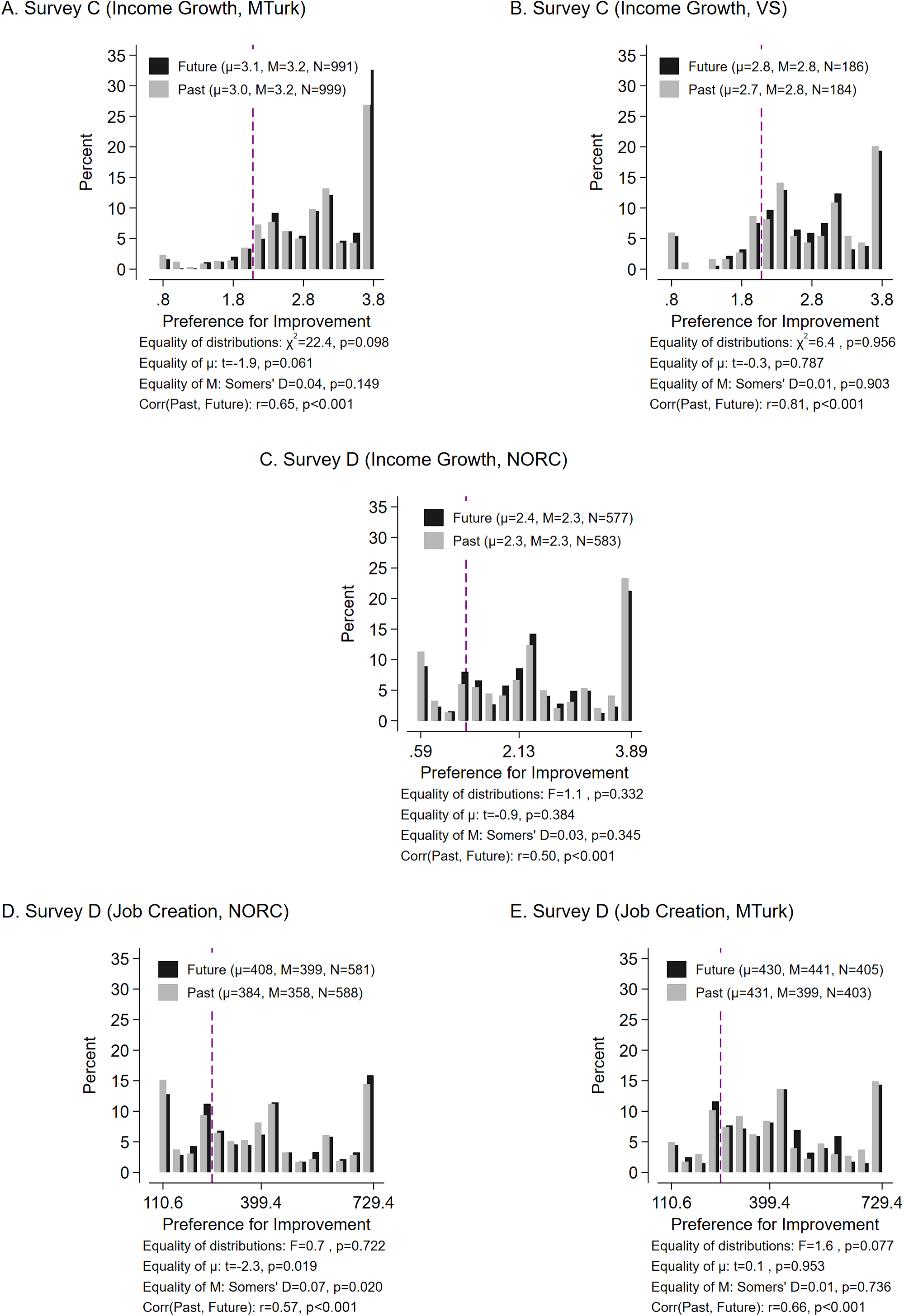
Figure 3. Long description
The figure consists of five panels labeled A through E. Each panel is a bar chart with the Y-axis representing Percent from 0 to 35 and the X-axis representing Preference for Improvement. Each chart compares two groups: Future (black bars) and Past (gray bars). A dashed vertical line marks the indifference point in each plot.
* Panel A. Survey C (Income Growth, M Turk): X-axis ranges from .8 to 3.8. Data shows a significant peak at the rightmost end (3.8) for both groups. Future mu equals 3.1, M equals 3.2; Past mu equals 3.0, M equals 3.2.
* Panel B. Survey C (Income Growth, V S): X-axis ranges from .8 to 3.8. Similar right-skewed distribution to Panel A. Future mu equals 2.8, M equals 2.8; Past mu equals 2.7, M equals 2.8.
* Panel C. Survey D (Income Growth, N O R C): X-axis ranges from .59 to 3.89. Distribution is more spread out with a peak at the right end. Future mu equals 2.4, M equals 2.3; Past mu equals 2.3, M equals 2.3.
* Panel D. Survey D (Job Creation, N O R C): X-axis ranges from 110.6 to 729.4. Distribution is relatively flat with peaks at both ends. Future mu equals 408, M equals 399; Past mu equals 384, M equals 358.
* Panel E. Survey D (Job Creation, M Turk): X-axis ranges from 110.6 to 729.4. Distribution shows multiple peaks across the range. Future mu equals 430, M equals 441; Past mu equals 431, M equals 399.
Below each graph, statistical tests for equality of distributions, means (mu), and medians (M) are listed, along with the correlation (r) between Past and Future preferences, which ranges from 0.50 to 0.81 across all panels.
For a substantial number of respondents, the appeal of improvement is so strong that they prefer the increasing sequence even though the alternative (flat) sequence has a higher average and end—and thus strictly dominates the increasing sequence for the entire period shown by the graph. In the NORC sample, the share of respondents with such strong preference for improvement is between 32% (evaluating past job creation) and 46% (evaluating future economic growth). For them, preference for improvement more than counteracts the combined effect of average and end point.
The common and often strong preference for improvement arises regardless of whether we elicited people’s preferred optimal past histories of economic activity or their preferred future trajectories. Each panel in Figure 3 permits a test of the Universal Preference for Improvement Hypothesis, with test statistics below the panel. Only one significant difference between Past and Future treatments occurs, for job creation in the NORC sample, where preference for improvement is stronger in prospection. In every instance, there is a strong positive correlation between individuals’ retrospective and prospective preference for improvement corroborating the hypothesis at the individual level. Whether they look back or forward, people value improvement in conditions. In prospection, this amounts to a substantial sacrifice of overall welfare—and this sacrifice occurs mostly in the early years of the charted time period. Not only do people not reveal myopic preferences they in fact opt for underperformance in the sooner future.
PART IV: COGNITIVE BIAS OR GENUINE PREFERENCE?
When evaluating aggregate conditions, people respond not only to the data but also to the presentation of those data. Healy and Lenz (Reference Healy and Lenz2014) conclude that myopia occurs because people tend to apply a heuristic to interpreting graphed sequences that leads them to overweight the most recent data. Prior and Andrews (Reference Prior and Andrews2025) argue that “trend dominance” contributes to preference for improvement and call it a “cognitive bias.” Can theses heuristics and biases fully explain why respondents do not simply add up information about aggregate conditions without treating different timepoints differently?
The answer is “no” for retrospective myopia: Healy and Lenz (Reference Healy and Lenz2014) argue that “substituting the end for the whole”—known as the “end heuristic” (Varey and Kahneman Reference Varey and Kahneman1992)—explains why the most recent datapoint receives so much weight in people’s evaluations of overall economic conditions. When they discourage use of the end heuristic, by plotting cumulative growth rates along with the noncumulated annual information, they observe reduced retrospective myopia. Healy and Lenz report three such tests, one in their Table 5 and two more in the SI, 29–30. The experiment reported in the article equalizes weights so much that they no longer differ significantly. The two experiments reported in the SI show a reduction, but not elimination, of retrospective myopia: the weight for the most recent conditions is still about 50% larger than the weight for the earliest conditions. This is also what happened when Healy and Lenz randomly list the average annual growth (instead of a second graph, see SI, 38–9), a treatment that “essentially conveys the same information as cumulative growth” (SI, 38).Footnote 12 We designed an experiment to investigate if preference for improvement remains when we discourage heuristics—and if it remains to similar degrees in retrospection and prospection.
Experimental Design
Our treatment combines two presentational modifications that leave the underlying information unchanged. Like Healy and Lenz (Reference Healy and Lenz2014), we displayed in the graph the total aggregate benefit over the charted time period.Footnote 13 People may also be drawn to increasing trends because they extrapolate beyond the data and assume increasing trends will continue (Ariely and Carmon Reference Ariely and Carmon2000; Prior and Andrews Reference Prior and Andrews2025). To attenuate reliance on this fallacy, the vertical sections of the graph left of the first datapoint and right of the last datapoint were shaded and showing the statement that (depending on the domain) “[Income growth/Job creation] here is unknown.” The experiment was embedded in Survey D to test if treatment affects adaptive measurement of preference for improvement. The outcome measure is the same as in Figure 3 (which shows data from the control group for this experiment). Figure 4 presents the equivalent distributions for the treatment group.
Debiased Choice-Based Preference for Improvement, by Time Orientation
Note: Graphs plot distributions of indifference points with a fixed sequence without an evident slope (marked by the dashed vertical line.) Means (μ) and medians (M) are scaled in substantive units. Tests of equality cluster at respondent level to account for repeated observations. NORC data apply sampling and post-stratification weights.
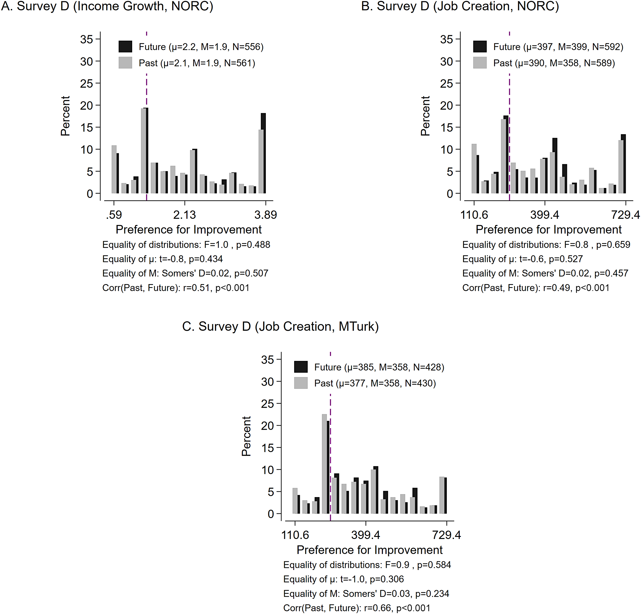
Figure 4. Long description
A three-panel figure labeled A, B, and C. Each panel contains a bar chart with Percent on the y-axis (0 to 35) and Preference for Improvement on the x-axis. A vertical dashed purple line marks the indifference point. Legends indicate black bars for Future and gray bars for Past.
* Panel A. Survey D (Income Growth, N O R C). X-axis ranges from .59 to 3.89. Future mean mu equals 2.2, median M equals 1.9, N equals 556. Past mean mu equals 2.1, median M equals 1.9, N equals 561. Statistical tests show F equals 1.0, p equals 0.488; t equals minus 0.8, p equals 0.434; Somers’ D equals 0.02, p equals 0.507; correlation r equals 0.51, p equals 0.000.
* Panel B. Survey D (Job Creation, N O R C). X-axis ranges from 110.6 to 729.4. Future mean mu equals 397, median M equals 399, N equals 592. Past mean mu equals 390, median M equals 358, N equals 589. Statistical tests show F equals 0.8, p equals 0.659; t equals minus 0.6, p equals 0.527; Somers’ D equals 0.02, p equals 0.457; correlation r equals 0.49, p equals 0.000.
* Panel C. Survey D (Job Creation, M Turk). X-axis ranges from 110.6 to 729.4. Future mean mu equals 385, median M equals 358, N equals 428. Past mean mu equals 377, median M equals 358, N equals 430. Statistical tests show F equals 0.9, p equals 0.584; t equals minus 1.0, p equals 0.306; Somers’ D equals 0.03, p equals 0.234; correlation r equals 0.66, p equals 0.000.
Results
Preference for improvement is attenuated, but not eliminated, when graph design discourages cognitive bias. The distributions in Figure 4A and 4C are left-shifted relative to their control group distributions in Figure 3. Median preference for improvement on income growth declines from 2.3% to 1.9% annual growth in Figure 4A (Past: t(1142) = −2.56, p = 0.01; Future: t(1131) = −2.68, p = 0.008). For job creation, only the MTurk sample yields a significant drop, from medians of 441,000 in the Future condition and 398,000 in the Past condition without debiasing, to 358,000 (regardless of time orientation) with debiasing (MTurk Past: t(831) = −4.28, p < 0.001; MTurk Future: t(831) = −3.72, p < 0.001; NORC Past: t(1175) = 0.41, p = 0.68; NORC Future: t(1171) = −0.71, p = 0.48).
After reducing bias in evaluating graphed trajectories, we continue to find support for the Universal Preference for Improvement Hypothesis. Mean and median indifference points remain substantially higher than the values in the fixed rising trajectory (dashed line), so the treatment reduces but does not eliminate preference for improvement. Distributions and central tendencies are statistically indistinguishable for Past and Future conditions in Figure 4. Preference for improvement looks like a genuine preference in evaluations of past and future aggregate conditions. In fact, for approximately one third of NORC respondents, preference for improvement is so strong that that they prefer an increasing sequence even when it is strictly dominated by a flat sequence. These respondents are willing to sacrifice higher ends and averages for an increasing trend. (The perfect collinearity of average, end point, and trend as we have defined them prevents us from independently quantifying the effect of each characteristic.)
We cannot rule out that other debiasing treatments would fully eliminate preference for improvement (and/or retrospective myopia and prospective hyperopia). Based on debiasing studies so far, however, people do indeed pay special attention to the final datapoints in a series and want trajectories to end on a high note—just not nearly by the margins that arise when plots show only sequences of per-period data.
DISCUSSION
People’s evaluations of aggregate conditions in the country, a key predictor of vote choice, respond predictably and powerfully to whether conditions are getting better. In many independent tests, we find a strong preference for improvement in both retrospection and prospection, supporting our Universal Preference for Improvement Hypothesis. People prefer improving to stagnant conditions even when conditions are initially quite poor and when the stagnant trajectory delivers greater welfare over the charted period. This finding holds when we discourage a heuristic assessment of graphs. An experimental treatment designed to downplay mindless reactions to trends attenuates preference for improvement but does not eliminate it, suggesting preference for improvement is at least in part a genuine preference rather than a cognitive bias. This preference appears to be nonpartisan: In Appendix H of the Supplementary Material, we test for partisan heterogeneity in myopia, hyperopia, and preference for improvement, with only one significant partisan interaction in over a dozen tests. In this section, we briefly discuss how our findings relate to vote choice and accountability, and how future research might build on them.
Preference for Improvement Outside the Survey Context
Our research occurred under controlled conditions: We observe myopia, hyperopia, and preference for improvement after asking participants to look at charts we created. We introduced noise into the charts to increase realism, but the charts used in the analyses are monotonic.Footnote 14 Doing so avoids potential confounds, as previous research finds sequence evaluations are swayed by violations of monotonicity in addition to ends, trends, and the total value of a sequence (e.g., Ariely and Carmon Reference Ariely and Carmon2000). In addition to overall improvement, a monotonic trend over four years may also convey consistency.Footnote 15 Our results are conditional on the degree of randomness and monotonicity in our stimulus materials. Future research might compare monotonic to nonmonotonic sequences with the same difference between start and end point. Such a design could clarify if people value improvement less when it is fitful and inconsistent.
At least two paths exist by which preference for improvement could affect electoral choice. First, voters might have a recollection of conditions in earlier periods, so they can assess changes in conditions when they see more recent statistics. Information about earlier periods might come from their own experiences or from previous exposure to statistical information. Given the public’s unimpressive levels of economic knowledge (e.g., Conover, Feldman, and Knight Reference Conover, Feldman and Knight1986; Prior and Lupia Reference Prior and Lupia2008), this path seems unlikely for evaluations of economic conditions. Healthcare premiums, local pollution, or traffic congestion might be more salient, but this path requires memory in addition to repeated information about conditions.
A second path involves voters encountering information similar to our experimental stimuli in the media. Anecdotally, examples abound of sequences of outcomes presented similarly to our treatments, including graphs of economic indicators (e.g., Zhang Reference Zhang2024) or projected economic growth (e.g., Stewart Reference Stewart2025). Media outlets show histories and projections in other domains (e.g., climate change; Plumer and Popovich Reference Plumer and Popovich2021). Systematic analyses of media reporting on the economy show routine coverage of change in past conditions and forecasts (Soroka, Stecula, and Wlezien Reference Soroka, Stecula and Wlezien2015; Stevenson and Duch Reference Stevenson and Duch2013). To the best of our knowledge, however, no research has thus far characterized the prevalence of histories and projections presented specifically as time-series graphs or the intervals over which media most typically report change in conditions.
People do seem to learn about conditions in the country, for example, the state of the economy, through exposure to media reporting (e.g., Duch, Palmer, and Anderson Reference Duch, Palmer and Anderson2000). Yet, without knowing if, how, and what people naturally learn about aggregate conditions, we cannot be sure that the evaluative strategies we observe in our study also occur outside the experimental context. Future research should study how voters experience and respond to trends of conditions in the country. It may leverage tools to track what content people see online (e.g., Guess Reference Guess2015) to understand whether they encounter graphical trends and if such exposure changes their opinions and vote choice.
Another research design would link improvement in actual or reported conditions—what, in the economic domain, Stevenson and Duch (Reference Stevenson and Duch2013) refer to as the “measured” and the “mediated” economy—to aggregated survey-based evaluations of conditions, such as the Index of Consumer Confidence (as in MacKuen, Erikson, and Stimson Reference MacKuen, Erikson and Stimson1992) or perceptions of the economy (as in Peress Reference Peress2024).
Attribution of Responsibility
We have left attribution of aggregate conditions and vote choice for future research. For example, our research designs deliberately stripped away political context, so we cannot say if the retrospective evaluations we measure relate to inferences about competence. In analyses that include the attribution of responsibility for retrospective conditions (such as Bartels Reference Bartels2008; Huber, Hill, and Lenz Reference Huber, Hill and Lenz2012), very low weights for the earliest datapoints might capture the judgment that an incumbent should not be held accountable for conditions early in her term over which she might have had little control. (This logic does not apply to evaluations of conditions in our design, however: the question we ask is not about apportioning credit, only about assessing the depicted conditions.) While attribution might introduce partisanship into people’s evaluations (Bisgaard Reference Bisgaard2015), preference for improvement is equally pronounced among Democrats and Republicans.
Evaluations of aggregate conditions play a central role in models of vote choice. Our research design does not speak to the effect of preference for improvement or retrospective myopia on how people vote. It is for future research to investigate if the prospective hyperopia or preference for improvement affects assessments of candidates (via judgment about competence or something closer to issue voting). With a straightforward extension, the current design can be used to examine effects of conditions on attribution and vote choice. A between-subject design could present different subsets of respondents with different conditions, then elicit vote intention (see, e.g., Andrews and Bokemper Reference Andrews and Bokemper2025; Huber, Hill, and Lenz Reference Huber, Hill and Lenz2012 for incentivized settings). Collaborations with officeholders could randomize information about conditions, such as the length of the history shown or the number of intervals in a trajectory.
Implications for Accountability and Candidate Strategy
Our results speak to candidate strategy. If presentation of data about aggregate conditions can alter the evaluations people form, then candidates for office can do what we did: show data that invite biases or try to discourage these biases. This gives candidates two routes to gain support: they can produce or propose improvement of conditions that people notice and select, or they can create the appearance of such improvement, for example, by showing charts with increasing trends in favorable conditions.
During election campaigns, past conditions set a baseline for strategic candidates, reminiscent of Vavreck’s (Reference Vavreck2009) model, where election forecasts based on economic data determine which candidate is favored to win the election if the campaign focuses on the economy. In her model, the underdog according to the forecast needs to disrupt the campaign’s focus on the economy. In our application, the trajectory of past economic conditions similarly determines which candidate is favored if conditions are displayed by trend charts. The candidate hurt by potential trend interpretation of economic data would then aim to counteract the focus on improvement in conditions by using other graphical formats (e.g., highlighting average or cumulative performance rather than change) or not using graphs at all.
The same logic extends to how candidates or media outlets choose to present information about policies and their projected impacts. Candidates, for example, might emphasize the trajectory of a policy that is costly now but has the potential to deliver benefits in the future (e.g., in discussing climate change mitigation policies). When discussing policies with immediate benefits and longer-term costs (e.g., underfunded tax cuts), they may do the opposite. Future work should consider how candidates and other political actors strategically anticipate preference for improvement, adjusting their presentation of data or emphasis on certain timeframes to avoid presentations that show conditions under their control worsening over time.
To understand how much preference for improvement guides electoral choice, researchers need to know not only how often voters see the “mediated economy” (Stevenson and Duch Reference Stevenson and Duch2013) in charts but also what the motivations are of the chart-makers. When preference for improvement favors their side, strategic actors will depict conditions in charts as much as they can. The disadvantaged side will not, but they cannot undo their opponents’ charts.
CONCLUSION
This study contributes to understanding evaluations of aggregate conditions, the first step in a process that may ultimately produce political accountability. Downweighting of past outcomes earlier in an election cycle is detrimental from some theoretical perspectives, particularly purely retrospective sanctioning models in which voters look at past performance only to punish or reward incumbents (Ferejohn Reference Ferejohn1986; Gieczewski and Li Reference Gieczewski and Li2024; Key Reference Key1966; Kramer Reference Kramer1971). Disproportionate weighting of recent conditions amounts to an incomplete assessment of evidence regarding the incumbent’s performance—myopia impedes accountability (e.g., Healy and Lenz Reference Healy and Lenz2014). From this perspective, “it seems likely that public welfare would be enhanced if voters took a longer view with respect to the economy” (Healy and Malhotra Reference Healy and Malhotra2013, 199).
In selection models of electoral choice, people also draw on past performance evaluations but do so in order to determine the competence of the incumbent (Alesina, Londregan, and Rosenthal Reference Alesina, Londregan and Rosenthal1993; Fearon Reference Fearon, Przeworski, Manin and Stokes1999; Persson and Tabellini Reference Persson and Tabellini1994). In such a model, the empirical pattern of retrospective “myopia” may lead to the selection of “good types” with the capacity for generating improvement in conditions in the future. The very same empirical pattern, retrospective myopia, that is detrimental in a sanctioning model, might reflect future-oriented considerations to optimize performance.
The empirical pattern in our Past treatment thus has ambiguous theoretical implications. The Future treatment offers tentative separation of the two theories. It shows that people look for improvement, not the quickest benefit. This preference is an individual characteristic: the more people prefer improvement in the past, the stronger their preference for future improvement. The combined results for Past and Future cannot rule out that people overweight the recent past because they are short-sighted specifically when looking back, but they offer preference for improvement as a general and more parsimonious psychological underpinning.
The juxtaposition of myopic retrospection and preference for improvement raises interesting questions about the different blind spots. When retrospective evaluations are myopic, recent conditions receive similar overall evaluations regardless of how things were earlier on in the time series. Relying on the end heuristic specifically, early conditions are neglected as voters inadvertently substitute their perception of the most recent conditions for the conditions during the entire series (e.g., Healy and Lenz Reference Healy and Lenz2014; Kahneman et al. Reference Kahneman, Fredrickson, Schreiber and Redelmeier1993). All else being equal, myopic people are indifferent between exceptionally good early conditions and abysmally poor early conditions—they respond only to the most recent conditions. Retrospectively myopic individuals will sometimes leave good (early) conditions unrewarded and sometimes leave poor (early) conditions unpunished.
In contrast to myopic individuals, people drawn to improving conditions take into account the early datapoints in a series in order to assess change over time. While it is difficult to distinguish cleanly between myopia and preference for improvement in retrospection (see Prior, Alsharawy, and Andrews Reference Prior, Alsharawy and Andrews2023 for evidence for retrospective myopia using a different measurement approach), our findings for prospection are clear: people give most weight to the most distant outcomes and again value improvement. The shorthand of the “myopic voter” is unhelpful because voters do not behave in this fashion when assessing future conditions. We emphatically reject the Universal Myopia Hypothesis.
These more holistic evaluations of the entire sequence are not without pitfalls, however. Individuals governed by preference for improvement will punish good conditions when they are followed by worse conditions and reward poor conditions when they are followed by better conditions. Preference for improvement may thus lead individuals to accept greater overall welfare loss than myopia. This has the potential to distort accountability more than retrospective myopia does because myopia only neglects early conditions, whereas preference for improvement rewards a low starting point. Although participants in our research were not entirely unresponsive to the total benefit provided by the charted conditions, they consistently traded off some of that welfare for greater improvement over time.
Even if there is potential rationality in selecting competent candidates by focusing on improvement, this does not mean people are particularly good at doing so. Preference for improvement is very strong in our studies, and only partly an impulse we can suppress by displaying data differently. Many people prefer improving conditions at substantial cost of overall welfare. Many continue to do so when we point out that cost. And they continue to do so when we tell them that continued improvement is no more likely than returning to the poor starting point. There is hardly redemption in a public not being short-sighted but instead choosing improvement when alternative scenarios are clearly superior. Chasing improvement may have a more optimistic ring to it than myopia, but it, too, can be self-defeating.
SUPPLEMENTARY MATERIAL
To view supplementary material for this article, please visit http://doi.org/10.1017/S0003055426101853.
DATA AVAILABILITY STATEMENT
Research documentation and data that support the findings of this study are openly available at the American Political Science Review Dataverse: https://doi.org/10.7910/DVN/SHQKBM.
ACKNOWLEDGMENTS
For comments and advice on earlier versions, we thank Abdelaziz Alsharawy, Scott Althaus, Alan van Beek, John Bullock, Charlotte Cavaille, Andy Delton, Brian Guay, Shigeo Hirano, Josh Kalla, Yph Lelkes, Yotam Margalit, John Marshall, Tali Mendelberg, Michael Peress, Eric Schickler, Kodiak Sauer, Florian Sichart, Randy Stevenson, Laura Stoker, David Villacis-Calderon, audiences at UC Berkeley, Princeton, and the Rebecca B. Morton Conference on Experimental Political Science at NYU, and in particular Gabe Lenz. Justin Curl provided programming assistance.
FUNDING STATEMENT
This research was supported in part by a grant from the Data-Driven Social Science Initiative at Princeton University and research time made possible by a fellowship from the Andrew Carnegie Foundation.
CONFLICT OF INTEREST
The authors declare no ethical issues or conflicts of interest in this research.
ETHICAL STANDARDS
The authors declare the human subject research in this article was reviewed and approved by Princeton University’s IRB. The authors affirm that this article adheres to the principles concerning research with human participants laid out in APSA’s Principles and Guidance on Human Subject Research (2020).
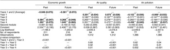
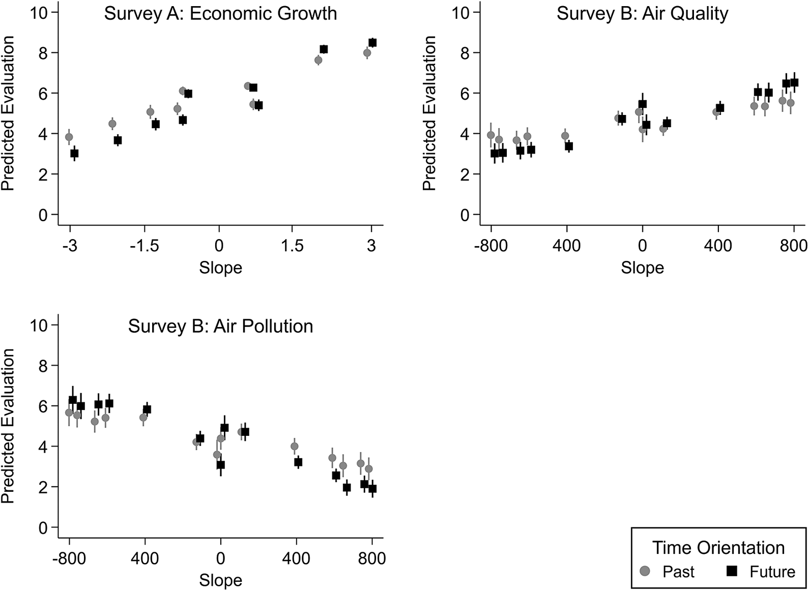
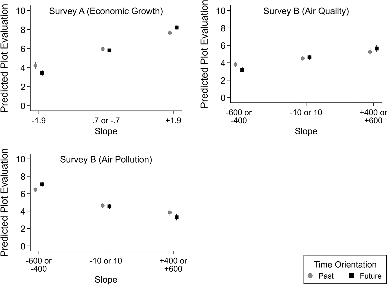
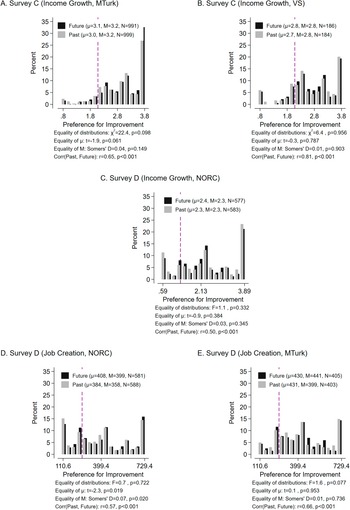
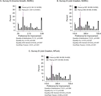


 Open access


Comments
No Comments have been published for this article.