I. INTRODUCTION
The problem of determining intrinsic film properties from indentation data that are influenced by both film and substrate is an old one. If the film is thick enough to be treated as a bulk material, then the analysis of Oliver and PharrReference Oliver and Pharr1 is typically used. Doerner and Nix were the first to propose a model for extracting the film modulus from substrate-affected modulus. Their model assumed a linear transition from film to substrate, and it included a constant that had to be determined empirically.Reference Doerner and Nix2 KingReference King3 improved upon the Doerner–Nix model by using integral equation analysis to achieve a form with no adjustable parameters. Shield and Bogy derived a model from a rigorous analysis of a punch pressing into a layered elastic half space. This model was physically unsatisfying, however, as it predicted discontinuous contact along the punch face.Reference Shield and Bogy4
Gao et al., drawing from the work of previous investigators, proposed a simple approximate model with no adjustable parameters. They derived two functions, I 0 and I 1, to govern the transition in elastic properties from film to substrate.Reference Gao, Chiu and Lee5 These functions have been retained and variously used by others. Menčík et al. proposed several practical refinements to the implementation of the Gao model, including a correction to the film-thickness term to account for surface penetration when using a Berkovich indenter.Reference Menčík, Munz, Quandt, Weppelmann and Swain6 This correction proposed by Menčík has been adopted by others using or improving upon the Gao model. Song and colleagues took an alternate solution path, which was originally suggested by Gao et al. but not followed. This path yielded a simpler form that predicts the composite response better if the film is more compliant than the substrate.Reference Song7–Reference Xu and Pharr9 This model is called the “Song–Pharr model” in the literature. Independently, Bec et al. proposed another simple closed-form model.Reference Bec, Tonck, Georges, Georges and Loubet10, Reference Roche, Bec, Loubet, Bahr, Kung, Moody and Wahl11 Of these models, the Bec model and the Song–Pharr model work reasonably well for compliant films on stiff substrates; the Bec model slightly overpredicts the influence of the substrate, whereas the Song–Pharr model slightly underpredicts the same.Reference Hay12 However, none of the models covered in this review accurately predicts response if the film modulus is more than twice the substrate modulus. This shortcoming motivated this work.
Since its inception, finite-element analysis (FEA) has been essential to the development and verification of analytic contact models. Nearly, all the aforementioned thin-film models were evaluated and refined by means of FEA because FEA idealizes experiment. In a finite-element model, the film thickness, film properties, and substrate properties are all well known because they are required inputs. Also, there is little ambiguity about the true contact area under load because it is determined from the last node(s) in contact. So, before turning to experimentation, the worth of an analytic model is first assessed by means of FEA. For example, an elastic finite-element model may be constructed with a film of thickness t on a substrate, with the input properties of film and substrate being E f, ν f, E s, and ν s. Then, indentation into the material is simulated, and the simulated force–displacement data are analyzed to achieve a value for the Young’s modulus of the film, i.e., E f-out. What is the difference between this output value and the value that was used as an input to the finite-element model? FEA allows this question to be answered systematically over the domain of situations that might be encountered experimentally: thick films, thin films, stiff films on compliant substrates, compliant films on stiff substrates, etc. If an analytic model applied to simulated data fails to return the input properties with sufficient accuracy, it should not be expected to work well when applied to experimental data.
Indentation into a film–substrate system generally does not produce a contact of the same shape as would be achieved in a semi-infinite body having the same properties as the film.Reference Saha and Nix13 Thus, the analysis of Oliver and PharrReference Oliver and Pharr1 for predicting contact area may not yield a sufficiently accurate measure of the true contact area. When the film is more compliant than the substrate, the tendency is for the film material to “pile-up” around the face of the indenter, meaning that the Oliver–Pharr analysis will underpredict the true contact area.Reference Saha and Nix13 If the film is stiffer than the substrate, the tendency is for the film to be pressed into the substrate well outside the contact area, meaning that the Oliver–Pharr analysis will overpredict the true contact area.Reference Ni and Cheng14 These phenomena are evident in FEA, but they do not present a problem because the contact area can be obtained from the mesh. But these phenomena can present a practical problem for the experimenter. Finite-element simulations can be used to identify experimental conditions under which such problems may arise.
In this work, a new analytic model is presented that is informed by and improves upon previous analytic models. The new model is tested and refined by FEA over the domain 0.1 < E f/E s < 10 and 4% < h/t < 40%. The simulations are also used to identify the conditions under which the Oliver–Pharr analysis for determining contact error should be expected to work well. Finally, the analytic model is assessed experimentally by instrumented indentation testing of both stiff and compliant films.
II. THEORY
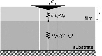
The present model is a development of the Song–Pharr model, which in turn draws from the Gao model. The Song–Pharr model is illustrated schematically in Fig. 1. It assumes that a column of material under the indenter, defined by the contact radius, can be isolated from the surrounding material and treated as two springs in series, with the influence of each spring weighted according to a/t through the function I 0. The measured (or apparent) shear modulus (μ a) is related to the shear modulus of the film (μ f) and that of the substrate (μ s) through this expression:

Schematic of the Song–Pharr model, which assumes that material under the indenter can be isolated from surrounding material and treated as springs in series. The constant D = 4a/(1 – ν a) relates bulk modulus to stiffness; it cancels out of the expression derived from this model [Eq. (1)].

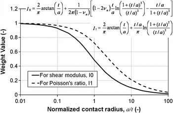
The weighting function, I 0, is that of Gao et al.Reference Gao, Chiu and Lee5 It provides a smooth transition from film to substrate. When I 0 is unity, as it is when the contact radius is small relative to the film thickness, then μ a = μ f. As the penetration increases, the value of I 0 approaches zero, which makes μ a = μ s. The function I 0 is plotted in Fig. 2 and given by

Gao’s weighting functions I 0 and I 1, which govern the film-to-substrate transition for shear modulus and Poisson’s ratio, respectively.

The Song–Pharr approach is valuable because it includes a clever simplification, which separates the effect of transition in bulk modulus from the relatively minor effect of transition in Poisson’s ratio. The simplified form of Eq. (1) is achieved by assuming that a single apparent Poisson’s ratio, ν a, can be used to represent the behavior of the entire column of the material. The expression for this apparent value isReference Song7

In this expression for ν a, the weighting function, I 1, is also due to Gao. It is plotted in Fig. 2 and given by

When I 1 is unity, as it is when the contact radius is small relative to the film thickness, then ν a = ν f. As the penetration increases, the value of I 1 approaches zero, which makes ν a = ν s. If film and substrate have the same Poisson’s ratio (that is, if ν s = ν f = ν), then Eq. (3) reduces to ν a = ν for all values of I 1.
Ultimately, we shall modify the form of Eq. (1) to better model stiff films on compliant substrates. However, we shall retain the weighting functions of Gao and the separation and definition of Poisson’s ratio suggested by Song and Pharr. That is, the expressions of Eqs. (2)–(4) are used in the new model without modification. Further, we shall follow Menčík’s suggestion that when using a Berkovich indenter, the film thickness t used in Gao’s weight functions should be the original film thickness, t 0, less the contact depth: t = t 0 – h c.
We must modify the form of Eq. (1) because high-stiffness films pose a problem for the Song–Pharr model.Reference Xu and Pharr9 As the film modulus becomes large, the apparent compliance (1/μ a) should go to zero, but Eq. (1) does not predict this. Rather, it predicts that the apparent compliance will be governed by the compliance of the substrate, meaning that the apparent compliance calculated by Eq. (1) will be too large. The root cause of the problem is that the material under the indenter cannot be isolated from the surrounding material, because the film offers significant lateral support. The behavior is like that of a drum: upon being struck, the response is governed primarily by the drum skin—its elastic properties, thickness, and boundaries—not by the near-zero compliance of the air underneath the drum skin.
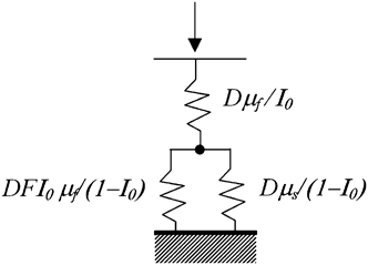
To improve upon the Song–Pharr model, we suppose that phenomenologically, the film can also act as a spring in parallel with the substrate as illustrated schematically in Fig. 3. There are several ways to consider the sense of this configuration. First, as the film becomes stiff, it dominates the response, and this is what happens with parallel springs—the stiffer spring dominates. Second, as the film becomes thin and stiff, the deformation in the top layer of the substrate approaches that of the film. If two springs of different stiffness experience the same deformation subject to the same force, then they should be modeled as parallel. Finally, if the film provides significant lateral support, then it effectively acts on the indenter like the leaf springs that support the indenter column, and these leaf springs are well modeled by a parallel spring.Reference Oliver and Pharr1
Schematic of the proposed model allowing the film to act in series and in parallel with the substrate. The constant D = 4a/(1 – ν a) relates bulk modulus to stiffness; it cancels out of the expression derived from this model [Eq. (5)].

Springs in parallel are treated together by adding their stiffnesses. Thus, the proposed model is

In the denominator of the first term on the right-hand side, the influence of the film modulus is moderated by two factors: I 0 and F. The moderation with I 0 makes the film influence degrade with depth. We also allow for moderation with the tunable constant, F, because we do not know, a priori, the importance of film modulus relative to that of the substrate. We shall determine the best value for the constant F using FEA.
Equation (5) gives us the right behavior in the limits of I 0 → 1, I 0 → 0, μ f << μ s, and μ f >> μ s. When I 0 is close to 1, as it is at shallow penetration depths, the apparent modulus approaches that of the film. As I 0 approaches 0, as it does at large depths, the apparent modulus approaches the substrate modulus. In the case of a compliant film on a rigid substrate (μ f << μ s), Eq. (5) reduces to the Song–Pharr model [Eq. (1)] for all values of I 0. Finally, when the film modulus is very large, the apparent compliance goes to zero for all values of I 0, as it should.
Thus, the shear modulus of the film is calculated from the apparent value by solving Eq. (5) for μ f:

where A = FI 0


Finally, the Young’s modulus of the film is calculated from the shear modulus and Poisson’s ratio as

The remainder of this article comprises the validation of Eqs. (5)–(7) by simulation and experiment. It should be noted that the application of Eqs. (5)–(7) presumes that the apparent shear modulus, μ a, has already been calculated. The means for doing so have been well documented elsewhere,Reference Oliver and Pharr1, Reference Hay15–Reference Oliver and Pharr17 but a summary of the process is provided here in the Appendix.
III. FINITE-ELEMENT ANALYSIS
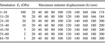
Seventy axisymmetric finite-element simulations were performed using Cosmos 2.8. These simulations are summarized in Table I. An updated Lagrangian formulation was used to handle potentially large strains. The solution was achieved in discrete time steps. At each time step, the solution was found by force control with Newton–Raphson iteration.
Summary of finite-element simulations, showing values for inputs that were varied.

For all simulations, the indenter was a 2-dimensional version of a Berkovich diamond. For the sample, t = 500 nm, E f = 10 GPa, and ν f = ν s = 0.25.
Some simulation inputs were fixed and some were systematically varied to investigate the domain of interest. The film thickness was set to 500 nm for all simulations; indentation depth was varied to investigate the domain of 4% < h/t < 40%. All indented materials, both film and substrate, were assigned a Poisson’s ratio (ν) of 0.25 and a linear elastic stress–strain curve. (Thus, neither the effect of plasticity nor that of transition in Poisson’s ratio was investigated by FEA.) The Young’s modulus of the film was fixed at 10 GPa. To achieve the desired variation in E f/E s, the substrate modulus varied between 100 GPa (E f/E s = 0.1) and 1 GPa (E f/E s = 10). Because Poisson’s ratio was set to 0.25 for all materials; the modulus ratios are the same whether expressed in terms of Young’s modulus or shear modulus, i.e., μ f/μ s = E f/E s.
The purpose of simulations 31–40 was to verify the finite-element model. For these simulations, the finite-element model had the mesh of a film–substrate system, but with film and substrate having the same modulus (i.e., E f = E s =10 GPa) and so behaving as a bulk sample. Thus, the intention was to verify the general finite-element model by showing that for simulations 31–40, standard analysis of simulated data yields an output modulus that is very close to the input value.
For all simulations, the indenter was a cone having an included angle of 140.6° and an apical radius of 50 nm. This shape is the two-dimensional analog of the common Berkovich indenter. The indenter was defined to be a linear elastic material having the properties of diamond: E = 1140 GPa and ν i = 0.07.
Both the indenter and the sample were meshed with four-node axisymmetric plane strain elements. For the sample, the extent of the mesh was 90a′ in both the radial and axial directions, where a′, the anticipated contact radius, was calculated as the radius of the indenter at a distance from the apex that is equal to the specified indentation depth. The radial extent of the fine mesh near the contact was 1.2a′. The resolution of the fine mesh was set so that at least 35 material nodes were in contact with the indenter at the maximum penetration. The radial extent of the indenter mesh was 45a′, and the axial extent was 90a′.
The boundary conditions were specified as follows. Along the right-hand side and bottom of the sample, all nodes were rigidly fixed. Along the axis of symmetry, nodes were constrained to move along the axis of symmetry only (ux = 0). Nodes along the top of the indenter were displaced downward by the total prescribed displacement that took place in discrete time steps. Nodes along the right-hand side of the indenter were unconstrained. The interaction between the indenter and the sample was handled as follows: the nodes along the indenter form a curve, surface nodes on the sample were not allowed to pass to the other side of this curve (line-contact formulation), and no slip was allowed between film and substrate.
The contact area as determined from the finite-element mesh was taken to be the “true value” and the basis for evaluating the contact area as determined by the Oliver–Pharr analysis. The method for determining the contact radius from the finite-element mesh was more sophisticated than simply taking the radial position of the last node in contact. The contact radius was determined as the radial position of the intersection of two lines: one defined by the last two nodes in contact (radially) and one defined by the first two nodes out of contact (radially). This method provided a smooth increase in contact radius, as opposed to discrete increments with each new contact node.
IV. EXPERIMENTAL METHOD
Seventeen samples were tested in this work to examine a range of film thickness and modulus mismatch. For the first 14 samples, the film was more compliant than the substrate; these samples are described further in next section. For the last three samples, the film was stiffer than the substrate; these samples are described further in Sec. IV. B.
A. Compliant films on stiff substrates
All samples in this category were provided by SEMATECH (Austin, TX), a consortium representing companies in the semiconductor industry. Three sets of silicon wafers coated with dielectric materials were evaluated. For the Young’s modulus of the substrate, a value of 170 GPa was used for all samples in this category. All films were deposited by chemical vapor deposition (CVD). Each set had four or five wafers of nominally the same film deposited in different thicknesses (200–2000 nm). Wafer set 1 comprised five wafers of silane oxide films (κ ∼ 4.0). Wafer set 2 comprised five wafers of non-porous “low-κ” films (κ ∼ 2.9); the composition of this dielectric material was confidential. Wafer set 3 comprised four porous “ultra-low-κ” films (κ ∼ 2.3). The composition of this dielectric material was also confidential. The films in wafer set 3 were deposited with a “porogen” and then exposed to an ultraviolet (UV) cure process to cause residual pores. Cure times varied with film thickness, with thicker films exposed to longer cures; however, the SEMATECH representative who made the samples doubted that the UV could penetrate beyond 1000 nm into the surface.
B. Stiff films on compliant substrates
Three samples in this category were evaluated. The first sample (15) was a 2600 nm chromium nitride (CrN) coating deposited on a cold-work tool steel that had been polished to a surface roughness of 20 nm (R a). The coating was deposited in an industrial PVD system METAPLAS Ionon MZR 323 (Sulzer Metaplas GmbH, Bergisch-Gladbach, Germany) equipped with 6 Cr (99.5% purity) planar cathodic arc sources. For this sample, a value of 230 GPa was used for the substrate Young’s modulus. The last two samples (16 and 17) were 150 and 300 nm silicon nitride (SiN) coatings on silicon wafers. The SiC films were deposited onto prime silicon substrates using an industrial PVD system equipped with a planar magnetron sputter source and 99.99% pure silicon carbide target. For these samples, a value of 170 GPa was used for the substrate Young’s modulus.
C. Testing equipment and method
Physical indentation experiments on these 17 samples were performed using Agilent nano-indentation systems. Only diamond Berkovich indenter tips were used. At least 10 tests were performed on each sample. All tests used the continuous-stiffness measurement option, which oscillates the indenter to return contact stiffness as a continuous function of penetration depth.Reference Oliver and Pharr1 The CrN-on-steel sample was tested with an XP actuator–transducer; all other samples were tested with a DCM actuator–transducer. Test method and analysis were standard and have been described in detail elsewhere.Reference Oliver and Pharr1, Reference Hay, Agee and Herbert16, Reference Pharr, Strader and Oliver17
V. RESULTS
A. Finite-element results
We can have confidence in the finite-element results because application of standard analysis to the simulated data from runs 31–40 (for which E f/E s = 1) yields an output modulus that differs from the input value by no more than 1%. This close agreement is achieved by using contact area as calculated from the finite-element mesh, not as calculated by the Oliver–Pharr method.
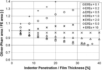
One aspect of “substrate effect” is the extent to which the substrate affects the ability to determine contact area by the Oliver–Pharr method.Reference Oliver and Pharr1 Figure 4 shows the Oliver–Pharr contact area relative to the finite-element area for all simulations. Values less than unity indicate pile-up, and values greater than unity indicate excessive sink-in. For simulations 31–40, the Oliver–Pharr method yields a contact area that is within 3% of the finite-element area; this agreement is excellent, given the simplicity of the calculation.
Evaluation of the ability to calculate contact area by the Oliver–Pharr method as a function of film/substrate mismatch and indentation depth. For E f/E s = 1, the Oliver–Pharr method gives a contact area that is within 3% of the finite-element value.

The error in the contact area achieved by the Oliver–Pharr method depends on whether the film or substrate is more compliant, the degree of modulus mismatch, and the indentation depth relative to the film thickness. The compliant films on stiff substrates exhibit a tendency to pile-up, meaning that the areas calculated from the Oliver–Pharr method are too small, with the severity of the problem increasing with the degree of modulus mismatch and indentation depth. The stiff films on compliant substrates exhibit a tendency to sink-in excessively, meaning that the areas calculated from the Oliver–Pharr method are too large. Again, the error magnitude increases with the degree of modulus mismatch and indentation depth. However, for the same degree of mismatch and relative indentation depth, the error for stiff films is much greater than that for compliant films.
Figure 4 allows us to predict the error in modulus due to shortcomings in the Oliver–Pharr method for determining contact area. The corresponding error in modulus is half the magnitude of the error in contact area and of the opposite direction because the calculation for modulus from indentation data depends inversely on the square root of the contact area (1/√A). For example, if the calculated contact area is 10% larger than the true contact area, the resulting value of modulus will be 5% smaller than the true modulus. For compliant films (0.1 ≤ E f/E s < 1), the error in modulus should be less than about 5% if the indentation depth is less than 10% of the film thickness. For moderately stiff films (1 < E f/E s ≤ 2), the error in modulus should be less than 5% so long as the indentation depth is less than 20% of the film thickness. For very stiff films (E f/E s > 2), the error due to the area calculation is substantial at all practical indentation depths. For such samples, the Oliver–Pharr method for determining contact area should not be used.
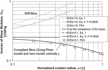
Another aspect of “substrate effect” is the composite response of the film and substrate to the indentation force. Figure 5 shows the inverse of the apparent shear modulus (hereafter apparent compliance) as a function of normalized contact radius for film/substrate systems having the most severe modulus mismatch (E f/E s = 0.1 and E f/E s = 10). The centerline marks the true value for the film—that is, the finite-element input value. Results for stiff films on compliant substrates are plotted in gray above this centerline; results for compliant films on stiff substrates are plotted below. The open symbols are the values obtained from the finite-element simulations. Each plotted point represents a single simulation of pressing the indenter into the film to a prescribed depth and withdrawing it, then analyzing the simulated force–displacement data in the usual way, but using contact area as calculated from the finite-element mesh. The dashed curves show the apparent compliance as predicted by the Song–Pharr model [Eq. (1)], given the film thickness, material properties, and contact geometry. The solid curves show the apparent compliance as predicted by the new model [Eq. (5)], given the same information and a single value for the empirical constant of F = 0.0626. (The means by which F was determined are explained subsequently.) For compliant films on stiff substrates, the Song–Pharr model and the new model are indistinguishable; they predict the finite-element results equally well. But for stiff films on compliant substrates, the new model provides a much better prediction of finite-element results. Rar et al. published a nearly identical plot comparing their own finite-element simulations (via ABAQUS) to the Song–Pharr model.Reference Rar, Song, Pharr, Ozkan, Freund, Cammarata and Gao8
Comparison between two models and finite-element results for the film/substrate systems having the most severe modulus mismatch. For compliant films, the Song–Pharr model and the new model are the same; for stiff films, the new model is substantially better than the Song–Pharr model at predicting apparent compliance.

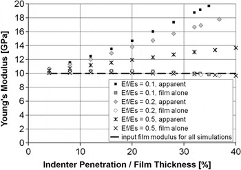
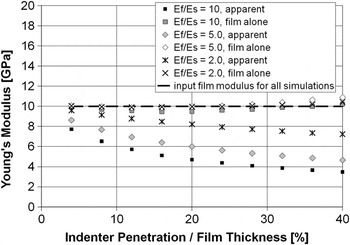
The new model expressed by Eq. (5) allows us to compute the Young’s modulus of the film by using Eqs. (6)–(7) with F = 0.0626. Figure 6 shows Young’s modulus versus normalized penetration for the 30 simulations of indentation into compliant films on stiff substrates (simulations 1–30). All values have been computed using contact area as determined by the finite-element mesh. The dark symbols represent the substrate-affected modulus that would be obtained by standard analysis. The light symbols represent the film modulus as computed by Eq. (7). The values for film modulus determined in this way agree well with the FEA input value of 10 GPa, even for penetration depths as large as 40% of the film thickness. Figure 7 shows analogous results for the 30 simulations of indentation into stiff films on compliant substrates (simulations 41–70). Within the domain of h/t < 25%, the proposed model never over-corrects. Within the domain of 25% < h/t < 40%, the model over-corrects slightly.


A single value for the empirical constant F was determined as the value that minimized the sum of the squared differences between the input Young’s modulus for the film (10 GPa) and the output value as computed by Eq. (7) across all 70 finite-element simulations. Variances were not weighted. The value for the empirical constant determined in this way was F = 0.0626. This single value for F was used in the analysis of all simulated and experimental results.
B. Experimental results
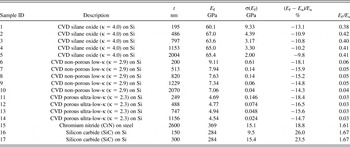
All experimental results are summarized in Table II. For all samples, values for modulus (E f and E a in Figs. 8–13) were computed using the Oliver–Pharr contact area. The consequential error in modulus should be less than 5% as explained in Sec. V. A.

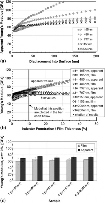
Analytical sequence for the first wafer set (samples 1–5) showing (a) apparent (substrate-affected) modulus as a function of indenter penetration, (b) apparent modulus and film modulus as a function of normalized indenter penetration, and (c) values at 10% of film thickness. In (a) and (b), the trace for each sample represents the average of all tests on that sample. For clarity, error bars spanning one standard deviation are shown only on the bar chart (c).

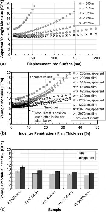
Analytical sequence for the second wafer set (samples 6–10) showing (a) apparent (substrate-affected) modulus as a function of indenter penetration, (b) apparent modulus and film modulus as a function of normalized indenter penetration, and (c) values at 10% of film thickness. In (a) and (b), the trace for each sample represents the average of all tests on that sample. For clarity, error bars spanning one standard deviation are shown only on the bar chart (c).

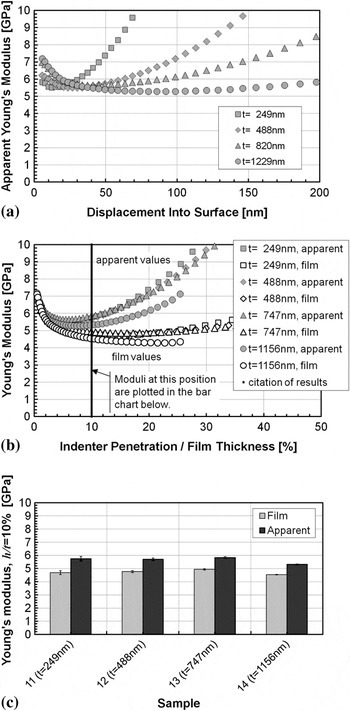
Analytical sequence for the third wafer set (samples 11–14) showing (a) apparent (substrate-affected) modulus as a function of indenter penetration, (b) apparent modulus and film modulus as a function of normalized indenter penetration, and (c) values at 10% of film thickness. In (a) and (b), the trace for each sample represents the average of all tests on that sample. For clarity, error bars spanning one standard deviation are shown only on the bar chart (c).

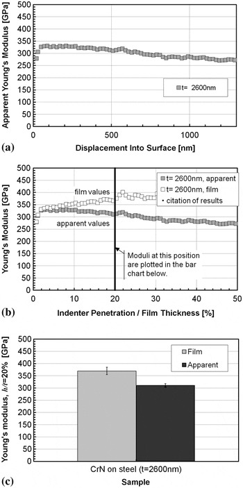
Analytical sequence for the single sample of CrN on steel showing (a) apparent (substrate-affected) modulus as a function of indenter penetration, (b) apparent modulus and film modulus as a function of normalized indenter penetration, and (c) values at 20% of film thickness. In (a) and (b), the trace for each sample represents the average of all tests on that sample. For clarity, error bars spanning one standard deviation are shown only on the bar chart (c).

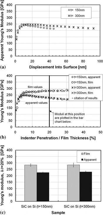
Analytical sequence for the two samples of SiC on Si showing (a) apparent (substrate-affected) modulus as a function of indenter penetration, (b) apparent modulus and film modulus as a function of normalized indenter penetration, and (c) values at 20% of film thickness. In (a) and (b), the trace for each sample represents the average of all tests on that sample. For clarity, error bars spanning one standard deviation are shown only on the bar chart (c).

Summary of experimental results.

For sample 15, the substrate Young’s modulus (E s) was assumed to be 230 GPa; for all other samples, the substrate Young’s modulus was assumed to be 170 GPa.
1. Compliant films on stiff substrates
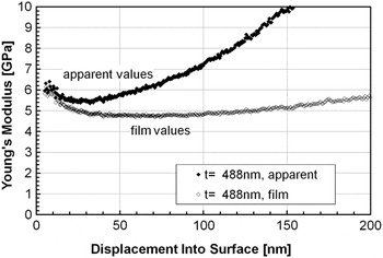
Figure 8 shows both apparent modulus and film modulus for one test on sample 12—an ultra-low-κ film (488 nm) on silicon. These two traces represent different analyses of identical physical measurements. The apparent modulus (black symbols) is obtained by standard analysis, and the film modulus (gray symbols) is obtained by Eqs. (5)–(7). At small displacements, the two traces coincide; they gradually diverge with displacement. With displacement, the apparent modulus manifests the increasing influence of the silicon substrate, whereas the film modulus decreases to a constant value (about 4.8 GPa), which persists out to about 100 nm (∼20% of the film thickness).
For both traces shown in Fig. 8, the contact area is determined by the Oliver–Pharr method. For compliant films on stiff substrates, FEA shows that the Oliver–Pharr method yields values for contact area that are smaller than the true values owing to pile-up, with the severity of the problem increasing with indentation depth. Recalling that an error that makes contact area too small has the effect of making the modulus calculated from that area too large, we conclude that the increase in film modulus seen in Fig. 8 at depths greater than 100 nm is due more to an errant measure of contact area than to inadequacies in the model correcting for substrate influence.
Figure 9 shows the progression of analysis for the five oxide films on silicon (samples 1–5). Figure 9(a) shows the apparent Young’s modulus achieved by standard analysis as a function of indentation depth. The trace for each sample represents an average of all tests on that sample. Figure 9(b) shows both the apparent modulus and the film modulus plotted as a function of relative indentation depth. Plotting the data in this way reveals the similarity of the five samples; substrate influence merely depends on relative indentation depth. The film modulus calculated according to Eqs. (5)–(7) is constant out to more than 30% of the film thickness. Finally, Fig. 9(c) shows moduli measured at 10% of the film thickness, with error bars spanning one standard deviation. [For clarity, error bars were omitted from Figs. 9(a) and 9(b).] Within the uncertainty of the measurement, all five samples have the same film modulus, which is about 10% lower than the apparent modulus.
Figure 10 shows the same analytic progression as Fig. 9 for the five “low-κ” films on silicon (samples 6–10). For these samples, the film modulus at 10% of the film thickness is about 15% lower than the apparent modulus at the same position. Among these samples, the film modulus decreases slightly, but significantly, with film thickness. There is something about the microstructure of this film material that causes Young’s modulus to change with film thickness. Thus, for this material, it is important to be able to measure properties on a sample that is of the same thickness as what will actually be used in product. Making a thicker version of the same material to measure substrate-independent modulus is not an option.
Figure 11 shows the same analytic progression for the four “ultra-low-κ” films on silicon (samples 11–14). Figure 11(b) shows a significant elevation in modulus at the surface. Accounting for the substrate-influence makes this difference at the surface more obvious. This difference may be a consequence of high UV exposure or of a closed-pore surface. Figure 11(b) also reveals that the modulus of the thickest sample (14, t f = 1156 nm) is significantly lower than that for the other three thinner samples. This was expected because the UV does not cure materials deeper than 1000 nm into the surface. This interlayer of uncured material effectively acts as a compliant substrate and thus increases the sensed compliance even when the indenter is well within the cured material. Within the uncertainty of the measurement, the three thinnest samples in this set (samples 11–13) all have the same film modulus, which is about 17% lower than the apparent modulus.
For samples 11–14 (Fig. 11), there may be a third mechanism for the increase in apparent modulus with indenter displacement. These samples are porous and may densify as a consequence of indentation, which would cause the material to become stiffer. No accounting of this effect has been made in this work.
2. Stiff films on compliant substrates
Figure 12 shows the progression of analysis for the single sample of CrN on steel (sample 15). Figure 12(a) shows the apparent Young’s modulus achieved by standard analysis as a function of indentation depth. Figure 12(b) shows both the apparent modulus and the film modulus plotted as a function of relative indentation depth. The film modulus calculated according to Eqs. (5)–(7) is constant out to more than 30% of the film thickness. Finally, Fig. 12(c) shows moduli measured at 20% of the film thickness, with error bars spanning one standard deviation. For this sample, the film modulus is about 19% higher than the apparent modulus.
Figure 13 shows the same analytic progression for the two SiC films on silicon (samples 16–17). Figure 13(b) reveals a striking similarity between the two samples; again the film modulus is constant out to about 30% of the film thickness. Figure 13(c) shows that at h/t = 20%, the film modulus is about 25% higher than the apparent modulus.
VI. DISCUSSION
Unfortunately, errors in Young’s modulus due to errors in contact area are easily confused with composite elastic response because these two aspects of “substrate influence” both push the reported Young’s modulus in the same direction. This can be a vexing problem for the experimenter. That is, for compliant films on stiff substrates, the tendency toward pileup can cause the Young’s modulus to be artificially inflated due to the calculation of contact areas that are too small. This artificial inflation might easily be attributed to the increased composite stiffness because both effects push the reported Young’s modulus higher with increasing indentation depth. Similarly, for stiff films on compliant substrates, the tendency toward excessive sink-in can cause the Young’s modulus to be artificially deflated due to the calculation of contact areas that are too large. This artificial deflation might easily be attributed to the decreased composite stiffness because both effects push the reported Young’s modulus lower with increasing indentation depth. In this work, we proposed a model for composite elastic response [Eq. (5)], and we used FEA to determine boundaries on the errors owing to errant contact area. These errors were acceptably small when results were reported at h/t = 10% for the compliant films and h/t = 20% for the stiff films. A higher limit for h/t was allowed for the stiff films (samples 15–17) because the modulus mismatch for these samples was mild (E f/E s < 2.0). If the problem of errant contact areas were solved, then accurate results could be obtained at greater penetration depths.
Although problems with contact area may limit the depths at which results should be reported, the use of Eq. (5) always improves the accuracy of results within the domain of h/t ≤ 25%. It brings the Young’s modulus closer to the true value without overcorrecting. This is true even when contact areas are substantially errant. That is, use of the model should not be avoided just because contact areas are errant. Use of the model does no harm under such circumstances and, in fact, can illuminate the contact-area problem.
Generally, the apparent Young’s modulus at the surface is not representative of the value for most of the film. The “ultra-low-κ” films on silicon (samples 11–14) manifested a significantly higher modulus at the surface due to a higher degree of UV cure and the fact that surface tension inhibits pore formation. For the thinnest film in this set (sample 11), the Young’s modulus for the film at h/t = 10% was 4.69 GPa, whereas the minimum value for the apparent Young’s modulus was 5.51 GPa. The two SiC films on silicon (samples 16–17) manifested a slightly lower Young’s modulus at the surface. For the thinnest film in this set (sample 17), the Young’s modulus of the film at h/t = 20% was 284 GPa, whereas the maximum value of apparent modulus was only 249 GPa.
Even if the film is uniform throughout its thickness, uncertainty increases with decreasing indentation depth due to the combined effects of surface roughness, tip anomalies, environmental noise, etc. Reliability and repeatability increase with indentation depth. Put simply, it is better to measure properties at 30 nm than at 10 nm. The composite response model proposed in this work decreases uncertainty by increasing the depths at which substrate-independent measurements can be made.
VII. CONCLUSIONS
An elastic film–substrate model, Eq. (5), has been proposed that accurately relates the apparent shear modulus obtained from an instrumented indentation experiment to the shear moduli of film and substrate, thus allowing the extraction of film modulus if substrate modulus and film thickness are known. The model works well for both compliant films on stiff substrates and vice versa. The model always improves the accuracy of Young’s modulus within the domain of h/t < 25%. If the Oliver–Pharr model is used to determine the contact area, then the reporting of results should be limited to 10–20% of the film thickness. In addition to improving accuracy, use of the model can decrease experimental uncertainty by allowing modulus to be obtained at deeper indentation depths.
ACKNOWLEDGMENTS
The authors gratefully acknowledge the following contributors: Drs. Jeremy Thurn and Michael Kautzky at Seagate Technology for supplying the SiC-on-Si samples, Dr. Jaume Caro (Fundació CTM Centre Tecnològic) and the Centro de Ingeniería Avanzada de Superficies, Asociación de la Industria Navarra (AIN) for preparing and testing the CrN-on-steel sample, and SEMATECH for providing the low-κ samples.
NOMENCLATURE
- a
contact radius
- A
contact area
- P
applied force
- h
displacement of the indenter into the test surface
- h c
contact depth
- t
effective film thickness (original film thickness less contact depth)
- I 0
weighting factor for modulus (of Gao et al.)
- I 1
weighting factor for Poisson’s ratio (of Gao et al.)
- F
empirical constant (dimensionless)
- D
this constant has the value of 4a/(1 – ν a). Generally, contact stiffness is given by the expression Dμ.
- E
Young’s modulus
- ν
Poisson’s ratio
- μ
shear modulus
- S
contact stiffness
- κ
dielectric constant
- a
as a subscript: apparent (substrate-affected)
- i
as a subscript: of the indenter
- f
as a subscript: of the film
- r
as a subscript: reduced
- s
as a subscript: of the substrate
APPENDIX
The model proposed here presumes that an apparent shear modulus, μ a, has already been determined. This appendix summarizes the process for determining μ a. Analysis is presented in reverse chronological order so as to emphasize motivation. That is, in practice, stiffness is calculated first and apparent shear modulus [Eq. (A1)] is calculated last. The apparent shear modulus is calculated from the apparent Young’s modulus as

The apparent Young’s modulus is calculated from the apparent reduced modulus (E r – a) as

where E i and ν i represent the properties of the indenter material—in this case diamond (E i = 1140 GPa and ν i = 0.07). The apparent reduced modulus is calculated as

where A and S are the projected normal contact area and contact stiffness, respectively.
The methods for determining A and S are different, depending on whether the data are simulated or experimental. Let us first consider contact area, A, and then contact stiffness, S. One way to calculated contact area is as a function of contact depth,

where h c is calculated by the method of Oliver and PharrReference Oliver and Pharr1 from force (P), displacement (h), and contact stiffness (S) as

This Oliver–Pharr method was applied to both simulated and experimental data, with some subtle distinctions. First, the function for relating contact depth to contact area [Eq. (A4)] is known precisely in simulation—it is basically an input used to place the boundary nodes for the indenter. For experiments, however, the functional relationship of Eq. (A4) is determined empirically by indenting fused silica—a material of known and isotropic Young’s modulus. Second, the method for determining S for use in Eq. (A5) is different for simulation and experiment as will be explained shortly. In addition to determining contact area by means of the Oliver–Pharr method, simulations permit an alternate determination of contact area from the contact radius, a, as determined from the finite-element mesh. Thus, for simulations only, contact area was also calculated as

Thus, in Fig. 4, we compare contact area as determined by Eq. (A4) with that determined by Eq. (A6), presuming that Eq. (A6) gives the “true value.” For the simulated results plotted in Figs. 5–7, it is Eq. (A6) that is used to determine A for use in Eq. (A3). For the experimental results plotted in Figs. 8–13, it is Eq. (A4) that is used to determine A for use in Eq. (A3).
The contact stiffness (S), which is used in Eqs. (A3) and (A5), is also determined differently for simulation and experiment, but this is because our experiments are not simple load–unload tests, but involve applying a small oscillation to the indenter. That is, if our experiments were semi-static, we would determine S in the same way for both experiment and simulation. For simulated data, S is the slope of the force–displacement curve when the indenter is first withdrawn from the test material. For experimental data, S is basically the amplitude of the force oscillation divided by the amplitude of the displacement oscillation. An explanation of the processes for determining S by these two means is beyond the scope of this appendix. The reader is invited to consult referenceReference Hay15 for an explanation of the semi-static method and referenceReference Hay, Agee and Herbert16 for an explanation of the oscillating method. However, one practical difference is worth noting here. The semi-static method yields only one measure of stiffness; thus, each simulated test yields only one value for E r – a, E a, μ a, and μ f. This is why many simulations had to be performed, each to a different depth, to examine the relevant domain of h/t. By contrast, each experimental test yields S as a continuous function of penetration depth because of the small oscillation imposed on the indenter. Thus, the experimental tests yield continuous measures of E r – a, E a, μ a, and μ f as a function of indentation depth. Multiple experimental tests on a single sample are consolidated by averaging into discrete displacement windows.