


Impact Statement
This work proposes a novel transfer learning pipeline that achieves accurate offshore wind power forecasts with under 5 months of local wind farm data. Results demonstrate that early-stage uncertainty and costs can effectively be reduced, avoiding delays to project development.
1. Introduction
Offshore wind power is expected to be one of the cornerstones of the green energy transition, with global offshore wind capacity projected to triple from 83 GW in 2024 to 238 GW by 2030 (Ember Energy, 2025). However, current wind farms are concentrated in a small number of developed countries (Statista, 2025). This leaves many emerging market countries unexploited, with an estimated potential of 3.1 TW of offshore wind power between Brazil, India, Morocco, the Philippines, South Africa, and Vietnam (ESMAP, 2019). Of these, Vietnam is currently the only one with offshore wind farms (Global Wind Energy Council, 2025).
To exploit these markets, both efficient Wind Resource Assessment (WRA) and accurate Wind Power Forecasting (WPF) from the start of operations are needed. In nascent markets with the highest uncertainty, reliable WPF is crucial to integrating intermittent generation into local grids, as it provides system stability, limits reserve requirements, and hedges financial risks.
Traditional physical models for WPF are robust but are computationally intensive and highly sensitive to initial parametrization (Liu et al., Reference Liu, Guo, Zhang and Zuo2025). Consequently, statistical and machine learning approaches have gained in prominence; by learning the complex, nonlinear relationships between meteorological variables and power output directly from historical data, these data-driven models effectively circumvent the computational overhead required by purely physical simulations. Among these, deep learning (DL) approaches have state-of-the-art (SOTA) performance in offshore WPF (Ally et al., Reference Ally, Verstraeten, Daems, Nowé and Helsen2025), in particular due to their abilities to model high-dimensional dependencies. However, this success relies heavily on granular, site-specific SCADA data. Consequently, the data-intensive nature of current SOTA frameworks inherently restricts their real-world deployment for newly commissioned sites and emerging markets where historical records are scarce (Jin et al., Reference Jin, Yang, Dong, Fan, Jin and Wang2025).
Transfer learning is therefore emerging as an approach to leverage existing knowledge from a data-rich source domain
$ {\mathcal{D}}_S $
 to a data-scarce target domain
$ {\mathcal{D}}_T $
 (Pan and Yang, Reference Pan and Yang2010). Current approaches transfer farm-level models (Islam Sajol et al., Reference Islam Sajol, Shazid Islam, Jahid Hasan, Saydur Rahman and Yusuf2024; Li et al., Reference Li, Hu, Yang, Fang, Liang and He2024), without exploiting possible structure in the meteorological inputs. However, identifying this structure and training individual models for each identified weather pattern can improve WPF performance (Rana et al., Reference Rana, Koprinska and Agelidis2016). To the best of our knowledge, these approaches have not yet been used to enable cross-site knowledge transfer.
In this article, we propose a transfer learning framework that bridges this gap. By investigating whether transfer learning with limited historical data across various European sites can achieve high performance, we thus emulate the constraints of newly commissioned sites. Our model learns domain-agnostic representations of offshore weather across Northern Europe, which can be clustered by meteorological similarity rather than location. Thus, 1-hour ahead forecasting models can be trained for each weather condition, and data from target wind farms can be mapped by similarity to an existing meteorological cluster. The relevant model can then be fine-tuned with minimal site-specific data. We present our global methodology in Figure 1.
Methodology overview.

Figure 1. Long description
The flowchart is organized into five numbered colored blocks.
Block 2.2 on the far left spans both rows and contains two panels: Source Wind Farms at the top and Target Wind Farms at the bottom, both represented by sketches of wind turbines.
The top row continues with Block 2.3 in green, where an arrow from the source wind farms leads to a triangular node labeled V A E sub 1 for Train V A E. This leads into Block 2.4 in orange, titled Cluster in V A E Latent Space, showing a map of irregular shapes that branches into three stacked line graphs. These graphs lead into Block 2.5 in red, titled Train G P s. Here, arrows point to three oval nodes labeled G P sub 1, G P sub 4, and G P sub 8. These nodes lead to a final Forecast column showing three distinct line graphs with dotted trend lines.
The bottom row contains Block 2.6 in purple. An arrow from the Target Wind Farms leads to a V A E sub 1 node labeled No Training. This leads to a cluster map labeled Assign to a cluster, which branches into three stacked line graphs. These graphs lead to a Fine-tune G P s stage, which receives an additional diagonal input arrow from the G P sub 4 node in the top row. The fine-tuning stage contains three oval nodes labeled G P sub 1 super asterisk, G P sub 4 super asterisk, and G P sub 8 super asterisk. These lead to a final Forecast column showing three line graphs with complex dotted trend lines.
The remainder of this article is organized as follows. Section 2 describes the dataset and methodology used. Section 3 presents and analyses the experimental results, for which Section 4 provides further discussion (the full code is available at https://github.com/DomWeisser/offshore-wind-forecasting-2026) .
2. Methodology
2.1. Dataset
We use the dataset introduced by Grothe et al. (Reference Grothe, Kächele and Watermeyer2022), comprising 40 years of hourly meteorological and synthetic power data for 29 European offshore wind farms. The meteorological data is derived from ERA5, a global reanalysis dataset produced by the European Centre for Medium-Range Weather Forecasts (ECMWF) that provides consistent hourly estimates of certain atmospheric variables. By combining the ERA5 reanalysis data with turbine-specific power curves, the authors generate realistic hourly power production time series, designed for research purposes. While this dataset relies on generated power curves and grid-averaged reanalysis data rather than high-resolution operational SCADA measurements, it provides a controlled and consistent baseline across all target farms. Avoiding the missing values, sensor errors, and turbine degradation typical of real-world SCADA data allows us to isolate the theoretical efficacy of our proposed transfer learning framework.
2.2. Selecting source wind farms
To capture a comprehensive representation of meteorological patterns across Northern Europe, source wind farms are selected to maximize meteorological and operational diversity. Exposure to such diversity allows the models to learn from a broader range of atmospheric patterns, enhancing their ability to generalize to new sites that have distinct meteorological characteristics.
For each of the 29 available wind farms, a 38-dimensional vector is extracted from data recorded between January 1, 2018, and December 31, 2019. The feature set included wind speed statistics (mean, variance, and percentiles), sea surface roughness distributions, wind directional consistency, power output metrics (including capacity factor and efficiency), and the frequency of extreme weather events. Dimensionality reduction is performed using Uniform Manifold Approximation and Projection (McInnes et al., Reference McInnes, Healy, Saul and Großberger2018), configured to consider 15 nearest neighbors for each data point and with a minimum distance of 0.1. This is followed by agglomerative hierarchical clustering (Ward, Reference Ward1963), which partitions the farms into six distinct clusters based on both their meteorological and operational profiles. From each cluster, one farm is selected to represent the cluster as a source wind farm (Figure 2).
Location and cluster assignment for available wind farms with the selected source wind farms.

Figure 2. Long description
A two-panel geographical map set against a grid of latitude (46 degrees North to 58 degrees North) and longitude (2.5 degrees West to 12.5 degrees East).
Panel a, titled Distribution of wind farm clusters, shows colored dots representing different groupings.
- In the North, near Scotland, are two dark green dots.
- Along the East coast of England and the central North Sea are clusters of red and yellow dots.
- The English Channel and the West coast of France feature a string of blue dots.
- The Dutch and German coasts show a cluster of dark green dots.
- Further East, near Denmark and the Baltic Sea, are clusters of orange and purple dots.
Panel b, titled Wind farms selected for source models, identifies six specific locations marked with red dots and text labels.
- Beatrice is located in the North off the coast of Scotland.
- Walney is located to the West in the Irish Sea.
- Hornsea is positioned in the central North Sea off the English coast.
- Gode Wind is located off the German coast.
- Baltic Eagle is situated further East in the Baltic Sea.
- Îles d’Yeu et de Noirmoutier is located to the South off the West coast of France.
2.3. Identifying and clustering weather patterns
To identify distinct weather patterns across the six source wind farms, hourly meteorological data from all farms is segmented into continuous, nonoverlapping time periods of length
$ p $
 hours. Each period
$ i $
 is represented as a multivariate time series
$ {\mathbf{X}}_i\in {\mathrm{\mathbb{R}}}^{p\times d} $
 , with
$ d=6 $
 meteorological features: wind speed, sea surface roughness, wind direction components (
$ \sin \theta $
 and
$ \cos \theta $
 for a wind direction
$ \theta $
 ), and horizontal and vertical wind velocity components at 100 m above sea level (
$ {u}_{100} $
 ,
$ {v}_{100} $
 ). To ensure the forecasting models are trained on the most distinct weather patterns, the time-period length
$ p $
 and cluster count
$ K $
 are optimized via grid search, maximizing the separation between identified weather patterns (see Section 2.4).
For a fixed time-period length
$ p $
 , we train a Variational Autoencoder (VAE) (Kingma and Welling, Reference Kingma and Welling2014) to learn a compressed representation of each weather pattern, which we model as a Gaussian distribution
$ {q}_{\phi}\left(\cdot |\mathbf{X}\right) $
 with mean
$ {\mu}_{\phi}\left(\mathbf{X}\right) $
 and variance
$ {\sigma}_{\phi}\left(\mathbf{X}\right) $
 . It simultaneously learns a decoder, a Gaussian distribution
$ {p}_{\theta}\left(\cdot |\mathbf{z}\right) $
 with mean
$ {\mu}_{\theta}\left(\mathbf{z}\right)=\hat{\mathbf{X}} $
 and fixed variance to perform the inverse reconstruction. The encoder
$ {q}_{\phi } $
 is parametrized with an architecture containing two 1D convolutional layers with kernel sizes of 5 and 3, designed to extract short-term local features. These feature maps are processed by a Bidirectional Long Short-Term Memory (BiLSTM) network, which captures global temporal dependencies by traversing the sequence in both forward and backward directions (Schuster and Paliwal, Reference Schuster and Paliwal1997). The final concatenated hidden states are projected via fully connected layers to parametrize the variational posterior,
$ {\mu}_{\phi}\left(\mathbf{X}\right)\in {\mathrm{\mathbb{R}}}^8 $
 and
$ \log {\sigma}_{\phi}^2\left(\mathbf{X}\right)\in {\mathrm{\mathbb{R}}}^8 $
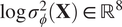 . The input multivariate time series are thus mapped to latent variables that are an eight-dimensional latent vector
$ \mathbf{z}\in {\mathrm{\mathbb{R}}}^8 $
 . The latent variables are subsequently sampled via the reparametrisation trick
$ \mathbf{z}={\mu}_{\phi}\left(\mathbf{X}\right)+{\sigma}_{\phi}\left(\mathbf{X}\right)\odot \boldsymbol{\varepsilon} $
 , where
$ \boldsymbol{\varepsilon} \sim \mathcal{N}\left(\mathbf{0},\mathbf{I}\right) $
 and
$ \odot $
 denote element-wise multiplication. The decoder,
$ {p}_{\theta}\left(\mathbf{X}|\mathbf{z}\right) $
 , performs the inverse reconstruction by employing a unidirectional LSTM for sequence generation. The latent vector
$ \mathbf{z} $
 is first expanded via a fully connected layer and repeated across the temporal dimension
$ p $
 to initialize the sequence. This sequence is processed by the unidirectional LSTM to reconstruct the temporal dynamics, followed by transposed convolutional layers to recover the original multivariate dimensions and local structure of the time series
$ \hat{\mathbf{X}} $
 . The architecture of the model is inspired by Mehmood et al. (Reference Mehmood, Yuan, Gong, Li, Hu, Li and Abbas2026).
The model parameters
$ \theta $
 and
$ \phi $
 are optimized by minimizing the
$ \beta $
 -VAE loss function (Higgins et al., Reference Higgins, Matthey, Pal, Burgess, Glorot, Botvinick, Mohamed and Lerchner2017) with mean squared error reconstruction loss and KL divergence regularization:

Training was run for up to 200 epochs using AdamW optimization (Loshchilov and Hutter, Reference Loshchilov and Hutter2019). To mitigate posterior collapse, we employ a monotonic annealing schedule for
$ \beta $
 , linearly increasing from
$ 0.01 $
 to
$ 1.0 $
 . For inference, each period was deterministically encoded as the variational posterior mean,
$ {\mathbf{z}}_i={\mu}_{\phi}\left({\mathbf{X}}_i\right) $
 providing a concise representation of the meteorological temporal dynamics. The latent vectors are L2-normalized to prioritize directional similarity over magnitude, then partitioned into
$ K $
 distinct weather clusters using Hierarchical Agglomerative clustering with Ward’s linkage (Ward, Reference Ward1963) and Euclidean distance.
2.4. Optimal configuration selection
The optimal configuration (
$ p $
 ,
$ K $
 ) is selected via grid search by maximizing a composite quality score
$ Q $
 . Drawing upon the multi-objective framework of Rana et al. (Reference Rana, Koprinska and Agelidis2016), the composite score aggregates six metrics, designed to balance statistical rigor in the latent space with physical interpretability and temporal coherence:

Structural quality is evaluated using the Silhouette score
$ S $
 (Rousseeuw, Reference Rousseeuw1987), which measures cluster cohesion and separation; the normalized Davies–Bouldin index
$ \tilde{D} $
 (Davies and Bouldin, Reference Davies and Bouldin1979), which evaluates intra-cluster similarity relative to inter-cluster separation; and the normalized Calinski–Harabasz index
$ \tilde{C} $
 (Caliński and Harabasz, Reference Caliński and Harabasz1974), which quantifies the ratio of between-cluster to within-cluster dispersion. Physical interpretability is validated using meteorological separability
$ \tilde{M} $
 , calculated as the log-normalized mean ANOVA F-statistic across wind speed, wind variability, and power output, while robustness is assessed through temporal coherence
$ T $
 , defined as the average within-cluster autocorrelation (Warren Liao, Reference Warren Liao2005), and distributional consistency (
$ H=1- JSD $
 ), which uses the Jennen–Shannon Divergence (Lin, Reference Lin1991) to penalize shifts in cluster proportions between training and testing sets. As detailed in Supplementary Table 4, a sensitivity analysis reveals a trade-off between these objectives: while structural metrics (
$ S $
 ,
$ \tilde{D} $
 ,
$ \tilde{C} $
 ) prefer compact representations with fewer clusters, physical and temporal metrics (
$ \tilde{M} $
 ,
$ T $
 ) improve with more clusters. To prioritize identifying distinct weather clusters, the composite weights were heuristically calibrated into two tiers. Primary structural and meteorological metrics (
$ S $
 ,
$ \tilde{D} $
 ,
$ \tilde{C} $
 ,
$ \tilde{M} $
 ) drive the core clustering behavior and were assigned dominant weights (0.2 each). Meanwhile, temporal coherence and distributional consistency (
$ T $
 ,
$ H $
 ) act as secondary regularization terms to prevent fragmented or unstable clusters, receiving lower weights (0.1 each). These generally pointed to similar results when clustering without a composite score, which is why they were combined to agree on final cluster parameters.
2.5. Gaussian process models
Following the assignment of meteorological periods to the
$ K $
 identified weather clusters, we model the relationship between atmospheric conditions and power generation using cluster-specific Gaussian Process regression (Williams and Rasmussen, Reference Williams and Rasmussen2005). GPs are particularly advantageous for tackling our “cold-start” problem because they operate nonparametrically and are highly data efficient, allowing them to adapt dynamically to limited target data. Crucially, unlike standard deterministic models, GPs inherently generate well-calibrated predictive distributions. For offshore WPF, this uncertainty quantification is an operational necessity, providing grid operators with the reliable risk margins required to securely manage reserve requirements and maintain system stability (Pinson, Reference Pinson2013). For each weather cluster
$ k $
 , a separate GP
$ {f}_k\left(\mathbf{x}\right)\sim \mathcal{GP}\left({m}_k\left(\mathbf{x}\right),{k}_k\left(\mathbf{x},{\mathbf{x}}^{\prime}\right)\right) $
 is trained to learn the cluster-dependent power curve, enabling each model to specialize in the distinct dynamics characterizing that specific weather type.
To capture both the overall period trajectory and immediate local conditions, we construct a 20-dimensional input vector
$ \mathbf{x}\in {\mathrm{\mathbb{R}}}^{20} $
 for each hourly forecast. This vector concatenates the 8-dimensional latent representation
$ \mathbf{z} $
 with 12 physical predictors: current wind speed and sea surface roughness, autoregressive lags
$ \left(t-1,t-2\right) $
 for both power and wind speed, and cyclical encodings (
$ \sin, \cos $
 ) of the hour, month, and wind direction.
To map this input to the target power output, the covariance function (kernel) must be tailored to the multi-scale physical reality of wind power generation. Standard applications of GPs in WPF frequently utilize the infinitely differentiable Squared Exponential (RBF) kernel, which effectively captures the smooth, theoretical aerodynamic relationship between wind speed and power (Rogers et al., Reference Rogers, Gardner, Dervilis, Worden, Maguire, Papatheou and Cross2020). However, real-world wind power curves contain high-frequency stochastic variations induced by local turbulence and wake effects, for which recent literature highlights the one-differentiable Matérn-
$ \nu =3/2 $
 is better suited (Prakash et al., Reference Prakash, Tuo and Ding2023). To explicitly capture both phenomena, we construct an additive composite kernel. The RBF component isolates the smooth, macroscopic baseline of the ideal power curve, while the Matérn-
$ \nu =3/2 $
 component captures the rougher, unpredictable atmospheric fluctuations:

where
$ {\sigma}_{f,k}^2 $
 controls the output variance. Both components utilize Automatic Relevance Determination (ARD), where
$ {\mathbf{\ell}}_k\in {\mathrm{\mathbb{R}}}^{20} $
 represents a vector of length scales. This allows the GP to automatically determine the relevance of each input feature for each specific cluster, for example, weighting lags more heavily in stable conditions versus turbulence features during storms.
Observation noise is modeled via a Gaussian likelihood with variance
$ {\sigma}_{n,k}^2 $
 , assuming
$ y={f}_k\left(\mathbf{x}\right)+\varepsilon $
 , where
$ \varepsilon \sim \mathcal{N}\left(0,{\sigma}_{n,k}^2\right) $
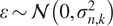 . Consequently, the covariance of the noisy observations is given by
$ {\mathbf{K}}_{y,k}={k}_k\left(\mathbf{x},{\mathbf{x}}^{\prime}\right)+{\sigma}_{n,k}^2I $
 . The complete hyperparameter set
$ {\theta}_k=\left\{{\sigma}_{f,k}^2,{\sigma}_{n,k}^2,{\mathbf{\ell}}_k^{\mathrm{RBF}},{\mathbf{\ell}}_k^{\mathrm{Mat}},{c}_k\right\} $
 is optimized by maximizing the exact marginal log-likelihood (MLL) of the observations. Using the noisy covariance
$ {\mathbf{K}}_{y,k} $
 , the MLL is defined as:

2.6. Transfer learning
To evaluate the cross-site generalization capability of the proposed framework, we apply a transfer learning strategy where the library of GP models is adapted to eight unseen target farms. This adaptation utilizes the fixed VAE encoder
$ {\phi}_S $
 and the set of cluster-specific GP priors, proceeding in three stages: latent projection, cluster alignment, and GP fine-tuning. First, the target meteorological time series
$ {\mathbf{X}}_t $
 are projected into the source latent space using the fixed source encoder
$ {\mathbf{z}}_T={\mu}_{\phi_S}\left({\mathbf{X}}_T\right) $
 . This enforces that target weather patterns are interpreted through the learned representation of the source domain. Each target period is then assigned to one of the
$ K $
 source weather clusters via a nearest-neighborhood classification in the latent space, utilizing the centroid from the source training set.
For each identified weather pattern
$ c\in \left\{1,\dots, k\right\} $
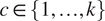 , we initialize a target GP
$ {f}_T^{(c)} $
 using the hyperparameters of the corresponding source GP,
$ {f}_S^{(c)} $
 . This initialization provides a strong prior on the temporal covariance structure of the power output. The kernel hyperparameters
$ {\theta}_k $
 are then optimized by maximizing the exact marginal log-likelihood on the available target training data
$ {\mathcal{D}}_{\mathrm{train}} $
 :

To assess data efficiency, we conducted experiments varying the data availability of the 2-year target datasets. Each target dataset is split into training fractions
$ \gamma \in \left\{\mathrm{0.1,0.2,0.3,0.4,0.5}\right\} $
 , simulating a “cold start” scenario where a newly commissioned wind farm has been operational for only a short period (ranging from ~2.4 to 12 months). The remaining
$ 1-\gamma $
 is reserved for testing.
3. Results
To evaluate the performance of our transfer learning framework under each data availability scenario, we benchmark our results against three no-transfer baselines. These are individual target farm-level GP and Neural Network (NN) models (experimental details are given in the Supplementary Appendix), which enable comparison with industry standards, and cluster-specific GPs trained from scratch, which helps to quantify the gain from fine-tuning the pre-trained models. We assess the predictive performance of these models using a combination of deterministic and probabilistic metrics (Xie et al., Reference Xie, Li, Li, Liu and Taukenova2023). Point predictions are evaluated using mean absolute error (MAE) and the coefficient of determination (
$ {R}^2 $
 ), uncertainty is quantified with the Continuous Ranked Probability Score (CRPS) and 95% Prediction-Interval Coverage Probability (PICP
$ {}_{95} $
 ). The formulas for the metrics are given in the Supplementary Appendix. To ensure comparability across wind farms, MAE and CRPS are expressed as a percentage of total capacity, while overall aggregated results are weighted by the number of time periods in each cluster to account for varying cluster sizes.
The time window with
$ p=6 $
 hours and
$ K=8 $
 clusters was identified as the best configuration, with a quality score of
$ Q=0.53 $
 . This provides the best trade-off, with cohesive clusters each with distinct meteorological patterns. Figure 3 shows the structural separation, where the eight-dimensional latent representation per training period is embedded into a two-dimensional plane using t-SNE (Maaten and Hinton, Reference Maaten and Hinton2008). Figure 4 illustrates the physical distinctiveness via mean wind speed distributions of each cluster: Clusters 1 and 5 capture calm periods, Cluster 2 isolates high-speed extremes, and Cluster 0 exhibits higher internal variance (likely characterizing transitional atmospheric states).
Latent space manifold visualized via t-SNE, showing the distribution of training periods across weather clusters.

Figure 3. Long description
The scatter plot visualizes high-dimensional data projected into two dimensions. The data points are organized into seven distinct but overlapping colored regions that form a circular distribution around a white central space.
* At the top center is a large light blue cluster extending vertically.
* Moving clockwise to the Northeast is a pink cluster.
* In the Southeast is a large red cluster.
* At the bottom center is a greyish-brown cluster with a horizontal orientation.
* In the Southwest is a large orange cluster.
* On the West side is a green cluster.
* In the Northwest is a purple cluster that overlaps with both the green and light blue regions.
Each region contains a high density of individual dots representing data points, with the boundaries of each cluster defined by a soft, translucent shaded outline of the same color. The title at the top reads Latent Space Manifold t - S N E.
Mean wind speed distribution of training periods by cluster (exemplified by seed 84).

Figure 4. Long description
The x-axis represents Mean Wind Speed in meters per second over Time Period, ranging from 0 to 25. The y-axis represents Density Probability, ranging from 0.000 to 0.200. Eight overlapping colored density curves represent Clusters 0 through 7.
* Cluster 1 (orange) has the highest peak at approximately 0.145 density around 6 meters per second.
* Cluster 2 (green) has a prominent peak at approximately 0.125 density around 12 meters per second.
* Cluster 6 (pink) peaks at approximately 0.120 density around 11 meters per second.
* Cluster 5 (brown) peaks at approximately 0.115 density around 8 meters per second.
* Cluster 4 (purple) and Cluster 0 (blue) show broader distributions peaking between 8 and 10 meters per second with densities around 0.100.
* Cluster 3 (red) peaks at approximately 0.100 density around 7.5 meters per second.
* Cluster 7 (grey) shows a lower, broader distribution peaking near 9 meters per second.
All curves originate near 0 on the x-axis and taper off toward 25 meters per second, with the majority of the data concentrated between 2 and 18 meters per second.
3.1. Quantitative results
The GP models achieved an MAE of
$ 3.68\%\pm 0.04\% $
 (24.4 MW;
$ {R}^2=0.981 $
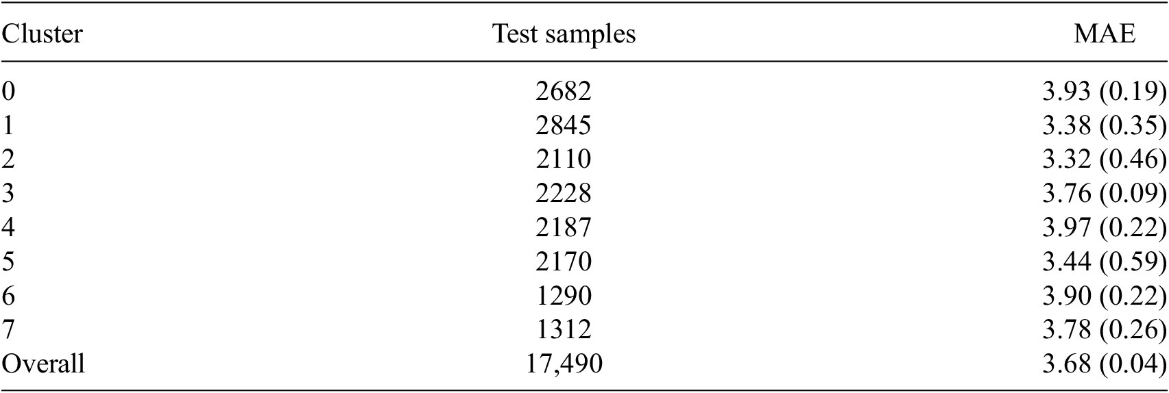
 ) when evaluated using 2 years of operational data across the six source farms (4:1 split). Table 1 shows the variability of performance for each cluster. Figure 5 shows that this is due to the specificity of each wind farm. Thus, the mixture of GPs captures a rich distribution of possible behaviors that can be flexible when adapted to new wind farms.
Cluster-level performance of source GP models, mean (std) across all target farms

Table 1. Long description
The table consists of three columns: Cluster, Test samples, and M A E (mean and standard deviation).
* Cluster 0: 2682 test samples, M A E 3.93 (0.19).
* Cluster 1: 2845 test samples, M A E 3.38 (0.35).
* Cluster 2: 2110 test samples, M A E 3.32 (0.46).
* Cluster 3: 2228 test samples, M A E 3.76 (0.09).
* Cluster 4: 2187 test samples, M A E 3.97 (0.22).
* Cluster 5: 2170 test samples, M A E 3.44 (0.59).
* Cluster 6: 1290 test samples, M A E 3.90 (0.22).
* Cluster 7: 1312 test samples, M A E 3.78 (0.26).
* Overall: 17,490 test samples, M A E 3.68 (0.04).
Performance of GP forecasts, disaggregated by wind farm and cluster.

Figure 5. Long description
A radar chart with eight axes labeled Cluster 0 through Cluster 7 arranged in a circle. The radial scale represents percentage values with concentric rings at 2.0 percent, 3.0 percent, 4.0 percent, and 5.0 percent.
Six wind farms are plotted as colored polygons:
* Baltic (teal): Shows a peak at Cluster 4, reaching approximately 4.5 percent, with lower values around 3.0 percent in other clusters.
* Beatrice (orange): Maintains a relatively tight, central profile, mostly staying between 2.5 percent and 3.5 percent.
* Gode (pink): Exhibits a prominent spike toward Cluster 4 and Cluster 7.
* Hornsea (light green): Shows its highest values at Cluster 7 and Cluster 4, extending beyond 4.0 percent.
* Ilnes (tan): Displays the most variance, with a sharp peak at Cluster 6 reaching near 5.0 percent and another high point at Cluster 2.
* Walney (grey): Follows a more uniform distribution, generally staying within the 3.0 percent to 3.5 percent range across most clusters.
The clusters are positioned as follows: Cluster 0 at 3 o’clock, Cluster 1 at 1:30, Cluster 2 at 12 o’clock, Cluster 3 at 10:30, Cluster 4 at 9 o’clock, Cluster 5 at 7:30, Cluster 6 at 6 o’clock, and Cluster 7 at 4:30.
A deterministic evaluation of the transfer learning approach for each cluster and proportion of available data is presented in Table 2, alongside baseline results. The metrics are averaged across the eight target farms. Fully disaggregated baseline results and probabilistic metrics are detailed in Supplementary Appendix D. As expected, when fine-tuning the pretrained GP models, we achieve superior generalization compared to training cluster-specific GP models from scratch. Notably, our framework requires under 5 months of local data (20% data capacity) to achieve an average MAE of 3.52%, outperforming the retrained models even when trained on a full year of data (MAE of 3.55%). Interestingly, Table 2 reveals that transferability strength varies significantly by meteorological cluster. For instance, Cluster 1 generalizes rapidly to new sites, achieving an MAE of 3.7% with only about 2.4 months of data. In contrast, Cluster 7 requires longer site-specific tuning, yielding an initial MAE of 5.8% at 2.4 months, which improves to 3.4% with 7.2 months. This suggests that while the source GPs successfully encode the broad dynamics of the respective weather patterns and take advantage of clusters that are easy to transfer, the meteorological phenomena associated with certain clusters are more location-dependent, necessitating a larger volume of local data for effective fine-tuning. Generally, adding data helps to reduce the variance in the fine-tuned location. Farm-level models allow a comparison with industrial baselines in Supplementary Tables 7 and 9. While single farm-level GPs outperform our framework with 10% of data, our approach achieves lower MAE across all subsequent data capacities. Interestingly, the farm-level GP baseline shows minimal improvement between 10% and 50% data capacity, improving only from an MAE of 3.84–3.56%. This early plateau highlights the inherent ability of GP models to generalize quickly with limited data and explains the plateau in our framework’s results between 40% and 50% capacity, when each cluster has more training samples.
Transfer learning performance by cluster and data capacity, mean (std) across all target farms

Table 2. Long description
The table evaluates performance using M A E and R-squared metrics.
Columns are organized by Data Capacity: 10 percent, 20 percent, 30 percent, 40 percent, and 50 percent. Each capacity contains two sub-columns: M A E and R-squared.
Rows include Clusters 0 through 7, followed by four summary rows: T L framework average, Farm-level G P average, Farm-level N N average, and Cluster-specific G Ps average.
Key data trends:
* For Cluster 0, M A E decreases from 4.4 at 10 percent capacity to 3.5 at 50 percent capacity, while R-squared remains stable at 0.96 to 0.97.
* Cluster 7 shows the highest initial M A E of 5.8 at 10 percent capacity, improving to 3.1 at 50 percent capacity.
* The T L framework average M A E improves from 4.34 to 3.22 as data capacity increases.
* Farm-level G P average maintains the highest R-squared values, ranging from 0.974 to 0.977 across all capacities.
* Cluster-specific G Ps average shows the most significant M A E improvement, dropping from 5.26 at 10 percent to 3.55 at 50 percent capacity.
Probabilistic metrics in Supplementary Tables 5 and 8 reveal our framework’s uncertainty quantification. The CRPS mirrors the performance improvements in deterministic results and remains lower than the MAE across all data capacities. This highlights a strength of our approach: even when the GPs’ predictive mean deviates from the actual observation, the probabilistic variance successfully expands to capture the true value. Furthermore, assessing the calibration of these bounds through the PICP
$ {}_{95} $
 shows our framework achieves a near-optimal PICP
$ {}_{95} $
 of 0.949 at 40% data capacity. In contrast, the baseline GP yields a PICP
$ {}_{95} $
 of 0.982 at 10% capacity (which increases with capacity), indicating less informative intervals. Finally, when benchmarked against an NN, our approach maintains superior performance across all data capacities, underscoring the data efficiency and robust generalisation of our GP-based transfer method over more complex deep learning architectures.
3.2. Farm-specific analysis
Breaking down performance by target farms shows how transferability varies according to the meteorological conditions unique to each farm. As shown in Table 3 for the Gemini wind farm, Clusters 0, 1, 2, 3, and 7 exhibit strong transferability. In these regimes, the pretrained GP models align well with local dynamics, all yielding MAEs equal or below 3.4% with ~5 months of fine-tuning data. Crucially, these clusters represent 66.7% of the evaluated time periods (at 20% data capacity), underscoring the operational benefit of the framework. Conversely, Clusters 4, 5, and 6 have lower transferability, suggesting that their associated weather patterns are specific to location, necessitating additional local data to refine the representations learned by the GPs.
Transfer learning performance by cluster and data capacity, mean(std), for the gemini wind farm

Table 3. Long description
The table is organized into seven columns. The first column lists Clusters 0 through 7, followed by T L framework average, Farm level G P average, Farm level N N average, and Cluster-specific G Ps average. The second column lists Test samples at 20 percent capacity. Columns three through seven represent Data capacity at 10 percent, 20 percent, 30 percent, 40 percent, and 50 percent, with each sub-headed by M A E.
Key data points include:
* Cluster 0: M A E decreases from 4.3 at 10 percent capacity to 3.0 at 50 percent capacity.
* Cluster 6: Shows the highest initial M A E of 6.7 at 10 percent capacity, dropping to 3.5 at 50 percent capacity.
* Cluster 2: Consistently shows the lowest M A E, starting at 2.4 and ending at 1.9.
* T L framework average: Shows a steady improvement from 4.29 (0.14) to 2.98 (0.03).
* Farm level G P average: Ranges from 3.5 (0.06) to 3.27 (0.07).
* Farm level N N average: Ranges from 4.29 (0.10) to 3.30 (0.11).
* Cluster-specific G Ps average: Improves from 5.06 (0.11) to 3.31 (0.03).
Values are presented as mean with standard deviation in parentheses.
4. Discussion
The proposed framework demonstrates that weather-specific transfer learning reduces data requirements for accurate forecasting in European offshore wind farms. To scale this approach, future work will pursue two main avenues. First, scaling for longer lead times, which will require factorizing the time-series data, allowing for longer contexts that select key information for precise forecasting. This should pave the way for geographic transfer of clusters into more diverse climate zones by identifying the parts of the time series that will be crucial in forecasting future patterns, and thus overcoming the shortcoming of our approach for clusters that need longer fine-tuning. In a second avenue, using real-world data will bring multiple challenges. These include incorporating turbine specifications and wake effect modeling to account for intra-farm heterogeneity, as well as handling less granular data, since early-stage collection often contains missing data points and irregular observations. This research direction will counter the biased outcome of using synthetic data that does not necessarily correspond to operational environments. Additionally, implementing this methodology at production would require cross-validation of the weights given to each metric used to create the composite score to avoid clustering errors. Collectively, these advancements pave the way toward a dynamic WRA tool capable of generating rapid, location- and configuration-specific forecasts without the need for lengthy initial data investment, thus accelerating future investments into offshore wind farms, and allowing the growth of cheaper, greener energy.
Supplementary material
The supplementary material for this article can be found at http://doi.org/10.1017/eds.2026.10055.
Acknowledgments
The authors would like to thank the anonymous reviewers and meta-reviewers for providing constructive and helpful remarks. Chloé Hashimoto-Cullen would like to thank Sylvain Le Corff for proofreading the manuscript. Chloé Hashimoto-Cullen is co-funded by the European Union’s Horizon Europe research and innovation program Cofund SOUND.AI under the Marie Sklodowska-Curie Grant Agreement No. 101081674. Views and opinions expressed are, however, those of the author(s) only and do not necessarily reflect those of the European Union or the granting authority. Neither the European Union nor the granting authority can be held responsible for them.
Author contribution
Conceptualization: D.W., C.C., B.G.; Data curation: D.W.; Formal analysis: D.W., C.C.; Methodology: D.W., C.C., B.G.; Supervision: C.C., B.G.; Validation: D.W., C.C., B.G.; Visualization: D.W.; Writing—original draft: D.W., C.C.; Writing—review and editing: D.W., C.C., B.G.
Competing interests
The authors declare none.
Data availability statement
The code and data used in this study are archived on Zenodo at https://doi.org/10.5281/zenodo.20665331.
Funding statement
This research received no specific grant from any funding agency in the public, commercial, or not-for-profit sectors. This research was undertaken as part of the lead authors MSc AI for Sustainable Development at UCL.
Provenance statement
This article is part of the Climate Informatics 2026 proceedings and was accepted in Environmental Data Science on the basis of the Climate Informatics peer review process.




 Open access

