2.1. Experimental set-up

The experimental set-up included air and water delivery systems as well as a flow apparatus. The air delivery system included an Atlas Copco compressor (model GA37FF) and the air flow rate was measured using an MCRH 5000 ALICAT mass flow controller. The water delivery system included a nitrogen bottle to purge water from a pressurized tank as well as a PCD-100-PSIG dual valve pressure controller from ALICAT. For all test conditions, the reservoir pressure was fixed at 62.1 kPa gauge. The liquid flow rate was calibrated following the procedure detailed in Rostami et al. (Reference Rostami, Li and Kheirkhah2023). It was measured that the above reservoir pressure corresponded to an injection of 13.8 grams of water per minute (cf. 21.9 grams per minute in Rostami et al. Reference Rostami, Li and Kheirkhah2023). The reduced flow rate of water in the present study was necessary to produce a dilute spray, which was required for 3-D measurements. Both the air and water delivery systems were identical to those used in our earlier study (Rostami et al. Reference Rostami, Li and Kheirkhah2023).

The flow apparatus included a diffuser section, a settling chamber and a nozzle, which are shown in figure 1. The area ratio of the diffuser was about four, and the settling chamber was equipped with five equally spaced mesh screens, identical to Kheirkhah & Gülder (Reference Kheirkhah and Gülder2013), Kheirkhah (Reference Kheirkhah2016), Mohammadnejad, Saca & Kheirkhah (Reference Mohammadnejad, Saca and Kheirkhah2022) and Rostami et al. (Reference Rostami, Li and Kheirkhah2023). Compared with these studies, the nozzle section was different and was similar to Krebbers et al. (Reference Krebbers, Mohammadnejad, Rostami and Kheirkhah2023). Specifically, the nozzle section included a Delavan pressure swirl atomizer (model S0075-60S1) and a swirler, with details shown in the inset of figure 1. The utilized pressure swirl atomizer is similar to that used in Rostami et al. (Reference Rostami, Li and Kheirkhah2023). It should be highlighted that in our previous study, the background turbulent flow characteristics were adjusted using perforated plates. However, in the present study, a radial swirler generated the background turbulent flow. In past studies, e.g. Wang, Bauer & Gülder (Reference Wang, Bauer and Gülder2019), the combination of the nozzle and a combustion chamber was referred to as the gas turbine model combustor. Compared with Krebbers et al. (Reference Krebbers, Mohammadnejad, Rostami and Kheirkhah2023) and Wang et al. (Reference Wang, Bauer and Gülder2019), improving the quality of our measurements and accommodating a relatively large field of view (FOV), the combustion chamber was removed. Also compared with these past studies, water (instead of Jet A-1) was the working fluid and the flow was non-reacting in the present study.

Figure 1.

The flow apparatus, which is composed of a diffuser section, a settling chamber and a nozzle. The inset on the right-hand side is the technical drawing of the nozzle cross-section as well as a picture of the atomizer tip.

2.2. Diagnostics

Three diagnostics, namely, AIPI, stereoscopic particle image velocimetry (SPIV) and shadowgraphy were separately used in the present study. The schematic arrangement of these diagnostics are presented in figure 2(a–c), respectively. The dimensions in the figure are not to scale. The details of the utilized diagnostics are discussed in the following.

Figure 2.

The utilized diagnostics. Panels (a–c) are the schematic arrangement of AIPI, SPIV and shadowgraphy technique, respectively. The dimensions are not to scale.

2.2.1. Astigmatic interferometric particle imaging

The AIPI technique was used for the simultaneous measurement of the 3-D location of the spray droplets and their corresponding diameter. The hardware of the AIPI technique consisted of an Nd:YAG dual cavity pulsed laser (model: Evergreen PIV 200), volume illumination optics, an Andor's Zyla 5.5 sCMOS camera (C1) and collection optics for C1. The laser produced a 532 nm laser beam, with a beam diameter of about 5 mm. The energy of the laser was measured using a pyroelectric energy detector from Gentec Electro-Optics Inc. (model: QE25LP-S-MB-QED-INT-D0), with the maximum energy of the laser being about 200 mJ per pulse. For all experiments, the laser was operated at 45 % of its maximum energy to avoid saturation of the AIPI images. The laser beam was converted into a laser slab using the volume illumination optics (see the blue dashed box in figure 2a). The volume illumination optics included the LaVision divergent sheet optics, which were two spherical lenses (SL1 and SL2), a cylindrical lens (CL1) with a focal length ($\,f$) of $-20$ mm, and a spherical lens (SL3 from Thorlabs, model LA1145-AB-ML) with $f = 75$ mm. It is important to note that the combination of SL1, SL2 and CL1 allowed for generating a rectangular laser slab, with a maximum thickness of about 10 mm. However, such thickness was not sufficient for the purposes of the volumetric illumination of the spray in the present study, and as such, SL3 was additionally installed. This last spherical lens allowed for increasing the thickness of the illuminated volume from about 10 to 60 mm near the nozzle centreline, which was 1060 mm distant from the centreline of SL3. For presentation purposes, this distance is shortened in figure 2(a). The collection optics included a $532\pm 10\,{\rm nm}$ bandpass filter (BF1), a Macro Sigma objective lens (OL1, with $f = 105$ mm) and a cylindrical lens (CL2, with $f = 250$ mm). The integration of CL2 with OL1 results in the formation of two focal planes P1 and P2 (see figure 2), with P1 being outside of the illumination volume. These two focal planes are formed since the angles of the light refraction along the power and axis meridians of the cylindrical lens are different. The focal length of CL2 is identical to that used in past studies; see, for example, Shen et al. (Reference Shen, Coetmellec and Brunel2012), Wen et al. (Reference Wen, Wu, Zhuo and Wu2021) and Wu et al. (Reference Wu, Wen, Zhuo, Wang and Wu2022). Using the ray transfer matrix method presented in Zhuo et al. (Reference Zhuo, Wu, Wen, Lin and Wu2022), it was confirmed that the selected focal length of CL2 allows for resolving droplets in the entire measurement volume with sufficient sensitivity. The CL2 lens was installed on a rotary mount (model CLR1 from Thorlabs) that allowed us to rotate CL2 with respect to the axis of the collection optics; see figure 2(a). The CL2 lens was positioned between the camera sensor and OL1 to create an astigmatic effect, similar to the studies of Wen et al. (Reference Wen, Wu, Zhuo and Wu2021). The axis of the collection optics was positioned such that it made an angle of $\theta = 70^{\circ }$ with the laser beam axis; see the angle between the dotted-dashed lines in figure 2(a). This angle was selected as it yielded the best clarity of interferometric images, following Sahu (Reference Sahu2011). For each test condition (discussed later), 2000 AIPI images were acquired with the acquisition frequency of 10 Hz.

A Cartesian coordinate system was used to locate the AIPI region of interest. This coordinate system is shown by $x$, $y$ and $z$ axes in figure 3. The origin of this coordinate system coincides with the intersection of the spray injector centreline ($\kern0.7pt y$-axis) and the exit plane of the nozzle. The $z$-axis coincides with the axis of the collection optics and points towards the camera sensor. The $x$-axis is perpendicular to both $y$ and $z$ axes. The AIPI region of interest is shown by the transparent green box in figure 3. This region extends from $-$42.5 to $-$7.5, 43.2 to 71.2 and $-$30.0 to 30.0 mm, along the $x$, $y$ and $z$ axes, respectively. Thus, the AIPI volume of interest ($V_{AIPI}$) is $35\times 28\times 60=58\,800\,\mathrm {mm}^3$. It should be noted that the AIPI region of interest is intentionally selected to be near a sufficiently dilute region of the spray. This was necessary to ensure the accuracy of the 3-D spray measurements by AIPI, with details discussed in § 3.1.

Figure 3.

The green box, blue slab and red slab present the AIPI, SPIV and shadowgraphy regions of interest, respectively. $(x,y,z)$ is the coordinate system used for the AIPI and $(x',y,z')$ is that used for the SPIV and the shadowgraphy techniques. The axes in the figure match those in figure 2.

2.2.3. Shadowgraphy

The shadowgraphy technique was used to understand the effects of the swirling flow on the spray formation and large droplets breakup. The shadowgraphy hardware included a backlight LED lamp (model NL-360ARC from Neewer) and a Photron Fastcam Nova S12 high-speed camera (C4 in figure 2c) equipped with a Macro Sigma lens, with $f = 105$ mm and its aperture size was set to $f/2.8$. The shadowgraphy images were captured for a duration of 1 s with the acquisition frequency of 10 kHz. The camera exposure time was set to $20\,\mathrm {\mu }$s. The FOV of the shadowgraphy imaging was 64 mm along the $x'$-axis and 64 mm along the $y$-axis. The depth of field (DOF) for the shadowgraphy camera was calculated using the formulation from Gross, Blechinger & Achtner (Reference Gross, Blechinger and Achtner2008), which is given by

(2.1)\begin{equation} {DOF} = \frac{2of^2N\tilde{c}(o-f)}{f^4 - \tilde{c}^2N^2(o-f)^2}, \end{equation}

where $\tilde {c}$ is the camera sensor size, $N$ is the aperture number and $o$ is the distance between the camera sensor and the plane of focus. In the present study, $\tilde {c}$ and $o$ were $20\,\mathrm {\mu }{\rm m}$ and 500 mm, respectively. Substituting the above values in (2.1), the DOF was calculated and was about 2 mm. The shadowgraphy FOV is shown by the red slab in figure 3.

2.3. Test conditions

In total, eight test conditions were examined with details presented in table 1. For all test conditions, the liquid flow rate was kept constant. The mean bulk flow velocity of the air flow ($U_{b}$) was estimated by dividing the set air flow rate to the exit area of the nozzle section, which is the area of a circle with diameter $D=28.0\,\mathrm {mm}$, subtracted by the surface area of the Delavan injector at its exit; see the inset of figure 1. In the present study, $U_{b}$ was varied from 6.1 to $27.4\,\mathrm {m}\,\mathrm {s}^{-1}$, with the corresponding values tabulated in the first column of table 1. It is important to note that, for $U_{b} < 6.1\,\mathrm {m}\,\mathrm {s}^{-1}$, the spray was too dense and the AIPI was not performed for these velocities. However, qualitative analysis of the spray was possible using the shadowgraphy technique, and as a result, in addition to the mean bulk flow velocities presented in table 1, shadowgraphy experiments were performed for $U_{b}= 0\,\mathrm {m}\,\mathrm {s}^{-1}$ (which corresponds to no background air flow). The Reynolds number estimated based on the mean bulk flow velocity was calculated using $Re_D=U_{b}D/\nu$, with $\nu$ being the kinematic viscosity of the air at the laboratory temperature. The values of $Re_D$ are tabulated in the second column of table 1.

Table 1.

Test conditions.

The background turbulent flow characteristics were estimated at the intersection of the SPIV FOV and the AIPI region of interest. This intersection region extends from $-$39.9 to $-$7.0 and 43.2 to 71.2 mm, along the $x'$ and $y$ axes, respectively. The r.m.s. of the streamwise (along the $y$-axis) velocity fluctuations was averaged inside the above region, referred to as $\tilde {u}_{rms}$, and listed in the third column of table 1. The integral length scale was calculated using the autocorrelation of the streamwise velocity fluctuations, following the formulations presented in Kheirkhah & Gülder (Reference Kheirkhah and Gülder2015) and Kheirkhah (Reference Kheirkhah2016). Similar to these studies, the calculation of the integral length scale at spatial locations corresponding to $y \gtrsim 60.0$ mm was not possible since the autocorrelation of the velocity data did not attain a zero value. As such, the integral length scale was calculated in the intersection region of SPIV and AIPI and for $43.2\,\mathrm {mm} \lesssim y \lesssim 60.0\,\mathrm {mm}$. The values of $\varLambda$ are listed in the fourth column of table 1. The Taylor ($\lambda$) and Kolmogorov ($\eta$) length scales were calculated using $\lambda = \varLambda (\tilde {u}_{rms} \varLambda /\nu )^{-0.5}$ and $\eta = \varLambda (\tilde {u}_{rms} \varLambda /\nu )^{-0.75}$. It should be noted that, in the formulations used for the estimation of $\lambda$ and $\eta$, it is inherently assumed that the normalized dissipation rate of the turbulent kinetic energy is unity. It is acknowledged this is not necessarily a fixed parameter (see, for example, Vassilicos Reference Vassilicos2015) and can feature dependence on the type of turbulence generator, where it is measured, and $Re_\lambda$; see Burattini, Lavoie & Antonia (Reference Burattini, Lavoie and Antonia2005). In the present study, similar to past investigations that studied the droplet-laden flows (see, for example, Sumbekova et al. Reference Sumbekova, Cartellier, Aliseda and Bourgoin2017), the normalized dissipation rate of the turbulent kinetic energy was taken as unity. The values of $\lambda$ and $\eta$ are presented in the fifth and sixth columns of table 1, respectively. For all test conditions, $\tilde {u}_{rms}$ varied from about 1.0 to $4.4\,\mathrm {m}\,\mathrm {s}^{-1}$, while the integral length scale was nearly constant ($\varLambda = 7.6-7.8\,\mathrm {mm}$). The Taylor and Kolmogorov length scales varied from about 160 to $347\,\mathrm {\mu }{\rm m}$ and from 23 to $73\,\mathrm {\mu }{\rm m}$, respectively.

The formulation provided in Lefebvre & McDonell (Reference Lefebvre and McDonell2017) and the AIPI data were used to estimate the Sauter mean diameter (SMD) of the spray droplets. The values of the SMD are listed in the seventh column of the table. The AIPI data was also used to estimate the mean droplet diameter ($\bar {d}$), which is listed in the eighth column of the table. For the conditions tested in the present study, SMD and $\bar {d}$ varied from 67 to $95\,\mathrm {\mu }{\rm m}$ and 37 to $57\,\mathrm {\mu }{\rm m}$, respectively. It should be noted that, since the calculation of the SMD involves the volume-to-surface area ratio of the droplets, it is anticipated that the SMD be skewed toward the diameter of large droplets, resulting in the larger values of the SMD compared with $\bar {d}$. In summary, comparison of the results presented in the sixth to eighth columns of table 1 shows that the size of the spray droplets are of the order of the Kolmogorov length scale tested in the present investigation. It is noted that given the differences in the water flow rate and the background turbulence between the present study and those of our previous investigation (see Rostami et al. Reference Rostami, Li and Kheirkhah2023), the mean diameter of the droplets in this study are larger than those in Rostami et al. (Reference Rostami, Li and Kheirkhah2023), which varied from 30 to $38\,\mathrm {\mu }{\rm m}$.

Of prime importance in studying the particle-laden flows are the Taylor-length-scale-based Reynolds number, Stokes number and the spray volume fraction ($\phi _{v}$). The Taylor-length-scale-based Reynolds number was estimated using $Re_\lambda = \tilde {u}_{rms} \lambda /\nu$, with the corresponding values listed in the ninth column of table 1. In the present study, $Re_\lambda$ varies from about 22 to 47, which are relatively moderate values compared with past particle-laden flow studies; see, for example, Sumbekova et al. (Reference Sumbekova, Cartellier, Aliseda and Bourgoin2017). Following Reade & Collins (Reference Reade and Collins2000), the Stokes number was calculated using

(2.2)\begin{equation} St=\frac{1}{18}\frac{\rho_{W}}{\rho_{A}}\left(\frac{d}{\eta}\right)^{2}, \end{equation}

where $\rho _{W}$ and $\rho _{A}$ are the water and air densities both estimated at the laboratory temperature ($21\,^{\circ }{\rm C}$) and pressure (1 atm). In (2.2), $d$ is a characteristic size for the droplet diameter. In the present study, the mean droplet diameter was used for the estimation of the Stokes number. The values of the Stokes number are tabulated in the tenth column of table 1 and vary from about 34 to 142, which are relatively large compared with those tested in the literature. It is important to note that in the present study, the mean droplet diameter is larger than the Kolmogorov length scale, and following the studies of Xu & Bodenschatz (Reference Xu and Bodenschatz2008) and Monchaux, Bourgoin & Cartellier (Reference Monchaux, Bourgoin and Cartellier2012), the Kolmogorov time scale may not be appropriate for calculating the Stokes number. Specifically, the above studies suggested using the droplet diameter instead of the Kolmogorov length scale for calculating the Stokes number. Using the formulation proposed in Xu & Bodenschatz (Reference Xu and Bodenschatz2008) and Monchaux et al. (Reference Monchaux, Bourgoin and Cartellier2012) led to the Stokes number varying from about 40 to 104. Either of the calculations discussed above leads to values of the Stokes number that are substantially larger than those examined in previous studies. Nonetheless, using either of the definitions of the Stokes number yields similar conclusions. In the present study, (2.2) was used for estimation of the Stokes number, facilitating comparisons with the results of Rostami et al. (Reference Rostami, Li and Kheirkhah2023).

The spray volume fraction was estimated using the formulation in Elghobashi (Reference Elghobashi1994), which is given by

(2.3)\begin{equation} \phi_{v} = \bar{n}\frac{V_{d}}{V_{AIPI}}, \end{equation}

where $\bar {n}$ is the mean number of droplets within the volume of the AIPI region of interest (see the green box in figure 3) and $V_{d}$ is the volume occupied by an individual droplet. For each test condition, the number of droplets, $n$, was calculated using the AIPI technique and was averaged over all collected images. The volume occupied by a droplet was approximated by $V_{d} = ({\rm \pi} /6) \bar {d}^{3}$. The values of $\phi _{v}$ are listed in the eleventh column of table 1. In the present study, the spray volume fraction varied from $0.35\times 10^{-6}$ to $0.74\times 10^{-6}$, rendering the tested sprays dilute, as suggested in Elghobashi (Reference Elghobashi1994).

3.1. Three-dimensional positioning and sizing of droplets

A cropped view of a representative image from AIPI is shown in figure 4(a) that corresponds to the test condition with $U_{b}=15.2\,\mathrm {m}\,\mathrm {s}^{-1}$. As can bee seen, the interferometric images of the droplets are oriented elliptical regions that feature slanted fringes. Similar to the present study, such elliptical interferometric images of droplets are reported in previous investigations; see, for example, Shen, Coetmellec & Brunel (Reference Shen, Coetmellec and Brunel2013) and Wen et al. (Reference Wen, Wu, Zhuo and Wu2021). A sample region is highlighted by the box in figure 4(a) and is enlarged and shown in figure 4(b). The Canny edge detection algorithm in MATLAB was used to obtain the boundary of the elliptical regions, with a sample ellipse shown in figure 4(b). The centres of the elliptical regions were obtained fitting an ellipse to the detected elliptical regions using the least square method, and then finding the centres of the fitted ellipses. It is important to note that a discrepancy exists between the true $x$ and $y$ coordinates of the droplets and the centre of the ellipses. This discrepancy was obtained and corrected, with the correction procedure presented in Appendix A.

Figure 4.

Panel (a) is a cropped AIPI raw image. Panel (b) is a sample interference pattern from (a). Panel (c) is the inset of (b) corresponding to the red rectangle in (b). Panel (d) is the 2-D fast Fourier transform magnitude for the interference pattern shown in (c). Overlaid on (d) are the $x''$ and $y''$ axes that are the axes corresponding to the power and axis meridians of the cylindrical lens CL2. In panel (d) the angle between the line that connects the two peaks and the $y''$-axis is $\alpha$. (e) The red solid curve presents the relation between $\alpha$ and the depth of the spray droplets obtained from (3.1). In (e), the blue circular data points are obtained from the calibration experiments.

The depth of the droplets (i.e. the droplets $z$ coordinate) was obtained using the ray transfer matrix method, which is elaborated in Wen et al. (Reference Wen, Wu, Zhuo and Wu2021). To this end, the elements of the ray transfer matrix for the rays propagating along the power meridian and axis meridian of CL2 were obtained. Then, these elements along with (13) in Wen et al. (Reference Wen, Wu, Zhuo and Wu2021) were used to obtain the depth of the droplets given by

(3.1)\begin{equation} \frac{c-b-z}{c-a-z} ={-}\frac{M_1}{M_2}\frac{\tan(\alpha)}{\tan(\alpha_0)}, \end{equation}

where $a$ and $b$ are the distances between the surface of the bandpass filter shown in figure 2(a) and the focal planes 1 and 2, respectively; $c=210\,\mathrm {mm}$ is the distance between the origin of the coordinate system and the surface of the bandpass filter; $c-a-z$ and $c-b-z$ are the distances along the $z$-axis between a droplet with the depth of $z$ and focal planes 1 and 2, respectively. Please note that the choice of bandpass filter surface for the calculations is arbitrary and choosing other reference planes does not influence the values of $z$. This is because $c-a$ and $c-b$ that appear in (3.1) are the distances between the focal planes and the origin of the coordinate system that are fixed in the experiments. In (3.1), $M_1$ and $M_2$ are the magnification ratios for imaging at planes 1 and 2, respectively. Separate experiments (with laser turned off and in the absence of spray and air flow) were performed to obtain the above parameters, with details of these experiments discussed in Appendix B. In the present study, the values of $a$, $b$, $M_1$ and $M_2$ were 160 mm, 200 mm, 0.53 and 0.54, respectively. Here $\alpha _0$ is the angle that the power meridian of the cylindrical lens (CL2) makes with the $x$–$z$ plane. This angle was set to ${\rm \pi} /4$ using the CL2 mount. In (3.1), $\alpha$ depends on the orientation of the fringe patterns, with details of the calculation discussed below.

To calculate $\alpha$, first the angle between the slanted fringes (see, for example, those in figure 4(b)) and the $x$-axis was obtained. This angle is referred to as $\gamma$. To calculate $\gamma$, first, a rectangular region highlighted with the red square in figure 4(b) was selected. This region is enlarged and shown in figure 4(c). Then, a 2-D fast Fourier transform (FFT) was applied to the data in this region, with the results presented in figure 4(d). To help elaborate the calculation of $\alpha$, the power meridian ($x''$) and axis meridian ($\kern0.7pt y''$) of CL2 were overlaid on figure 4(d). As can be seen in figure 4(d), two peaks (see the blue dots) are identified. The angle between the line that connects these two peaks (the brown dashed line) and the $f_y$ axis is referred to as $\gamma$ (see Gonzalez & Woods Reference Gonzalez and Woods2018). The angle between this line and the $y''$-axis is referred to as $\alpha$. The variation of $\alpha$ vs $z$ was obtained using (3.1) and is presented by the solid red curve in figure 4(e). As can be seen, the variation of $\alpha$ features an abrupt change at $z=10$ mm. The location of this abrupt change corresponds to focal plane 2 and is due to the change in the sign of $\tan (\alpha )$ in (3.1). That is, at $z = c-b=10\,\mathrm {mm}$, $\tan (\alpha )$ becomes zero. In addition to the predictions from (3.1), separate calibration experiments (detailed in Appendix B) were performed to experimentally obtain the relation between the depth of the droplets and $\alpha$. The results of these calibration experiments are overlaid on figure 4(e) using the blue solid circular data points. As can be seen, the results obtained from (3.1) and those from the calibration experiments match, suggesting that the formulation in (3.1) can allow for predicting the droplets depth using $\alpha$.

Once the $z$ location of a droplet was calculated using the above procedure, its diameter was obtained from the formulation proposed in Wen et al. (Reference Wen, Wu, Zhuo and Wu2021), which is given by

(3.2)\begin{equation} d=F(z)\dfrac{2\lambda_{{L}}}{s} \left[\cos\left(\dfrac{\theta}{2}\right)+\dfrac{m\sin\left(\dfrac{\theta}{2} \right)}{\sqrt{m^{2}-2m\cos\left(\dfrac{\theta}{2}\right)+1}}\right]^{{-}1}, \end{equation}

where $F(z)$ represents the dependence of the droplet diameter on its position along the $z$-axis. Here $F(z)$ is given by

(3.3)\begin{equation} F(z)=\dfrac{1}{\sqrt{\left[\dfrac{\cos(\alpha_0)}{M_1(c-a-z)}\right]^2+ \left[\dfrac{\sin(\alpha_0)}{M_2(c-b-z)}\right]^2}}. \end{equation}

In (3.2), $\lambda _{{L}}$ is the wavelength of the AIPI laser, $s$ is the fringe spatial spacing, with a sample shown in figure 4(c), and $m$ is the index of refraction for distilled water, which is 1.33 as provided in Hardalupas et al. (Reference Hardalupas, Sahu, Taylor and Zarogoulidis2010). The uncertainties associated with measuring the droplet depth and diameter were estimated and the details are presented in Appendix C. These uncertainties depend on the imaging resolution, characteristics of the optics (such as focal length, magnification ratios and the distance between the focal planes), as well as the characteristics of the fringe patterns (such as their orientation and spacing). It was obtained that the maximum relative uncertainties in estimating the droplet depth and most probable diameter are about 13 % and 27 %, respectively.

Though the above procedure allows for estimating the droplets location and size, care must be taken in using the AIPI technique and also reducing the acquired images. Three limitations are of importance and are discussed here. First, it should be noted that this 3-D measurement technique, with details discussed above, can be applicable to dilute sprays but may not be applied to dense sprays such as those used in our previous investigation (Rostami et al. Reference Rostami, Li and Kheirkhah2023). Generally, sprays with significant overlap between the interferometric patterns of droplets (see an example in figure 5a) reduce the ability of the AIPI in resolving the location and size of the droplets. However, reliable 3-D measurements can yield an improved understanding of the sprays compared with the 2-D counterparts, provided the measurements are performed in a dilute spray environment, which is relevant to the present investigation. Second, too large droplets (larger than $200\,\mathrm {\mu }{\rm m}$, see an example of a large droplet interferometric pattern in figure 5b) cannot be resolved. The procedure for removing too large droplets and those with significant overlap of the interferometric patterns from the analysis of the AIPI data is discussed in Appendix D. Third, the fringe patterns may not be fully developed inside focusing volume(s), and the measurement of the diameter for these droplets is not possible. In the present study, only the focusing plane P2 is located inside the illumination region. The focusing depth around P2 is about 1 mm that is significantly smaller than the total depth of the measurements (60 mm). It is important to note that the AIPI is capable of measuring the location of droplets positioned at P2 (see an example in figure 5c), but the diameter of those droplets cannot be measured. The $z$ location of the droplets in P2 equals $c-b$. Specifically, at $z = c-b$, (3.1) yields $\alpha = 0$. Thus, the 3-D position of the droplets located in plane P2 can be obtained but their diameter cannot be calculated.

Figure 5.

Panel (a) presents significantly overlapping astigmatic interferometric images of droplets. Panel (b) presents astigmatic interferometric images of too large droplets, which cannot be resolved using the AIPI technique. Panel (c) presents an astigmatic interferometric image of a droplet located at the focal plane P2.

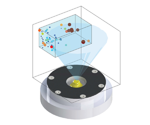
Acknowledging the above limitations, the 3-D position and the diameter of the droplets were obtained for all test conditions. Figure 6(a) shows a representative 3-D distribution of the droplets as well as their diameter. The results presented in the figure are for the test condition with $U_{b}=6.1\,\mathrm {m}\,\mathrm {s}^{-1}$. To facilitate understanding the location of the droplets with respect to the spray, the spray cone of the utilized atomizer was overlaid on figure 6(a). The cone angle of the spray is $60^{\circ }$ in the absence of swirling co-flow and is provided by the manufacturer. The top and side views of the results in figure 6(a) are shown in figures 6(b) and 6(c), respectively. As can be seen, the large droplets are located at the periphery of the spray. It is speculated that the reason that a few of the identified droplets are positioned outside of this cone is the presence of the turbulent swirling co-flow, which is expected to increase the spray cone angle, as also reported in past investigations; see, for example, Rajamanickam & Basu (Reference Rajamanickam and Basu2017). The location of the droplets in three dimensions was used for identifying the clusters and voids, with relevant details discussed in the following subsection.

Figure 6.

Panel (a) is the 3-D distribution of the droplets and the droplets diameter. Panels (b,c) are the top and side views of the 3-D distribution shown in (a). The transparent blue box presents the AIPI volume of interest. The results correspond to the test condition with $U_{b}=6.1\,\mathrm {m}\,\mathrm {s}^{-1}$.

3.2. Clusters and voids identification in the 3-D space

The spatial distribution of the droplets in 3-D space was used to identify the clusters and voids. Using the 3-D position of the droplets centre along with the ‘Voronoin’ function in MATLAB, the 3-D Voronoï cells were obtained first. This was followed by removing the cells intersecting with the boundaries of the AIPI volume of interest. As a representative example, for the droplets identified and presented in figure 6, the Voronoï cells were obtained, those intersecting with the AIPI region-of-interest boundaries were removed, and the remaining cells are shown in figure 7(a). The 3-D position of all detected droplets were used to identify clusters and voids. For joint analysis of the droplet diameter and cluster volume, the droplets with detectable diameter that reside within the clusters/voids were used for the analysis.

Figure 7.

Panel (a) is the Voronoï cells generated using the 3-D spatial distribution of droplets in figure 6. Panel (b) presents the p.d.f. of the local Voronoï cells' volumes normalized by their local mean value for the test condition with $U_{b} =6.1\,\mathrm {m}\,\mathrm {s}^{-1}$. Overlaid on (b) is the p.d.f. of a random distribution of the droplets (see the black solid curve). Panel (c) presents the identified clusters (blue) and voids (green).

Once the Voronoï cells were obtained, the volumes of the cells were calculated using the ‘convhulln’ function in MATLAB. Compared with the particle-laden flow studies in which the particles are initially and relatively uniformly distributed in wind tunnels, in many engineering applications, the particles/droplets feature a biased distribution in space and, as a result, several regions in the 3-D space feature a relatively large concentration of the droplets. In the present study, the pressure swirl atomizer creates an inverted cone of droplets. Such a distribution of droplets leads to biased Voronoï cell volumes, and this bias was removed following the procedure described below, which is similar to that used in Sumbekova et al. (Reference Sumbekova, Cartellier, Aliseda and Bourgoin2017) and Rostami et al. (Reference Rostami, Li and Kheirkhah2023) for 2-D Voronoï cells. To this end, the mean of the local Voronoï cell's volume ($\bar {V}(x,y,z)$) was obtained first. To estimate $\bar {V}(x,y,z)$, the AIPI volume of interest was divided into several voxels with a length, width and height of $\Delta x = 4\,\mathrm {mm}$, $\Delta y=4\,\mathrm {mm}$ and $\Delta z=6\,\mathrm {mm}$, respectively. Then, the volume of the Voronoï cells corresponding to the droplets located within each of these voxels was obtained for all frames and then averaged for each test condition. To identify the clusters, first, the $\mathrm {p.d.f.}(V/\bar {V})$ was obtained, with that for the mean bulk flow velocity of $6.1\,\mathrm {m}\,\mathrm {s}^{-1}$ shown in figure 7(b) using the circular date symbol. Provided that the spatial distribution of the droplets followed the RPP, the p.d.f. of the normalized volume of Voronoï cells, referred to as $\mathrm {p.d.f.}_{RPP}$, was estimated using that in Ferenc & Néda (Reference Ferenc and Néda2007) and is given by

(3.4)\begin{equation} \mathrm{p.d.f.}_{RPP}(V/\bar{V})=\dfrac{B^A}{\varGamma(A)}\left(V/\bar{V}\right)^{A-1}\exp^{({-}B V/\bar{V})}, \end{equation}

where $A$ and $B$ are fitting parameters with $A=B=5$, and $\varGamma$ is the gamma function with $\varGamma (A) = 24$. The variation of $\mathrm {p.d.f.}_{RPP}$ vs $V/\bar {V}$ is overlaid on figure 7(b) by the black solid curve and for comparison purposes. Furthermore, using MATLAB, 2000 synthetic images were generated. These images contained synthetic particles that were randomly distributed in the AIPI volume of interest. The number of synthetic droplets was identical to that shown in figure 7(a). The p.d.f. of $V/\bar {V}$ for the above synthetic particles was obtained, and it was confirmed that the p.d.f. of the Voronoï cells normalized volume nearly matches the right-hand side of (3.4). As results in figure 7(b) show, the $\mathrm {p.d.f.}_{RPP}$ intersects with the experimentally measured p.d.f. at two normalized volumes, which are $V/\bar {V}(x,y,z)=0.58$ and 1.90. These threshold values were used to categorize the 3-D cells shown in figure 7(a) either as clusters (for $V \leq 0.58\bar {V}(x,y,z)$) or voids (for $V \geq 1.90\bar {V}(x,y,z)$). That is, Voronoï cells with a volume smaller than $0.58\bar {V}(x,y,z)$ were labelled as clusters and Voronoï cells with a volume larger than $1.90\bar {V}$ were labelled as voids. This was followed by merging the cells with intersecting faces. Finally, the identified clusters and voids are shown in figure 7(c) by the blue and green polyhedrons, respectively. As can be seen in figure 7(c), the identified clusters are 3-D structures elongated along the $z$-axis. Such instantaneously resolved 3-D structures cannot be obtained using the conventional 2-D ILIDS. Also, the length scale of such clusters obtained using the 2-D diagnostics would be smaller than the true length scale of the clusters since the 3-D location of the droplets influences the cluster length scale.