1. Introduction
The killer whale (Orcinus orca), the largest species in the family Delphinidae, can reach a body length of 6–9 m (Bester, Bornemann & McIntyre Reference Bester, Bornemann and McIntyre2017). Its natural distribution spans a wide range from the Arctic to the Antarctic waters (Blanc & Martínez-Rincón Reference Blanc and Martínez-Rincón2023). Orcas exhibit complex group behaviours and possess remarkable environmental adaptability (Jefferson, Stacey & Baird Reference Jefferson, Stacey and Baird1991; Baird & Dill Reference Baird and Dill1996; Reisinger et al. Reference Reisinger, Keith, Andrews and de Bruyn2015). As apex predators in the ocean, they occupy a unique ecological niche (Pitman et al. Reference Pitman, Ballance, Mesnick and Chivers2001; Blanc & Martínez-Rincón Reference Blanc and Martínez-Rincón2023; Pancaldi et al. Reference Pancaldi, Ayres, Gallagher, Moskito, Williamson, Rivas and Erick2024; Orellana-Vásquez et al. Reference Orellana-Vásquez, Echeverría, Moscoso, Díaz-Pazmiño and Alarcón-Ruales2025). In Antarctic regions, large Type B orcas primarily prey on seals, with local populations displaying striking social behaviours (Guinet et al. Reference Guinet, Domenici, Stephanis, Ford and Verborgh2007; Reisinger et al. Reference Reisinger, Keith, Andrews and de Bruyn2015). They hunt cooperatively, employing strategies such as wave-washing waves by rapid swimming to dislodge seals from ice floes (Smith et al. Reference Smith, Siniff, Reichle and Stone1981; Visser et al. Reference Visser, Smith, Bullock, Green, Carlsson and Imberti2008). The Weddell seal (Leptonychotes weddellii) and crabeater seal (Lobodon carcinophagus) are primary prey of the large Type B orcas (You, Hwang & Park Reference You, Hwang and Park2019). These seals predominantly inhabit flat, low-density first-year ice floes in the circumpolar Antarctic region, which are more accessible due to their regular shape and ease of climbing (Pitman & Durban Reference Pitman and Durban2012; Bester et al. Reference Bester, Bornemann and McIntyre2017). They rely on these ice floes for breeding, rearing pups and evading orca predation (Ackley et al. Reference Ackley2003). The predator–prey dynamics between orcas and seals largely revolve around sea–ice interactions.
Early observations by Smith et al. (Reference Smith, Siniff, Reichle and Stone1981) documented orcas hunting a solitary crabeater seal. After assessing the hunting environment, a pod of seven orcas generated a powerful wave through coordinated swimming, tilting the ice floe at a steep angle and dislodging the seal into the water, where it drowned. This study qualitatively described the dynamic interplay between ice floes, waves and orca behaviours. Visser et al. (Reference Visser, Smith, Bullock, Green, Carlsson and Imberti2008) recorded six hunting events, detailing how orcas employed wave-washing to destabilize and fracture ice surfaces. However, these studies lacked deeper physical insights into wave generation mechanisms. Pitman & Durban (Reference Pitman and Durban2012) provided a detailed account of wave-washing behaviour. Prior to wave generation, subtle convex waves formed near the orcas’ heads, while deeper concave waves emerged near their tails. The tight pod formation of orcas exerts notable effects on the free surface via synchronized locomotion and caudal fin-induced water displacement, suggesting the potential existence of underlying vital physical mechanisms. You et al. (Reference You, Hwang and Park2019) employed computational fluid dynamics and recirculating flume tank experiments to investigate the wavelength and wave height generated by an elliptical cross-section model of a false orca under varying swimming speeds and depths. Their findings indicated that effective hunting waves are produced at speeds
 ${\geqslant}3\,\textrm{ms}^{-1}$
and depths of 0.4–1.1 m. However, their model oversimplified the dynamics by neglecting the influence of swimming attitude and the coupled effects of generated waves on ice floes (Fish Reference Fish1998; Boutin et al. Reference Boutin, Ardhuin, Dumont, Sévigny, Girard-Ardhuin and Accensi2018).
Our observations of orca predation originate from some documentary films or open resources, e.g. Frozen Planet (Episode 1, BBC) and Our Oceans (Episode 5, Netflix). The documentaries use the terms ‘crack’ (26:20, Frozen Planet) and ‘dismantle’ (44:00, Our Oceans) to describe wave-induced damage to ice floes. Orcas employ fluid–structure interaction to first fracture the ice before encircling their prey. We observed that groups of orcas swim rapidly towards ice floes, generating a depression wave within seconds on otherwise calm water, right behind the pod. The wave height increases with swimming distance while maintaining a width slightly greater than the pod’s formation. Based on our observations, orcas appear to deliberately raise their heads during hunting. While the full purpose of this behaviour remains unclear, such as for improved visibility or breathing, we posit that this posture, combined with rhythmic downward tail slaps, may enhance wave-generation efficiency.
The time-sequenced panels illustrate crack propagation during the ice-breaking process, with an interval of approximately 1 s between adjacent frames. Red arrows indicate the pod’s swimming direction, and red circles mark the orcas’ positions. The blue arrows indicate newly formed cracks. Images were extracted from Our Oceans (Episode 5, 43:33–43:40), a documentary produced by Netflix.

The wave propagation speed matches the orcas’ swimming velocity. When the wave reaches the ice floe, the initial depression causes the leading edge to tilt towards the wave’s centre. For a larger ice floe, while the trailing edge remains horizontal, the leading edge experiences gravitational loading that induces bending stresses. Fracture occurs when these stresses exceed the ice’s flexural strength. As the wave propagates, the depression continues to act on subsequent sections of the ice floe, producing radial cracks aligned with the wave’s direction of travel. Figure 1 presents binarized snapshots showing four orcas fracturing a large ice floe. The primary cracks exhibit a radial pattern relative to the pod’s approach direction, as shown in figure 1(j). Squire et al. (Reference Squire, Dugan, Wadhams, Rottier and Liu1995) described parallel fractures along ice shelf edges caused by incident ocean waves, which subsequently break into angular ice floes – a process sharing similarities with orca-induced fracturing, though the pod’s narrower wave width likely explains the observed radial cracking. Smaller ice floes resist fracture due to strong intercrystalline bonding (Mellor Reference Mellor1986) but experience pronounced tilting. The subsequent wave crest then impacts the inclined surface, generating sufficient kinetic energy to wash seals into the water. Currently, critical gaps remain in understanding how orcas generate hunting waves and how these waves mechanically interact with ice floes. The development of flow beneath ice floes and their fluid–structure interactions may be more complex than currently understood, warranting further quantitative investigation.
Based on the degree of freezing, sea ice can be classified into landfast ice, pack ice, marginal ice zone, pancake ice, nilas and frazil ice (Squire Reference Squire2020). The complex relationship between crystallization temperatures of different salts poses challenges in characterizing the mechanical properties of sea ice (Timco & Weeks Reference Timco and Weeks2010). During seawater freezing, the incompatibility between ice crystal lattice points and seawater ions results in stratified internal structures and varying microstructures within ice floes (Petrich & Eicken Reference Petrich and Eicken2017). Under gravitational influence, the intermediate layer of columnar ice formed by the crystallization of free water at low temperatures dominates ice floes, exhibiting characteristic hexagonal patterns in horizontal cross-sections (Petrich & Eicken Reference Petrich and Eicken2009). This intermediate layer profoundly influences the mechanical properties of ice floes. Although environmental factors and the ice’s formation history may alter the material properties of natural sea ice, making comprehensive quantification of internal physical parameters difficult (Petrich & Eicken Reference Petrich and Eicken2017), the intermediate layer still demonstrates significant directional dependence, with elastic characteristics showing anisotropy (Wang Reference Wang1981; Petrich & Eicken Reference Petrich and Eicken2009; Timco & Weeks Reference Timco and Weeks2010). Ocean waves can induce bending in ice layers, forming ice-coupled waves. When the load reaches a specific velocity, the frequency of flexural waves in the ice matches that of surface gravity waves, resulting in coupled flexural-gravity waves (FGWs) capable of breaking ice (Kheisin Reference Kheisin1967; Zemlyak et al. Reference Zemlyak, Kozin, Chizhiumov, Baurin and Matiushina2019; Squire Reference Squire2020). In open water, FGWs play a critical role in non-contact ice-breaking.
Compared with studies on ice-breaking under impact or moving surface loads, research on the FGWs generated by submerged moving objects remains limited (Pogorelova, Zemlyak & Kozin Reference Pogorelova, Zemlyak and Kozin2018). Early experimental validation was provided by Kozin & Onishchuk (Reference Kozin and Onishchuk1994), demonstrating that submarine-induced FGWs could fracture ice. Pogorelova & Kozin (Reference Pogorelova and Kozin2011) conducted experiments measuring ice deflection under submarine models at varying submerged depths, water depths and speeds, finding that reduced water depth increased FGW amplitude. Kozin & Zemlyak (Reference Kozin and Zemlyak2012) indicated higher wave resistance beneath ice compared with free surfaces. Zemlyak, Pogorelova & Kozin (Reference Zemlyak, Pogorelova and Kozin2013) investigated submarine geometry effects, revealing that larger cross-sections improved ice-breaking efficiency. Zemlyak, Kozin & Baurin (Reference Zemlyak, Kozin and Baurin2018) studied length-to-diameter ratios and depth effects, concluding that ratio changes did not reduce critical velocity (peak fracture occurred at critical speed), though increased ratios decreased wave curvature. Pogorelova et al. (Reference Pogorelova, Zemlyak and Kozin2018) combined experiments and theory to examine the water depth’s influence on wave amplitude, demonstrating shallower depths lowered the characteristic velocity while increasing wave height at low speeds. Zemlyak, Pogorelova & Kozin (Reference Zemlyak, Pogorelova and Kozin2022) analysed surface displacement induced by near-surface/ice-proximity submerged bodies, quantifying ice layer effects on motion parameters. Pogorelova, Zemlyak & Kozin (Reference Pogorelova, Zemlyak and Kozin2019) modelled snow-covered ice using viscous oil layers atop elastic plates, showing that viscous damping significantly suppressed FGWs and reduced ice-breaking. Most recently, Zemlyak, Pogorelova & Kozin (Reference Zemlyak, Pogorelova and Kozin2023) experimentally and theoretically studied shallow submerged body forces and ice-breaking capacity in finite-depth water. A broader methodological context is provided by Squire (Reference Squire2011), who catalogued modelling approaches for elastic plate responses given complex ice parameters. Ni et al. (Reference Ni, Xiong, Han, Sun, Tan and Zeng2024a ) reviewed theoretical/numerical studies on submerged moving object ice-breaking. Such research typically simplifies either the object (ice as elastic plates, bodies as source-sink systems) or flow conditions (inviscid potential flow) to enable analytical convergence (Bukatov & Zharkov Reference Bukatov and Zharkov1995; Kozin & Pogorelova Reference Kozin and Pogorelova2008; Lu & Dai Reference Lu and Dai2008; Das & Mandal Reference Das and Mandal2010; Pogorelova & Kozin Reference Pogorelova and Kozin2010; Pogorelova Reference Pogorelova2011; Sturova Reference Sturova2012, Reference Sturova2013; Pogorelova & Kozin Reference Pogorelova and Kozin2014; Li, Shi & Wu Reference Li, Shi and Wu2017; Ni et al. Reference Ni, Han, Di and Xue2020, Reference Ni, Semenov, Khabakhpasheva, Pârâu and Korobkin2024b ; Xiong et al. Reference Xiong, Ni, Semenov and Korobkin2025). Current numerical studies predominantly suffer from oversimplified wave–ice interactions, attempting to model the attenuation and diffusion effects within the linear wave theory framework while neglecting nonlinear underwater fluid structures.
Unlike conventional ice-breaking methods, orca pods form a distinctively finite-wide disturbance array, generating relatively independent waves that constitute a previously unrecognized ice-breaking mechanism different from wind, waves or collisions (Montiel & Squire Reference Montiel and Squire2017). The waves produced by orcas exhibit significantly higher wave-height-to-wavelength ratios compared with those generated by atmospheric, oceanic or submarine forces. Seal-inhabited ice floes typically feature characteristic dimensions much smaller than the wavelengths excited by either ocean waves or elongated submarine models. Consequently, their elastic responses may differ substantially from those of infinite/semi-infinite ice sheets, with flexural wave effects potentially less pronounced. In this study, we experimentally investigated the mechanism of wake depression waves generated by an orca model under different postures, and reproduced and validated the ice-breaking strategies of orcas using artificially fabricated floating ice models. The paper is structured as follows. Section 2 comprehensively introduces the experimental set-up and measurement tools. Section 3 details the findings, explaining the wake regimes observed over the entire tested velocity range; in particular, §§ 3.1 and 3.2 focus on the classification of wake regimes and the characteristics of the time-averaged flow field, instantaneous flow field, time-averaged vorticity, swirling strength vector field and velocity profiles at specified locations. Sections 3.3 and 3.4 describe the capsizing effects of depression waves on large and small ice floes, as well as the force conditions of ice floe units in complex environments. Finally, § 4 summarizes the main findings and implications of this study.
2. Experimental set-up
2.1. Orca model
According to the study of Kozin & Onishchuk (Reference Kozin and Onishchuk1994), the length of an orca
 $L_o$
scales linearly with the model length
 $L_m$
,
 \begin{equation} L_o/L_m=\lambda _l. \end{equation}
The wavelength and amplitude of the waves also follow this scaling relationship,
 \begin{equation} \lambda _o/\lambda _m=A_o/A_m=\lambda _l, \end{equation}
where
 $\lambda _o$
and
 $\lambda _m$
represent the wavelengths of waves generated by real and model orcas, respectively, while
 $A_o$
and
 $A_m$
denote the corresponding wave amplitudes. The orca model was designed based on a scaled-down simplification of the real orca, featuring an elliptical cross-section with a major-to-minor axis ratio of approximately
 $15:4$
. The tail was modelled as a rotatable thin triangular plate, with a 0.5 mm thick rectangular cross-section edge reinforcement at its tip for enhanced structural integrity. The two parts were connected via an articulated hinge positioned at the posterior of the elliptical section, where hinge tightness could be adjusted to modify the tail angle. The orca’s tail fluke can achieve an oscillation amplitude of up to
 $60^\circ$
. Accordingly, the hinge allows the tail to be adjusted within
 $\pm 30^\circ$
, relative to the body’s symmetry plane. The tail-to-body length ratio is
 $1:5$
. The remaining flippers and dorsal fin were geometrically simplified (figure 2
a).
(a) Comparison between real orca morphology and the simplified orca model. (b) Fabrication of ice floe unit. (c) The continuous and the discrete ice floe model. (d) Schematic diagram of the three-point bending test for ice floe beams. (e) The load-deformation relationship of the ice floe beam, displaying results from six independent measurements and their average values, also illustrating the measuring tools in the diagram: (1) fabricated ice floe beam, (2) precision balance, (3) base with
 $4.0\,\textrm{mm}$
-diameter support rollers and (4) force probe equipped with a ball-tip micrometer thimble (
 $0.01\,\textrm{mm}$
feed precision). (f) Experimental towing tank and related arrangements. (g) The three-dimensional microforce measurement balance. (h) The side view of the towing tank clearly illustrates the installation relationships of the measurement devices and multiple critical dimensions. The edge of the upstream water surface in the towing tank is regarded as the geometric origin for describing key locations in the side view.

Since the orca swims near the water surface, both Froude number and Weber number were considered, calculated as
 \begin{align} \textit{Fr} &=\frac {U_{\infty }}{\sqrt {gL}}, \end{align}
 \begin{align} \textit{We} &=\frac {\rho U_{\infty }^2L}{\sigma }, \end{align}
where
 $U_{\infty }$
represents the free-stream velocity, and
 $L$
denotes the characteristic length, taken as the total length of the research object. The gravitational acceleration
 $g$
is
 $9.81\,\textrm{ms}^{-2}$
, seawater density
 $\rho _{\textrm{sw}}$
is
 $1.03\times 10^3\,\textrm{kgm}^{-3}$
(comparatively, towing tank-water density
 $\rho _{\textrm{tw}}$
is
 $1.00\times 10^3\,\textrm{kgm}^{-3}$
) and surface tension coefficient
 $\sigma$
is
 $0.073\,\textrm{Nm}^{-1}$
. The swimming velocity range (
 $3.67\,\textrm{ms}^{-1}\lt U_{\infty }\lt 7.33\,\textrm{ms}^{-1}$
) and average length of the orcas (
 $L_o=5.6\,\textrm{m}$
) were adopted from the study of You et al. (Reference You, Hwang and Park2019), who determined
 $L_o$
based on the average length of predominant female orca and derived the velocity range from video analysis (Visser et al. Reference Visser, Smith, Bullock, Green, Carlsson and Imberti2008).
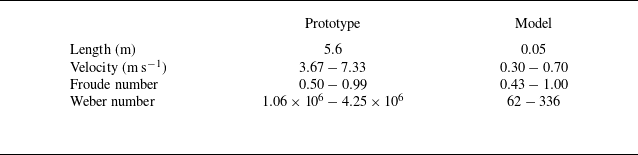
Model dimensions and velocities were scaled using Froude number similarity (table 1). The orca model had a body length of
 $41.7\,\textrm{mm}$
, tail length of
 $8.3\,\textrm{mm}$
(total length
 $L_m=50.0\,\textrm{mm}$
) and height
 $H_m$
of
 $11.1\,\textrm{mm}$
. The spanwise width (
 $W_m=55.5\,\textrm{mm}$
, five times the model height) simulated the collective width of a 4–5 orca group. At flow speeds of 0.3 to
 $0.7\,\textrm{ms}^{-1}$
, the Weber number ranged 62 to
 $336\gg 1$
; thus, surface tension effects on wave generation were neglected.
Comparison of physical parameters between the real orca and the model.

The orca model was fabricated from black photopolymer resin by three-dimensional printing. Longitudinal through-holes (
 $0.5\,\textrm{mm}$
diameter) were incorporated along the model’s spanwise direction. A
 $0.3\,\textrm{mm}$
stainless-steel wire was threaded through these internal holes and secured to
 $3.0\,\textrm{mm}$
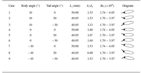
metal anchor rods mounted near the towing tank sidewalls, which connected to the overhead towing carriage. During model installation, pliers were used to tension the steel wire, and after achieving sufficient tautness, the free end was secured with an aluminium wire sleeve clamp. The pretension force in the wire effectively minimized model vibration. The above arrangement eliminated flow field disturbances from support structures as much as possible. Body pitch angle was adjusted by varying the anchor points’ relative heights on the rods, with positive angles defined by leading-edge upward tilt. Tail angle (positive when uptilted) indicated the time-averaged tap orientation during propulsion. Refer to table 2; multiple representative orca postures, from Cases 1 to 9, were systematically combined. Readers should understand that orcas do not maintain a single, specific posture throughout their swimming motion. This paper designs multiple experimental cases to test the idealized effect of a particular posture over a period of time. Such compromise and simplification are necessary when studying physical phenomena, as real-world scenarios likely involve more complex superposition or coupling of multiple states.
Parameters of orca model postures under varying body angles and tail angles.

Regardless of the installation configuration, the vertical distance
 $h$
between the dorsal high point of the orca body and the water surface was maintained
 $2H_{im}$
between the starting position (
 $P_s$
) and the termination point (
 $P_t$
). The relative submergence depth
 $h/d_y$
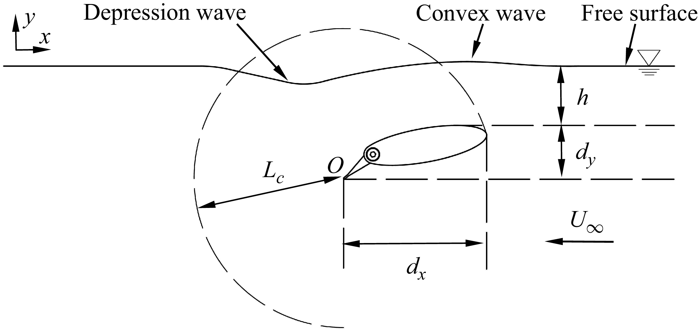
in table 2 is equally important, as it reflects the model’s gap ratio. This relative position is annotated in figure 3. The orca model features a non-axisymmetric cross-section with significant differences in the
 $x$
- and
 $y$
-directions. Therefore, two orthogonal projection distances,
 $d_x$
and
 $d_y$
, are considered to define corresponding Froude numbers,
 $\textit{Fr}_x$
and
 $\textit{Fr}_y$
. The former one is expected to influence the coupling between the wake vortex structure and the free surface, while the latter primarily governs the free surface wave pattern deformation and is directly related to the volume of fluid displaced by the body and the pressure disturbances, which propagate as gravity waves on the free surface,
 \begin{equation} \textit{Re}_c=\frac {\rho U_{\infty }L_c}{\mu }. \end{equation}
Overview of experimental arrangement and definition of flow and geometrical parameters.

Furthermore, the Reynolds number for the orca model in flow also needs to be considered. As given in (2.5) and using the chord length
 $L_c$
as the characteristic length, the Reynolds number was calculated. In the equation, the dynamic viscosity
 $\mu$
is
 $8.9\times 10^{-4}\,\textrm{Pa s}$
, and
 $L_c$
is defined as the distance between the endpoints of the tail and the head, as illustrated in figure 3. Both
 $L_c$
and
 $\textit{Re}_c$
are listed in table 2. The values confirm that the model’s motion occurs within a turbulent wake flow regime. The instantaneous streamwise (
 $x$
-axis), normal (
 $y$
-axis) and spanwise (
 $z$
-axis) velocity components at any point in the flow field are denoted as
 $u$
,
 $v$
,
 $w$
, respectively. These are composed of the superposition of the local mean velocities
 $\bar {u}$
,
 $\bar {v}$
,
 $\bar {w}$
, and their corresponding fluctuating components
 $u'$
,
 $v'$
and,
 $w'$
. The resultant velocity at a point in the flow field should be understood as the vector sum of its component velocities, i.e.
 $U=\sqrt {u^2+v^2+w^2}$
. This study mainly analyses the velocity field on the central plane of the model. Considering symmetry, the contribution of the spanwise velocity component on the centreplane of the model is neglected; therefore, the spanwise velocity component
 $w$
is scarcely discussed in this paper. Further explicit reference to the meaning of symbols will be omitted in subsequent sections.
2.2. Ice floe model
Visser et al. (Reference Visser, Smith, Bullock, Green, Carlsson and Imberti2008) reported ice-breaking widths of 4.5–18.0 m for orca groups, with maximum floe diameters reaching approximately
 $25\,\textrm{m}$
and ice thickness ranging from below
 $0.5\,\textrm{m}$
to over
 $1.5\,\textrm{m}$
. Smith et al. (Reference Smith, Siniff, Reichle and Stone1981) observed floe diameters between 5 and
 $15\,\textrm{m}$
. The dimensions and mechanical characteristics of the model ice satisfy the scaling relationship. Based on actual proportions,
 $1/5$
of the orca model length
 $L_m$
was selected as the model ice thickness
 $H_{im}\approx 10\,\textrm{mm}$
. The corresponding natural ice thickness can be estimated by the following equation:
 \begin{equation} H_{in}=H_{im}\lambda _{l}^{4/3}\left ( \left [ \sigma _u \right ] _n/\left [ \sigma _u \right ] _m \right ) ^{-1/3}, \end{equation}
where
 $H_{in}$
and
 $H_{im}$
represent the thicknesses of natural ice and model ice, and
 $ [ \sigma _u ] _n$
and
 $ [ \sigma _u ] _m$
denote the flexural strengths of natural ice and model ice, respectively. Using the upper limit of sea ice flexural strength reported by Timco & O’.Brien (Reference Timco and O’.Brien1994) as the reference value (
 $ [ \sigma _u ] _n\approx 1.50\,\textrm{MPa}$
), the flexural strength of the model ice was designed as
 $ [ \sigma _u ] _m\approx 9.53\,\textrm{kPa}$
to simulate natural ice thickness
 $H_{in}\approx 1/5L_o$
.
As shown in figure 2(b), the ice floe substrate was fabricated using polystyrene foam boards cut into
 $10\,\textrm{mm}$
-side-length regular hexagonal units (density of
 $0.42\,\textrm{gcm}^{-3}$
) to simulate columnar ice cross-sections. Waterproof silicone adhesive was applied to bond hexagonal aluminium plates (density of
 $2.80\,\textrm{gcm}^{-3}$
) of identical dimensions atop the foam units. When the aluminium plate thickness was
 $1/5H_{im}$
and the foam thickness
 $4/5H_{im}$
, the model ice density reached
 $0.90\,\textrm{gcm}^{-3}$
, which approximates real ice conditions (Dumont, Kohout & Bertino Reference Dumont, Kohout and Bertino2011), with approximately
 $1/10$
of its height exposed above water (Squire Reference Squire2011).
One of the reviewers astutely pointed out that using non-uniform materials to fabricate the ice model may lead to an upward shift in the centre of mass of the ice units, which could potentially affect the motion and stress response of the ice under dynamic conditions. We note that when the ice floe model consists of multiple interconnected units, the larger ice structure can be regarded as an integrated whole. In such a case, the potential influence of centre-of-mass variation may be mitigated. Furthermore, independent motion of numerous uncontrolled small ice floe units seldom occurs in the subsequent analysis, which allows us to maintain a degree of tolerance regarding the shift in the centre of mass. It is important to remind the reader that even in natural sea ice, density varies vertically. From this perspective, even homogeneous materials would also fall short in accurately simulating real ice floes.
The large continuous ice floe model was assembled from small hexagonal ice units bonded with
 $\alpha$
-cyanoacrylate adhesive. The adhesive is dot-applied to the side of an aluminium plate using a metal rod with a diameter of 1 mm. The plate is then brought into contact with the aluminium plate side of an adjacent ice unit and rapidly clamped for curing. As shown in figure 2(c), the large continuous ice floe model consisted of 44 units arranged in three columns: the first and third columns each consisted of 15 units, while the middle column contained 14 units. We also fabricated a discrete model, where individual ice units maintained gaps of approximately 1 mm and were interconnected with cotton threads. This discrete configuration was designed to simulate small ice floe groups consisting of fragmented but closely spaced floating ice pieces. It should be noted that the slender layout ignores the three-dimensional effects to some extent.
Figure 2(d) illustrates that the equivalent flexural strength between bonded units was estimated via three-point bending tests (Timco & O’.Brien Reference Timco and O’.Brien1994), with loading applied parallel to adhesive seams at a constant rate. The flexural strength is expressed as
 \begin{equation} \sigma _f=\frac {3Pl}{2bH_{im}^{2}}, \end{equation}
where
 $P$
is the applied load,
 $l=40\,\textrm{mm}$
denotes the support span of the ice floe beam and
 $b=H_{im}=10\,\textrm{mm}$
represents the width and height of the ice floe beam, respectively. As shown in figure 2(e), six independent measurements of the flexural strength of the ice floe beam were conducted. The mean results demonstrated that the beam exhibited linear deformation under loading until fracture occurred at displacements exceeding
 $0.06\,\textrm{mm}$
, with a maximum recorded load of approximately
 $0.33\,\textrm{N}$
. While initial deformation stages exhibited excellent reproducibility, displacement-dependent divergence emerged, likely due to differences in
 $\alpha$
-cyanoacrylate wetting and curing. The derived flexural strength at peak load was
 $\sigma _f\approx 19.80\,\textrm{kPa}\gt [ \sigma _u ] _m$
. Notably, flexural strength parameters of the natural sea ice display inherent variability influenced by hydrographic conditions, brine volume, ice temperature and loading rate (Han et al. Reference Han, Jia, Huang and Li2016). Elevated temperature or brine content reduces strength, with young ice exhibiting higher strength than aged ice (Fransson Reference Fransson2002). Reported sea ice flexural strengths range 0.1–1.5 MPa (Timco & O’.Brien Reference Timco and O’.Brien1994). The artificial ice floe models in this study may simulate thicker ice than intended (i.e. ice floe with a thickness of
 $1.27\,\textrm{m}$
), though all values remain within physically plausible ranges.
Panels (a) and (b) illustrate the parameter configurations for experiments on wave-induced overturning of large and small continuous ice floe models. Panels (c), (d) and (e) present the parameter configurations for experiments measuring the three-dimensional microforce response of an ice floe unit under wave action. In (c), only the force on the isolated ice floe unit is measured. In (d) and (e), continuous and discrete ice floe models are placed upstream of the target unit. In all experiments, the ice floe unit, ice floe models and orca model must be aligned on the same central plane. During preparation, the water surface must remain calm, and the positions of the ice floes must be carefully adjusted.

In all experiments presented in this study, the leading edge of the ice floe model was positioned
 $550\,\textrm{mm}$
downstream in the towing tank. Figures 4(a) and 4(b) illustrate the experimental set-ups for investigating wave-induced tilting effects on large continuous ice floes (arranged in a
 $15\times 14\times 15$
array) and small continuous ice floes (arranged in a
 $5\times 4\times 5$
array). High-speed cameras were employed to capture snapshots of the ice floe overturning process. Figure 4(c) depicts the force measurement set-up for waves acting on an isolated ice floe unit (positioned
 $850\,\textrm{mm}$
downstream in the towing tank). In configurations figure 4(
d) and figure 4(
e), modifications were made by placing continuous and discrete large ice floes upstream of the target unit to evaluate the dissipation effect of different ice floe arrays on subsequent wave forces. A custom-designed force balance was used for force measurements. Further details regarding the high-speed camera and the force balance are provided in subsequent sections. Please note, the edge of the upstream water surface in the towing tank is regarded as the geometric origin for describing key locations in the side view, refer to figure 2(h).
2.3. Towing tank and flow field visualization system
The experiments were conducted in the wind tunnel laboratory at the School of Mechanical Engineering, Northwestern Polytechnical University. Given the significant difference in viscosity between air and water at room temperature, the influence of air on the water flow is neglected to approximate the conditions of a free surface. As illustrated in figure 2(f), all towing experiments were conducted in a custom-built transparent acrylic water tank with internal dimensions of
 $L_t=24.0L_m$
(length,
 $x$
-axis),
 $W_t=9.1W_m$
(width,
 $z$
-axis) and
 $H_t=32.4H_m$
(depth,
 $y$
-axis). Under these parameters, sidewall effects on wave generation were negligible, and deep-water conditions were satisfied.
Two 1200-mm-long linear metal rails were installed along the tank sides. A towing carriage, constructed from 2020 aluminium profiles with redundant structural reinforcement, was mounted on the rail sliders. The carriage featured dual rod holders, each securing two 3-mm-diameter, 550-mm-long stainless-steel rods positioned approximately 30 mm from the sidewalls, perpendicular to the water surface. Calibrated anchor points on the rods enabled model pitch adjustment. The carriage was towed via steel cables driven by a stepper motor at the tank end. Towing speed was calibrated using high-speed imagery and scale markers. A light-emitting diode (LED) panel was mounted atop the carriage and modified to display 10 mm black/white zebra stripes. A smartphone, fixed via a customized holder (orange one in the upper-right-hand inset), recorded reflected patterns at 4K/60 f.p.s. to quantify free-surface deformation and corresponding wake scars and striations (
 $3840\times 2160$
pixels). The smartphone position was adjusted to maximize pattern coverage. Beside the towing carriage, a high-speed camera (Cyclone-2–2000 M, Optronics; lens: AF-S Nikkor 24–120 mm f/4 ED VR, Nikon) was mounted laterally on a platform to capture horizontal free-surface snapshots (
 $1920\times 1080$
pixels) at the model centreplane and the total field of view is approximately
 $220\,\textrm{mm}\times 70\,\textrm{mm}$
(
 $x \times y$
). The camera sampling rate is set to 250 Hz.
For particle image velocimetry (PIV), the LED panel was replaced with a 7.5 W maximum power continuous laser (532 nm, 5W-EC31811, Changchun New Industries Optoelectronics Tech. Co., Ltd.) generating a 0.5-mm-thick light sheet (
 $30^\circ$
divergence angle) aligned with the orca model’s centreplane (see bottom-left-hand inset of figure 2
f). A black velvet cloth was attached to the outer surface of the acrylic water tank wall opposite the high-speed camera to improve image quality and reduce unwanted laser reflections. Due to the mechanical structure of the support frame, the laser sheet was incident on the water surface from the top. The refraction from the deformed free surface introduced minor perturbations to the instantaneous velocity field at the wake interface, where vortex structures frequently impinged. However, the averaged results demonstrated a convergent trend, but it is still recommended that future studies employ a bottom-incident laser sheet. The rod holder of the towing carriage caused a minor obstruction in the PIV sampling area, potentially introducing errors in cross-correlation calculations near the obscured edges. Nevertheless, these regions were readily identifiable and did not affect the conclusions of this study. The water was seeded with
 $50\,\unicode {x03BC}\textrm{m}$
polyamide resin particles (refractive index, 1.56; density,
 $1.03\,\textrm{g}\,\textrm{cm}^{-3}$
), and the camera was repositioned horizontally relative to the model. The sampling rate of the high-speed camera needed to be reconfigured and increased to 2000 Hz to avoid particle streaking effects. The PIV data were processed using the PIVLab software package (version 3.06). A final interrogation window of
 $8 \times 8$
pixels with 50 % overlap was used to satisfy the Nyquist criterion. Instantaneous and ensemble averaging of velocity vectors was conducted via cross-correlation. The time-averaged quantities were obtained from 500 frames of the instantaneous velocity field. All imaging stations were positioned within the fully developed flow region, approximately 700 mm downstream of the towing tank.
A three-dimensional microforce balance was positioned externally downstream of the towing tank. To isolate the measurement system from vibrations induced by towing dynamics, the force balance was mounted on an independent vibration-damping support. The balance’s sensing probe was fitted with an ice floe unit through a carbon-fibre rod, positioned 850 mm downstream of the towing tank edge. The limit switch installed beside the rail ensured consistent travel (between
 $P_s$
= 150 mm and
 $P_t$
= 950 mm from the upstream edge), with the orca model having fully cleared the ice structures before motor deceleration was triggered. Additional tank details are provided in figure 2(h).
2.4. Decoupling-free balance for three-dimensional microforce measurement
Figure 2(g) shows a custom-designed decoupling-free three-dimensional microforce balance that was used to measure the micromechanical responses of an isolated ice floe unit under wave action. The ice floe unit was fixed to the end of a 3-mm-diameter carbon-fibre rod, which was clamped to the front end of the balance’s measuring probe (configured as a cantilever-beam lever). When hydrodynamic forces act on the ice floe unit, the force signals are transmitted through the cantilever beam to the balance for measurement.
The balance operates on an air-floating principle, with its core component being an independently designed two degrees-of-freedom (DOF) air-bearing platform. The mechanical structure was inspired by the one-dimensional air bearing proposed by Zhou et al. (Reference Zhou, Liu, Sun, Lyu, He and Yuan2025). When high-pressure gas is supplied, the air bearing achieves gas lubrication, reducing the frictional resistance of moving parts to negligible levels. The two-DOF air bearing provides predecoupled force measurement in the horizontal
 $x$
-
 $z$
plane. The forces are calculated by measuring the microdisplacements of the air-bearing slider in orthogonal directions within the horizontal plane, combined with the stiffness coefficients of elastic elements. The
 $y$
-axis force is measured using a stress–strain sensor, with the lever structure enhancing force measurement resolution. The moving components of the balance are free from interference by external cables or mechanical structures, enabling pure three-dimensional microforce measurements. The stiffness coefficients of the balance in the
 $x$
- and
 $z$
-axes are
 $23.451\,\textrm{N}\,\textrm{m}^{-1}$
and
 $25.458\,\textrm{N}\,\textrm{m}^{-1}$
, respectively. Given the use of an infrared laser sensor with
 $0.5\,\unicode {x03BC}\textrm{m}$
resolution to measure microdisplacements, the force resolutions in these directions are approximately
 $1.17\times 10^{-5}\,\textrm{N}$
and
 $1.27\times 10^{-5}\,\textrm{N}$
, with measurement ranges of
 $\pm 0.31\,\textrm{N}$
and
 $\pm 0.19\,\textrm{N}$
, respectively. The combined uncertainties in each direction arise from the laser sensor and elastic elements, resulting in relatively expanded uncertainties of 0.68 % and 0.33 % for the
 $x$
- and
 $z$
-axes, respectively.
For the
 $y$
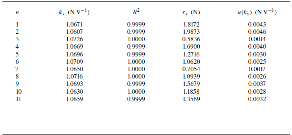
-axis, the cantilever beam was modified with an extended length, and the position of the stress–strain sensor was altered, necessitating recalibration. The calibration procedure and results are provided in Appendix A. The stiffness coefficient in
 $y$
-axis is
 $1.0671\,\textrm{NV}^{-1}$
, with a resolution of approximately
 $1.07\times 10^{-4}\,\textrm{N}$
and a measurement range of
 $\pm 0.6\,\textrm{N}$
. The uncertainty of the stiffness coefficient is approximately
 $0.001\,\textrm{NV}^{-1}$
, corresponding to a relative uncertainty of 0.1 %. The balance operates at a sampling rate of 10 Hz, with triaxial force signals transmitted to a microprocessor via LoRa wireless protocol before being collectively relayed to a computer. Testing confirmed that the system’s clock drift remains below
 $10\,\textrm{ms}$
over 20-min operation periods, which indicates that the influence of sampling circuitry on measurement results was negligible. For additional technical details regarding the balance, refer to the work by Zhou et al. (Reference Zhou, Huang, He and Yuan2026).
The free surface deformations under different cases and towing speeds. The background grid is solely used for evaluating surface deformation and is not associated with a specific reference position.

3. Results
3.1. Free-surface depression wave
Figure 5 presents the wave patterns on the vertical central plane of the model for Cases 1 to 9 under towing speeds of 0.3 to
 $0.7\,\textrm{m}\,\textrm{s}^{-1}$
. The contour points were obtained from the averaged statistical results of multiple stacked image frames. Spline curves defined by control vertices were used to connect the contour points, which were then plotted on a grid. This process temporarily neglected small-scale fluctuations of the liquid surface, thereby illustrating the macroscopic deformation of the free surface. Distinct differences in wave patterns are observed among the cases, with both the body and tail parts of the orca model influencing wave development.
Cases 1 to 3 all produced readily identifiable depression waves. The depression wave in this article specifically refers to the first trough appearing behind the model. The depression wave in Case 3 was the most pronounced, reaching a depth of 22.8 mm at
 $0.7\,\textrm{m}\,\textrm{s}^{-1}$
, followed by Case 1, which generated a depression wave of
 $15.9\,\textrm{mm}$
at the same speed – the former being approximately 1.4 times deeper than the latter. The streamwise positions of the wave troughs (with the leading edge of the orca model’s head as the origin) were
 $86.6\,\textrm{mm}$
downstream for Case 3 and
 $81.3\,\textrm{mm}$
downstream for Case 1. However, when the model’s tail was uptilted (Cases 2, 5 and 8), the depression wave was significantly suppressed, affecting both the trough depth and its streamwise position. In Case 2, the maximum trough depth was only
 $7.2\,\textrm{mm}$
, located at
 $74.1\,\textrm{mm}$
downstream, under a towing speed of
 $0.7\,\textrm{m}\,\textrm{s}^{-1}$
.
In Cases 4 to 6 and 7 to 9, downward flipping of the tail resulted in more pronounced tail depression waves. Conversely, uptilting the tail suppressed the depression wave. Intergroup comparisons indicate that the wave depth and streamwise position in these cases are all smaller than those in Cases 1 to 3. Additionally, localized elevations of the liquid surface above the undisturbed free surface were observed in Cases 5 and 8, to the extent that in Case 8, the depression wave even rose above the free surface. This is often attributed to a locally increased Froude number above the model, where exceeding a critical value can induce a hydraulic jump. This Froude number is determined by the local velocity
 $U$
and local liquid height
 $h_l$
, i.e.
 $\textit{Fr}_l=U/\sqrt {gh_l}$
, which will be further explained later. More broadly, the depression wave depths in Cases 5, 7 and 8 were all relatively small, with troughs close to the free surface, and uptilted tails were a common feature among these three cases.
Panels (a) and (b) show the positional data of the head wave crest and stern wave trough under different cases and towing speeds, respectively. Panels (c) and (d) present the corresponding data normalized using
 $d_y$
and
 $d_x$
for the peak and trough points. Here ‘
 $-$
’ indicates being below the calm surface or downstream of the leading-edge reference point of the model. The colour of the symbols in the figure represents different towing speeds, consistent with figure 5.

The convex wave generated at the model’s head also attracts attention, primarily influenced by the blockage effect at the model’s frontal stagnation point. The height of the convex wave is related to both
 $h/d_y$
and the towing posture. Most convex wave peaks are located 10 to
 $20\,\textrm{mm}$
downstream of the model’s leading edge. Case 8, with the smallest gap ratio (
 $h/d_y=0.88$
), produced the most prominent convex wave, reaching a peak height of
 $13.1\,\textrm{mm}$
at
 $0.7\,\textrm{m}\,\textrm{s}^{-1}$
, situated
 $44.1\,\textrm{mm}$
downstream of the head. In contrast, the wave heights in other cases were relatively moderate. Cases 1 and 3 exhibited the least sensitivity to convex wave generation, with minimal variation in wave height with towing speed and limited streamwise displacement. As towing speed increased, the downstream shifting of the convex wave slowed. An upward tilt of the head mitigated the blockage effect, thereby suppressing the growth of the convex wave. Cases 5, 7, 8 and 9 showed relatively larger streamwise displacement ranges of the convex wave. Among these, Case 5 featured an uptilted tail, while Cases 7 to 9 involved a downward pitching of the body. Their common feature is the deflection of the dorsal flow towards the water surface, which contrasts sharply with Cases 1 and 3. Figures 6(a) and 6(b) present the parameter distributions of the trough behind the model and the convex wave peak, respectively, with the gap ratio annotated in figure 6(
a) for reference.
Figures 6(c) and 6(d) present the normalized wave trough and peak positions in the normal direction and the streamwise position. In figure 6(c), the peak points exhibit a more uniform distribution pattern. All data points lie below a straight line with a slope of
 $-8/17$
, showing a compact distribution. The slope reflects the trend of the peak position variation with towing speed. The physical significance of this line lies in the constraint imposed by the orca’s attitude on the convex wave peak, indicating that a higher convex wave peak cannot form farther upstream. This relationship satisfies
 \begin{equation} \frac {y}{d_y}\lt -\frac {8}{17}\frac {x}{d_x}+\frac {28}{85}. \end{equation}
Cases 1, 3 and 9 lie at the lower-left-hand outermost side of the line, indicating that these three cases exhibit stronger suppression of the convex wave compared with most other conditions. Similarly, in figure 6(d), only the curves of Cases 1, 3 and 6 continue to show a proactive downward trend in the lower left-hand corner, as indicated by the grey arrow. In these plots, a redder background colour corresponds to a more significant depression wave; thus, movement towards the lower left-hand region represents a deepening of the depression wave. All these cases share a common configuration: a downward-oriented tail.
Optical path diagram of zebra stripes on the LED panel reflected by the wave surface. The coloured arrow above reflects the movement trend of the projection points in the camera. The slope
 $k_w$
of the line connecting the wave crests and wave troughs in the figure is used to evaluate the depression degree of the waves. The figure is not drawn strictly to scale.

In this study, the LED panel and smartphone lens were fixed relative to the towing carriage to capture the images of the surface deformation during the towing process. Before focusing on results, it is necessary to clarify the influence of wave peak and trough on the reflective stripes. Figure 7 illustrates a simplified two-dimensional relationship among the camera, LED panel, waves and optical path. Although the elements are not drawn strictly to scale, the diagram is sufficient for explanatory purposes. Ten equally spaced reflection points
 $r_i$
(
 $i=1- 10$
) were selected on the deformed surface. The reflected light paths from these points to the camera were constructed, and their intersections with the plane of the LED panel are denoted as corresponding projection points
 $p_i$
(
 $i=1- 10$
). The coloured arrows above the figure, matching the light paths, indicate the positional variations of these projection points. The stretch ratio of the zebra stripes is defined as

where
 $\eta _i$
reflects the average stretch ratio between points
 $p_i$
and
 $p_{i+1}$
. Evidently,
 $\lim _{p_i\rightarrow p_{i+1}} \eta _i$
can represent the local stretch ratio. Considering that
 $p_i$
may exhibit turning points at
 $t_1$
and
 $t_2$
, ‘
 $\rightarrow$
’ is used here to distinguish the displacement between these two points from the conventional arclength. When
 $\eta _i$
is greater than unity, the pattern on the free surface is compressed, resulting in denser stripes; conversely, it is stretched when
 $\eta _i$
is less than unity. The degree of compression or stretching is related to the magnitude of
 $\eta _i$
.
Zebra stripe patterns for Cases 1 to 3.

For the reflection points in figure 7,
 $\eta _1$
at
 $p_1$
(convex wave) reaches its maximum and decreases during the transition from
 $p_1\rightarrow p_3$
. The stripes are most densely concentrated over the head wave peak. Near
 $p_3$
, a topological change in the stripes begins (i.e. the inverse process at
 $t_1\rightarrow t_2$
), accompanied by a thickening of the stripes. When a gradient in curvature exists along the spanwise direction (typically with curvature decreasing away from the deformation core on both sides), the LED panel stripes reflected from the central plane of the model generally appear farther downstream. Thus, the topological pattern manifests as concentric rings. The projection points
 $p_3\rightarrow p_7$
, corresponding to reflection points
 $r_3\rightarrow r_7$
, reverse direction and point upstream until the end of
 $t_2$
in the arrow diagram. Thereafter, projection points beyond
 $r_7$
(
 $p_7\rightarrow p_{10}$
) consistently move downstream, indicating that only regions downstream of
 $r_7$
in the camera view will exhibit reflective stripes with non-topological and conventional distribution.
Zebra stripe patterns for Cases 4 to 6.

Observing
 $p_3$
to
 $p_7$
, one can find
 $\eta _5=Max\{ \eta _3,\eta _4,\eta _5,\eta _6\}$
. The compressive effect can be used to identify the location of the trough at
 $r_5$
, where the stripes are locally most dense and close to the downstream position of the first topological concentric ring. Similarly, the decrease in stretch ratio as the projection points move towards
 $p_{10}$
implies gradually widening stripes near the wake wave peak. It should be noted that the turning point
 $t_2$
in figure 7 lies outside the LED panel, indicating possible discontinuities between upstream and downstream stripes. This phenomenon is related to the curvature of the wave trough. If the depression at
 $r_5$
is shallow and the range of
 is small enough such that t
2 falls within the LED panel, the stripe pattern remains continuous despite the topological transition. Based on the principles described above, the approximate extent and peak location of the convex wave are indicated by red dashed lines and arrows. The approximate starting boundary and trough of the depression wave are marked with blue dashed lines and arrows. The approximate peak location of the wake convex wave is indicated by magenta arrows. The absence of any annotation implies that no valid physical information can be identified.
Zebra stripe patterns for Cases 7 to 9. The dark fringes indicated by the green arrows are traces of the model tip vortices striking the water surface (Zhang et al. Reference Zhang, Hayostek, Amitay, He, Theofilis and Taira2020).

Figures 8 to 10 provide further information on the free surface deformation through zebra-stripe patterns. For an overview of the reflective pattern method used to measure free surface deformation, refer to the review by Gomit, Chatellier & David (Reference Gomit, Chatellier and David2022). A small convex bulge typically forms above the model, while a concave bow wave develops at the model’s stern, representing a specific derivative of Kelvin wave patterns under the given operational conditions (Xue et al. Reference Xue, Jin, Qiu and Yang2020). At low towing speeds (
 ${\lt } 0.4$
to
 $0.5\,\textrm{ms}^{-1}$
), capillary waves are observed on the upward slope plane downstream of the trough (within the yellow dashed box). The wavelength of capillary waves decreases towards the centre of the wave trough, where they are densely packed, while the wavelength gradually increases towards the outer flanks. The waves fan outward, and this spanwise variation arises from differences in the crest velocity and trough velocity of the capillary waves in the spanwise direction (Duncan et al. Reference Duncan, Qiao, Philomin and Wenz1999). Outside the capillary wave region, the surface generally remains calm, except for faint vortex impingement traces immediately downstream of the depression wave – specifically in the region of maximum surface curvature – where a locally sharpened fine annular topological pattern emerges. As the towing speed increases continuously, this local vorticity rapidly diffuses and destabilizes, evolving into large-scale breaking waves that cover the entire area enclosed by the Kelvin wave pattern. A key transition occurs when the towing speed increases beyond a certain threshold (approximately
 $0.5$
to
 $0.6\,\textrm{ms}^{-1}$
): the capillary waves disappear. At this point, the vorticity near the interface downstream of the trough undergoes a complete transformation, leading to a flow state dominated either by large-scale vortices or a smooth, steady interface. According to the study of Longuet-Higgins (Reference Longuet-Higgins1992), the initial stage of short gravity wave breaking involves the appearance of parasitic capillaries. As the Reynolds number increases further, gravity induces a natural downward sliding of the interface along the sloped water surface behind the trough (Duncan et al. Reference Duncan, Philomin, Behres and Kimmel1994). This sliding fluid impacts the leeward face of the wave; the intervening fluid is continuously entrained, forming a shear layer. Separation from the underlying fluid triggers a turbulent state, leading to the formation of a capillary roller (Longuet-Higgins Reference Longuet-Higgins1992). Dimas & Triantafyllou (Reference Dimas and Triantafyllou1994) indicated that intense horizontal shear is the primary trigger for small, sharp surface waves near the free surface at low Froude numbers. Interestingly, the capillary waves were absent at the lowest Reynolds number in Case 5. Observation of figure 5 reveals that the trough depth for Case 5 is shallow. A flatter wave surface is less prone to breaking at the interface. Deike, Popinet & Melville (Reference Deike, Popinet and Melville2015) previously noted that waves with low initial steepness remain stable, propagating smoothly without breaking. When the trough steepness is small, capillary waves induce only localized interfacial vorticity near the trough.
Distribution of wake types under different
 $k_w$
and towing speeds, where Type 1–4 wakes are represented by green, yellow, blue and red, respectively.

Typically, vortices shed from the orca stern impinge on the water surface downstream of the wave trough (downstream of the blue arrow). However, in Case 8, vortex impingement is observed upstream of the capillary wave. Figure 10 presents snapshots of the interfacial vortex structures for Case 8 at different Reynolds numbers. At the lowest Reynolds number, evidence of large-scale vortex impingement is observed at the upstream trough location relative to the capillary waves, while the area downstream of the capillary waves shows dense, small striations formed by the impingement of small-scale, high-frequency waves. When the Reynolds number increases to 28 383, the impingement of large-scale structures even makes the wave trough difficult to discern. As the Reynolds number increases further, the wake becomes dominated by large-scale structures and the capillary waves disappear gradually. The upward transport tendency of Case 8 is highly evident, as it even convects the tip vortices from both sides of the model to the vicinity of the interface, where their impingement on the free surface leaves visible ‘traces’, as indicated by the green arrows in the figure. The development path of vortices downstream of an irregular cross-section body is closely related to its attitude (Subburaj, Khandelwal & Vengadesan Reference Subburaj, Khandelwal and Vengadesan2018), a point that will be discussed in § 3.2 regarding the underwater flow structures. The subsequent part of this section continues to focus on the characteristics of vortex impingement on the interface.
Based on the morphological differences of the impinging vortices, the model wake is categorized into four types. Type 1 features small-scale shedding vortex structures that cause small-range vortex impingement on the surface. The diameter of a single vortex is much less than
 $W_m$
. These vortices shed from the wave trough and collide with the deformed surface, with an emergence width of 1 to several times the diameter of the impact vortex, which subsequently diminishes or vanishes as they follow the wake. Type 2 involves wide-range small-scale vortex structures. When the Reynolds number further increases based on the Type 1 wake, shortly after the formation of the depression, the wake instantly transitions into a large-area ‘orange peel’ pattern covering the entire downstream region of the depressed wave that induces large-area intensive fluctuations in the wake region. The initial width is significantly larger than
 $W_m$
, and its extent is confined within the band-like depression region (the region downstream delineated by capillary waves). The vortex impingement frequency is higher than in Type 1. Individual vortex sizes are at the level of Type 1 and are distributed very densely. Type 3 forms a steady wake region where the surface is smooth, the streak spacing is highly regular, and the curvature variation is small. No action between the shedding vortices and the liquid surface is observed. This scenario typically occurs in cases with deeper tail depression waves. Type 4 involves large-scale shedding vortex structures, where the size of a single vortex is often comparable to
 $W_m$
. These structures gradually enlarge while developing downstream. Adjacent vortex structures usually appear sequentially without clustering, which may be related to the spanwise asymmetry of the vortex structures. The study showed that this characteristic is one cause of the aperiodic nature of vortex shedding and is a feature of wakes behind finite-aspect-ratio models, with asymmetric flows more prone to occur at higher Reynolds numbers (Taira & Colonius Reference Taira and Colonius2009). In figures 8 to 10, a slash bar ‘
 $\diagdown$
’ added to an arrow indicates small-scale vortex structures, a wavy line ‘
 ${\sim}$
’ denotes large-scale vortex structures and the absence of a symbol represents steady flow. If an arrow lacks an annotation, it implies that the flow feature at that location is difficult to identify, for instance, if it is outside the field of view.
Deike et al. (Reference Deike, Popinet and Melville2015) indicated that the Bond number and the initial wave steepness can be used to classify wave regimes, as surface tension significantly influences interfacial wave development. We propose that the wake type is associated with both the Reynolds number and the steepness of the wave concavity. We have plotted the wake type, Reynolds number and the downslope steepness
 $k_w$
(defined in figure 7) in a single diagram. When the wave depression is limited and the towing speed is low, Type 1 wake dominates and is distributed in Area 1. Capillary waves downstream of the wave trough are typically observed in this regime. Case 8 unexpectedly appears in this region because its attitude forcibly guides the trailing vortices towards the surface. As
 $k_w$
increases, the wake transitions from Type 1 to Type 2. The spatial extent of Type 2 wake is considerably larger than that of Type 1, and their underlying formation mechanisms differ. The steeper slope promotes the formation of a jet beneath the trough and a large-area shear layer near the free surface, generating numerous surface vortices. Lin & Rockwell (Reference Lin and Rockwell1995) investigated wave breaking phenomena downstream of a hydrofoil and observed that with increasing Froude number, capillary waves are replaced by large-scale free-surface distortions, which are induced by flow separation near the free surface at the wave trough where the curvature is large. Figure 12 illustrates the interface sharpening near the wave trough at lower Reynolds numbers, where capillary waves typically appear on the upward slope behind the trough. As the flow velocity increases, the sharpened trough becomes more prone to intense flow separation. When both the depression depth and the velocity are relatively high, the wake transitions from Type 2 to Type 3. In this case, the capillary waves behind the trough disappear, and severe curvature variations on the interface are significantly reduced. The free surface in Type 3 is smooth, indicating a steady flow state, and no vortex impingement is observed within the camera’s field of view. It is worth noting that Type 3 may require a specific deeper wave trough. In most cases where a sufficiently deep concave wave cannot be formed, the wake exhibits patterns left by the impingement of large-scale vortices, that is, the Type 4 wake. We tend to believe that Type 3 and Type 4 are essentially the same underwater flow pattern, i.e. Strouhal vortex shedding state, with the distinction lying in whether the large-scale wake vortices are convected to shallower surface-sensitive regions.
A snapshot of the deformed water surface for Case 3 at a towing speed of
 $0.3\,\textrm{m}\,\textrm{s}^{-1}$
.

In this paper, the initial state of the liquid surface corresponds to Type 1. As the wave trough deepens and its curvature increases, flow shear instability beneath the trough triggers a transition to Type 2. With a further rise in the Reynolds number, capillary waves disappear, and stable flow at the trough replaces flow separation. If the wake intensity is high or its position is close to the water surface, the large-scale vortex structures will reach the interface, leading to a transition to Type 4. Conversely, if the wake intensity is weak or is guided by the model to deeper layers, it becomes insufficient to affect the interface, resulting in a transition to Type 3. The absence of capillary waves serves as a critical indicator of the transition from Type 1/2 to Type 3/4, corresponding to a Reynolds number range of 28 000–29 000.
At low Froude numbers, the free surface can stabilize the flow field, while high Froude numbers typically induce large-amplitude waves. The Froude number is closely related to the stability of the downstream wake (Triantafyllou & Dimas Reference Triantafyllou and Dimas1989). Some studies indicated that at low Froude numbers, the interaction between vortices and the free surface resembles that with a rigid surface, whereas at high Froude numbers, significant deformations occur (Yu & Tryggvason Reference Yu and Tryggvason1990; Tryggvason et al. Reference Tryggvason, Unverdi, Song and Abdollahi-Alibeik1991). Although free-surface deformations induced by near-surface cylinders have been extensively studied (Sheridan et al. Reference Sheridan, Lin and Rockwell1995, Reference Sheridan, Lin and Rockwell1997; Reichl, Hourigan & Thompson Reference Reichl, Hourigan and Thompson2005; Sun et al. Reference Sun, Lu, Patel, Zhu and Yang2025), the Froude number for a cylinder is determined solely by its diameter. In contrast, the present model involves two distinct Froude numbers: the streamwise Froude number
 $\textit{Fr}_x$
and the normal Froude number
 $\textit{Fr}_y$
. The dimensionless depth and streamwise position of the trough of the depression wave are plotted against the corresponding directional Froude numbers in figure 13. For all cases, as
 $\textit{Fr}_x$
and
 $\textit{Fr}_y$
increase, the wave trough moves farther away from the orca model. However, the depth of the trough is influenced by the model’s attitude. Several differences are noteworthy. Regarding the streamwise position
 $x/d_x$
, the trough in Cases 1 to 3 remains closer to the model, with a moderate rate of change as
 $\textit{Fr}_x$
increases. In contrast, Cases 7 to 9 exhibit a more pronounced downstream shift with increasing
 $\textit{Fr}_x$
. Although data for Case 8 is incomplete, its trend suggests a substantial displacement. Based on the results in figure 5, it can be anticipated that the trough will appear farther downstream. In comparison, Cases 4 to 6 show lower sensitivity to
 $\textit{Fr}_x$
, with
 $x/d_x$
being the least responsive to changes in
 $\textit{Fr}_x$
.
Variation of the dimensionless streamwise location and depth of the wave trough with Froude number
 $\textit{Fr}_x$
and
 $\textit{Fr}_y$
, respectively.

Regarding the dimensionless trough depth
 $y/d_y$
, Cases 1 and 3 show a rapid deepening of the trough with increasing
 $\textit{Fr}_y$
, resulting in significant depression waves at high Froude numbers. Case 6 exhibits a similar trend but at a reduced rate. The remaining cases show minimal change in
 $y/d_y$
with increasing
 $\textit{Fr}_y$
. For complex models, the trend of free surface variation cannot be evaluated solely by the Froude number, as the contribution of the geometry of the flow-disturbing cross-section may be comparable to that of the Froude number. The study by Daichin & Lee (Reference Lee2004) indicated that even for elliptical cylinders with aspect ratios of 3–4, the influence of surface curvature on free surface deformation and wake flow structure exceeds that of the Froude number. Given the greater complexity of the model in this study, the influence of the Froude number is likely to be less significant than in traditional bluff bodies. The interaction mechanism between the vortex structures behind the orca model and the free surface is complex and requires further analysis of the flow field below the water surface.
3.2. Flow field below the water surface
When towed beneath the free surface, the model satisfies both asymmetric boundary conditions and asymmetric geometric conditions (Inoue & Sakuragi Reference Inoue and Sakuragi2008; Subburaj et al. Reference Subburaj, Khandelwal and Vengadesan2018; Samsam-Khayani & Seyed-Aghazadeh Reference Samsam-Khayani and Seyed-Aghazadeh2025). The asymmetric boundary conditions arise from the combined effects of the geometry and the free surface. Unlike the periodic wake patterns typically observed under symmetric boundary conditions, the wake flow structure of the orca model is expected to undergo significant alterations due to additional constraints (Taneda Reference Taneda1965; Alzabari, Wilson & Ouro Reference Alzabari, Wilson and Ouro2023). The asymmetric wake induced by the angle of attack was initially investigated by Fage & Johansen (Reference Fage and Johansen1927). Primary focus is often placed on boundary layer development, subsequent shear layer instability, and the separation of leading- and trailing-edge vortices, phenomena that have been extensively analysed in studies of flow around flat plates (Perry & Steiner Reference Perry and Steiner1987; Nakamura, Ohya & Tsuruta Reference Nakamura, Ohya and Tsuruta1991; Samsam-Khayani & Seyed-Aghazadeh Reference Samsam-Khayani and Seyed-Aghazadeh2025). This section examines the flow dynamics around the orca model in different attitudes using time-averaged velocity fields, time-averaged vorticity fields, time-averaged swirling strength vector fields, instantaneous vorticity and streamlines.
The dimensionless vorticity
 $\omega _{z,n}$
is obtained by normalizing the vorticity
 $\omega _z=\partial v/\partial x-\partial u/\partial y$
using the chord length
 $c$
and the towing speed
 $U_{\infty }$
,
 \begin{equation} \omega _{z,n}=\frac {\omega _zc}{U_{\infty }}. \end{equation}
The time-averaged dimensionless vorticity
 $\langle \omega _{z,n} \rangle$
characterizes the average distribution of vorticity over time in the wake of the model. The coherent-structure identification criterion based on
 $\boldsymbol{\lambda }_{ci}$
is employed to detect and characterize vortex structures in complex flow fields. This method is grounded in the concept of swirling strength and involves analysing the eigenvalues of the velocity gradient tensor
 $\boldsymbol{eig} ( \boldsymbol{\nabla }\boldsymbol{u} )$
. Regions with enhanced vortex activity are identified by the presence of a complex eigenvalue pair, with higher
 $\boldsymbol{\lambda }_{ci}$
values indicating stronger swirling motion and highlighting the presence of coherent vortices (Zhou et al. Reference Zhou, Adrian, Balachandar and Kendall1999; Haller Reference Haller2005). Samsam-Khayani & Seyed-Aghazadeh (Reference Samsam-Khayani and Seyed-Aghazadeh2025) applied this approach to analyse vortex shedding from an inclined plate near a free surface. A vortex is identified by a complex eigenvalue pair of the velocity gradient tensor, representing rotational motion within a defined plane. The swirling strength is defined as follows:
 \begin{equation} \boldsymbol{\lambda }_{ci}=\textrm{Im}\left ( \boldsymbol{eig}\left ( \boldsymbol{\nabla }\boldsymbol{u} \right ) \right ) =\textrm{Im}\left ( \boldsymbol{eig}\left [ \begin{matrix} \displaystyle {\frac {\partial u}{\partial x}}& \displaystyle {\frac {\partial u}{\partial y}}\\ \displaystyle {\frac {\partial v}{\partial x}}& \displaystyle {\frac {\partial v}{\partial y}}\\ \end{matrix} \right ] \right ) , \end{equation}
swirling strength is non-dimensionalized using the chord length
 $c$
and the towing speed
 $U_\infty$
,
 \begin{equation} \boldsymbol{\lambda }_{ci,n}=\frac {\boldsymbol{\lambda }_{ci}c}{U_{\infty }}. \end{equation}
The time-averaged value
 $\left \langle \boldsymbol{\lambda }_{ci,n} \right \rangle$
can simultaneously characterize both the time-averaged distribution of vortex strength in the flow field and the development trajectory of coherent structures.
Time-averaged velocity for Cases 1 to 3 at different Reynolds numbers.

Instantaneous vorticity for Cases 1 to 3 at different Reynolds numbers.

Time-averaged vorticity for Cases 1 to 3 at different Reynolds numbers. The red dashed box marks the negative vorticity diffusing into the water from the wave trough.

Figures 14 to 17 present the time-averaged velocity (with streamlines), instantaneous vorticity, time-averaged vorticity and time-averaged swirling strength for Cases 1 to 3 at different Reynolds numbers. When the model is at an angle of attack, shear layers of varying strength and size form at the leading and trailing edges, causing an imbalance in the wake (Nakamura et al. Reference Nakamura, Ohya and Tsuruta1991). For Case 1, at the lowest Reynolds number (
 $\textit{Re}_c=17\,360$
), an accelerated jet forms at the model’s leading edge, undergoes laminar separation a short distance downstream and generates a anticlockwise leading-edge vortex (LEV) on the model’s suction side. A clockwise trailing-edge vortex (TEV) forms above the tail fin, and the positions of these two vortices show significant asymmetry, together constituting a large-scale, low-velocity recirculation area. In Case 1, the low-velocity recirculation area remains attached to the model’s dorsal surface. As the Reynolds number increases, the recirculation area compresses towards downstream, the wake thickness decreases, and the asymmetric dual vortex ring structure degenerates into a single vortex ring before eventually disappearing.
Generally, the edges of the vortex ring produce strong shear, and the separated shear layer undergoes Kelvin–Helmholtz (KH) instability, forming numerous irregular small-scale vortical structures, see figure 15. As the flow interacts and merges with the large-scale recirculation vortex ring. According to experimental results from Lin, Towfighi & Rockwell (Reference Lin, Towfighi and Rockwell1995), KH small-scale vortices are the core feature of the instantaneous flow in the present Reynolds number range. These small-scale structures are embedded within the large-scale structure, forming a complex wake topology. In Case 1, the LEV attached to the model’s back impedes the attachment of the jet to the surface at the lowest Reynolds number (
 $\textit{Re}_c=17\,360$
). As the boundary layer separates, the jet detaches from the model surface and deflects upward along the edge of the recirculation area. The deformed free surface then exerts an ‘elastic’-like constraint on the jet (Barker & Crow Reference Barker and Crow1977), causing it to deflect again downstream beneath the free surface, with its strength significantly weakened. The high-speed flow beneath the model wraps around the edge of the low-velocity recirculation area, entraining fluid to compensate for the wake. The asymmetric instability of the vortex ring causes the low-velocity fluid to deflect and diffuse towards the free surface. Studies on the wake of upward-inclined hydrofoils by Taira & Colonius (Reference Taira and Colonius2009) indicate that after the LEV separates, its position elevates away from the model surface, consistent with the observations in this study. The separated wake structure displaces to approximately
 $0.5d_x$
downstream of the model below the water surface and interacts with it. Figure 17 illustrates the diffusion path of the vortex structure within the recirculation area.
Time-averaged swirling strength for Cases 1 to 3 at different Reynolds numbers. The red dashed box marks the active vortex activity caused by surface wave breaking.

As the Reynolds number increases, the recirculation area compresses, reducing its obstruction to the jet. The reattachment length
 $L_a$
of the jet (refer to the blue double-headed arrow) initially increases and then decreases, reaching its maximum (
 $L_a=26.59\,\textrm{mm}$
,
 $L_a/c=0.53$
) at
 $\textit{Re}_c=28\,933$
. Below this Reynolds number, the increase in reattachment length (
 $L_a=14.60\,\textrm{mm}\rightarrow 26.59\,\textrm{mm}$
) is dominated by the increased dynamic pressure in the flow field above the stagnation point at the model’s leading edge. Above this Reynolds number, the subsequent decrease in reattachment length (
 $L_a=26.59\,\textrm{mm}\rightarrow 21.06\,\textrm{mm}$
) is caused by the increased cross-flow kinetic energy between the leading edge and the free surface, leading to flow detachment from the surface and suppressing the Coandâ effect (Samsam-Khayani & Seyed-Aghazadeh Reference Samsam-Khayani and Seyed-Aghazadeh2025). The jet attached to the model’s back can guide the wake to deflect downward, increasing the degree of free surface deformation. When
 $\textit{Re}_c\gt 28\,933$
, the jet streamlines and the deformed free surface exhibit synchronized curvature, as if the jet is adhering to the deformed surface. At lower Reynolds numbers, localized negative vorticity (
 $\omega -$
) diffusing from the surface into the fluid interior can be observed at the wave trough locations, as circled by the red dashed box in figure 16. When
 $\textit{Re}_c\gt 28\,933$
, this localized negative vorticity at the trough disappears. Correspondingly, the capillary waves also vanish (refer to figure 8), and the downstream wake interface becomes smooth. The instantaneous vorticity and swirling strength results indicate that, at this stage, the jet hinders the contact between the model’s trailing vortices and the interface, and the jet area is almost devoid of vortical structures.
In Case 2, influenced by the raised tail fin, the separated vortex ring is located downstream of the fin, exhibiting better symmetry compared with Case 1. A small-scale, low-velocity secondary recirculation area forms in the region enclosed by the model’s back and the raised tail fin. This low-velocity region persists across all tested towing speeds in Case 2 and connects with the low-velocity region in the wake. As the Reynolds number increases, the secondary recirculation area extends upstream, while the reattachment length of the jet continues to shorten (
 $L_a=19.81\,\textrm{mm}\rightarrow 12.98\,\textrm{mm}$
), leading to earlier flow separation. Both the secondary recirculation area and the vorticity near the tail fin exhibit positive vorticity (
 $\omega +$
), and they dominate the shedding of trailing vortices. Since the primary recirculation area is confined below the tail fin, the jet passes over the fin tip without a block. Compared with Case 1, the more symmetric trailing vortex ring balances the wake, resulting in smoother streamlines. However, the low-velocity wake region in Case 2 is thicker than in Case 1, and the squeezing effect of the jet on the wake is weak. It is hypothesized that the extended low-velocity region along the model’s back weakens the kinetic energy of the jet. This hypothesis is supported by the subsequent results; the time-averaged velocity profiles behind the model show that the minimum velocity in the wake recirculation area and the maximum velocity in the jet area of Case 2 is both lower than in Case 1, especially at higher Reynolds numbers (
 $\textit{Re}_c\geqslant 28\,383$
). Another effect of the raised fin is that it elevates the trailing vortices, which is associated with substantial shedding of positive vorticity at the higher fin tip. The continuous region of positive vorticity (
 $\omega +$
) intensifies this effect. When
 $\textit{Re}_c\gt 34\,059$
, large-scale vortex impingement occurs on the free surface, classified as a Type 4 wake, induced by the large-scale Strouhal vortices shedding from the tail. When these large-scale structures convect near the interface, they cause pressure fluctuations, forming localized surface elevations. In Case 2, due to the effect of attitude, the shed vortices do not propagate into deeper water regions, and their trajectories exhibit a roughly horizontal motion pattern (refer to the streamline angle
 $\alpha$
in figure 14). The jet does not completely isolate the large-scale vortices from the surface, which may be attributed to its own weakened state and the greater thickness of the wake in Case 2 (see figure 17).
In contrast, the downward-folded tail fin in Case 3 leads to markedly different outcomes. The trailing vortex ring in Case 3 is almost entirely located downstream of the model. The absence of a secondary recirculation area on the model’s back eliminates any obstruction to jet attachment, allowing the jet’s reattachment length to increase continuously with rising Reynolds number (
 $L_a=23.26\,\textrm{mm}\rightarrow 36.11\,\textrm{mm}$
). When
 $\textit{Re}_c\gt 22\,706$
, the jet nearly completely covers the model’s upper surface. At higher Reynolds numbers, inertial forces dominate over viscous forces, promoting flow attachment to the wall (Samsam-Khayani & Seyed-Aghazadeh Reference Samsam-Khayani and Seyed-Aghazadeh2025). The thickness of the low-velocity wake region decreases as the Reynolds number increases, and the symmetric vortex ring is progressively compressed into a single, small vortex core.
At the lowest Reynolds number (
 $\textit{Re}_c=17\,030$
), the downstream part of the low-velocity recirculation area closes rapidly. After closure, the streamlines form an angle (
 $\alpha \approx -8.1^\circ$
) with the incoming flow, intensifying the jet’s pulling effect on the free surface. This angled wake streamline pattern is a common feature in Case 3. Time-sequence animations of the instantaneous vorticity field (not shown in the paper) reveal that large-scale vortex structures are carried deeper into the flow by the jet. The jet’s deflection triggers interfacial instability on the downstream slope of the wave trough. The severe separation between the jet and the overlying low-velocity fluid at the trough location leads to a more pronounced transition to wave breaking farther downstream, generating a more extensive breaking region than in Cases 1 and 2. The vorticity being convected originates from the amplification of disturbances within the mixing layer formed by prior flow separation. The initiation point of the shear layer rests at the trough of the deformed surface, i.e. the location of maximum curvature, consistent with the analysis in § 3.1. In figure 14, the red-dashed box at the jet area highlights the completely different development patterns for Cases 1 to 3.
For
 $\textit{Re}_c=22\,706$
and 28 383, an anticlockwise recirculation area appears downstream of the wave trough. Multiple vortex lines are observed terminating at the deformed surface, indicating intense energy exchange. The termination of streamlines at the free surface is a key indicator of the vortex region’s visibility (Samsam-Khayani & Seyed-Aghazadeh Reference Samsam-Khayani and Seyed-Aghazadeh2025). Figures 15 and 16 show that free-surface breaking at this stage generates a large area of negative vorticity, which diffuses downstream from the wave trough (red-dashed box in figure 16). In contrast, the swirling strength figure indicates that vorticity levels near the free surface remain relatively low. Research by Lin & Rockwell (Reference Lin and Rockwell1995) suggests that the maximum circulation values for Type 1 and Type 2 small-scale breaking waves are of the same order of magnitude. The jet above the model acts as a barrier, separating the negative vorticity from the free surface and the positive vorticity from the model’s upper surface. Within the viewing range, these two regions do not interact, thus preventing crossover and mutual annihilation.
The study of Shen et al. (Reference Shen, Zhang, Yue and Triantafyllou1999) shows that surface vorticity is generated by the zero tangential stress condition at the free surface. The development and trajectory of vortices, as well as their evolution with other vortices, are influenced by the interface morphology and surface tension (Ohring & Lugt Reference Ohring and Lugt1991). The conclusions of Terrington, Hourigan & Thompson (Reference Terrington, Hourigan and Thompson2022) indicate that both the normal velocity and curvature of the free surface increase with the Froude number, leading to the generation of more significant secondary vorticity at the free surface, which is consistent with the observed results. Reichl et al. (Reference Reichl, Hourigan and Thompson2005) studied the flow disturbance near a surface-piercing cylinder, where the downstream jet caused significant curvature changes in the depression wave, resulting in the generation of countersigned shedding vortices on the upper surface. Different from the present study, the jet in their work could not sufficiently isolate these vortices from interacting with the shedding structures in the wake; therefore, they rapidly diffused away from the free surface and underwent crossover and annihilation with the large-scale wake vortices downstream. Numerous studies on bluff body disturbances near the air–water interface have documented vortex breaking and vorticity aggregation phenomena induced by depression waves (Lin & Rockwell Reference Lin and Rockwell1995; Duncan & Dimas Reference Duncan and Dimas1996; Iafrati & Campana Reference Iafrati and Campana2005; Brøns et al. Reference Brøns, Thompson, Leweke and Hourigan2014; Longo, Chiapponi & Clavero Reference Longo, Chiapponi and Clavero2014; Bouscasse et al. Reference Bouscasse, Colagrossi, Marrone and Souto-Iglesias2017; Subburaj et al. Reference Subburaj, Khandelwal and Vengadesan2018; Karmakar & Saha Reference Karmakar and Saha2020; Jin et al. Reference Jin, Hudson, Temarel and Price2021; Zhao et al. Reference Zhao, Wang, Zhu, Cao, Bao, Zhou and Han2022; Guo et al. Reference Guo, Ji, Han, Liu, Wu and Kuai2023; Alzabari et al. Reference Alzabari, Wilson and Ouro2023; Alzabari Reference Alzabari2025; Sun et al. Reference Sun, Lu, Patel, Zhu and Yang2025). The numerical study by Patel et al. (Reference Patel, Sun, Yang and Zhu2025) observed the entrainment of microbubbles into the wake, noting that the absence of interface deformation or rupture can suppress the generation of interfacial vorticity. Recently, Samsam-Khayani & Seyed-Aghazadeh (Reference Samsam-Khayani and Seyed-Aghazadeh2025) documented capillary waves generated downstream of a deformed free surface behind an inclined plate, accompanied by the generation of secondary vortices beneath the free surface and wavy shear mixing layers. In this paper, the free surface undergoes more extensive deformation at high Reynolds numbers. Influenced by the Coandâ effect, the jet can undergo secondary attachment, adhering to the deformed free surface. At this stage, the free surface recirculation area disappears, and the negative vorticity associated with wave breaking is no longer visible. Figure 17 clearly record the sudden disappearance of active coherent vortex structures near the water surface.
The KH instability near the wave trough perfectly corresponds to the small-scale turbulent patterns recorded in figure 8. The presence of this instability correlates with observable wave breaking at the water surface, indicating that the small-scale turbulent structures on the surface are induced by interfacial KH instability. Small-area wave breaking is only observed at low Reynolds numbers associated with small-amplitude depression waves, suggesting that the minor deformation (both in extent and depth) at the centre of the depression wave cannot induce wave breaking far from its centre. The vorticity is concentrated within a thin layer near the interface. Research by Deike et al. (Reference Deike, Popinet and Melville2015) indicates that vorticity is generated at both the troughs and crests of capillary waves. This result demonstrates universality, as vorticity typically emerges from regions of high interfacial curvature (Lugt Reference Lugt1987; Lugt & Ohring Reference Lugt and Ohring1992). These observations are not unique to Case 3. A cross-comparison of the vorticity fields for Cases 1 and 2 reveals that localized negative vorticity is generated at the trough of the depression wave in Case 1 at
 $\textit{Re}_c=17\,360$
, 23 146 and 28 933; and in Case 2 at
 $\textit{Re}_c=17\,030$
and 22 706. Swirling strength figures provide corroborating evidence. Furthermore, observation of the vorticity fields reveals that when the jet reattachment length is short, the vorticity intensity associated with the shear layer in the model wake decays rapidly. Conversely, in Case 3, the jet boundary is not weakened by a low-velocity recirculation area, resulting in a more pronounced Coandâ effect. Consequently, the wake shear layer maintains a high shear intensity. Figure 15 further indicates that the jet exerts a compressing and constraining effect on the diffusion of the trailing vortices, but it has little effect on altering the positions of the active vortex cores within the wake under convective action (highlighted regions). These positions reflect the active areas of periodic coherent structures.
When a jet approaches an inclined or curved surface, the Coandâ effect can cause the fluid to adhere to and develop along the solid wall. Viscous forces promote jet attachment to the wall, while inertial forces drive the jet along its original path. Their combined action can cause the jet to deviate from its expected trajectory. Wall morphology can guide and constrain fluid flow. This effect, induced by fluid viscosity, is governed by multiple factors, including flow velocity, curvature, position and boundary conditions (Ahmed Reference Ahmed2019). Given that this effect can alter the flow field around an object, when a disturbance-generating object approaches a free surface, the deformed free surface constitutes a second, different attachable surface distinct from the solid wall. The curved deformed surface, shed vortices and the flow around the body can form a more complex interaction mechanism. Sheridan, Lin & Rockwell (Reference Sheridan, Lin and Rockwell1997) documented the critical state of trailing vortices induced by the brief attachment of a jet to a free surface. Hoyt & Sellin (Reference Hoyt and Sellin2000) reproduced the experiments of Sheridan et al. (Reference Sheridan, Lin and Rockwell1997), observing various jet attachment phenomena in experiments with different submergence depths. Carberry (Reference Carberry2002) recorded three wake modes for a cylinder approaching a free surface, one of which involved flow attachment to the free surface. The presence of a deformable free surface introduces an asymmetric boundary condition, thereby influencing wake shedding. Non-ideal jet attachment can lead to free surface deformation, thereby causing the formation of surface vorticity (Sheridan, Lin & Rockwell Reference Sheridan, Lin and Rockwell1995; Reichl et al. Reference Reichl, Hourigan and Thompson2005; Sareen et al. Reference Sareen, Zhao, Sheridan, Hourigan and Thompson2018; Cleaver et al. Reference Cleaver, Calderon, Wang and Gursul2013). Samsam-Khayani & Seyed-Aghazadeh (Reference Samsam-Khayani and Seyed-Aghazadeh2025) argue that the free surface further constrains and guides the flow over a plate via the Coandâ effect. The second Coandâ regime mentioned in their work involves the jet being compressed by larger free-surface deformation, thereby increasing the attachment length covering the plate’s leading edge. Shallow submergence depth is likely a key factor enabling jet attachment. Research by Chen & Chwang (Reference Chen and Chwang2002) suggests that the jet on the upper surface of a hydrofoil with a higher submergence ratio is not as pronounced as observed in studies like Sheridan et al. (Reference Sheridan, Lin and Rockwell1997).
Observing figures 15 and 16, it is evident that at high Reynolds numbers, the jets in Case 3 transport large-scale vortex structures into deeper water flow, reducing the impact of trailing vortices on the interface. This is the reason for the smooth interface of the Type 3 wake. In the present study, the large trailing depression wave in Case 3, together with the curved back surface of the model, forms an ideal jet channel. The stable and robust jet enhances the stability of the depression wave. This large-scale depression wave and associated jet attachment have never been observed in cylinder-induced disturbances. The upward-tilted head and downward-swept tail behaviour in Case 3 is the posture we observed and consider optimal for the orca’s ice-breaking during hunting. The large, smooth depression wake generated by Case 3, devoid of interfacial wave breaking, implies that interfacial energy is not dissipated, leaving significant surface potential energy within the system (Deike et al. Reference Deike, Popinet and Melville2015). Zhao et al. (Reference Zhao, Wang, Zhu, Ping, Bao, Zhou, Cao and Cui2021) suggest that fluctuations in both the jet velocity component and hydrodynamic forces are suppressed. This sets the stage for efficiently utilizing the depression wave to manipulate and subsequently break ice.
Time-averaged velocity fields for Cases 4 to 6 at different Reynolds numbers.

Instantaneous vorticity for Cases 4 to 6 at different Reynolds numbers.

Time-averaged vorticity for Cases 4 to 6 at different Reynolds numbers. The red dashed box marks the negative vorticity diffusing into the water from the wave trough.

Time-averaged swirling strength for Cases 4 to 6 at different Reynolds numbers. The red dashed box marks the active vortex activity caused by surface wave breaking.

Figures 18 to 21 present the time-averaged flow fields, instantaneous vorticity, time-averaged vorticity fields and time-averaged swirling strength fields for Cases 4 to 6 at different Reynolds numbers. When the model body angle is 0
 $^\circ$
, the model’s blocking effect on the flow field is weakest. For Case 4, a recirculation area attached to the upper surface of the tail fin is only observed at the lowest Reynolds number. As the Reynolds number increases, this recirculation area is compressed and degenerates, with the low-velocity region located directly behind the model. The reattachment length of the upper-surface jet is very weak, showing an initial increase followed by a decrease. The depth of the depression wave also exhibits a trend of first increasing and then decreasing. For Cases 5 and 6, the downstream recirculation vortex ring consistently appears on the side opposite to the direction of the fin’s flip, near its back. The sharp fin tip induces strong flow separation, leading to the aggregation of high vorticity (see figures 19 and 20) and the formation of a larger downstream recirculation area. In Case 5, the secondary recirculation area and the wake recirculation area remain connected, forming a longer low-velocity boundary. The displacement effect of the secondary recirculation area also leads to a shorter jet wall-attachment effect. In contrast, Case 6 experiences less flow interference on its back. The jet separation point is located farther downstream, and when
 $\textit{Re}_c\gt 22\,706$
, the jet can completely attach to the surface of the model’s back. Consequently, Case 6 can generate a stronger back-jet with a larger outflow angle, thereby inducing greater free-surface deformation. A cross-comparison of the relationship between depression wave depth and reattachment length for Cases 4 to 6 reveals a positive correlation; the reattachment capability of the back jet likely determines the degree of wake depression. This is corroborated by the lateral comparison of Cases 1–3 before. Due to the suppression of the depression wave, although capillary wave breaking occurs in Case 5 (at towing speeds of
 $0.4\,\textrm{m}\,\textrm{s}^{-1}$
), the trough depression is insufficient to generate concentrated vorticity, which is not effectively identified in figures 20 and 21. The vorticity induced by capillary waves is related to the jet strength, free-surface curvature and local capillary wave intensity under specific operating conditions.
Time-averaged velocity fields for Cases 7 to 9 at different Reynolds numbers.

Instantaneous vorticity for Cases 7 to 9 at different Reynolds numbers. The red dashed box marks the diffusion of dense small-scale vortex structures towards the interface, while the green dashed box shows no significant diffusion of small-scale vortices.

When the model body is at a negative angle, the trailing depression wave is significantly suppressed, which is related to the flow above the model being forced towards the free surface. Figure 22 presents the wake streamlines for Cases 7 to 9, all showing an upward inclination. This angle is larger at moderate Reynolds numbers and smaller at low or high Reynolds numbers. Benefiting from the effect of a favourable pressure gradient in the incoming flow, the jet reattachment lengths in Cases 7 and 9 are close to the model body length. Nevertheless, the flow directed towards the water surface cannot stretch the free surface and cause large-scale deformation like a downward-impinging jet. It is also observed that jet development is impeded by both the low-velocity region near the tail and the free surface, leading to a significant reduction in jet intensity. Interestingly, in figure 11, Case 7 forms a Type 1 wake at low Reynolds numbers. When the
 $\textit{Re}_c\gt 34\,719$
, the pattern transitions to large-scale periodic vortex shedding. Considering that concentrated negative vorticity never appears at the depression wave location, the small-scale impinging vortices are likely induced by KH shear vortices at the edge of the wake recirculation zone. They diffuse and impinge on the free surface due to entrainment by the jet. The instantaneous vorticity field shows the diffusion of these small-scale vortex structures beneath the free surface. The development length of the dorsal jet increases significantly (yellow arrow in figure 25). However, except for the velocity above the model’s highest point still exceeding the towing speed, a distinct and consistent jet is no longer apparent. At this stage, large-scale vortex structures in the wake dominate, eventually disturbing the free surface to form a Type 4 wake.
Time-averaged vorticity for Cases 7 to 9 at different Reynolds numbers. The red dashed box marks the negative vorticity diffusing into the water from the wave trough.

Time-averaged swirling strength for Cases 7 to 9 at different Reynolds numbers. The yellow arrows in the figure mark the extension length of the jets.

For Case 8, intense laminar separation occurs at the tip of the upward-flipped tail fin. The shear action generates numerous small-scale KH vortex structures. Given that Case 8 has the smallest gap ratio (
 $h/d_y$
), these vortex structures shedding from the fin tip are more prone to interact with the surface. The zebra-stripe results show that the interaction between vortex structures and the free surface in Case 8 is very active. Ring-like topological patterns from impingement even appear upstream of the wave trough, and large areas of small-scale impinging vortices exist downstream at all Reynolds numbers, with a width
 $\gt W_m$
. Referring to figure 25, the short jet development length causes the entrained vortex structures to impinge on the free surface before significant dissipation. According to the instantaneous vorticity field, a multitude of KH shear vortices are transported near the free surface, a feature clearly captured in the figure(see the red-dashed box). Although the flow above the model is still referred to as a ‘jet’, in Case 8 it accelerates only above the tail fin tip, with no acceleration over the main back surface of the model, making the term ‘jet’ somewhat tenuous. It is important to note that when
 $\textit{Re}_c\leqslant 28\,383$
, capillary waves can be observed behind the wave trough. These capillary waves disappear as the Reynolds number further increases. This suggests that for
 $\textit{Re}_c\leqslant 28\,383$
, the interface might originally have been a Type 1 wake, depending on the depression wave depth, but the fin’s flow-guiding action forced a conversion to the current Type 2 wake. This also explains why the wake type for Case 8 in figure 11 appears in the Area 1 region.
In contrast, when the tail fin is flipped downward (Case 9), the jet can be stretched, having a relatively larger extension space, forming the deepest depression wave among Cases 7 to 9. When
 $\textit{Re}_c=22\,706$
, negative vorticity is generated beneath the free surface at the wave trough (red-dashed boxes in figures 24 and 25), corresponding to the Type 2 wake in figure 10. As the Reynolds number increases further, it transitions to a Type 4 wake.
Mean velocity profiles in vertical direction.

Figure 26 presents the non-dimensional time-averaged velocity profiles along the vertical height, taken approximately
 $1/5d_x$
downstream of the model’s trailing edge. The recirculation zone induced by the separation of the sharpened wave trough at the free surface causes the profile to exhibit an inverted ‘S’ shape. The jet immediately adjacent to the free surface leads to local curves in the upper right corner of the panels exceeding the critical value (black dashed line). The dual-vortex ring structure within the low-velocity region behind the model results in an ‘M’-shaped double-peak profile, whereas a single peak indicates a single vortex ring in the wake. Case 3 and Case 8 exhibit the deepest and shallowest low-velocity wake regions, respectively, which are related to the jet ejection angle. Case 3 forms the most distinct and thickest jet across all towing speeds. In contrast, the jet in Case 8 is almost degenerate, with its velocity even lower than the freestream velocity. In Case 3, the most pronounced jet occurs at
 $0.6\,\textrm{m}\,\textrm{s}^{-1}$
, while the maximum wave trough depth appears at
 $0.7\,\textrm{m}\,\textrm{s}^{-1}$
. The Case 3 configuration demonstrates the strongest capability to maintain both a low-velocity region and a developed jet. In the region below the mixing layer, the velocity profiles tend to converge into a single curve; fluctuations in individual curves at greater depths are caused by errors from laser sheet refraction at the deformed surface.
Distribution of time-averaged Reynolds stress for each case at the towing speed of
 $0.7\,\textrm{m}\,\textrm{s}^{-1}$
.

Figure 27 displays the Reynolds stress distribution beneath each configuration at the maximum towing speed, revealing locations of the most intense turbulent momentum exchange in the model’s wake. It can be observed that when the tail fin angle is 0
 $^\circ$
(Cases 1, 4 and 7), the interface resembles a hydrofoil with smooth surface curvature, leading to weaker turbulent activity and stable, well-ordered flow fields on both the upper and lower surfaces. When the raised tail fin interacts with the jet (Cases 5 and 8), localized acceleration and intense shear separation occur at the fin tip, generating high-intensity, extensive areas of negative Reynolds stress. This indicates more vigorous vortex structure oscillation and shedding – corresponding positive Reynolds stress forms beneath the model, signifying unstable separated flow. The tip stress in Case 8 is weaker than in Case 5, which is associated with the weaker back-jet in Case 8. In Case 2, the low-velocity area extending continuously from the secondary recirculation region to the wake envelops the tail fin tip. Some vortex structures separated from the model’s leading edge merge directly with the trailing vortices. The separation at the fin tip is mitigated by the low-velocity area, resulting in a corresponding decrease in Reynolds stress. In Cases 3, 6 and 9, the flow separation at the tail fin tip remains strong, but its intensity and extent are less than in Cases 5 and 8. When the tail fin is submerged within the turbulent wake without forming direct shear with the incoming flow, the region immediately behind the fin shows lower Reynolds stress, potentially leading to lower flow resistance and a reduced model blockage effect. Furthermore, the jet influences the transport of Reynolds stress. Readers are encouraged to compare the turbulence level in the zebra-stripe patterns in figure 8 to 10 at the maximum towing speed with the magnitude and spatial distribution of the Reynolds stress. It will be apparent that Reynolds stress directly affects the level of interfacial turbulence. As it is currently not feasible to quantitatively assess the turbulence intensity from the zebra-stripe images, a direct data comparison on this aspect is not performed in this study.
The variation of the tilt angle
 $\alpha _T$
of large ice floes over time. The results were obtained by averaging 10 independent measurements, with error bars representing the standard deviation of the statistical results. The tilt angle becomes negative as it tilts downwards from the horizontal towards the wave trough.

3.3. Wave-induced ice breaking
A moving depression wave can generate disturbances on floating objects. We first selected a large, continuous ice floe as the study object and conducted experiments for different cases at towing speeds ranging from 0.3 to
 $0.7\,\textrm{m}\,\textrm{s}^{-1}$
, performing 15 independent tests at each speed. Before the experiments, the ice floe model was carefully positioned on the water surface, with the spanwise centre plane of the floe aligned with the spanwise symmetry plane of the orca model. Since the ice floe remained unconstrained during the experiments, it could drift during towing. To ensure result accuracy, the 10 most ideal outcomes were ultimately selected. Additionally, in some cases, the depression waves caused the ice floe model to fracture; such exceptional results were excluded. The time-varying curves of the ice floe tilt angle are shown in figure 28. Across different postures, higher swimming speeds tended to produce more pronounced ice floe tilting. Specifically, Case 3 at
 $0.7\,\textrm{m}\,\textrm{s}^{-1}$
generated the largest tilt angle, approximately
 $-6.9^\circ$
, whereas Case 5 exhibited the least significant tilting effect, with a tilt angle of only
 $-1.1^\circ$
at
 $0.7\,\textrm{m}\,\textrm{s}^{-1}$
. A comparison with figure 5 indicates that the downslope gradient
 $k_w$
of the depression wave influenced the tilting potential of the ice floe, and a deeper depression wave led to a more significant tilt angle. It should be noted that the tilt angle of the large ice floe was significantly smaller than the inclination angle of the depression wave’s downslope surface.
Tilting effect of depression waves on the large ice floe model at maximum towing speed. The figure presents a snapshot of one selected set of experimental results. Panels (a), (b) and (c) correspond to Cases 3, 6 and 9, respectively. The dashed lines in the images indicate the inclined state of the ice floe model in each frame. Panel (d) shows the moment when the leading edge of a large ice floe enters the depression wave and subsequently fractures. Panel (e) illustrates the distribution of fracture cracks in a large ice floe induced by the trailing depression wave in Case 3.

Following the conclusion in the previous section, the posture with the head oriented downward and the tail raised tends to generate a hydraulic jump, forming a convex wave above the model. The ice floe initially compresses the convex wave, causing an upward tilt, and then flips downward into the trough of the depression wave after passing over the convex wave. If the body posture remains unchanged, flipping the tail fin downward tends to generate a more pronounced depression wave. In figure 29, we present snapshots of the interaction between the ice floe and Cases 3, 6 and 9. The development time relative to the first snapshot is labelled in the figure. In all three cases, the ice floe reaches its maximum tilt angle at approximately
 $+160\,\textrm{ms}$
after the depression wave reaches the edge of the ice floe. In Case 9, the impact between the ice floe and the convex wave near the head is observed (indicated by the red arrow). The ice floe first tilts slightly upward (
 $1.4^\circ$
) and then flips downward into the wave trough (
 $-2^\circ$
), which is consistent with the statistical results in figure 28. The impact of the convex wave appears to have no significant effect on the subsequent behaviour of the ice floe. Among all the results, fracture of the ice floe only occurred at the highest towing speed in Case 3, when the leading edge of the large ice floe moved above the trough of the depression wave. Figure 29(d) shows a snapshot of the moment of fracture. The fracture location of the ice floe occurs at the crest of the convex wave, which corresponds to the point of maximum local wave curvature – a finding consistent with the results reported by Auvity et al. (Reference Auvity, Duchemin, Eddi and Perrard2026). Out of all 15 experiments, fractures occurred only three times, and the locations of the three sets of cracks are shown in figure 29(e).
The variation of the tilt angle
 $\alpha _T$
of small ice floes over time. The results were obtained by averaging 10 independent measurements, with error bars representing the standard deviation of the statistical results. The tilt angle becomes negative as it tilts downward from the horizontal towards the wave trough.

Figure 30 shows the tilt angle curves of small ice floes. After the ice floe is broken into smaller pieces, its moment of inertia decreases, making it easier to adhere to and overturn along the deformed water surface. The resulting tilt is significantly greater than that of the intact large ice floe, with the maximum tilt angle being essentially consistent with the slope angle of the depression wave. Cases 3 and 5 still induced the maximum and minimum floe tilting, respectively. For Case 3, the tilt angle reached
 $-20.7^\circ$
at a towing speed of
 $0.7\,\textrm{m}\,\textrm{s}^{-1}$
(wave slope angle approximately
 $-22.4^\circ$
). For Case 5, the maximum tilt angle occurred at
 $0.6\,\textrm{m}\,\textrm{s}^{-1}$
, reaching
 $-7.3^\circ$
(wave slope angle approximately
 $-7.8^\circ$
). It was also found that the convex wave more easily caused tilting of small ice floes. Compared with the large ice floe, upward tilting induced by the convex wave occurred in most cases for small floes, possibly due to their lower inertia. Cases 3, 6 and 9 still produced the most pronounced floe tilting. Figure 31 records their sequential snapshots as they swim beneath the ice floe at the maximum towing speed; typically, the maximum tilt angle is reached between
 $+80\,\textrm{ms}$
and
 $+100\,\textrm{ms}$
in the figures. In Case 9, it can be seen that the convex wave lifts the floe, which then collides with the convex wave (red arrow). Subsequently, the convex wave is suppressed until the floe slides into the wave trough, after which the convex wave recovers (see
 $+140\,\textrm{ms}$
to
 $+160\,\textrm{ms}$
). Due to the smaller size of the floe, its potential energy is converted into kinetic energy as it slides down the depression wave. The leading edge of the floe submerges into the upward slope on the downstream side of the wave trough, and the following wave crest then submerges the upper surface of the floe. This moment is captured in the
 $+160\,\textrm{ms}$
subpanel of figure 31(a), with a detailed local view shown in figure 31(d). The area between the grey arrows indicates the up-going slope downstream of the trough. This phenomenon is entirely consistent with documented footage of orcas using waves to wash seals off ice floes. Considering that the inertia of real ice floes is much greater than that of the models used in this experiment, the actual wave-washing effect in nature is likely more pronounced. The tail-generated depression waves produced by cooperating orca groups can first be used to break up large ice floes, and subsequently to wash seals off smaller ice floes.
Tilting effect of depression waves on the small ice floe model at maximum towing speed. The figure presents a snapshot of one selected set of experimental results. Panels (a), (b) and (c) correspond to Cases 3, 6 and 9, respectively. The dashed lines in the images indicate the inclined state of the ice floe model in each frame. (d) A partial view of the area marked by the red-dashed circle in (a), with grey arrows indicating the up-going slope downstream of the trough.

3.4. The effect of depression wave on the forces acting on an ice floe unit
Orcas adjust their ice-breaking strategies based on the surrounding ice conditions when hunting seals. When numerous ice fragments are present, they collaborate to push the seal-bearing floe to open water using their heads before forming a line to generate waves for hunting. To validate the rationale behind this behaviour, we designed a set of microforce measurement experiments to assess the influence of depression waves on ice floe units. In Test F1, the ice floe unit model was set up without any obstruction between it and the orca model. In Test F2, a large, continuous ice floe was placed upstream of the target ice floe unit to evaluate its effect on the force response of the downstream unit. In Test F3, discrete ice floes were arranged upstream to assess the impact of fragmented ice fields on the force experienced by the downstream floe unit.
In § 3.3, only Case 3 achieved ‘ice breaking’ at the maximum towing speed. To compare the effects of stern waves with different depression depths on the force responses of ice floe units, representative Cases 3, 6 and 9 were selected for investigation at the maximum towing speed. Each case was tested five times independently (see the five curves in the subfigures), and the average of the results was taken. Figure 32 shows the time-varying three-dimensional forces measured by the force balance, with a time resolution of 100 ms.
The effect of the moving depression waves on the normal (
 $y$
-axis), streamwise (
 $x$
-axis) and spanwise (
 $z$
-axis) force components acting on the single ice floe unit for Cases 3, 6 and 9 at a towing speed of
 $0.7\,\textrm{m}\,\textrm{s}^{-1}$
.

For the spanwise force, it is observed that
 $F_z{\sim} O ( 10^{-1} ) \textrm{mN}$
. Considering the symmetry of the floe’s environment, the effect of the depression wave in the spanwise direction is extremely limited. The streamwise force increases significantly, with
 $F_x{\sim} O ( 10^0 ) \textrm{mN}$
. The amplitude and phase of
 $F_x$
are essentially consistent among the three cases, reaching a maximum of approximately
 $4.0\,\textrm{mN}$
. Hence, the streamwise force on the ice floe unit is largely unaffected by the geometric dimensions of the depression wave.
In contrast, the normal force differs substantially. For Case 3, the maximum normal force reaches
 $177.6\,\textrm{mN}$
, with a peak duration
 $\lt 0.2\,\textrm{ms}$
whereas for Cases 6 and 9 the values are only
 $59.3\,\textrm{mN}$
and
 $65.1\,\textrm{mN}$
, respectively. The corresponding depression-wave depths for the three cases are
 $22.8\,\textrm{mm}$
,
 $10.0\,\textrm{mm}$
and
 $7.8\,\textrm{mm}$
. A deeper depression wave appears to induce a larger peak normal force. Notably, the gravity of the ice floe unit is only approximately
 $22.9\,\textrm{mN}$
, so the maximum downward force generated by the wave is 7.8 times the floe’s weight. This indicates that, in addition to gravity, other forces contribute significantly over a limited time during the floe’s capsizing into the depression wave. These forces may include the viscous force induced by the descending water surface along the floe wall and the forces caused by atmospheric pressure at the instant the water surface separates from the underside of the ice floe unit. Saddier et al. (Reference Saddier, Palotai, Aksil, Tsamados and Berhanu2024) studied the fragmentation of particle rafts (composed of tens-of-micron particles) under wave action and pointed out that the breakup is mainly caused by viscous forces associated with surface waves. Although the fracture patterns resemble those of ice floe breakup, viscous forces are negligible for real-world sea–ice scenarios. When an orca pod breaks ice, large ice floes typically do not become completely airborne; that is, they do not form a cantilevered state. Assuming no cavity exists between the water surface and the ice floe model, it implies that the wave elevation and the vertical displacement of the ice floe are identical, and the pressure remains continuous. Assuming the fluid is inviscid, incompressible and irrotational, the waves can be described by a velocity potential flow
 $\varPhi ( x,y,z,t )$
. The elastic homogeneous ice floe on the water surface can be modelled using a thin-plate theory (Timoshenko & Woinowsky-krieger Reference Timoshenko and Woinowsky-krieger1959). Neglecting the draft depth, the vertical displacement
 $W ( x,y,t )$
of the ice floe can be expressed as
 \begin{equation} \left ( B{\nabla} ^4+m\frac {\partial ^2}{\partial t^2} \right ) W=\Delta P\,\,\left ( z=0 \right ), \end{equation}
and satisfies
 \begin{equation} \frac {\partial \varPhi }{\partial z}=\frac {\partial W}{\partial t}\,\,\left ( z=0 \right ), \end{equation}
where,
 ${\nabla} ^4={\nabla} ^2 ({\nabla} ^2 )$
, and
 $B$
represents the effective bending stiffness of the ice floe, which is given by
 $B=Eh^3/ [ 12 ( 1-\nu ^2 ) ]$
. Here,
 $E$
and
 $\nu$
denote Young’s modulus and Poisson’s ratio, respectively,
 $m$
is the mass per unit thickness of the ice floe,
 $h$
is the thicknesses of the floe and
 $\Delta P$
is the pressure difference between the water pressure acting on the ice floe and the atmospheric pressure. According to the linearized Bernoulli equation,
 $\Delta P$
can be expressed as
 \begin{equation} \Delta P=-\rho \left ( \frac {\partial \varPhi }{\partial t}+gW \right ) \,\,\left ( z=0 \right ). \end{equation}
When orcas hunt, the sea surface is typically in a calm state, with
 $\partial \varPhi /\partial t\approx 0$
. Considering that the depression wave generated by orcas emerges not far ahead of the floe, by the time the depression wave reaches the ice edge,
 $\partial \varPhi /\partial t$
remains constant. A qualitative analysis indicates that under the disturbance of the depression wave,
 $\partial \varPhi /\partial t$
begins to increase at the initial moment of ice tilting.
For large ice floes, tilting occurs relatively slowly due to the influence of inertia, with
 $W\approx 0$
at the early stages. The leading edge of the ice floe is subjected to downward pressure from atmospheric pressure, superimposed with the bending moment induced by the reduced draft depth at the leading edge. This makes the ice more susceptible to breaking. A deeper depression wave can induce more significant changes in
 $\partial \varPhi /\partial t$
and draft depth, which further facilitates ice breaking. When the size of the ice floe decreases, the variation in
 $W$
becomes more sensitive. Given that
 $\partial \varPhi /\partial t$
and
 $W$
are opposite in sign, the bending effect becomes less pronounced compared with the case of large ice floes.
The effects of the moving depression wave on the normal (
 $y$
-axis), streamwise (
 $x$
-axis) and spanwise (
 $z$
-axis) force components acting on a single ice floe unit; a single ice floe unit downstream of a large continuous ice floe; and a single ice floe unit downstream of a large discrete ice floe for Case 3 at a towing speed of
 $0.7\,\textrm{ms}^{-1}$
.

Figure 33 shows the effect of a large ice floe in front of the measurement point on the results. The spanwise force remains at a relatively low level,
 $F_z{\sim} O ( 10^{-1} ) \textrm{mN}$
, with no significant differences in amplitude or phase. In contrast, when a large, continuous ice floe is present upstream of the measurement point, the second peak of the streamwise force
 $F_x$
increases sharply, rising by approximately 3.3 times. This is likely due to resonant interaction between the subsequent oscillations of the large ice floe and the measurement point (Li et al. Reference Li, Shi, Shao and Ning2024), where vibrations from the large floe are transmitted through the water surface to the ice floe unit (experimental observations showed that after the depression wave passed, the large floe drifted downstream, reducing the distance between them). The amplitude of the first peak of
 $F_x$
(
 $3.5\,\textrm{mN}$
) is essentially consistent with the result obtained without a large continuous floe (
 $4.0\,\textrm{mN}$
), although a slight phase shift is observed, possibly related to the reduced speed of the depression wave after it interacts with the large ice floe. For the discrete large ice floe configuration, no significant change in the amplitude of the streamwise force is observed, only a minor phase delay. Before a brittle fracture, the continuous ice floe can be considered a rigid body with high inertia. When the wavelength of the depression wave is smaller than the floe length, it generally cannot induce large tilting or oscillations in the floe; however, the subsequent vibrations of the floe can still disturb the surrounding waves. In contrast, the subunits of a discrete ice floe tend to distribute and conform to the curved water surface individually, rather than vibrating as a single entity. Collisions between surrounding small ice floes and viscous damping in the water dissipate energy more effectively (Guyenne & Părău Reference Guyenne and Părău2017). As shown in the normal-force results in figure 33, the attenuation of the normal force is more pronounced behind the discrete large ice floe, where the measured peak normal force is only
 $40.7\,\textrm{mN}$
. Behind the continuous large ice floe, the peak normal force is
 $84.7\,\textrm{mN}$
. Both values are significantly lower than the peak normal force (
 $177.6\,\textrm{mN}$
) measured on an isolated ice floe unit in open water. Clearly, when the target is located in unobstructed open water, the depression wave can produce the most significant normal force, thereby generating sufficient bending moment for ice breaking.
Finally, it should be noted that the experiments in this section also have limitations. First, the experiments can neither simulate the overturning process of large ice floes, nor can they capture the contribution of various force components to the bending stress during tilting. Monitoring the dynamic parameters of large-scale simulated or real ice floes presents a significant challenge. Second, the ice floe unit is rigidly connected to the force balance carbon rod during measurement, which differs from the actual floating state of ice on the water surface. This discrepancy may introduce errors in the results.
4. Conclusion
In this paper, we investigate a compelling topic: how orcas capture seals resting on ice floes. We observed that when a pod of orcas approaches an ice floe, they consistently raise their heads, tilt their bodies upward and slap their caudal fins downward against the water, thereby generating a pronounced stern depression wave. They utilize this wave to break up ice or wash over the surface of the floe, ultimately driving the seals into the water to complete the hunt. Through towing tank experiments, this study examines the hydrodynamics of a complex orca pod model near a free surface, aiming to explore how variations in body and caudal fin posture influence wake structures and free-surface depression waves. We systematically investigated the wake and interfacial regimes across a posture matrix defined by three body inclination angles (
 $10^\circ$
/
 $0^\circ$
/
 $-10^\circ$
) and three caudal fin angles (
 $30^\circ$
/
 $0^\circ$
/
 $-30^\circ$
) at towing speeds ranging from 0.3 to
 $0.7\,\textrm{ms}^{-1}$
. The aforementioned findings were validated and analysed in detail.
In most of our experimental cases, a jet flow can be observed between the orca model and the free surface. Due to the Coandâ effect, the jet attaches to the model surface, and adjusting the posture can modify the attachment length of the jet and the development direction of the wake. For Case 3 (body angle
 $10^\circ$
, caudal fin angle
 $-30^\circ$
), at the maximum towing speed, the jet successively attaches to both the model surface and the deformed depression wave surface, forming a continuous channel. The downward-directed jet pulls the free surface, causing larger surface deformation. The energy of the jet sustains interfacial stability and directs trailing vortices away from the free surface. As a result, the depression wave maintains a low potential energy state, making it available for subsequent ice-breaking and wave-washing processes.
Four distinct wake regimes downstream of the orca pod model have been identified. At low Reynolds numbers and shallow depression depths, capillary waves emerge downstream of the depression wave, inducing localized vorticity aggregation near the trough. The diffusing finescale vortex structures interact weakly with the free surface over a limited region, gradually attenuating or disappearing as they develop downstream. As the Reynolds number increases and the depression deepens, the interface and trough become sharpened and intense flow separation occurs at the trough bottom. This results in a large area of densely broken vortex structures downstream, diffusing substantial surface vorticity downward into the water. With a further increase in Reynolds number, the jet above the model attaches to the free surface, leading to the disappearance of capillary waves. The interface downstream may then exhibit either large-scale vortex-induced disturbances or a smooth free surface, depending on the strength of the jet and the trajectory, intensity and extent of the shed large-scale vortex structures. When the jet propagates towards deeper water, it carries trailing vortices away from the free surface, isolating energy exchange between them, thereby promoting the formation of a smooth interface. Conversely, if the thickness or intensity of the trailing vortices is significant and the jet is weakened such that effective isolation cannot be established, the interface is perturbed by large-scale structures, leading to periodic undulations. The degree of free-surface deformation induced by a complex bluff body cannot be simply assessed by the Froude number alone, as the influence of bluff-body disturbance on free-surface shape may be comparable to that of Froude-number effects.
Experiments on the coupling between floating ice and moving depression waves show that for larger ice floes, the outer side of the floe first tends to tilt. When the tilting speed of the floe lags behind the motion speed of the depression wave, a shallow-draft condition forms at the floe edge, resulting in a combined bending force from gravity and pressure differential at the edge. Fracture occurs when the bending stress induced by the resultant force exceeds the material’s internal strength. In contrast, smaller ice floes have lower inertia and can follow the curved surface of the depression wave, undergoing large-angle rotations that alleviate internal stress concentrations. It is observed that the wave trough scours the upper surface of the tilted floe downstream, creating a washing-over effect, which aligns with existing documented observations of wave-washing hunting by orcas. When the ice floe unit is surrounded by either a continuous large ice sheet or discrete ice fragments, the peak normal-force response decreases sharply, as the surrounding ice dissipates wave energy. This explains why orcas prefer to carry out wave-washing hunts in clear, ice-free waters rather than in areas with broken ice.
The intelligent species, large Type B orcas, have preserved this sophisticated hunting technique through teaching and learning within their population. As rulers of the ocean, they still possess much wisdom awaiting human discovery and explanation. Their swimming postures will continue to inspire developments in fluid mechanics. In conclusion, this paper proposes that jet control can be achieved by modifying the posture and shape of underwater objects, thereby enabling active intervention in wake development patterns, interface geometry and interface flow regimes. This approach holds significant implications for extending research on bluff-body hydrodynamics beneath a free surface.
Acknowledgements
All authors sincerely thank the anonymous reviewers for carefully reviewing this manuscript and their insightful comments and suggestions.
Funding
The authors acknowledge financial support from the National Natural Science Foundation of China (grant no. 52475607), the China Scholarship Council (grant no. 202406290246) and the National Key Research and Development Program of China (grant no. 2024YFB3408800).
Declaration of interests
The authors have no conflicts of interest to disclose.
Data availability statement
Data will be made available on request.
Declaration of generative artificial intelligence in scientific writing
Here artificial intelligence (AI) and AI-assisted technologies have only been used in the writing process to improve the readability and language of the manuscript. After using this tool, the authors reviewed and edited the content as needed and take full responsibility for the content of the published article.
Author contributions
W.Z. – conceptualization; writing (original draft, review and editing); formal analysis; methodology; validation; software; investigation; resources; data curation; visualization; funding acquisition; project administration; supervision. J.A. – formal analysis; validation; investigation; visualization. L.R. – formal analysis; investigation. Y.Z. – investigation. Z.O. – investigation. Y.H. – funding acquisition. W.Y. – funding acquisition.
Appendix A. Calibration of the vertical stiffness coefficient of the balance
For the
 $y$
-axis-calibration of the force balance, nine different Class F1 standard weights were sequentially and steadily placed at the probe’s end, with the central axis of the weights aligned with the centreline of the carbon-fibre rod mounting hole (indicated by a cyan arrow in figure 2
g). The raw calibration data are presented in figure 34, and the results of 11 independent calibration tests are summarized in table 3. The stiffness coefficient was determined as the mean slope of the 11 calibration lines,
 \begin{equation} \bar {k}_y=\frac {\sum _{i=1}^n{k_{yi}}}{n}, \quad n=11, \end{equation}
thus,
 $\bar {k}_y=1.0671\,\textrm{NV}^{-1}$
, with a resolution of approximately
 $1.07\times 10^{-4}\,\textrm{N}$
and a measurement range of
 $\pm 0.6\,\textrm{N}$
. The uncertainty of each independent calibration can be expressed by the residual standard deviation
 $r_y$
,
 \begin{equation} u\left ( k_y \right ) =\frac {r_y}{\sqrt {\sum _{i=1}^n{\left ( e_{yi}-\bar {e}_y \right ) ^2}}},\quad n=9, \end{equation}
where
 $r_y$
can be calculated as follows:
The results of the fitted stiffness coefficient
 $k_y$
, goodness-of-fit
 $R^2$
, residual standard deviation
 $r_y$
and uncertainty
 $u( k_y)$
.

Calibration results along
 $y$
axis. Here
 $F_y$
denotes the reference force applied along the
 $y$
-axis, generated by Class F1 standard weights, while
 $e_y$
represents the voltage transducer output reading.

 \begin{equation} r_y=\sqrt {\small {\frac {\sum _{i=1}^n{\left ( \left ( F_y \right ) _i-\left ( F_y \right ) _{0i} \right ) ^2}}{n-2}}},\quad n=9. \end{equation}
In (A2) and (A3),
 $n$
represents the number of different standard weights applied during an independent calibration,
 $e_{yi}$
denotes the voltage reading difference before and after applying the
 $i$
th weight force
 $ ( F_y ) _i$
,
 $\bar {e}_y$
is the mean value of
 $e_{yi}$
, and
 $ ( F_y ) _{0i}$
represents the calculated value corresponding to
 $e_{yi}$
on the fitted line. The uncertainty of
 $\bar {k}_y$
is expressed as
 \begin{equation} u\left ( \bar {k}_y \right ) =\sqrt {\frac {\sum _{i=1}^n{u\left ( k_y \right ) _{i}^{2}}}{n\left ( n-1 \right )}},\quad n=11, \end{equation}
where,
 $n$
represents the number of independent calibrations, and the relative uncertainty of
 $\bar {k}_y$
can be expressed as
 \begin{equation} u_r\left ( \bar {k}_y \right ) =\frac {u\left ( \bar {k}_y \right )}{\bar {k}_y}. \end{equation}
The calculated uncertainty of
 $\bar {k}_y$
is approximately
 $0.001\,\textrm{NV}^{-1}$
, corresponding to a relative uncertainty of 0.1 %.