





1. Introduction
Two-way interactions between ocean currents and high-frequency surface gravity waves dominate sea-surface dynamics. The slow, phase-averaged evolution of the wave field can be modelled with the wave-action transport equation (2.1), governing dynamics in position–wavenumber phase space. The action transport equation captures the effect of currents on waves, namely advection and refraction, through a Doppler-shift term in the dispersion relation. On the other hand, the effect of waves on currents via the Stokes–Coriolis force (Hasselmann Reference Hasselmann1970; Huang Reference Huang1979) and the vortex force is modelled by the Craik–Leibovich equation (Craik & Leibovich Reference Craik and Leibovich1976; Leibovich Reference Leibovich1980) and its extensions (McWilliams et al. Reference McWilliams, Restrepo and Lane2004; Ardhuin et al. Reference Ardhuin, Rascle and Belibassakis2008; McWilliams Reference McWilliams2022). Both forces depend on wave action through the Stokes velocity
 $\boldsymbol{u}^{\scriptscriptstyle{S}}$
. Doppler-shift and wave-averaged forces are the non-dissipative wave–mean-flow interactions by which energy and momentum are exchanged between waves and currents.
Although this exchange can proceed in both directions, a popular simplification considers the wave field for prescribed currents. This simplification underpins recent work on the action transport equation (Villas Bôas et al. Reference Villas Bôas, Cornuelle, Mazloff, Gille and Ardhuin2020; Villas Bôas & Young Reference Villas Bôas and Young2020; Wang et al. Reference Wang, Villas Bôas, Young and Vanneste2023, Reference Wang, Villas Bôas, Young and Vanneste2025; Resseguier et al. Reference Resseguier, Hascoët and Chapron2024; Hell et al. Reference Hell, Fox-Kemper and Chapron2025) and the vast literature based on ray tracing (e.g. White & Fornberg Reference White and Fornberg1998; Gallet & Young Reference Gallet and Young2014). Likewise, many studies solve the Craik–Leibovich equation (2.8) with prescribed Stokes velocity
 $\boldsymbol{u}^{\scriptscriptstyle{S}}(z)$
(e.g. Skyllingstad & Denbo Reference Skyllingstad and Denbo1995; McWilliams et al. Reference McWilliams, Sullivan and Moeng1997; Seshasayanan & Gallet Reference Seshasayanan and Gallet2019; Wagner et al. Reference Wagner, Chini, Ramadhan, Gallet and Ferrari2021, Reference Wagner, Chini, Ramadhan, Gallet and Ferrari2023). Prescription of either waves or currents severs the wave–mean-flow interaction problem into non-communicating halves.
Coupled models have emerged in the last decade. Driven by the demands of operational oceanography, established wave models based on the action transport equation are paired with ocean circulation models (e.g. Breivik et al. Reference Breivik, Mogensen, Bidlot, Balmaseda and Janssen2015; Clementi et al. Reference Clementi, Oddo, Drudi, Pinardi, Korres and Grandi2017; Couvelard et al. Reference Couvelard, Lemarié, Samson, Redelsperger, Ardhuin, Benshila and Madec2020; Sun et al. Reference Sun, Cobb, Villas Bôas, Langodan, Subramanian, Mazloff, Cornuelle, Miller, Pathak and Hoteit2023; Porcile et al. Reference Porcile, Bennis, Boutet, Le Bot, Dumas and Jullien2024). This a posteriori coupling does not treat the wave-action and Craik–Leibovich equations in a consistent manner. As a result, the conservation laws of energy and momentum are damaged.
Here we formulate a consistent model describing the joint evolution of waves and currents (§ 2). Main elements of this framework are familiar: currents enter the action transport equation via the Doppler shift
 $\boldsymbol{k}\, {\boldsymbol{\cdot}}\, \boldsymbol{\mathcal{U}}$
in the dispersion relation. But it is not obvious how the Doppler velocity
 $\boldsymbol{\mathcal{U}}$
relates to the current in the Craik–Leibovich system. We show that taking
 $\boldsymbol{\mathcal{U}}$
to be a suitable (wavenumber-dependent) weighted vertical average of the Lagrangian mean velocity
 $\boldsymbol{u}^{\scriptscriptstyle{L}}$
leads to a coupled model conserving energy and momentum (§ 3).
The coupled model is consistent and enjoys conservation properties because of an underlying variational formulation. We obtain this formulation from a variational form of the rotating Euler equations with free surface by making a series of approximations: wave–mean decomposition, linear-wave ansatz and Whitham averaging (§ 4). This applies the approach pioneered by Dewar (Reference Dewar1970) and Bretherton (Reference Bretherton1971) for hydromagnetic and acoustic waves to surface gravity waves. The approach was subsequently used by Grimshaw (Reference Grimshaw1984), Gjaja & Holm (Reference Gjaja and Holm1996) and Salmon (Reference Salmon2016) for internal and Poincaré waves, and by Salmon (Reference Salmon2020) and Pizzo & Salmon (Reference Pizzo and Salmon2021) for surface waves interacting with a two-dimensional quasigeostrophic flow (see also Xie & Vanneste Reference Xie and Vanneste2015; Holm et al. Reference Holm, Hu and Street2023). Our treatment follows most closely that of Dewar (Reference Dewar1970) in relying on an Eulerian variational formulation and allowing for a broad wave spectrum. We exploit arbitrariness in the separation between mean current and waves to constrain the Lagrangian mean velocity to be divergence free, following Soward & Roberts (Reference Soward and Roberts2010), and the mean free surface to be flat. A distinguishing feature of our model compared with previous work is that the Doppler velocity
 $\boldsymbol{\mathcal{U}}$
is a weighted vertical integral of
 $\boldsymbol{u}^{\scriptscriptstyle{L}}$
rather than
 $\boldsymbol{u}^{\scriptscriptstyle{L}}$
itself because the sea surface is a waveguide.
The exact conservation of energy and momentum in the absence of forcing and dissipation for the coupled model of § 2 is key to understanding wave–current interactions. Without a conserved energy it is impossible to decide on the ‘best’ definition of mean kinetic energy, whether the Lagrangian mean kinetic energy
 $|\boldsymbol{u}^{\scriptscriptstyle{L}}|^{2}/2$
or its Eulerian counterpart
 $|\boldsymbol{u}^{\scriptscriptstyle{E}}|^{2}/2$
, neither of which are conserved according to the Craik–Leibovich equation alone. Without a consistently coupled wave-action equation, the non-conservative terms in the energy equation of the currents can always be attributed to energy exchanges with the waves. The consistent wave–current model (CWCM) in § 2 answers questions that are inherently ambiguous when examined with either prescribed Stokes velocity in the Craik–Leibovich equation or prescribed currents in the action equation. For example, with a complete understanding of energy conservation, we show in §§ 3 and 5 that the conserved energy involves the Lagrangian kinetic energy (LKE)
 $ |\boldsymbol{u}^{\scriptscriptstyle{L}}|^2/2$
rather than its Eulerian counterpart
 $ |\boldsymbol{u}^{\scriptscriptstyle{E}}|^2/2$
.
As a simple application, we revisit the generation of inertial oscillations by surface waves considered by Hasselmann (Reference Hasselmann1970) (§ 5). We replace Hasselmann’s prescribed Stokes velocity
 $\boldsymbol{u}^{\scriptscriptstyle{S}}$
by a prescribed forcing of the action transport equation. Prescribed forcing of the action represents the effect of wind more directly than prescription of
 $\boldsymbol{u}^{\scriptscriptstyle{S}}$
in the Craik–Leibovich equation. The current dynamics obtained with the wave–current model is identical to that of Hasselmann but the energetics of the process is now clear: the energy of the inertial oscillations is not drawn from the wave energy but instead requires additional wind work.
2. A CWCM
The coupled model summarised in this section – referred to as CWCM – follows from the application of Hamilton’s principle to an approximate Lagrangian, given in (4.23). The derivation of this approximate Lagrangian, starting from the exact Lagrangian for rotating incompressible flow in (4.2), is technically demanding. Instead, it is economical to first present the CWCM, then verify its conservation laws (§ 3).
The phase-averaged wave field is characterised by the wave-action density
 $\mathcal{N}(\boldsymbol{x},\boldsymbol{k})$
. Our notation is that
 $\boldsymbol{k}=(k,l)=(k_1,k_2)$
and
 $\boldsymbol{x}=(x,y)=(x_1,x_2)$
are horizontal vectors; unless emphasis is required we do not indicate dependence of various fields on time
 $t$
. We indicate functions of the phase space variables
 $(\boldsymbol{x},\boldsymbol{k})$
using calligraphics, e.g. the action density
 $\mathcal{N}(\boldsymbol{x},\boldsymbol{k})$
and also
 $\boldsymbol{\mathcal{U}}(\boldsymbol{x},\boldsymbol{k})$
and
 $\boldsymbol{\mathcal{C}}(\boldsymbol{x},\boldsymbol{k})$
below. We make exceptions for fields traditionally denoted by Greek letters, e.g. the absolute and intrinsic frequencies
 $\varOmega (\boldsymbol{x},\boldsymbol{k})$
and
 $\sigma (\boldsymbol{x},\boldsymbol{k})$
below. The action density
 $\mathcal{N}(\boldsymbol{x},\boldsymbol{k})$
is the phase-space energy density divided by intrinsic frequency
 $\sigma (\boldsymbol{x},\boldsymbol{k})$
and, in our convention, divided by the constant fluid density
 $\rho$
.
The evolution of the phase-averaged wave field is determined by the action balance equation:
 \begin{align} \partial _t \mathcal{N} + {\boldsymbol{\nabla}} _{\!\boldsymbol{k}} \, \varOmega \,{\boldsymbol{\cdot}}\, {\boldsymbol{\nabla}} _{\!\boldsymbol{x}} \mathcal{N} - {\boldsymbol{\nabla}} _{\!\boldsymbol{x}}\, \varOmega \,{\boldsymbol{\cdot}}\, {\boldsymbol{\nabla}} _{\!\boldsymbol{k}} \,\mathcal{N} = \mathcal{N}^\circ \end{align}
(e.g. Komen et al. Reference Komen, Cavaleri, Donelan, Hasselmann, Hasselmann and Janssen1996; Janssen Reference Janssen2004; Holthuijsen Reference Holthuijsen2010). Here
 $\mathcal{N}^\circ$
on the right-hand side of (2.1) denotes sources and sinks of wave action and nonlinear interactions between waves. We consider water with depth
 $d(\boldsymbol{x})$
so that the wave frequency in (2.1) is
 \begin{align} \varOmega (\boldsymbol{x},\boldsymbol{k}) = \sigma (\boldsymbol{x},\kappa )+\boldsymbol{k}\,{\boldsymbol{\cdot}}\, \boldsymbol{\mathcal{U}}(\boldsymbol{x},\kappa ) , \end{align}
where
 \begin{align} \sigma (\boldsymbol{x},\kappa ) =\sqrt {g \kappa \tanh (\kappa \, d(\boldsymbol{x}))}, \quad \textrm {with} \quad \kappa = |\boldsymbol{k}| = \sqrt {k^2+l^2}, \end{align}
is the intrinsic frequency. In (2.2) the Doppler shift
 $\boldsymbol{k}\,{\boldsymbol{\cdot}}\,\boldsymbol{\mathcal{U}}$
is based on the ‘Doppler velocity’
 \begin{align} \boldsymbol{\mathcal{U}}(\boldsymbol{x},\kappa ) \overset {\textrm {def}}{=} \int ^0_{-d(\boldsymbol{x})} \!\!\!\!\!\! \boldsymbol{u}^{\scriptscriptstyle{L}}(\boldsymbol{x},z) Q(\boldsymbol{x},z,\kappa ) \, \mathrm{d} z, \end{align}
where
 $\boldsymbol{u}^{\scriptscriptstyle{L}}(\boldsymbol{x},z)$
is the three-dimensional Lagrangian mean velocity and
 \begin{align} Q(\boldsymbol{x},z,\kappa ) \overset {\textrm {def}}{=} \frac {2 \kappa \cosh (2 \kappa (z+d(\boldsymbol{x})))}{\sinh (2 \kappa d(\boldsymbol{x}))} \end{align}
is such that
 \begin{align} \int _{-d(\boldsymbol{x})}^0 \!\!\!\! Q(\boldsymbol{x}, z, \kappa ) \, \mathrm{d} z = 1 . \end{align}
Because
 $\boldsymbol{k}$
is a horizontal vector, the vertical component of
 $\boldsymbol{\mathcal{U}}$
plays no role in (2.1)–(2.2) or in the sequel.
In the derivation of the CWCM in § 4 the ‘vertical averaging kernel’,
 $Q(\boldsymbol{x},z,\kappa )$
in (2.5), is produced by inserting the linear-wave ansatz (4.13) into a Lagrangian and Whitham-averaging. The resulting dispersion relation (2.2) with (2.4)–(2.5) is also obtained by Kirby & Chen (Reference Kirby and Chen1989) as an approximation to the dispersion relation of finite-depth waves propagating in a vertically sheared current. In deep water,
 \begin{align} Q(\boldsymbol{x},z,\kappa ) = 2 \kappa \, \mathrm{e}^{2 \kappa z}, \end{align}
as originally obtained by Stewart & Joy (Reference Stewart and Joy1974).
The dispersion relation with (2.4) and (2.5) is used by Ardhuin et al. (Reference Ardhuin, Rascle and Belibassakis2008) in their extension of the Craik–Leibovich system. In all these earlier instances, the Doppler velocity involves the Eulerian mean velocity
 $\boldsymbol{u}^{\scriptscriptstyle{E}}$
instead of the Lagrangian mean velocity
 $\boldsymbol{u}^{\scriptscriptstyle{L}}$
in (2.4). In contrast, the systematic analysis of small-amplitude single wavetrains in deep water using Lagrangian coordinates leads to the Doppler velocity in the form (2.4) with
 $d \to \infty$
(Abrashkin & Pelinovsky Reference Abrashkin and Pelinovsky2017, Reference Abrashkin and Pelinovsky2018; Pizzo et al. Reference Pizzo, Lenain, Rømcke, Ellingsen and Smeltzer2023).
The validity of the dispersion relation (2.2) requires the shear to be weak and is ensured provided that
 $|\partial _z \boldsymbol{u}^{\scriptscriptstyle{L}}_{{h}}| \ll \sigma$
, with
 $\boldsymbol{u}^{\scriptscriptstyle{L}}_{{h}}$
the horizontal Lagrangian mean velocity (cf. Banihashemi & Kirby Reference Banihashemi and Kirby2019).
The evolution of the Lagrangian mean current
 $\boldsymbol{u}^{\scriptscriptstyle{L}}(\boldsymbol{x},z)=(u^{\scriptscriptstyle{L}},v^{\scriptscriptstyle{L}},w^{\scriptscriptstyle{L}})$
is determined by the Craik–Leibovich system
 \begin{align} \partial _t (\boldsymbol{u}^{\scriptscriptstyle{L}} - \boldsymbol{\mathsf{p} } ) + (\boldsymbol{f} + {\boldsymbol{\nabla}} \times (\boldsymbol{u}^{\scriptscriptstyle{L}} - \boldsymbol{\mathsf{p}} ) ){\times } \boldsymbol{u}^{\scriptscriptstyle{L}}+ {\boldsymbol{\nabla}} \pi &=\boldsymbol{u}^{\circ} , \\[-12pt] \nonumber\end{align}
 \begin{align} {\boldsymbol{\nabla}} \,{\boldsymbol{\cdot}}\, \boldsymbol{u}^{\scriptscriptstyle{L}}&=0,\nonumber\end{align}
where
 ${\boldsymbol{\nabla}} = ({\boldsymbol{\nabla}} _{\boldsymbol{x}},\partial _z)$
is the three-dimensional spatial gradient. In (2.8)
 $\boldsymbol{f}$
is a constant vector; we do not make the traditional approximation. Coupling between the action conservation (2.1) and the Lagrangian mean velocity
 $\boldsymbol{u}^{\scriptscriptstyle{L}}(\boldsymbol{x},z)$
is via the pseudomomentum
 \begin{align} \boldsymbol{\mathsf{p}}(\boldsymbol{x},z) \overset {\textrm {def}}{=} \iint Q(\boldsymbol{x},z,\kappa ) \mathcal{N}(\boldsymbol{x},\boldsymbol{k}) \boldsymbol{k} \, \mathrm{d} \boldsymbol{k} . \end{align}
Pseudomomentum
 $\boldsymbol{\mathsf{p}}(\boldsymbol{x},z)$
is a horizontal vector. Integrating (2.10) over
 $z$
and using (2.6) produces the important identity
 \begin{align} \int _{-d(\boldsymbol{x})}^0 \!\!\! \boldsymbol{\mathsf{p}}(\boldsymbol{x},z) \, \mathrm{d} z = \iint \mathcal{N}(\boldsymbol{x},\boldsymbol{k}) \boldsymbol{k} \, \mathrm{d} \boldsymbol{k} . \end{align}
The Craik–Leibovich system is completed with the
 $z=0$
rigid-lid boundary condition on the Lagrangian mean vertical velocity
 \begin{align} w^{\scriptscriptstyle{L}}(x,y,0,t)=0 , \end{align}
and the no-normal-flow bottom boundary condition
 \begin{align} w^{\scriptscriptstyle{L}} + \boldsymbol{u}^{\scriptscriptstyle{L}} \,{\boldsymbol{\cdot}}\, {\boldsymbol{\nabla}} _{\boldsymbol{x}} d = 0 \quad \textrm {at} \ \ z = - d (\boldsymbol{x}). \end{align}
The rigid-lid boundary condition ensures that (2.8) and (2.9) does not have wave solutions, i.e. waves are filtered from the wave-averaged equations.
Schematic of the CWCM: the dynamical variables are the action density
 $\mathcal{N}(\boldsymbol{x},\boldsymbol{k})$
and the current Lagrangian mean velocity
 $\boldsymbol{u}^{\scriptscriptstyle{L}}(\boldsymbol{x},z)$
. They are coupled through the pseudomomentum
 $\boldsymbol{\mathsf{p}}(\boldsymbol{x},z)$
and the weighted horizontal velocity
 $\boldsymbol{\mathcal{U}}(\boldsymbol{x},\kappa )$
that appears in the surface wave dispersion relation.

The system in (2.1) through (2.13) is the dynamical core of the CWCM. Additional processes, such as forcing, dissipation and wave–wave interactions, can be added by specification of the right-hand sides
 $\mathcal{N}^\circ$
and
 $\boldsymbol{u}^\circ$
of (2.1) and (2.8). The model combines the dynamics of the action in the four-dimensional
 $(\boldsymbol{x},\boldsymbol{k})$
phase space with Craik–Leibovich dynamics in the three-dimensional
 $(\boldsymbol{x},z)$
physical space. The two components of the model interact via the pseudomomentum
 $\boldsymbol{\mathsf{p}}(\boldsymbol{x},z)$
and the horizontal Doppler velocity
 $\boldsymbol{\mathcal{U}}(\boldsymbol{x},\kappa )$
, both of which involve the weight function
 $Q(\boldsymbol{x},z,\kappa )$
. This is illustrated in figure 1.
The CWCM uses the Lagrangian mean velocity
 $\boldsymbol{u}^{\scriptscriptstyle{L}}$
and the pseudomomentum
 $\boldsymbol{\mathsf{p}}$
; the Stokes velocity
 $\boldsymbol{u}^{\scriptscriptstyle{S}}$
and the Eulerian mean velocity
 $\boldsymbol{u}^{\scriptscriptstyle{E}}$
do not appear. For approximately irrotational waves, as assumed in the derivation in § 4,
 $\boldsymbol{u}^{\scriptscriptstyle{S}} \approx \boldsymbol{\mathsf{p}}$
. Thus, one can compare the CWCM with other formulations of the mean momentum equation that employ
 $\boldsymbol{u}^{\scriptscriptstyle{S}}$
and
 $\boldsymbol{u}^{\scriptscriptstyle{E}}=\boldsymbol{u}^{\scriptscriptstyle{L}}- \boldsymbol{u}^{\scriptscriptstyle{S}} \approx \boldsymbol{u}^{\scriptscriptstyle{L}} - \boldsymbol{\mathsf{p}}$
as main variables (e.g. Craik & Leibovich Reference Craik and Leibovich1976; McWilliams et al. Reference McWilliams, Restrepo and Lane2004; Suzuki & Fox-Kemper Reference Suzuki and Fox-Kemper2016).
An unfamiliar feature of the CWCM is that the Lagrangian mean
 $\boldsymbol{u}^{\scriptscriptstyle{L}}$
, depth-weighted in (2.4) with the kernel
 $Q(\boldsymbol{x},z,\kappa )$
, is the Doppler velocity
 $\boldsymbol{\mathcal{U}}(\boldsymbol{x},\kappa )$
in the dispersion relation (2.2). Because
 $\boldsymbol{\mathcal{U}}$
depends on
 $\kappa$
the group velocity is
 \begin{align} \boldsymbol{\mathcal{C}}(\boldsymbol{x},\boldsymbol{k}) = {\boldsymbol{\nabla}} _{\boldsymbol{k}} \varOmega =\mathcal{G} (\boldsymbol{x},\boldsymbol{k}) \boldsymbol{k} + \boldsymbol{\mathcal{U}}(\boldsymbol{x},\kappa ) , \end{align}
where
 \begin{align} \mathcal{G} (\boldsymbol{x},\boldsymbol{k}) \overset {\textrm {def}}{=} \frac {1}{\kappa } \frac {\partial \sigma }{\partial \kappa }+ \frac {\boldsymbol{k}}{\kappa }\,{\boldsymbol{\cdot}}\, \frac {\partial\boldsymbol{\mathcal{U}}}{\partial \kappa } . \end{align}
Banihashemi et al. (Reference Banihashemi, Kirby and Dong2017) and Banihashemi & Kirby (Reference Banihashemi and Kirby2019) have drawn attention to
 $\kappa$
-dependence of the current in the wave-action conservation and the peculiar term involving
 $\partial \boldsymbol{\mathcal{U}}/\partial \kappa$
in
 $\mathcal{G}$
.
For reference we record alternative equivalent forms of the Craik–Leibovich equation (2.8). Andrews & McIntyre (Reference Andrews and McIntyre1978) and Leibovich (Reference Leibovich1980) favour the form that emerges directly from the application of Hamilton’s principle in § 4,
 \begin{align} \left(\partial _t + u^{\scriptscriptstyle{L}}_{\kern-1pt j} \partial _j \right) \left(u^{\scriptscriptstyle{L}}_i - {\mathsf{p}}_i \right) + \left(u^{\scriptscriptstyle{L}}_j - {\mathsf{p}}_j \right) \partial _iu^{\scriptscriptstyle{L}}_{\kern-1pt j} + (\boldsymbol{f} {\times } \boldsymbol{u}^{\scriptscriptstyle{L}} )_{i} +\partial _i \hat \pi = u^\circ _{i} . \end{align}
In (2.16) italic indices
 $i$
and
 $j$
run from
 $1$
to
 $3$
,
 $\partial _i$
is shorthand for
 $\partial /\partial x_i$
and
 \begin{align} \hat \pi \overset {\textrm {def}}{=} \pi + \boldsymbol{\mathsf{p}} \,{\boldsymbol{\cdot}}\, \boldsymbol{u}^{\scriptscriptstyle{L}} - |\boldsymbol{u}^{\scriptscriptstyle{L}} |^2. \end{align}
Another equivalent form is
 \begin{align} \partial _t u^{\scriptscriptstyle{L}}_i - \partial _t {\mathsf{p}}_i - {\mathsf{p}}_{\kern-1pt j} \partial _iu^{\scriptscriptstyle{L}}_{\kern-1pt j} + \partial _j \left(u^{\scriptscriptstyle{L}}_i u^{\scriptscriptstyle{L}}_j - {\mathsf{p}} _{i} u^{\scriptscriptstyle{L}}_{\kern-1pt j} \right)+ (\boldsymbol{f} {\times } \boldsymbol{u}^{\scriptscriptstyle{L}} )_i + \partial _i \tilde \pi = u^\circ _{i} , \end{align}
where
 \begin{align} \tilde \pi = \pi + \boldsymbol{\mathsf{p}} \,{\boldsymbol{\cdot}}\, \boldsymbol{u}^{\scriptscriptstyle{L}} - \tfrac {1}{2} |\boldsymbol{u}^{\scriptscriptstyle{L}} |^2. \end{align}
The form in (2.18) is useful in the discussion of momentum conservation in § 3.2. Suzuki & Fox-Kemper (Reference Suzuki and Fox-Kemper2016) present five alternative versions of the Craik–Leibovich equation with
 $\boldsymbol{u}^{\scriptscriptstyle{E}}$
or
 $\boldsymbol{u}^{\scriptscriptstyle{L}}$
as the primary velocity. All versions follow from (2.8), (2.16) or (2.18) on using
 $\boldsymbol{u}^{\scriptscriptstyle{L}} - \boldsymbol{\mathsf{p}} = \boldsymbol{u}^{\scriptscriptstyle{E}}$
and
 $\boldsymbol{\mathsf{p}} = \boldsymbol{u}^{\scriptscriptstyle{S}}$
.
3. Conservation laws
The CWCM in § 2 conserves action, mass, energy, momentum, circulation and potential vorticity. According to (2.1), the action density
 $\mathcal{N}(\boldsymbol{x},\boldsymbol{k})$
is transported by the non-divergent phase-space velocity
 $({\boldsymbol{\nabla}} _{\!\boldsymbol{k}} \varOmega , - {\boldsymbol{\nabla}} _{\!\boldsymbol{x}} \, \varOmega )$
. The corresponding conservative form of (2.1) is
 \begin{align} \partial _t \mathcal{N} + {\boldsymbol{\nabla}} _{\!\boldsymbol{x}} \,{\boldsymbol{\cdot}}\, (\mathcal{N} {\boldsymbol{\nabla}} _{\!\boldsymbol{k}} \, \varOmega ) - {\boldsymbol{\nabla}} _{\!\boldsymbol{k}}\,{\boldsymbol{\cdot}}\, (\mathcal{N} {\boldsymbol{\nabla}} _{\!\boldsymbol{x}}\, \varOmega )= \mathcal{N}^\circ . \end{align}
If
 $F(\boldsymbol{\cdot })$
is any function, multiplying (3.1) by the derivative
 $F'(\mathcal{N}(\boldsymbol{x},\boldsymbol{k}))$
shows that
 \begin{align} \iint F(\mathcal{N}(\boldsymbol{x},\boldsymbol{k})) \, \mathrm{d} \boldsymbol{x} \mathrm{d} \boldsymbol{k} \end{align}
is conserved when
 $\mathcal{N}^\circ = 0$
. The conservative form in (3.1) is also the most convenient for forming
 $\boldsymbol{k}$
-weighted moments of the action equation, e.g. as in (3.3).
3.1. Mass conservation
The Lagrangian average used in the formulation above, with a non-divergent
 $\boldsymbol{u}^{\scriptscriptstyle{L}}$
in (2.9), is not the generalised Lagrangian mean (GLM) of Andrews & McIntyre (Reference Andrews and McIntyre1978): in GLM,
 $\boldsymbol{u}^{\scriptscriptstyle{L}}$
has non-zero divergence (McIntyre Reference McIntyre1988; Ardhuin et al. Reference Ardhuin, Rascle and Belibassakis2008). Instead, we use the Lagrangian mean of Soward & Roberts (Reference Soward and Roberts2010) (written as glm in Soward & Roberts (Reference Soward and Roberts2010)) which has a non-divergent Lagrangian mean velocity (Vanneste & Young Reference Vanneste and Young2022).
(Mass is conserved by GLM: with non-zero
 ${\boldsymbol{\nabla}} \,{\boldsymbol{\cdot}}\, \boldsymbol{u}^{\scriptscriptstyle{L}}$
there is a Lagrangian density variable – denoted
 $\tilde \rho$
in Andrews & McIntyre (Reference Andrews and McIntyre1978) – ensuring mass conservation. Our decision to use the Lagrangian mean of Soward & Roberts (Reference Soward and Roberts2010), with exact
 ${\boldsymbol{\nabla}} \,{\boldsymbol{\cdot}}\, \boldsymbol{u}^{\scriptscriptstyle{L}}=0$
, avoids the additional
 $\rho$
-variable.)
3.2. Momentum conservation
We start with the vertically integrated pseudomomentum equation obtained by forming
 $\iint (3.1) \boldsymbol{k} \, \mathrm{d} \boldsymbol{k}$
:
 \begin{align} \partial _t \iint \mathcal{N}(\boldsymbol{x},\boldsymbol{k}) k_{\alpha }\, \mathrm{d} \boldsymbol{k} +\partial _{\beta } \iint \mathcal{C}_{\beta } k_{\alpha }\mathcal{N} \mathrm{d} \boldsymbol{k} + \iint \mathcal{N} \partial _{\alpha }\varOmega \, \mathrm{d} \boldsymbol{k} = \iint k_{\alpha }\mathcal{N}^\circ \, \mathrm{d} \boldsymbol{k} . \end{align}
In (3.3) the Greek indices
 $\alpha$
and
 $\beta$
run from
 $1$
to
 $2$
and
 $\partial _{\alpha }$
and
 $\partial _{\beta }$
denote derivatives with respect to
 $x_\alpha$
, e.g.
 $\partial _{\alpha } =\partial /\partial x_\alpha$
. The group velocity,
 $\mathcal{C}_\beta$
above, is defined in (2.14). With pseudomomentum
 $\boldsymbol{\mathsf{p}}(\boldsymbol{x},z)$
defined in (2.10), the first term in (3.3) is
 $\partial _t$
applied to the total vertical integral of
 $\boldsymbol{\mathsf{p}}(\boldsymbol{x},z)$
. The third term in (3.3), involving
 $\partial _{\alpha } \varOmega$
, is transformed by switching the order of
 $\boldsymbol{k}$
- and
 $z$
-integrals; see Appendix A for details. These manipulations bring (3.3) to the form
 \begin{align} \partial _t \int \! {\mathsf{p}}_\alpha \, \mathrm{d} z + \partial _{\beta } \iint \mathcal{C}_{\beta } k_{\alpha } \mathcal{N} \, \mathrm{d} \boldsymbol{k} + \int {\mathsf{p}}_{\beta }\partial _{\alpha } u^{\scriptscriptstyle{L}}_{\beta } \, \mathrm{d} z + \iint \frac {\partial \varOmega }{\partial d} \mathcal{N} \mathrm{d} \boldsymbol{k}\, \partial _{\alpha } d = \iint k_{\alpha }\mathcal{N}^\circ \, \mathrm{d} \boldsymbol{k} . \end{align}
Above and hereafter, we lighten notation by suppressing the limits
 $-d(\boldsymbol{x})$
and
 $0$
on vertical integrals. In writing the derivative
 $\partial \varOmega /\partial d$
we abuse notation slightly by treating
 $\varOmega$
as a function of
 $d$
rather than
 $\boldsymbol{x}$
as in (2.2). The interpretation is clear from the explicit dependence of
 $\sigma$
and
 $\boldsymbol{\mathcal{U}}$
(via
 $Q$
) on
 $d$
in (2.3) and (2.4)–(2.5). We give an explicit expression for
 $\partial \varOmega /\partial d$
in (A3) and (A8).
Turning to the Craik–Leibovich equation, the vertical integral of the horizontal components of (2.18) is
 \begin{align} \partial _t \! \int \!u^{\scriptscriptstyle{L}}_{\alpha } \, \mathrm{d} z -& \partial _t \!\int \!{\mathsf{p}}_\alpha \mathrm{d} z - \!\int {\mathsf{p}}_{\beta } \partial _{\alpha } u^{\scriptscriptstyle{L}}_{\beta } \, \mathrm{d} z + \partial _{\beta }\!\int \!u^{\scriptscriptstyle{L}}_\alpha u^{\scriptscriptstyle{L}}_\beta - {\mathsf{p}}_\alpha u^{\scriptscriptstyle{L}}_\beta \, \mathrm{d} z \nonumber \\ &\quad + \Big (\int \!\boldsymbol{f} {\times } \boldsymbol{u}^{\scriptscriptstyle{L}} \, \mathrm{d} z \Big )_{\alpha }+ \partial _{\alpha } \!\int \tilde \pi \, \mathrm{d} z - [ \tilde \pi ]_{-d} \, \partial _{\alpha } d = \int \!u^\circ _\alpha \, \mathrm{d} z , \end{align}
where
 $[\,\boldsymbol{\cdot }\,]_{-d}$
denotes evaluation at
 $z=-d$
, e.g.
 $ [ \tilde \pi ]_{-d} = \tilde \pi (\boldsymbol{x}, -d(\boldsymbol{x}))$
. Terms stemming from the commutation of
 $\partial _\beta$
with the vertical integral vanish on using the boundary conditions (2.12) and (2.13). The sole remaining boundary contribution is the topographic form stress
 $[ \tilde \pi ]_{-d} \, \partial _{\alpha } d$
in (3.5).
Adding (3.4) and (3.5) cancels the terms
 \begin{align} \partial _t \int \!\! {\mathsf{p}}_\alpha \, \mathrm{d} z + \int {\mathsf{p}}_{\beta }\partial _{\alpha }u^{\scriptscriptstyle{L}}_{\beta } \, \mathrm{d} z , \end{align}
leaving
 \begin{align} \partial _t &\!\int \!u^{\scriptscriptstyle{L}}_{\alpha } \, \mathrm{d} z + \partial _{\beta }\left (\int \!u^{\scriptscriptstyle{L}}_\alpha u^{\scriptscriptstyle{L}}_\beta - {\mathsf{p}}_\alpha u^{\scriptscriptstyle{L}}_\beta \,\mathrm{d} z + \iint k_\alpha \mathcal{C}_\beta \mathcal{N} \mathrm{d} \boldsymbol{k} \right ) + \Big (\int \!\boldsymbol{f} {\times } \boldsymbol{u}^{\scriptscriptstyle{L}}\mathrm{d} z \Big )_{\alpha } \nonumber \\ & + \partial _{\alpha } \!\int \tilde \pi \, \mathrm{d} z + \bigg ( \iint \frac {\partial \varOmega }{\partial d} \mathcal{N} \mathrm{d} \boldsymbol{k} \, - [\tilde \pi ]_{-d} \bigg ) \partial _{\alpha } d = \int \! u^\circ _\alpha \mathrm{d} z + \iint k_\alpha \mathcal{N}^\circ \, \mathrm{d} \boldsymbol{k} . \end{align}
The result
 \begin{align} \int {\mathsf{p}}_\alpha u^{\scriptscriptstyle{L}}_\beta \, \mathrm{d} z = \iint k_\alpha \, \boldsymbol{\mathcal{U}}_\beta \, \mathcal{N} \mathrm{d} \boldsymbol{k} , \end{align}
deduced from the definition of the Doppler velocity
 $\boldsymbol{\mathcal{U}}$
in (2.4) and the definition of pseudomomentum
 $\boldsymbol{\mathsf{p}}$
in (2.10), produces a further partial cancellation in (3.7):
 \begin{align} \iint k_\alpha \mathcal{C}_\beta \mathcal{N} \mathrm{d} \boldsymbol{k} - \int {\mathsf{p}}_\alpha u^{\scriptscriptstyle{L}}_\beta \, \mathrm{d} z &=\iint \mathcal{G} k_\alpha k_\beta \, \mathcal{N} \, \mathrm{d} \boldsymbol{k} , \end{align}
where
 $\mathcal{G}(\boldsymbol{x},\boldsymbol{k})$
is defined in (2.15). Thus, (3.7) becomes
 \begin{align} \partial _t & \!\int \!u^{\scriptscriptstyle{L}}_{\alpha } \, \mathrm{d} z + \partial _{\beta }\left (\int \!u^{\scriptscriptstyle{L}}_\alpha u^{\scriptscriptstyle{L}}_\beta \, \mathrm{d} z + \iint \mathcal{G} \, k_\alpha k_\beta \mathcal{N} \mathrm{d} \boldsymbol{k} \right ) + \Big (\int \!\boldsymbol{f} {\times } \boldsymbol{u}^{\scriptscriptstyle{L}}\mathrm{d} z \Big )_{\alpha }\nonumber \\ & + \partial _{\alpha } \!\int \tilde \pi \, \mathrm{d} z +\bigg ( \iint \frac {\partial \varOmega }{\partial d} \mathcal{N} \mathrm{d} \boldsymbol{k} \, - [ \tilde \pi ]_{-d} \bigg ) \partial _{\alpha } d = \int \! u^\circ _\alpha \mathrm{d} z + \iint k_\alpha \mathcal{N}^\circ \, \mathrm{d} \boldsymbol{k} . \end{align}
This is momentum conservation in the absence of the Coriolis term, depth variation
 $\partial _{\alpha } d$
, and of forcing and dissipation on the right-hand side.
Although the pseudomomentum
 $\boldsymbol{\mathsf{p}}$
appears throughout the manipulations above, remarkable cancellations ensure that
 $\boldsymbol{\mathsf{p}}$
does not feature in the final form (3.10). This is a manifestation of McIntyre’s (Reference McIntyre1981) ‘wave momentum myth’: the total momentum density, namely
 \begin{align} \!\int \boldsymbol{u}^{\scriptscriptstyle{L}} \, \mathrm{d} z , \end{align}
contains only the Lagrangian mean velocity and the direct effect of the waves in (3.10) is flux of momentum via the radiation stress tensor
 \begin{align} \iint \mathcal{G} \, k_\alpha k_\beta \mathcal{N} \mathrm{d} \boldsymbol{k} , \end{align}
where
 $\mathcal{G} (\boldsymbol{x},\boldsymbol{k})$
is defined in (2.15).
As noted by Dewar (Reference Dewar1970) we can regard (3.11) as the sum of the Lagrangian mean momentum of the current
 \begin{align} \int \boldsymbol{u}^{\scriptscriptstyle{L}} - \boldsymbol{\mathsf{p}} \, \mathrm{d} z \end{align}
and the wave pseudomomentum
 $\int \boldsymbol{\mathsf{p}} \, \mathrm{d} z$
(often termed wave momentum). This is consistent with a geometric interpretation of the Lagrangian mean momentum (Gilbert & Vanneste Reference Gilbert and Vanneste2018, Reference Gilbert and Vanneste2025). The total momentum (3.11) is the conserved quantity associated with translational symmetry of the system.
In this section, for simplicity, we have focused on the depth-integrated momentum. By forming
 $\iint (2.1) Q \boldsymbol{k} \, \mathrm{d} \boldsymbol{k}$
and combining with the Craik–Leibovich equation (2.18), it is possible to derive an equation for the total momentum
 $\boldsymbol{u}^{\scriptscriptstyle{L}}$
at each
 $z$
. This equation reduces to (3.10) when integrated with respect to
 $z$
. It provides an alternative to (2.18) in which wave forcing appears through radiation stresses with vertical as well as horizontal components.
3.3. Energy conservation
Following Bretherton & Garrett (Reference Bretherton and Garrett1968), we expect that the wave-energy density is
 \begin{align} \mathcal{E}_{w}(\boldsymbol{x},\boldsymbol{k})=\sigma (\boldsymbol{x},\kappa ) \, \mathcal{N}(\boldsymbol{x},\boldsymbol{k}) , \end{align}
where
 $\sigma (\boldsymbol{x},\kappa )$
is the intrinsic frequency in (2.3). We also expect that the total energy density,
 \begin{align} E(\boldsymbol{x}) = \int \tfrac {1}{2} |\boldsymbol{u}^{\scriptscriptstyle{L}} |^2 \, \mathrm{d} z + \iint \mathcal{E}_{w}(\boldsymbol{x},\boldsymbol{k}) \, \mathrm{d} \boldsymbol{k} , \end{align}
satisfies a physical space conservation law
 \begin{align}\partial _t E + {\boldsymbol{\nabla}} _{\!\boldsymbol{x}} \!\,{\boldsymbol{\cdot}}\, \!\boldsymbol{J} = \, {E}^\circ . \end{align}
The horizontal vector
 $\boldsymbol{J}(\boldsymbol{x})$
above is the energy flux.
To determine
 $\boldsymbol{J}$
and
 ${E}^\circ$
in (3.16), start with the depth integral of
 $\boldsymbol{u}^{\scriptscriptstyle{L}} \,{\boldsymbol{\cdot}}\, (2.8)$
and use the vertical boundary conditions (2.12) and (2.13) to find
 \begin{align} \partial _t \int \tfrac {1}{2} |\boldsymbol{u}^{\scriptscriptstyle{L}}|^2 \, \mathrm{d} z +{\boldsymbol{\nabla}} _{\!\boldsymbol{x}} \,{\boldsymbol{\cdot}}\, \int \boldsymbol{u}^{\scriptscriptstyle{L}} \pi \, \mathrm{d} z= \int \boldsymbol{u}^{\scriptscriptstyle{L}}\,{\boldsymbol{\cdot}}\, \partial _t \boldsymbol{\mathsf{p}}\, \mathrm{d} z + \int \boldsymbol{u}^{\scriptscriptstyle{L}}\,{\boldsymbol{\cdot}}\, \boldsymbol{u}^\circ \mathrm{d} z . \end{align}
Equation (3.17) is the energy equation for the currents.
Although the wave energy
 $\mathcal{E}_{w}$
in (3.14) is related to action density
 $\mathcal{N}(\boldsymbol{x},\boldsymbol{k})$
by multiplication with the intrinsic frequency
 $\sigma (\boldsymbol{x},\boldsymbol{k})$
, the wave energy conservation law is obtained with
 $\iint (3.1) \varOmega \, \mathrm{d} \boldsymbol{k}$
, i.e. multiplication of the action conservation equation by the total frequency
 $\varOmega(\boldsymbol{x},\boldsymbol{k})=\sigma (\boldsymbol{x},\kappa ) + \boldsymbol{k}\,{\boldsymbol{\cdot}}\, \boldsymbol{\mathcal{U}}(\boldsymbol{x},\kappa )$
. This produces
 \begin{align} \partial _t \iint \mathcal{E}_{w} \, \mathrm{d} \boldsymbol{k} + \iint (\boldsymbol{k} \,{\boldsymbol{\cdot}}\, \boldsymbol{\mathcal{U}}) \partial _t \mathcal{N} \, \mathrm{d} \boldsymbol{k} + {\boldsymbol{\nabla}} _{\!\boldsymbol{x}} \,{\boldsymbol{\cdot}}\, \iint \boldsymbol{\mathcal{C}} \varOmega \mathcal{N} \mathrm{d} \boldsymbol{k} = \iint \varOmega \mathcal{N}^\circ \mathrm{d} \boldsymbol{k} , \end{align}
where
 $\boldsymbol{\mathcal{C}}$
is the group velocity in (2.14). The key identity
 \begin{align} \iint ( \boldsymbol{k} \,{\boldsymbol{\cdot}}\, \boldsymbol{\mathcal{U}} ) \, \partial _t \mathcal{N} \, \mathrm{d} \boldsymbol{k} = \int \!\boldsymbol{u}^{\scriptscriptstyle{L}} \! \,{\boldsymbol{\cdot}}\, \! \iint Q \boldsymbol{k} \, \partial _t \mathcal{N} \, \mathrm{d} \boldsymbol{k} \, \mathrm{d} z = \int \!\boldsymbol{u}^{\scriptscriptstyle{L}} \!\,{\boldsymbol{\cdot}}\, \partial _t \boldsymbol{\mathsf{p}} \, \mathrm{d} z \end{align}
then puts (3.18) in the form
 \begin{align} \partial _t \iint \mathcal{E}_{w}\, \mathrm{d} \boldsymbol{k} + \int \boldsymbol{u}^{\scriptscriptstyle{L}} \,{\boldsymbol{\cdot}}\, \partial _t \boldsymbol{\mathsf{p}} \, \mathrm{d} z + {\boldsymbol{\nabla}} _{\!\boldsymbol{x}} \,{\boldsymbol{\cdot}}\, \iint \boldsymbol{\mathcal{C}} \varOmega \mathcal{N} \mathrm{d} \boldsymbol{k} = \iint \varOmega \mathcal{N}^\circ \mathrm{d} \boldsymbol{k} . \end{align}
Summing (3.17) and (3.20) eliminates the energy-exchange term
 \begin{align} \int \boldsymbol{u}^{\scriptscriptstyle{L}}\,{\boldsymbol{\cdot}}\, \partial _t \boldsymbol{\mathsf{p}}\, \mathrm{d} z \end{align}
and produces energy conservation in (3.16) with
 \begin{align} \boldsymbol{J} = \int \boldsymbol{u}^{\scriptscriptstyle{L}} \pi \, \mathrm{d} z + \iint \boldsymbol{\mathcal{C}} \varOmega \mathcal{N} \, \mathrm{d} \boldsymbol{k} , \end{align}
and
 \begin{align} {E}^\circ = \iint \varOmega \mathcal{N}^\circ \, \mathrm{d} \boldsymbol{k} + \int \boldsymbol{u}^{\scriptscriptstyle{L}} \,{\boldsymbol{\cdot}}\, \boldsymbol{u}^\circ \, \mathrm{d} z . \end{align}
The right-hand side of (3.20),
 \begin{align} \iint \varOmega \mathcal{N}^\circ \mathrm{d} \boldsymbol{k} = \iint \sigma \mathcal{N}^\circ \mathrm{d} \boldsymbol{k} + \iint \boldsymbol{k} \,{\boldsymbol{\cdot}}\, \boldsymbol{\mathcal{U}} \, \mathcal{N}^\circ \mathrm{d} \boldsymbol{k} , \end{align}
involves a non-obvious contribution of the Doppler shift to
 ${E}^\circ$
. We return to this term in § 5.
Using the dispersion relation (2.2), the final term in (3.22) can be split into physically distinct contributions
 \begin{align} \iint \boldsymbol{\mathcal{C}} \varOmega \mathcal{N} \, \mathrm{d} \boldsymbol{k} = \iint \boldsymbol{\mathcal{C}} \mathcal{E}_{w} \, \mathrm{d} \boldsymbol{k} + \iint \mathcal{G} \boldsymbol{k} \boldsymbol{k}\,{\boldsymbol{\cdot}}\, \boldsymbol{\mathcal{U}} \mathcal{N} \mathrm{d} \boldsymbol{k} + \iint \boldsymbol{\mathcal{U}} \boldsymbol{\mathcal{U}} \,{\boldsymbol{\cdot}}\, \boldsymbol{k} \mathcal{N} \, \mathrm{d} \boldsymbol{k} . \end{align}
The first term on the right-hand side of (3.25) is group-velocity transport of the wave energy
 $\mathcal{E}_{w}$
. The second term is the wave radiation stress (3.12) acting on
 $\boldsymbol{\mathcal{U}}$
. The third term is the momentum flux associated with
 $\boldsymbol{\mathcal{U}}$
acting on the wave pseudomomentum.
The mean kinetic energy in the conserved energy (3.15) is the LKE
 $|\boldsymbol{u}^{\scriptscriptstyle{L}}|^{2}/2$
rather than the Eulerian kinetic energy (EKE)
 $|\boldsymbol{u}^{\scriptscriptstyle{E}}|^{2}/2$
. For the CWCM, this is natural:
 $\boldsymbol{u}^{\scriptscriptstyle{L}}$
is the primary dynamical variable and
 $\boldsymbol{u}^{\scriptscriptstyle{E}}$
does not appear explicitly. Moreover, the form of the conserved energy is linked to the variational formulation of the CWCM in § 4 via Noether’s theorem.
Wagner et al. (Reference Wagner, Chini, Ramadhan, Gallet and Ferrari2021) and Czeschel & Eden (Reference Czeschel and Eden2023) contrast the simplicity of the LKE budget for the (uncoupled) Craik–Leibovich system with the complexity of the EKE budget. The CWCM explains this simplicity by the privileged role of the LKE as one of the two terms in the conserved total energy (3.15). In § 5 we return to the primacy of
 $|\boldsymbol{u}^{\scriptscriptstyle{L}}|^2/2$
over
 $|\boldsymbol{u}^{\scriptscriptstyle{E}}|^2/2$
in a discussion of wave-forced inertial oscillations. In this basic example the CWCM is forced by prescribing
 $\mathcal{N}^\circ$
in the action transport equation (2.1) and all terms in the energy balance can be calculated explicitly.
3.4. Circulation and potential vorticity
Material conservation of circulation and potential vorticity is a property of the Craik–Leibovich equation (2.8), i.e. these laws are independent of the wave-action equation (2.1). We state the results and defer to Andrews & McIntyre (Reference Andrews and McIntyre1978) or Holm (Reference Holm1996) for proof.
Introduce the ‘absolute Lagrangian mean momentum’
 \begin{align} \boldsymbol{\upsilon }^{{a}} = \boldsymbol{h} + \boldsymbol{u}^{\scriptscriptstyle{L}} - \boldsymbol{\mathsf{p}} , \end{align}
where
 \begin{align} \boldsymbol{h}(\boldsymbol{x}_3) = \tfrac {1}{2} \boldsymbol{f} \times \boldsymbol{x}_3 \end{align}
with
 $\boldsymbol{x}_3 = (\boldsymbol{x},z)$
. A key property of
 $\boldsymbol{h}$
is that
 ${{\boldsymbol{\nabla}} \times } \boldsymbol{h}= \boldsymbol{f}$
. The corresponding absolute vorticity is
 \begin{align} \boldsymbol{\zeta }^{{a}} = {{\boldsymbol{\nabla}} \times } \boldsymbol{\upsilon }^{{a}}=\boldsymbol{f} + {\boldsymbol{\nabla}} \times (\boldsymbol{u}^{\scriptscriptstyle{L}} - \boldsymbol{\mathsf{p}} ). \end{align}
Then conservation of circulation is
 \begin{align} \frac {\mathrm{d}}{\mathrm{d} t}\oint _{{\mathcal{C}}} \boldsymbol{\upsilon }^{{a}} \,{\boldsymbol{\cdot}}\, \mathrm{d} {\boldsymbol{\ell }}=0 , \end{align}
where
 $\mathcal{C}$
is a material circuit and we assume
 $\boldsymbol{u}^\circ = 0$
.
As noted by Andrews & McIntyre (Reference Andrews and McIntyre1978), for
 $\boldsymbol{f} = 0$
, conservation of circulation implies that
 ${\boldsymbol{\nabla}} \times (\boldsymbol{u}^{\scriptscriptstyle{L}} - \boldsymbol{\mathsf{p}}) = 0$
for all times if this holds initially. In this irrotational flow regime,
 $\boldsymbol{u}^{\scriptscriptstyle{L}}$
is diagnosed from
 $\boldsymbol{\mathsf{p}}$
as
 $\boldsymbol{u}^{\scriptscriptstyle{L}} = \boldsymbol{\mathsf{p}} - {\boldsymbol{\nabla}} \phi$
for a potential
 $\phi$
that is uniquely determined by the Poisson equation
 $\boldsymbol{\nabla} ^2 \phi = {\boldsymbol{\nabla}}\,{\boldsymbol{\cdot}}\, \boldsymbol{\mathsf{p}}$
and the boundary conditions satisfied by
 $\boldsymbol{u}^{\scriptscriptstyle{L}}$
. The CWCM thus reduces to the action equation (2.1), with
 $\boldsymbol{\mathcal{U}}(\boldsymbol{x},\kappa )$
related linearly to
 $\mathcal{N}(\boldsymbol{x},\boldsymbol{k})$
via solution of the Poisson equation.
For potential vorticity, suppose that we have a passive scalar
 $b(\boldsymbol{x},z,t)$
satisfying wave-averaged material conservation,
 \begin{align} \partial _t b + \boldsymbol{u}^{\scriptscriptstyle{L}}\,{\boldsymbol{\cdot}}\, {{\boldsymbol{\nabla}} } b = {b}^\circ . \end{align}
Potential vorticity is
 \begin{align} \varPi = \boldsymbol{\zeta }^{{a}} \,{\boldsymbol{\cdot}}\, {{\boldsymbol{\nabla}} } b , \end{align}
and satisfies
 \begin{align} \partial _t \varPi + \boldsymbol{u}^{\scriptscriptstyle{L}}\,{\boldsymbol{\cdot}}\, {{\boldsymbol{\nabla}} } \varPi ={\boldsymbol{\nabla}} \,{\boldsymbol{\cdot}}\, \left ( \boldsymbol{u}^\circ {\times } {{\boldsymbol{\nabla}} } b + \boldsymbol{\zeta }^{{a}} {b}^\circ \right ) \!. \end{align}
4. Variational derivation
The conservation properties of the CWCM can be traced to its variational formulation. We obtain this variational formulation from that of the rotating incompressible Euler equations.
4.1. Rotating Euler equations
Variational formulations of fluid models typically involve the flow map,
 $\boldsymbol{\varphi }$
, which sends labels
 $\boldsymbol{a}$
identifying fluid particles to the time-
 $t$
positions of the particles,
 $\boldsymbol{x} = \boldsymbol{\varphi }(\boldsymbol{a},t)$
(e.g. Salmon Reference Salmon1988). Incompressibility implies that the flow map preserves volume, that is,
 $| \partial \boldsymbol{\varphi } / \partial \boldsymbol{a}| = \mathrm{const}$
. We can take the constant to be
 $1$
without loss of generality. Flow map and velocity field are related via
 \begin{align} \partial _t \boldsymbol{\varphi }(\boldsymbol{a},t)=\boldsymbol{u}(\boldsymbol{\varphi }(\boldsymbol{a},t),t). \end{align}
Following Dewar (Reference Dewar1970), Bretherton (Reference Bretherton1971) and Gjaja & Holm (Reference Gjaja and Holm1996) (see also Holm et al. (Reference Holm, Hu and Street2023)), we make minimal use of labels and flow map by adopting an Eulerian variational formulation. In this formulation – an instance of the Euler–Poincaré framework (Holm et al. Reference Holm, Marsden and Ratiu1998) – the flow map only appears implicitly through a constrained form of the variations of
 $\boldsymbol{u}$
first obtained by Newcomb (Reference Newcomb1962) and Bretherton (Reference Bretherton1970).
In Appendix B, we show that the rotating, incompressible Euler equations, with a free surface at
 $z = s(\boldsymbol{x},t)$
, follow from Hamilton’s principle
 $\delta \int \mathcal{L} \, \mathrm{d} t = 0$
applied to the Lagrangian
 \begin{align} \mathcal{L}[\boldsymbol{u},s] = \iint \mathrm{d} \boldsymbol{x} \left ( \int _{-d}^s \left ( \frac {1}{2}|\boldsymbol{u}|^2 + \boldsymbol{h} \,{\boldsymbol{\cdot}}\, \boldsymbol{u} \right ) \, \mathrm{d} z - \frac {1}{2} g s^2 \right )\!. \end{align}
The Eulerian variations
 $\delta \boldsymbol{u}$
and
 $\delta s$
are induced by variations
 $\delta \boldsymbol{\varphi }$
of the flow map. Introducing an Eulerian vector field
 $\boldsymbol{q}(\boldsymbol{x},t)=(q_1,q_2,q_3)$
by
 \begin{align} \delta \boldsymbol{\varphi }(\boldsymbol{a},t) = \boldsymbol{q}(\boldsymbol{\varphi }(\boldsymbol{a},t),t), \end{align}
leads to
 \begin{align} \delta \boldsymbol{u} &= \partial _t \boldsymbol{q} + \boldsymbol{u} \,{\boldsymbol{\cdot}}\, \boldsymbol{\nabla }\boldsymbol{q} - \boldsymbol{q} \,{\boldsymbol{\cdot}}\, \boldsymbol{\nabla }\boldsymbol{u}, \\[-12pt] \nonumber \end{align}
 \begin{align} \delta s &= q_3 - q_1 \partial _x s - q_2 \partial _y s, \\[10pt] \nonumber \end{align}
where
 $\boldsymbol{q}$
satisfies
 ${{\boldsymbol{\nabla}} } \,{\boldsymbol{\cdot}}\, \boldsymbol{q} = 0$
and is otherwise arbitrary (see Appendix B). Incompressibility is enforced by considering only volume-preserving flow maps and hence divergence-free
 $\boldsymbol{u}$
and
 $\boldsymbol{q}$
. No explicit constraint enforcing
 ${\boldsymbol{\nabla}} \,{\boldsymbol{\cdot}}\, \boldsymbol{u}=0$
is therefore required in (4.2).
4.2. Lagrangian mean framework
Following the GLM framework, we introduce a wave–mean flow decomposition at the level of the flow map by writing
 \begin{align} \boldsymbol{\varphi }(\boldsymbol{a},t) = \bar {\boldsymbol{\varphi }}(\boldsymbol{a},t) + \boldsymbol{\xi }(\bar {\boldsymbol{\varphi }}(\boldsymbol{a},t),t), \end{align}
where
 $\bar {\boldsymbol{\varphi }}$
and
 $\boldsymbol{\xi }$
denote the mean flow and perturbation maps. Below, we introduce a linear-wave ansatz for
 $\boldsymbol{\xi }$
that captures the wavy displacements resulting from surface gravity waves;
 $\bar {\boldsymbol{\varphi }}(\boldsymbol{a},t)$
captures the mean currents.
Differentiating (4.5) with respect to
 $t$
and using the mean position
 ${\boldsymbol{x}_3}=(\boldsymbol{x},z)=\bar {\boldsymbol{\varphi }}(\boldsymbol{a},t)$
as independent variable gives
 \begin{align} \boldsymbol{u}^{\boldsymbol{\xi }} = \boldsymbol{u}^{\scriptscriptstyle{L}} + D_t \boldsymbol{\xi }. \end{align}
Here,
 $\boldsymbol{u}^{\scriptscriptstyle{L}}(\boldsymbol{x},t)$
defined by
 \begin{align} \boldsymbol{u}^{\scriptscriptstyle{L}}(\bar {\boldsymbol{\varphi }}(\boldsymbol{a}),t) = \partial _t \bar {\boldsymbol{\varphi }}(\boldsymbol{a},t) \end{align}
is the Lagrangian mean velocity,
 \begin{align} D_t = \partial _t + \boldsymbol{u}^{\scriptscriptstyle{L}} \,{\boldsymbol{\cdot}}\, {{\boldsymbol{\nabla}} } , \end{align}
and
 \begin{align} \boldsymbol{u}^{\boldsymbol{\xi }} (\boldsymbol{x}_3,t)= \boldsymbol{u}(\boldsymbol{x}_3 + \boldsymbol{\xi }(\boldsymbol{x}_3,t),t). \end{align}
The decomposition (4.5) involves a degree of arbitrariness. We take advantage of this to impose that the mean flow map preserves volume and leaves the free surface flat, that is,
 \begin{align} \left | \partial \bar {\boldsymbol{\varphi }} / \partial \boldsymbol{a} \right | = 1 \quad \textrm {and} \quad \bar \varphi _3(a,b,c=0)=0. \end{align}
In contrast with standard GLM, the assumptions in (4.10) imply a non-zero average for the perturbation map,
 $\overline {\boldsymbol{\xi }} \not =0$
(see Vanneste & Young (Reference Vanneste and Young2022)). Below in (4.12), however, we use a linear approximation for
 $\boldsymbol{\xi }$
so that
 $\overline {\boldsymbol{\xi }}$
vanishes up to neglected terms.
Volume preservation implies that
 $\boldsymbol{u}^{\scriptscriptstyle{L}}$
is divergence free, i.e. (2.9). With this, we can rewrite the Lagrangian (4.2) using the mean position
 $(\boldsymbol{x},z)= \bar {\boldsymbol{\varphi }}(\boldsymbol{a})$
as an independent variable. This results in
 \begin{align} \mathcal{L} [\boldsymbol{u}^{\scriptscriptstyle{L}},\boldsymbol{\xi } ] = \iint \mathrm{d} \boldsymbol{x} \left ( \int _{-d}^{0} \frac {1}{2} |\boldsymbol{u}^{\scriptscriptstyle{L}} + D_t \boldsymbol{\xi } |^2 + \boldsymbol{h}^{\boldsymbol{\xi }} \,{\boldsymbol{\cdot}}\, (\boldsymbol{u}^{\scriptscriptstyle{L}} + D_t \boldsymbol{\xi } ) \, \mathrm{d} z - \frac {1}{2} g \zeta ^2 \right ) \!, \end{align}
where
 $\zeta = \xi _3(\boldsymbol{x},z=0)$
and
 $\boldsymbol{h}^{\boldsymbol{\xi }}(\boldsymbol{x}_3)=\boldsymbol{h}(\boldsymbol{x}_3 + \boldsymbol{\xi }(\boldsymbol{x}_3))= \boldsymbol{h}(\boldsymbol{x}_3) + ({1}/{2}) \boldsymbol{f} {\times } \boldsymbol{\xi }(\boldsymbol{x}_3)$
. (Without the assumption of volume preservation (4.10), (4.11) would contain a Jacobian factor
 $\tilde \rho$
, as in the GLM formulation of Andrews & McIntyre (Reference Andrews and McIntyre1978).)
4.3. Averaged Lagrangian
Up to (4.11) no approximations have been made. We now make a Wentzel–Kramers–Brillouin (WKB) ansatz for
 $\boldsymbol{\xi }$
, assuming a scale separation between rapid phase variations and slow envelope modulations, and Whitham average. Following the prescription of Whitham (Reference Whitham1965, Reference Whitham1974), the displacement field
 $\boldsymbol{\xi }$
is approximated by that of a linear wavetrain,
 \begin{align} \boldsymbol{\xi } \approx \textit{Re}\, a(\boldsymbol{x},t) \hat {\boldsymbol{\xi }}(\boldsymbol{x},z,\boldsymbol{k}){\mathrm{e}}^{\mathrm{i} \theta (\boldsymbol{x},t)} , \end{align}
where
 $a(\boldsymbol{x},t)$
is a slowly varying amplitude,
 $\theta (\boldsymbol{x},t)$
the phase and
 $\boldsymbol{k}=(k,l) = {\boldsymbol{\nabla}} _{\boldsymbol{x}} \theta$
. The vertical structure is dictated by
 \begin{align} \hat {\boldsymbol{\xi }}(\boldsymbol{x},z,\boldsymbol{k}) = \frac {1}{\kappa \sinh (\kappa d(\boldsymbol{x}))} \left ( \begin{array}{c} \mathrm{i} k \cosh (\kappa (z+d(\boldsymbol{x})) \\[3pt] \mathrm{i} l \cosh (\kappa (z+d(\boldsymbol{x})) \\[3pt] \kappa \sinh (\kappa (z+d(\boldsymbol{x}))) \end{array} \right )\!, \end{align}
with
 $\kappa = |\boldsymbol{k}| = |{{\boldsymbol{\nabla}} }_{\boldsymbol{x}} \theta |$
. This structure is that obtained for surface waves propagating in a locally uniform current and with locally uniform depth as is usual with the WKB approximation. We also neglect the effect of rotation on the waves, assuming
 $f \ll \sigma$
.
With
 $\hat {\boldsymbol{\xi }}$
in (4.13), the displacement
 $\boldsymbol{\xi }(\boldsymbol{x},t)$
in (4.12) is approximately incompressible and irrotational:
 \begin{align} {{\boldsymbol{\nabla}} } \,{\boldsymbol{\cdot}}\, \boldsymbol{\xi } \approx 0 , \qquad \text{and} \qquad {{\boldsymbol{\nabla}} \times } \boldsymbol{\xi } \approx 0 . \end{align}
This approximation is associated with Whitham’s variational derivation of the WKB approximation: applying
 ${{\boldsymbol{\nabla}} }=({\boldsymbol{\nabla}} _{\!\boldsymbol{x}},\partial _z)$
to (4.12) the derivatives act only on the phase
 $\theta (\boldsymbol{x},t)$
and on the
 $z$
-dependence of
 $\hat {\boldsymbol{\xi }}$
. For instance,
 \begin{align} D_t \boldsymbol{\xi } \approx \textit{Re}\, a(\boldsymbol{x},t) \left ( \hat {\boldsymbol{\xi }}(\boldsymbol{x},z,\boldsymbol{k}) (-\mathrm{i} \omega + \mathrm{i} \boldsymbol{u}^{\scriptscriptstyle{L}}\,{\boldsymbol{\cdot}}\, \boldsymbol{k} ) + w^{\scriptscriptstyle{L}}(\boldsymbol{x},z)\hat {\boldsymbol{\xi }}_z(\boldsymbol{x},z,\boldsymbol{k}) \right ) \mathrm{e}^{\mathrm{i} \theta (\boldsymbol{x},t)} . \end{align}
We further neglect the term involving
 $w^{\scriptscriptstyle{L}} \hat {\boldsymbol{\xi }}_z$
in (4.15) on the grounds that
 $w^{\scriptscriptstyle{L}} \ll u^{\scriptscriptstyle{L}}, v^{\scriptscriptstyle{L}}$
.
Introducing (4.12) into the Lagrangian (4.11) and averaging over the phase
 $\theta$
leads to the averaged Lagrangian
 \begin{align} \overline {\mathcal{L}} [\boldsymbol{u}^{\scriptscriptstyle{L}},\theta ,a ] &= \iint \mathrm{d} \boldsymbol{x} \left ( \int _{-d}^0 \left ( \frac {1}{2} |\boldsymbol{u}^{\scriptscriptstyle{L}} |^2 + \boldsymbol{h}(\boldsymbol{x}) \,{\boldsymbol{\cdot}}\, \boldsymbol{u}^{\scriptscriptstyle{L}} \right ) \, \mathrm{d} z \right . \nonumber \\& \qquad \qquad + \left . \frac {1}{4} \left ( \int ^0_{-d} \frac {\cosh (2 \kappa (z+d)) (\omega - \boldsymbol{k} \,{\boldsymbol{\cdot}}\, \boldsymbol{u}^{\scriptscriptstyle{L}} )^2}{\sinh ^2(\kappa d)} \, \mathrm{d} z - g \right )|a|^2 \right ), \end{align}
where
 $\omega = -\partial _t \theta$
and we neglect the wave contributions to the Coriolis term.
Using the definition of
 $Q(\boldsymbol{x},z,\kappa )$
in (2.5), we rewrite the second
 $z$
-integral in (4.16) as
 \begin{align} \int ^0_{-d} \frac {\cosh (2 \kappa (z+d))(\omega - \boldsymbol{k} \,{\boldsymbol{\cdot}}\, \boldsymbol{u}^{\scriptscriptstyle{L}} )^2}{\sinh ^2(\kappa d)} \, \mathrm{d} z = \frac {1}{\kappa \tanh (\kappa d)} \int ^0_{-d} (\omega - \boldsymbol{k} \,{\boldsymbol{\cdot}}\, \boldsymbol{u}^{\scriptscriptstyle{L}} )^2 Q(\boldsymbol{x},z,\kappa ) \, \mathrm{d} z . \end{align}
Justified by the smallness of the Doppler shift against the wave frequency, we make the approximation
 \begin{align} \int _{-d}^0 (\omega - \boldsymbol{k} \,{\boldsymbol{\cdot}}\, \boldsymbol{u}^{\scriptscriptstyle{L}} )^2 Q \, \mathrm{d} z &= \omega ^2 - 2 \omega \boldsymbol{k}\,{\boldsymbol{\cdot}}\, \int ^0_{-d}\!\! \boldsymbol{u}^{\scriptscriptstyle{L}} Q \, \mathrm{d} z + \int ^0_{-d}\! (\boldsymbol{k}\,{\boldsymbol{\cdot}}\, \boldsymbol{u}^{\scriptscriptstyle{L}} )^2 Q \, \mathrm{d} z\, \\[-12pt] \nonumber \end{align}
 \begin{align} &\approx (\omega - \boldsymbol{k} \,{\boldsymbol{\cdot}}\, \boldsymbol{\mathcal{U}})^2 ,\\[10pt] \nonumber \end{align}
where the Doppler velocity is
 \begin{align} \boldsymbol{\mathcal{U}} =\int ^0_{-d} \boldsymbol{u}^{\scriptscriptstyle{L}} Q \, \mathrm{d} z , \end{align}
as in (2.4). This manoeuvre simplifies (4.16) to
 \begin{align} \overline {\mathcal{L}} [\boldsymbol{u}^{\scriptscriptstyle{L}},\theta ,a ] = \iint \mathrm{d} \boldsymbol{x} \left ( \int _{-d}^0 \left ( \frac {1}{2} |\boldsymbol{u}^{\scriptscriptstyle{L}} |^2 + \boldsymbol{h}(\boldsymbol{x}) \,{\boldsymbol{\cdot}}\, \boldsymbol{u}^{\scriptscriptstyle{L}} \right ) \, \mathrm{d} z + \frac {1}{4} \left ( \frac {\left (\omega - \boldsymbol{k} \,{\boldsymbol{\cdot}}\, \boldsymbol{\mathcal{U}} \right )^2}{\kappa \tanh (\kappa d)} - g \right )|a|^2 \right ). \end{align}
The approximation in (4.18) is not necessary: one can proceed from the Lagrangian in (4.16). The resulting model has a more complicated dispersion relation than (2.2), and a more complicated expression for the pseudomomentum than (2.10). Alternatively, one obtains a superficially simpler model by boldly dropping the final term in (4.18a ). But this is one step too many: we prefer the dispersion relation (2.2) with a physically intuitive Doppler shift that preserves Galilean invariance.
The Lagrangian (4.20) is the surface-wave analogue of the Lagrangian obtained by Bretherton (Reference Bretherton1971), Gjaja & Holm (Reference Gjaja and Holm1996) and Salmon (Reference Salmon2016) for acoustic and gravity waves. Hamilton’s principle can be applied using variations
 $\delta \boldsymbol{u}^{\scriptscriptstyle{L}}$
similar to (4.4a
),
 $\delta a$
and
 $\delta \theta$
. This leads to the Craik–Leibovich system and to equations governing the phase
 $\theta (\boldsymbol{x},t)$
and amplitude
 $a(\boldsymbol{x},t)$
of a single wavetrain. We do not detail these equations here. Instead, we follow Dewar (Reference Dewar1970) to relax the assumption of a single wavetrain and consider a spectrum of linear waves.
4.4. Variational form of the CWCM
A spectrum of waves can be regarded as a superposition of independent wavetrains indexed by a two-dimensional (continuous) variable,
 $\boldsymbol{\alpha }$
say (see Dewar’s (Reference Dewar1970) discussion of the ‘weak turbulence’ assumption). Phase
 $\theta (\boldsymbol{x},\boldsymbol{\alpha },t)$
and amplitude
 $a(\boldsymbol{x},\boldsymbol{\alpha },t)$
then depend on
 $\boldsymbol{\alpha }$
, and the Lagrangian (4.20) acquires an additional integration over
 $\boldsymbol{\alpha }$
to become
 \begin{align} \overline {\mathcal{L}} [\boldsymbol{u}^{\scriptscriptstyle{L}},\theta ,a ] &= \iint \mathrm{d} \boldsymbol{x} \left ( \int _{-d}^0 \left ( \frac {1}{2} |\boldsymbol{u}^{\scriptscriptstyle{L}} |^2 + \boldsymbol{h}(\boldsymbol{x}) \,{\boldsymbol{\cdot}}\, \boldsymbol{u}^{\scriptscriptstyle{L}} \right ) \, \mathrm{d} z \right . \nonumber \\& \qquad \qquad + \left . \frac {1}{4} \iint \left (\frac {\left (\omega - \boldsymbol{k} \,{\boldsymbol{\cdot}}\, \boldsymbol{\mathcal{U}} \right )^2}{\kappa \tanh (\kappa d)}- g \right ) |a|^2 \, \mathrm{d} \boldsymbol{\alpha } \right ) \! . \end{align}
The representation using
 $(\boldsymbol{x},\boldsymbol{\alpha })$
as independent variables and
 $(\theta ,a)$
as dependent variables is inconvenient. It is preferable to use instead
 $(\boldsymbol{x},\boldsymbol{k})$
as independent variables and
 $(\omega ,\mathcal{N})$
as dependent variables, where
 \begin{align} \mathcal{N} = \frac {\sigma |a|^2}{2 \kappa \tanh (\kappa d)} \left |\frac {\partial \boldsymbol{k}}{\partial \boldsymbol{\alpha }} \right |^{-1} \!. \end{align}
This specific choice ensures that
 $\mathcal{N}$
is dual to the frequency
 $\omega$
in the sense that
 $\mathcal{N} = \delta \overline {\mathcal{L}} / \delta \omega$
(see Appendix C). This identifies
 $\mathcal{N}$
as the wave-action density in
 $(\boldsymbol{x},\boldsymbol{k})$
-space (Dewar Reference Dewar1970). Making the change of variables in (4.20) puts the averaged Lagrangian in its final form
 \begin{align} \mathcal{L}_{CWC}[\boldsymbol{u}^{\scriptscriptstyle{L}},\mathcal{N},\omega ] &= \iint \mathrm{d} \boldsymbol{x} \left ( \int _{-d}^0 \left ( \frac {1}{2} |\boldsymbol{u}^{\scriptscriptstyle{L}} |^2 + \boldsymbol{h}(\boldsymbol{x}) \,{\boldsymbol{\cdot}}\, \boldsymbol{u}^{\scriptscriptstyle{L}} \right ) \, \mathrm{d} z \right . \nonumber \\& \qquad \qquad \qquad \left . + \, \frac {1}{2} \iint ( \sigma ^{-1} (\omega - \boldsymbol{k} \,{\boldsymbol{\cdot}}\, \boldsymbol{\mathcal{U}})^2 - \sigma ) \mathcal{N} \, \mathrm{d} \boldsymbol{k} \right ) \!. \end{align}
The Lagrangian
 $\mathcal{L}_{CWC}$
is the Lagrangian of the CWCM. The term on the second line is a standard Whitham-averaged Lagrangian governing wave dynamics. Because of its dependence on the current variable
 $\boldsymbol{u}^{\scriptscriptstyle{L}}$
via
 $\boldsymbol{\mathcal{U}}$
, this term contributes to the dynamics of both waves and currents. This is key to consistency of the CWCM.
Hamilton’s principle can now be applied to (4.23). The variations are
 \begin{align} \delta \boldsymbol{u}^{\scriptscriptstyle{L}} = \partial _t \boldsymbol{q} + \boldsymbol{u}^{\scriptscriptstyle{L}} \,{\boldsymbol{\cdot}}\, {\boldsymbol{\nabla}} \boldsymbol{q} - \boldsymbol{q} \,{\boldsymbol{\cdot}}\, {\boldsymbol{\nabla}} \boldsymbol{u}^{\scriptscriptstyle{L}}, \end{align}
with
 $\boldsymbol{q}$
satisfying
 ${{\boldsymbol{\nabla}} } \,{\boldsymbol{\cdot}}\, \boldsymbol{q} =0$
but otherwise arbitrary (in analogy with (4.4a
)),
 $\delta \mathcal{N}$
and
 \begin{align} \delta \omega = \partial _t r + {\boldsymbol{\nabla}} _{\boldsymbol{x}} r \,{\boldsymbol{\cdot}}\, {\boldsymbol{\nabla}} _{\boldsymbol{k}} \omega - {\boldsymbol{\nabla}} _{\boldsymbol{k}} r \,{\boldsymbol{\cdot}}\, {\boldsymbol{\nabla}} _{\boldsymbol{x}} \omega \end{align}
with
 $r$
arbitrary. This leads to the Craik–Leibovich equation in the form (2.16), dispersion relation (2.2) and action transport equation (2.1). Details are given in Appendix C. The form (4.25) of the variation of
 $\omega$
, reminiscent of (4.24), emerges when changing variables from the mixed Eulerian–Lagrangian
 $\theta (\boldsymbol{x},\boldsymbol{\alpha })$
to the Eulerian
 $\omega (\boldsymbol{x},\boldsymbol{k})$
(see Dewar (Reference Dewar1970) and Appendix D).
5. Hasselmann’s problem
Hasselmann (Reference Hasselmann1970) showed that the rectified effect of surface waves is to drive inertial oscillations through ‘a vertical shear stress induced by the rotation of the earth’; see also Ursell & Deacon (Reference Ursell and Deacon1950). To exhibit this nonlinear interaction between surface waves and inertial oscillations, we consider a flat-bottom (
 ${\boldsymbol{\nabla}} _{\!\boldsymbol{x}} d=0$
), initially motionless ocean with no waves and no currents:
 \begin{align} \mathcal{N} (\boldsymbol{x},\boldsymbol{k}) =\boldsymbol{u}^{\scriptscriptstyle{L}}(\boldsymbol{x},z)=0 \qquad \text{at} \ \ t=0 . \end{align}
Currents and waves are jointly forced by suddenly switching on horizontally uniform wind forcing. This
 $t\gt 0$
forcing is modelled with
 \begin{align} \mathcal{N}^\circ = \alpha (\mathcal{N}_{\star }(\boldsymbol{k}) -\mathcal{N}(\boldsymbol{x},\boldsymbol{k}) ) \end{align}
on the right-hand side of the action transport equation (2.1). In (5.2)
 $\mathcal{N}_{\star }(\boldsymbol{k})$
is an equilibrium wave spectrum with pseudomomentum
 \begin{align} \boldsymbol{\mathsf{p}}_{\star } (z) &= \iint Q(z,\kappa ) \mathcal{N}_{\star }(\boldsymbol{k}) \boldsymbol{k} \, \mathrm{d} \boldsymbol{k} \\[-12pt] \nonumber \end{align}
 \begin{align} &=\mathsf{p}_{\star }(z) {\boldsymbol{\hat x}} . \\[10pt] \nonumber \end{align}
The parameter
 $\alpha$
in (5.2) controls the rate at which the action spectrum adjusts to the equilibrium spectrum
 $\mathcal{N}_{\star }$
. In Hasselmann’s idealisation,
 $\mathcal{N}_{\star }(\boldsymbol{k})$
and
 $\varOmega =\sigma (\kappa ) + \boldsymbol{\mathcal{U}}(\kappa )\,{\boldsymbol{\cdot}}\, \boldsymbol{k}$
do not depend on the horizontal coordinates
 $\boldsymbol{x}=(x,y)$
. Thus, there is a horizontally uniform solution of the action (2.1):
 \begin{align} \mathcal{N}(\boldsymbol{k},t) = (1-\mathrm{e}^{-\alpha t}) \mathcal{N}_{\star }(\boldsymbol{k}) . \end{align}
The time-varying pseudomomentum is
 \begin{align} \boldsymbol{\mathsf{p}}(z,t) &= (1-\mathrm{e}^{-\alpha t} ) \mathsf{p}_{\star }(z) {\boldsymbol{\hat x}} . \end{align}
Making the traditional approximation that
 $\boldsymbol{f} = f \boldsymbol{\hat z}$
and assuming a solution with the form
 $\boldsymbol{u}^{\scriptscriptstyle{L}} = (u^{\scriptscriptstyle{L}}(z), v^{\scriptscriptstyle{L}}(z),0)$
, we have
 \begin{align} {{\boldsymbol{\nabla}} \times } (\boldsymbol{u}^{\scriptscriptstyle{L}}- \boldsymbol{\mathsf{p}} ) {\times} \boldsymbol{u}^{\scriptscriptstyle{L}} = - \boldsymbol{u}^{\scriptscriptstyle{L}} \,{\boldsymbol{\cdot}}\, \partial _z (\boldsymbol{u}^{\scriptscriptstyle{L}} - \boldsymbol{\mathsf{p}} ) \, \boldsymbol{\hat z} . \end{align}
This vertical force is balanced by the vertical pressure gradient.
With
 $\boldsymbol{u}^\circ =0$
, the horizontal components of
 $\boldsymbol{u}^{\scriptscriptstyle{L}}$
evolve according to
 \begin{align} \partial _t \boldsymbol{u}^{\scriptscriptstyle{L}} + f \boldsymbol{\hat z} {\times } \boldsymbol{u}^{\scriptscriptstyle{L}} &= \partial _t \boldsymbol{\mathsf{p}} \\[-12pt] \nonumber \end{align}
 \begin{align} &= \alpha \mathrm{e}^{-\alpha t} \mathsf{p}_{\star } {\boldsymbol{\hat x}} . \\[10pt] \nonumber \end{align}
The right-hand side of (5.7a ) is the inviscid forcing of currents resulting from the ‘growth of swell’ (Wagner et al. Reference Wagner, Chini, Ramadhan, Gallet and Ferrari2021).
Solution of the Hasselmann problem with
 $\alpha =f$
. (a) The dashed sinusoids uL and vL are the scaled Lagrangian velocities
 $u^{\scriptscriptstyle{L}}(z,t)/\mathsf{p}_{\star }(z)$
and
 $v^{\scriptscriptstyle{L}}(z,t)/\mathsf{p}_{\star }(z)$
, and LKE
 $= |\boldsymbol{u}^{\scriptscriptstyle{L}}|^2/2 \mathsf{p}_{\star }^2$
is the corresponding scaled LKE. (b) The four kinetic energy densities defined in (5.12), all scaled with
 $\mathsf{p}_{\star }(z)^2$
. In this illustration
 $\alpha /f=1$
.

The solution of (5.7b ), shown in figure 2(a), is
 \begin{align} u^{\scriptscriptstyle{L}}+\mathrm{i} v^{\scriptscriptstyle{L}} &= \frac {\alpha \mathsf{p}_{\star }}{\alpha - \mathrm{i} f} (\mathrm{e}^{-\mathrm{i} ft} - \mathrm{e}^{-\alpha t} ) \\[-12pt] \nonumber \end{align}
 \begin{align} &\sim \frac {\alpha \mathsf{p}_{\star } \mathrm{e}^{-\mathrm{i} ft}}{\alpha - \mathrm{i} f} \quad \text{as} \ \ t\to \infty . \\[10pt] \nonumber \end{align}
The long-time LKE of the residual inertial oscillation is therefore
 \begin{align} \frac {1}{2} |\boldsymbol{u}^{\scriptscriptstyle{L}} |^2 = \frac {1}{2} \frac {\alpha ^2 \mathsf{p}_{\star }^2}{\alpha ^2 + f^2} . \end{align}
The total work done by the wind in establishing the long-time solution is the sum of the wave energy and the energy in the residual inertial oscillation (5.9):
 \begin{align} E_{w}+ E_{\mathrm{i}o} = \iint \sigma (\kappa ) \mathcal{N}_{\star }(\boldsymbol{k})\, \mathrm{d} \boldsymbol{k} + \frac {1}{2} \int _{-d}^0 \frac {\alpha ^2 \mathsf{p}_{\star }^2(z)}{\alpha ^2 + f^2}\, \mathrm{d} z . \end{align}
In terms of wave steepness
 $\epsilon$
,
 $E_{w}$
is order
 $\epsilon ^2$
while
 $E_{\mathrm{i}o}$
of order
 $\epsilon ^4$
.
Equation (5.10) shows that in Hasselmann’s scenario the excitation of inertial waves does not deplete wave energy but is instead achieved through an increase of the wind work. The energy balance (3.16) is consistent with this conclusion: combining the expression for energy production in (3.23) with
 $\varOmega = \sigma + \boldsymbol{k} \,{\boldsymbol{\cdot}}\, \boldsymbol{\mathcal{U}}$
, (3.16) reduces to
 \begin{align} \partial _t E = \underbrace {\iint \sigma \mathcal{N}^\circ \mathrm{d} \boldsymbol{k}}_{\partial _t E_{w}} +\underbrace {\iint \boldsymbol{k} \,{\boldsymbol{\cdot}}\, \boldsymbol{\mathcal{U}} \mathcal{N}^\circ \mathrm{d} \boldsymbol{k}}_{\partial _t E_{\mathrm{i}o} } . \end{align}
The final term in (5.11) is the production by wind of near-inertial energy,
 $E_{\mathrm{i}o}$
in (5.10).
The assumption of horizontal uniformity ensures that
 ${\boldsymbol{\nabla}} _{\!\boldsymbol{k}} \, \varOmega \,{\boldsymbol{\cdot}}\, {\boldsymbol{\nabla}} _{\!\boldsymbol{x}} \mathcal{N} - {\boldsymbol{\nabla}} _{\!\boldsymbol{x}}\, \varOmega \,{\boldsymbol{\cdot}}\, {\boldsymbol{\nabla}} _{\!\boldsymbol{k}} \, \mathcal{N} = 0$
in (2.1), i.e. the inertial current in (5.9) has no effect on
 $\mathcal{N}(\boldsymbol{x},\boldsymbol{k},t)$
. It is possible, however, that the inertial oscillation is linearly unstable, and saturation of this instability might lead to turbulent currents and modification of
 $\mathcal{N}$
by currents. This possibility is strongly indicated by the numerical solutions of Wagner et al. (Reference Wagner, Chini, Ramadhan, Gallet and Ferrari2021) in which the pseudomomentum
 $\boldsymbol{\mathsf{p}}(z,t)$
is prescribed. In fact, prescription of
 $\boldsymbol{\mathsf{p}}(z,t)$
is recovered as the special case
 $\alpha \to \infty$
of the relaxation-to-
 $\mathcal{N}_{\star }$
model in (5.2).
The ‘LKE density’ is partitioned by the decomposition
 $\boldsymbol{u}^{\scriptscriptstyle{L}} = \boldsymbol{u}^{\scriptscriptstyle{E}}+ \boldsymbol{u}^{\scriptscriptstyle{S}}$
(with
 $\boldsymbol{u}^{\scriptscriptstyle{S}} \approx \boldsymbol{\mathsf{p}}$
) into
 \begin{align} \underbrace {\tfrac {1}{2} |\boldsymbol{u}^{\scriptscriptstyle{L}}|^2}_{\text{LKE}} = \underbrace {\tfrac {1}{2} |\boldsymbol{u}^{\scriptscriptstyle{E}}|^2}_{\text{EKE}} + \underbrace {\boldsymbol{u}^{\scriptscriptstyle{S}}\,{\boldsymbol{\cdot}}\, \boldsymbol{u}^{\scriptscriptstyle{E}}}_{\text{XKE}}+ \underbrace {\tfrac {1}{2} |\boldsymbol{u}^{\scriptscriptstyle{S}}|^2}_{\text{SKE}} . \end{align}
In (5.12), the LKE density produces
 $E_{\mathrm{i}o}$
when integrated in
 $z$
, XKE is the kinetic energy in the ‘cross-term’
 $\boldsymbol{u}^{\scriptscriptstyle{E}}\,{\boldsymbol{\cdot}}\, \boldsymbol{u}^{\scriptscriptstyle{S}}$
and SKE is the Stokes kinetic energy. Figure 2(b) shows these four kinetic energy densities in the
 $\alpha /f=1$
solution. LKE is smaller in magnitude than the three terms on the right-hand side of (5.12) and, unlike EKE and XKE, has simple monotonic evolution. The same conclusions are drawn by Czeschel & Eden (Reference Czeschel and Eden2023).
In the long-time limit
 $\mathrm{e}^{-\alpha t}\to 0$
, the decomposition in (5.12) is
 \begin{align} \underbrace {\tfrac {1}{2} \frac {\alpha ^2 \mathsf{p}_{\star }^2}{\alpha ^2 + f^2}}_{\text{LKE}} = \underbrace {\tfrac {1}{2} |\boldsymbol{u}^{\scriptscriptstyle{E}} |^2 + \boldsymbol{u}^{\scriptscriptstyle{E}}\,{\boldsymbol{\cdot}}\, \boldsymbol{u}^{\scriptscriptstyle{S}}}_{\text{EKE + XKE}} + \underbrace {\tfrac {1}{2} \mathsf{p}_{\star }^2}_{\text{SKE}} . \end{align}
EKE and XKE both oscillate at the inertial frequency, but their sum is steady and negative:
 \begin{align} \text{EKE + XKE} = - \tfrac {1}{2} \frac {f^2 \mathsf{p}_{\star }^2}{\alpha ^2+ f^2} \leqslant 0 . \end{align}
In the long-time limit XKE is negative and greater in magnitude than EKE for all values of
 $\alpha /f$
.
When viewed in terms of the monotonically increasing LKE in figure 2, the energetics of Hasselmann’s problem is straightforward: wave forcing via
 $\boldsymbol{\mathsf{p}}(z,t)$
is steadily increasing the LKE of the currents. But when viewed in terms of EKE and XKE this simple result is obscured and the problem seems complicated and confusing. This Lagrangian simplicity is because
 $|\boldsymbol{u}^{\scriptscriptstyle{L}}|^2/2$
is the current kinetic energy that participates in the complete and consistent energy conservation law in (3.15) and (3.16).
The Doppler velocity takes the form
 \begin{align} \mathcal{U} + \mathrm{i} \mathcal{V} &= \int _{-d}^0 Q(\kappa ,z) (u^{\scriptscriptstyle{L}}+\mathrm{i} v^{\scriptscriptstyle{L}})\, \mathrm{d} z\nonumber \\ &= \frac {\alpha }{\alpha - \mathrm{i} f} (\mathrm{e}^{-\mathrm{i} ft} - \mathrm{e}^{-\alpha t} ) \int \varLambda (\kappa ,\kappa ') \mathcal{N}_{\star }(\boldsymbol{k}') \boldsymbol{k}' \, \mathrm{d} \boldsymbol{k}', \end{align}
where
 \begin{align} \varLambda (\kappa ,\kappa ') = \int _{-d}^0\!\!\!Q(\kappa ,z)Q(\kappa ',z) \, \mathrm{d} z = \frac {2 \kappa \kappa '}{\kappa + \kappa '} \frac {\kappa \coth (2 \kappa 'd) - \kappa ' \coth (2 \kappa d)}{\kappa - \kappa '}. \end{align}
The general argument of § 3.3 shows that introducing (5.15) into the right-hand side of (5.11) recovers
 $\partial _t E_{\mathrm{i}o}$
.
6. Discussion
The CWCM, the model of two-way coupling between surface waves and ocean currents introduced in § 2, is perhaps the simplest that conserves momentum and energy. This simplicity is achieved in part by adopting a wave–mean separation that differs from standard GLM to ensure (i) that the mean current is exactly divergence free, and (ii) that the mean free surface is flat. Property (ii) amounts to restricting mean configurations to those that minimise gravitational potential energy. Such a restriction is standard in the treatment of dynamical systems under a strong constraining potential (e.g. Takens Reference Takens1980). It has the benefit of filtering surface waves from the mean equations. Property (ii) does not preclude capturing mean deformations in the free-surface elevation: in principle, these mean deformations are represented through non-zero mean perturbations,
 $\overline {\boldsymbol{\xi }} \not = 0$
. Our formulation, however, ignores these by following Whitham and using the linear approximation (4.13) for
 $\boldsymbol{\xi }$
.
The simplicity of the CWCM also stems from the variational approach used for its derivation. Compared with formal asymptotic expansions carried out at the level of the dynamical equations, the variational approach has the advantage of preservation of symmetry-related conservation and ease of implementation. (Exploratory calculations indicate that systematic asymptotics to fourth order in wave steepness, as required to capture terms such as
 $|\boldsymbol{u}^{\scriptscriptstyle{S}}|^2/2$
in the energy equation, is exceedingly complicated.) Against this, an inconvenience is the difficulty in ascertaining the asymptotic accuracy of the variational model. But for a problem as complex as the two-way interactions between surface gravity waves and currents, involving multiple small parameters and regimes of physical interest, we believe that the variational formulation has overwhelming advantages.
The CWCM in § 2, with conservation laws on display in § 3, follows from the application of Hamilton’s principle to the Lagrangian
 ${\mathcal{L}}_{CWC}$
in (4.23). The primary approximation used in the construction
 $\mathcal{L}_{CWC}$
is Whitham’s linear-wave approximation in (4.12) and (4.13). We then make a few secondary approximations, such as simplification of the Doppler shift as in (4.18). These secondary approximations can be avoided at the expense of a more complicated model. For example, retaining
 $w^{\scriptscriptstyle{L}}\hat {\boldsymbol{\xi }}_z$
in (4.15) results in a three-dimensional pseudomomentum. Presumably this more complicated model is also a more accurate representation of the two-way interaction between currents and waves.
Controversial issues such as the divergence and vertical component of
 $\boldsymbol{\mathsf{p}} \approx \boldsymbol{u}^{\scriptscriptstyle{S}}$
or whether the current kinetic energy involves
 $\boldsymbol{u}^{\scriptscriptstyle{E}}$
or
 $\boldsymbol{u}^{\scriptscriptstyle{L}}$
do not arise in our formulation. Only the Lagrangian mean velocity
 $\boldsymbol{u}^{\scriptscriptstyle{L}}$
and pseudomomentum
 $\boldsymbol{\mathsf{p}}$
play a dynamical role. The pseudomomentum
 $\boldsymbol{\mathsf{p}}$
appears as the variational derivative of the wave Lagrangian with respect to
 $\boldsymbol{u}^{\scriptscriptstyle{L}}$
, a vector directly related to wave action, rather than as an approximation to the general three-dimensional form of Andrews & McIntyre (Reference Andrews and McIntyre1978). The primacy of
 $\boldsymbol{u}^{\scriptscriptstyle{L}}$
and
 $\boldsymbol{\mathsf{p}}$
over
 $\boldsymbol{u}^{\scriptscriptstyle{E}}$
and
 $\boldsymbol{u}^{\scriptscriptstyle{S}}$
is an unavoidable feature of variational formulations of coupled wave–mean models. This aspect of the CWCM will remain if some of the approximations we have made are relaxed.
The CWCM provides a sound basis for revisiting problems that have previously been examined with prescribed
 $\boldsymbol{u}^{\scriptscriptstyle{S}}$
or
 $\boldsymbol{\mathsf{p}}$
. The generation of inertial oscillations by a uniform field of surface waves considered in § 5 is the simplest such problem. Because of the assumption of horizontal homogeneity, the dynamics of action is not affected the mean current that is generated. The main benefit of the CWCM is then to provide a consistent picture of the energy exchanges between wind, waves and currents. It will be interesting to consider problems in which currents and wave action vary in the horizontal so that the two-way interactions come into play. These problems include instabilities such as the Craik–Leibovich instability responsible for the formation of Langmuir cells. Stratification effects can be included straightforwardly by treating buoyancy as a passive scalar, as in (3.30), and adding the buoyancy force in the momentum equation.
Applications of the Craik–Leibovich system to realistic ocean conditions often involve turbulence. The exchanges between waves and currents are then complicated by the separation of the currents into mean and turbulent components and the need to parameterise turbulent fluxes (e.g. Suzuki & Fox-Kemper Reference Suzuki and Fox-Kemper2016; Czeschel & Eden Reference Czeschel and Eden2023). Work along these lines should use the CWCM or a similar model that recognises the importance of the LKE
 $|\boldsymbol{u}^{\scriptscriptstyle{L}}|^2/2$
.
Acknowledgements
We thank O. Bokhove, L. Czeschel and G. Wagner for useful discussions and the anonymous referees for their valuable comments.
Funding
J.V. is supported by the UK Natural Environment Research Council (grant NE/W002876/1). W.R.Y. is supported by the National Science Foundation award 2048583.
Declaration of interests
The authors report no conflict of interest.
Appendix A. The integral involving
 $ \boldsymbol{\partial _{\alpha } \varOmega}$
in (3.3)

The most difficult term in (3.3) is
 \begin{align} \iint \mathcal{N} \partial _{\alpha } \varOmega \, \mathrm{d} \boldsymbol{k} &= \iint \mathcal{N} \partial _{\alpha } \Big [ \sigma (d(\boldsymbol{x}),\boldsymbol{k} )+ \int _{-d(\boldsymbol{x})}^0 \!\!\!\!\!\!\! Q(d(\boldsymbol{x}),z,\kappa ) \boldsymbol{k}\,{\boldsymbol{\cdot}}\, \boldsymbol{u}^{\scriptscriptstyle{L}}(\boldsymbol{x},z) \, \mathrm{d} z \Big ] \, \mathrm{d} \boldsymbol{k} . \end{align}
On the right-hand side of (A1) we have written the Doppler shifted frequency
 $\varOmega (\boldsymbol{x},\boldsymbol{k})$
expansively and indicated that the
 $\boldsymbol{x}$
-dependence of
 $\sigma$
and
 $Q$
is exclusively through the depth
 $d(\boldsymbol{x})$
. Notice that the derivative
 $\partial _{\alpha }$
acts on
 $d(\boldsymbol{x})$
and also on the separate
 $\boldsymbol{x}$
-dependence of
 $\boldsymbol{u}^{\scriptscriptstyle{L}}(\boldsymbol{x},z)$
. We have
 \begin{align} \iint \mathcal{N} \partial _{\alpha } \varOmega \, \mathrm{d} \boldsymbol{k} = \iint \mathcal{N} \int _{-d}^0 \! Q(d,z,\kappa ) \boldsymbol{k}\,{\boldsymbol{\cdot}}\, \partial _{\alpha } \boldsymbol{u}^{\scriptscriptstyle{L}}\, \mathrm{d} z \, \mathrm{d} \boldsymbol{k} + \iint \mathcal{N} \frac {\partial \varOmega }{\partial d} \, \mathrm{d} \boldsymbol{k}\, \partial _{\alpha } d . \end{align}
Most of the complication is in
 \begin{align} \frac {\partial \varOmega }{\partial d} = \frac {\partial \sigma }{\partial d} + \boldsymbol{k}\,{\boldsymbol{\cdot}}\, \!\int _{-d}^0 \frac {\partial Q}{\partial d} \boldsymbol{u}^{\scriptscriptstyle{L}}(\boldsymbol{x},z) \, \mathrm{d} z + \boldsymbol{k}\,{\boldsymbol{\cdot}}\, [Q\boldsymbol{u}^{\scriptscriptstyle{L}} ]_{-d} . \end{align}
Above,
 $[\,]_{-d}$
indicates evaluation at
 $z=-d(\boldsymbol{x})$
, i.e.
 $ [Q\boldsymbol{u}^{\scriptscriptstyle{L}}]_{-d} = Q(d,-d,\kappa ) \boldsymbol{u}^{\scriptscriptstyle{L}}(\boldsymbol{x},-d)$
. Switching the order of the
 $z$
- and
 $\boldsymbol{k}$
-integrals in the first term on the right-hand side of (A2) produces
 \begin{align} \iint \mathcal{N} \partial _{\alpha } \varOmega \, \mathrm{d} \boldsymbol{k} = \int ^0_{-d} \!\!\! {\mathsf{p}}_\beta \partial _{\alpha } u^{\scriptscriptstyle{L}}_\beta \, \mathrm{d} z + \iint \mathcal{N} \frac {\partial \varOmega }{\partial d} \, \mathrm{d} \boldsymbol{k}\, \partial _{\alpha } d , \end{align}
where we have used the definition of the pseudomomentum in (2.10).
There is an interesting alternative expression for
 $\partial \varOmega /\partial d$
in (A3). We first establish a useful identity:
 $\partial _\alpha$
of the
 $Q(\boldsymbol{x},z,\kappa )$
normalisation integral (2.6) produces
 \begin{align} \int _{-d}^0 \!\! \partial _{\alpha } Q \, \mathrm{d} z + [Q]_{-d} \partial _{\alpha } d = 0 . \end{align}
Substituting
 \begin{align} \partial _{\alpha } Q =\frac {\partial Q}{\partial d} \, \partial _{\alpha } d \end{align}
into (A5) and cancelling
 $\partial _{\alpha } d$
produces the identity
 \begin{align} \int _{-d}^0 \frac {\partial Q}{\partial d} \mathrm{d} z + [Q]_{-d} = 0 . \end{align}
Using (A7) to eliminate
 $[Q]_{-d}$
from (A3):
 \begin{align} \frac {\partial \varOmega }{\partial d} = \frac {\partial \sigma }{\partial d} + \boldsymbol{k}\,{\boldsymbol{\cdot}}\, \!\int _{-d}^0 \frac {\partial Q}{\partial d} (\boldsymbol{u}^{\scriptscriptstyle{L}} - [\boldsymbol{u}^{\scriptscriptstyle{L}} ]_{-d} )\, \mathrm{d} z . \end{align}
In the shallow-water limit, with
 $\boldsymbol{u}^{\scriptscriptstyle{L}}$
independent of
 $z$
, only
 $\partial \sigma /\partial d$
remains.
Appendix B. Variational derivation of the rotating Euler equations
We derive the rotating incompressible Euler equations from Hamilton’s principle applied to the Lagrangian (4.2) with constrained variations (4.4). We start by deriving the constrained variations (4.4) and (4.25) following Newcomb (Reference Newcomb1962), Bretherton (Reference Bretherton1970) and Dewar (Reference Dewar1970).
B.1 Variations
$\delta \boldsymbol{u}$
and
$\delta s$


The variations
 $\delta \boldsymbol{u}(\boldsymbol{x},t)$
of the velocity field are induced by variations
 $\delta \boldsymbol{\varphi }(\boldsymbol{a},t)$
of the flow map. Taking the time derivative of (4.3) gives
 \begin{align} \partial _t \delta \boldsymbol{\varphi }(\boldsymbol{a},t) &= \partial _t \boldsymbol{q} (\boldsymbol{\varphi }(\boldsymbol{a},t),t) + \partial _t \boldsymbol{\varphi }(\boldsymbol{a},t) \,{\boldsymbol{\cdot}}\, {\boldsymbol{\nabla}} \boldsymbol{q}(\boldsymbol{\varphi }(\boldsymbol{a},t),t) \nonumber \\[4pt] &= \partial _t \boldsymbol{q} (\boldsymbol{\varphi }(\boldsymbol{a},t),t) + \boldsymbol{u}(\boldsymbol{\varphi }(\boldsymbol{a},t),t) \,{\boldsymbol{\cdot}}\, {\boldsymbol{\nabla}} \boldsymbol{q}(\boldsymbol{\varphi }(\boldsymbol{a},t),t). \end{align}
Another expression for the left-hand side is obtained by taking variations of
 $\partial _t \boldsymbol{\varphi }(\boldsymbol{a},t)=\boldsymbol{u}(\boldsymbol{\varphi }(\boldsymbol{a},t),t)$
and using the equality
 $\delta \partial _t = \partial _t \delta$
of mixed derivatives to find
 \begin{align} \partial _t \delta \boldsymbol{\varphi }(\boldsymbol{a},t) &= \delta \boldsymbol{u}(\boldsymbol{\varphi }(\boldsymbol{a},t),t) + \delta \boldsymbol{\varphi }(\boldsymbol{a},t) \,{\boldsymbol{\cdot}}\, {\boldsymbol{\nabla}} \boldsymbol{u}(\boldsymbol{\varphi }(\boldsymbol{a},t),t) \nonumber \\[4pt] &= \delta \boldsymbol{u}(\boldsymbol{\varphi }(\boldsymbol{a},t),t) + \boldsymbol{q}(\boldsymbol{\varphi }(\boldsymbol{a},t),t) \,{\boldsymbol{\cdot}}\, {\boldsymbol{\nabla}} \boldsymbol{u}(\boldsymbol{\varphi }(\boldsymbol{a},t),t). \end{align}
Equating (B1) and (B2) gives (4.4a ).
The form (4.4b
) of
 $\delta s$
is obtained by relating free surface elevation and flow map via
 \begin{align} s(\varphi _1(a,b,0),\varphi _2(a,b,0),t) = \varphi _3(a,b,0,t), \end{align}
where
 $\boldsymbol{a}=(a,b,0)$
parameterises the free surface in label space. Taking variations gives
 \begin{align} \delta s(\boldsymbol{x},t) + \delta \varphi _1(a,b,0,t) \partial _x s(\boldsymbol{x},t) + \delta \varphi _2(a,b,0,t) \partial _y s(\boldsymbol{x},t) = \delta \varphi _3(a,b,0,t), \end{align}
that is,
 \begin{align} \delta s(\boldsymbol{x},t) + q_1(\boldsymbol{x},t) \partial _x s(\boldsymbol{x},t) + q_2(\boldsymbol{x},t) \partial _y s(\boldsymbol{x},t) = q_3(\boldsymbol{x},t), \end{align}
where
 $\boldsymbol{x}=(\varphi _1(a,b,0,t),\varphi _2(a,b,0,t))$
. Rearranging gives (4.4b
). The assumption of volume preserving flow map implies that
 ${\boldsymbol{\nabla}} \,{\boldsymbol{\cdot}}\, \boldsymbol{q} = 0$
.
B.2 Hamilton’s principle applied to (4.2)
Hamilton’s principle states that
 \begin{align} \delta \int \mathcal{L} \, \mathrm{d} t = \delta \int \mathrm{d} t \iint \mathrm{d} \boldsymbol{x} \left ( \int _{-d}^s \boldsymbol{u}^{{a}} \,{\boldsymbol{\cdot}}\, \delta \boldsymbol{u} \, \mathrm{d} z + \left ( \left [ \tfrac {1}{2} |\boldsymbol{u}|^2 + \boldsymbol{h} \,{\boldsymbol{\cdot}}\, \boldsymbol{u} \right ]_{s} - g s \right ) \delta s \right ) = 0, \end{align}
where
 $\boldsymbol{u}^{{a}} = \boldsymbol{u} + \boldsymbol{h}$
and
 $[\,\boldsymbol{\cdot }\,]_s$
denotes evaluation at
 $z=s$
. We use (4.4a
) and manipulate the
 $z$
integral:
 \begin{align} \int _{-d}^s \boldsymbol{u}^{{a}} \,{\boldsymbol{\cdot}}\, \delta \boldsymbol{u} \, \mathrm{d} z &= \int _{-d}^s \boldsymbol{u}^{{a}} \,{\boldsymbol{\cdot}}\, (\partial _t \boldsymbol{q} + \boldsymbol{u} \,{\boldsymbol{\cdot}}\, {\boldsymbol{\nabla}} \boldsymbol{q} - \boldsymbol{q} \,{\boldsymbol{\cdot}}\, {\boldsymbol{\nabla}} \boldsymbol{u}) \, \mathrm{d} z\, \nonumber \\ &= \int _{-d}^s \Big ( \partial _t (\boldsymbol{u}^{{a}} \,{\boldsymbol{\cdot}}\, \boldsymbol{q}) + {\boldsymbol{\nabla}} \,{\boldsymbol{\cdot}}\, (\boldsymbol{u}^{{a}} \,{\boldsymbol{\cdot}}\, \boldsymbol{q} \, \boldsymbol{u}) \nonumber \\ & \qquad - (\partial _t \boldsymbol{u} + \boldsymbol{u} \,{\boldsymbol{\cdot}}\, {\boldsymbol{\nabla}} \boldsymbol{u}^{{a}} + {\boldsymbol{\nabla}} \boldsymbol{u} \,{\boldsymbol{\cdot}}\, \boldsymbol{u}^{{a}} ) \,{\boldsymbol{\cdot}}\, \boldsymbol{q} \Big ) \, \mathrm{d} z\, . \end{align}
In
 ${\boldsymbol{\nabla}} \boldsymbol{u} \,{\boldsymbol{\cdot}}\, \boldsymbol{u}^{{a}}$
, the contraction is between
 $\boldsymbol{u}$
and
 $\boldsymbol{u}^{{a}}$
, i.e. in coordinates,
 $({\boldsymbol{\nabla}} \boldsymbol{u} \,{\boldsymbol{\cdot}}\, \boldsymbol{u}^{{a}})_i = (\partial _i u_j) u^{{a}}_j$
. We repeatedly use this convention below. Integrating (B7) with respect to
 $\boldsymbol{x}$
and using the Reynolds transport theorem gives
 \begin{align} \iint \mathrm{d} \boldsymbol{x} & \int _{-d}^s \boldsymbol{u}^{{a}} \,{\boldsymbol{\cdot}}\, \delta \boldsymbol{u} \, \mathrm{d} z = \dfrac {\mathrm{d}}{\mathrm{d} t} \iint \mathrm{d} \boldsymbol{x} \int _{-d}^s \boldsymbol{u}^{{a}} \,{\boldsymbol{\cdot}}\, \boldsymbol{q} \, \mathrm{d} z \nonumber \\ & - \iint \mathrm{d} \boldsymbol{x} \int _{-d}^s (\partial _t \boldsymbol{u} + \boldsymbol{u} \,{\boldsymbol{\cdot}}\, {\boldsymbol{\nabla}} \boldsymbol{u}^{{a}} + {\boldsymbol{\nabla}} \boldsymbol{u} \,{\boldsymbol{\cdot}}\, \boldsymbol{u}^{{a}} ) \,{\boldsymbol{\cdot}}\, \boldsymbol{q} \Big ) \, \mathrm{d} z. \end{align}
Here we impose the kinematic boundary condition
 $\partial _t s + u \partial _x s + v \partial _y s = w$
at
 $z=s(\boldsymbol{x},t)$
and the no-normal flow condition
 $w + \boldsymbol{u} \,{\boldsymbol{\cdot}}\, {\boldsymbol{\nabla}} _{\boldsymbol{x}} d = 0$
at
 $z = -d(\boldsymbol{x})$
.
The exact time derivative on the first line of (B8) does not contribute to (B6) because
 $\boldsymbol{q}$
is assumed to vanish at the endpoints of the time integral. The second line makes a contribution that vanishes for all divergence-free
 $\boldsymbol{q}$
, as required, provided that
 \begin{align} \partial _t \boldsymbol{u} + \boldsymbol{u} \,{\boldsymbol{\cdot}}\, {\boldsymbol{\nabla}} \boldsymbol{u}^{{a}} + {\boldsymbol{\nabla}} \boldsymbol{u} \,{\boldsymbol{\cdot}}\, \boldsymbol{u}^{{a}} = - {{\boldsymbol{\nabla}} } \pi \end{align}
for some scalar field
 $\pi$
. (This follows from Helmholtz decomposing
 $\partial _t \boldsymbol{u} + \boldsymbol{u} \,{\boldsymbol{\cdot}}\, {\boldsymbol{\nabla}} \boldsymbol{u}^{{a}} + {\boldsymbol{\nabla}} \boldsymbol{u} \,{\boldsymbol{\cdot}}\, \boldsymbol{u}^{{a}}$
and observing that the vanishing of (B8) implies that the rotational part is zero.) Using vector calculus identities, (B9) can be rewritten as
 \begin{align} \partial _t \boldsymbol{u} + ({\boldsymbol{\nabla}} \times \boldsymbol{u}^{{a}}) \times \boldsymbol{u} = - {{\boldsymbol{\nabla}} } ( \pi + \boldsymbol{u}^{{a}} \,{\boldsymbol{\cdot}}\, \boldsymbol{u}), \end{align}
then as
 \begin{align} \partial _t \boldsymbol{u} + \boldsymbol{u} \,{\boldsymbol{\cdot}}\, {\boldsymbol{\nabla}} \boldsymbol{u} + \boldsymbol{f} \times \boldsymbol{u} = - {{\boldsymbol{\nabla}} } p, \end{align}
where
 $p=\pi + \frac {1}{2} |\boldsymbol{u}|^2 +\boldsymbol{h} \,{\boldsymbol{\cdot}}\, \boldsymbol{u}$
. This is the familiar form of the rotating Euler equations.
With (B9) and using
 ${\boldsymbol{\nabla}} \,{\boldsymbol{\cdot}}\, \boldsymbol{q} =0$
, the second line in (B8) becomes
 \begin{align} \iint \mathrm{d} \boldsymbol{x} \int _{-d}^s {\boldsymbol{\nabla}} \,{\boldsymbol{\cdot}}\, ( \pi \boldsymbol{q}) \, \mathrm{d} z = \iint \mathrm{d} \boldsymbol{x} \, [\pi \, \boldsymbol{n} \,{\boldsymbol{\cdot}}\, \boldsymbol{q}]_s = \, \iint \mathrm{d} \boldsymbol{x} \, \left [ \pi \right ]_s \delta s, \end{align}
where
 $\boldsymbol{n}=(-\boldsymbol{\nabla} _{\boldsymbol{x}} s,1)$
and we use the form (4.4b) of
 $\delta s$
and that
 $\boldsymbol{q}$
is tangent to the bottom boundary. This reduces Hamilton’s principle (B6) to surface terms:
 \begin{align} \delta \int \mathcal{L} \, \mathrm{d} t = \delta \int \mathrm{d} t \iint \mathrm{d} \boldsymbol{x} \left ( \left [ \pi + \tfrac {1}{2} |\boldsymbol{u}|^2 + \boldsymbol{h} \,{\boldsymbol{\cdot}}\, \boldsymbol{u} \right ]_{s} - g s \right ) \delta s. \end{align}
Imposing that these vanish leads to the dynamic boundary condition
 \begin{align} p = g s. \end{align}
Appendix C. Variational derivation of the CWCM
We derive the coupled model governed by (2.1)–(2.12) from Hamilton’s principle applied to the averaged Lagrangian
 ${\mathcal{L}}_{CWC}$
in (4.20) with variations (4.24) and (4.25). The variations
 $\delta {\mathcal{N}}$
are unconstrained, hence Hamilton’s principle implies that
 \begin{align} \frac {\delta \overline {\mathcal{L}}}{\delta \mathcal{N}} = \sigma ^{-1} ( \omega - \boldsymbol{k} \,{\boldsymbol{\cdot}}\, \boldsymbol{\mathcal{U}})^2 - \sigma = 0. \end{align}
The dispersion relation
 $\omega = \sigma + \boldsymbol{k} \,{\boldsymbol{\cdot}}\, \boldsymbol{\mathcal{U}}=\varOmega (\boldsymbol{x},\boldsymbol{k})$
follows. Using this, we compute
 \begin{align} \frac {\delta \overline {\mathcal{L}}}{\delta \boldsymbol{u}^{\scriptscriptstyle{L}}} &= \boldsymbol{u}^{\scriptscriptstyle{L}} + \boldsymbol{h} - \iint Q(\boldsymbol{x},z,\kappa ) \mathcal{N}(\boldsymbol{x},\boldsymbol{k}) \boldsymbol{k} \, \mathrm{d} \boldsymbol{k} \nonumber \\ &= \boldsymbol{u}^{\scriptscriptstyle{L}} + \boldsymbol{h} - \boldsymbol{\mathsf{p}} = \boldsymbol{\upsilon }^{{a}} \end{align}
and
 \begin{align} \frac {\delta \overline {\mathcal{L}}}{\delta \omega } = \mathcal{N}. \end{align}
With these results, Hamilton’s principle reduces to
 \begin{align} \delta \int \mathcal{L} \, \mathrm{d} t = \delta \int \mathrm{d} t \iint \mathrm{d} \boldsymbol{x} \left ( \int _{-d}^0 \boldsymbol{\upsilon }^{{a}} \,{\boldsymbol{\cdot}}\, \delta \boldsymbol{u}^{\scriptscriptstyle{L}} \, \mathrm{d} z + \iint \mathcal{N} \delta \omega \, \mathrm{d} \boldsymbol{k} \right ) = 0. \end{align}
The variations
 $\delta \boldsymbol{u}^{\scriptscriptstyle{L}}$
and
 $\delta \omega$
are independent and can be treated separately.
For
 $\delta \boldsymbol{u}^{\scriptscriptstyle{L}}$
, (4.24) gives
 \begin{align} \iint \mathrm{d} \boldsymbol{x} \int _{-d}^0 \boldsymbol{\upsilon }^{{a}} \,{\boldsymbol{\cdot}}\, \delta \boldsymbol{u}^{\scriptscriptstyle{L}} \, \mathrm{d} z &= \iint \mathrm{d} \boldsymbol{x} \int _{-d}^0 \boldsymbol{\upsilon }^{{a}} \,{\boldsymbol{\cdot}}\, (\partial _t \boldsymbol{q} + \boldsymbol{u}^{\scriptscriptstyle{L}} \,{\boldsymbol{\cdot}}\, {\boldsymbol{\nabla}} \boldsymbol{q} - \boldsymbol{q} \,{\boldsymbol{\cdot}}\, {\boldsymbol{\nabla}} \boldsymbol{u}^{\scriptscriptstyle{L}}) \, \mathrm{d} z \nonumber \\ &= \iint \mathrm{d} \boldsymbol{x} \int _{-d}^0 \partial _t (\boldsymbol{\upsilon }^{{a}} \,{\boldsymbol{\cdot}}\, \boldsymbol{q}) + {\boldsymbol{\nabla}} \,{\boldsymbol{\cdot}}\, (\boldsymbol{\upsilon }^{{a}} \,{\boldsymbol{\cdot}}\, \boldsymbol{q} \, \boldsymbol{u}^{\scriptscriptstyle{L}}) \nonumber \\ & \qquad \qquad \qquad - (\partial _t \boldsymbol{\upsilon }^{{a}} + \boldsymbol{u}^{\scriptscriptstyle{L}} \,{\boldsymbol{\cdot}}\, {\boldsymbol{\nabla}} \boldsymbol{\upsilon }^{{a}} + {\boldsymbol{\nabla}} \boldsymbol{u}^{\scriptscriptstyle{L}} \,{\boldsymbol{\cdot}}\, \boldsymbol{\upsilon }^{{a}} ) \,{\boldsymbol{\cdot}}\, \boldsymbol{q} \, \mathrm{d} z. \end{align}
The terms on the first line make no contributions to (C4), bar boundary terms that vanish provided that the boundary conditions (2.12) and (2.13) hold. The terms on the second line vanish for all divergence-free
 $\boldsymbol{q}$
provided that
 \begin{align} \partial _t \boldsymbol{\upsilon }^{{a}} + \boldsymbol{u}^{\scriptscriptstyle{L}} \,{\boldsymbol{\cdot}}\, {\boldsymbol{\nabla}} \boldsymbol{\upsilon }^{{a}} + {\boldsymbol{\nabla}} \boldsymbol{u}^{\scriptscriptstyle{L}} \,{\boldsymbol{\cdot}}\, \boldsymbol{\upsilon }^{{a}} = - {\boldsymbol{\nabla}} \hat \pi \end{align}
for some scalar
 $\hat \pi$
. We recognise (C6) as version (2.16) of the Craik–Leibovich equation in vector form and with
 $\boldsymbol{u}^\circ =0$
.
For
 $\delta \omega$
, (4.25) gives
 \begin{align} \iint \mathrm{d} \boldsymbol{x} \iint \mathcal{N} \delta \omega \, \mathrm{d} \boldsymbol{k} &= \iint \mathrm{d} \boldsymbol{x} \iint \mathcal{N} (\partial _t r + {\boldsymbol{\nabla}} _{\boldsymbol{x}} r \,{\boldsymbol{\cdot}}\, {\boldsymbol{\nabla}} _{\boldsymbol{k}} \omega - {\boldsymbol{\nabla}} _{\boldsymbol{k}}r \,{\boldsymbol{\cdot}}\, {\boldsymbol{\nabla}} _{\boldsymbol{x}} \omega ) \, \mathrm{d} \boldsymbol{k} \nonumber \\ &=\iint \mathrm{d} \boldsymbol{x} \iint \Big (\partial _t (\mathcal{N} r) + {\boldsymbol{\nabla}} _{\boldsymbol{x}} \,{\boldsymbol{\cdot}}\, (\mathcal{N} r {\boldsymbol{\nabla}} _{\boldsymbol{k}} \omega ) - {\boldsymbol{\nabla}} _{\boldsymbol{k}} \,{\boldsymbol{\cdot}}\, (\mathcal{N} r {\boldsymbol{\nabla}} _{\boldsymbol{x}} \omega ) \nonumber \\ & \qquad - (\partial _t \mathcal{N} + {\boldsymbol{\nabla}} _{\boldsymbol{k}} \omega \,{\boldsymbol{\cdot}}\, {\boldsymbol{\nabla}} _{\boldsymbol{x}} \mathcal{N} - {\boldsymbol{\nabla}} _{\boldsymbol{x}} \omega \,{\boldsymbol{\cdot}}\, {\boldsymbol{\nabla}} _{\boldsymbol{k}}\mathcal{N}) r \Big ) \, \mathrm{d} \boldsymbol{k}. \end{align}
Again, the terms in the first line are total derivatives and make no contribution to (C4). The vanishing of the remaining terms for arbitrary
 $r$
implies the wave-action transport equation (2.1) with
 $\mathcal{N}^\circ =0$
.
Appendix D. Constrained variation
$ \boldsymbol{\delta \omega}$

The variation
 $\delta \omega$
in (4.25) arises from unconstrained the variation
 $\delta \theta (\boldsymbol{x},\boldsymbol{\alpha },t)$
via the change of dependent and independent variables
 \begin{align} (\boldsymbol{x},\boldsymbol{\alpha },\theta (\boldsymbol{x},\boldsymbol{\alpha },t)) \mapsto (\boldsymbol{x},\boldsymbol{k},\omega (\boldsymbol{x},\boldsymbol{k},t)) \end{align}
with
 \begin{align} \boldsymbol{k} = \boldsymbol{K}(\boldsymbol{x},\boldsymbol{\alpha },t) \overset {\textrm {def}}{=} {\boldsymbol{\nabla}} _{\boldsymbol{x}} \theta (\boldsymbol{x},\boldsymbol{\alpha },t) \quad \textrm {and} \quad \omega (\boldsymbol{x},\boldsymbol{K}(\boldsymbol{x},\boldsymbol{\alpha },t),t) = - \partial _t \theta (\boldsymbol{x},\boldsymbol{\alpha },t).\end{align}
We define the function
 $r(\boldsymbol{x},\boldsymbol{k},t)$
by
 \begin{align} r(\boldsymbol{x},\boldsymbol{K}(\boldsymbol{x},\boldsymbol{\alpha },t),t) = - \delta \theta (\boldsymbol{x},\boldsymbol{\alpha },t). \end{align}
Taking the variation at fixed
 $\boldsymbol{\alpha }$
of the second equation in (D2) and using (D3) gives
 \begin{align} \delta \omega = \partial _t r +\partial _t \boldsymbol{K} \,{\boldsymbol{\cdot}}\, {\boldsymbol{\nabla}} _{\boldsymbol{k}} r - \delta \boldsymbol{K} \,{\boldsymbol{\cdot}}\, {\boldsymbol{\nabla}} _{\boldsymbol{k}} \omega . \end{align}
On the other hand, the variation and time derivative of the first of (D2) give
 \begin{align} \delta \boldsymbol{K} &=- {\boldsymbol{\nabla}} _{\boldsymbol{x}} r - {\boldsymbol{\nabla}} _{\boldsymbol{x}} \boldsymbol{K} \,{\boldsymbol{\cdot}}\, {\boldsymbol{\nabla}} _{\boldsymbol{k}} r, \\[-12pt] \nonumber \end{align}
 \begin{align} \partial _t \boldsymbol{K} &= - {\boldsymbol{\nabla}} _{\boldsymbol{x}} \omega - {\boldsymbol{\nabla}} _{\boldsymbol{x}} \boldsymbol{K} \,{\boldsymbol{\cdot}}\, {\boldsymbol{\nabla}} _{\boldsymbol{k}} \omega, \\[10pt] \nonumber \end{align}
where the contractions are between
 $\boldsymbol{K}$
and
 ${\boldsymbol{\nabla}}_{\boldsymbol{k}}$
. Introducing (D5) into (D4) and using that
 ${\boldsymbol{\nabla}} _{\boldsymbol{x}} \boldsymbol{K} ={\boldsymbol{\nabla}} _{\boldsymbol{x}} {\boldsymbol{\nabla}} _{\boldsymbol{x}} \theta$
is a symmetric tensor leads to expression (4.25) for
 $\delta \omega$
.
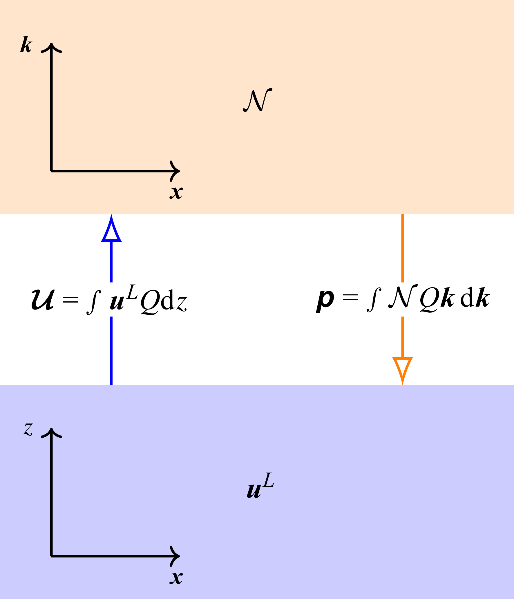
 N(x,k)
 uL(x,z)
 p(x,z)
 U(x,κ)

 α=f
 uL(z,t)/p⋆(z)
 vL(z,t)/p⋆(z)
 =|uL|2/2p⋆2
 p⋆(z)2
 α/f=1

 Open access

