Introduction
Reflecting the importance of central vision in primate behavior, the vast majority of psychophysical and physiological investigations of the visual system have tended to concentrate on the foveal and the parafoveal parts of the visual field. Thus, even today, very little is known about the neural processing of visual information in the far periphery of the visual field (eccentricity > 50°), where binocular vision is absent and acuity is low. In general, the underlying assumption has been that visual processing is invariant across the entire visual field (Hubel & Wiesel, Reference Hubel and Wiesel1974), with changes in perceptual performance being primarily dictated by the dramatic fall in the cortical magnification factor with eccentricity, and the concomitant increase in receptive field sizes in the primary visual area, V1 (M-scaling; Rovamo et al., Reference Rovamo, Virsu and Näsänen1978; Virsu & Rovamo, Reference Virsu and Rovamo1979; Pointer, Reference Pointer1986). According to this view, peripheral vision would be expected to perform as a scaled-down (low acuity) version of central vision.
There are, however, good reasons to suspect that vision in the far periphery may also be specialized in its own way, given that the rapid detection of transient events at the edge of sight is of clear importance for survival (e.g., To et al., Reference To, Regan, Wood and Mollon2011). For example, it has been demonstrated that visual information in the far periphery exerts a disproportionate influence in determining sensations of self-motion and in initiating rapid posture and body orientation reactions (Brandt et al., Reference Brandt, Dichgans and Koenig1973; Berthoz et al., Reference Berthoz, Pavard and Young1975; Bessou et al., Reference Bessou, Séverac Cauquil, Dupui, Montoya and Bessou1999). Furthermore, far peripheral vision shows subtle, but significant differences in motion processing, in comparison with central vision (Yu et al., Reference Yu, Verma, Yang, Tibballs, Lui, Reser and Rosa2010). Conversely, there are also suggestions that peripheral vision may be inferior to central vision beyond what is predicted by simple spatial scaling. For example, M-scaling is insufficient to equate the performance of central and peripheral vision in various psychophysics tasks, such as phase discrimination and face recognition (Stephenson et al., Reference Stephenson, Knapp and Braddick1991; Mäkelä et al., Reference Mäkelä, Näsänen, Rovamo and Melmoth2001; Strasburger et al., Reference Strasburger, Rentschler and Jüttner2011). It is therefore likely that some neural processes show relative degradation with increasing eccentricity and could even be completely absent in the far periphery.
Differences between central and peripheral vision could be underpinned by quantitative differences in the response properties of cortical neurons. This possibility has been highlighted by anatomical tracing studies, which have shown that the representations of the central and the peripheral visual fields in various cortical areas, including V1, receive different sets of cortico-cortical afferents (Sousa et al., Reference Sousa, Piñon, Gattass and Rosa1991; Rosa et al., Reference Rosa, Soares, Fiorani and Gattass1993; Gattass et al., Reference Gattass, Sousa, Mishkin and Ungerleider1997; Palmer & Rosa, Reference Palmer and Rosa2006), suggesting that they may perform different functions (Yu et al., Reference Yu, Chaplin, Davies, Verma and Rosa2012).
One problem with understanding the relationship between perception and neural computations across different parts of the visual field is the paucity of physiological studies that systematically addressed the response properties of neurons in the representation of the far periphery of primate V1. Although some aspects of spatiotemporal processing in the far peripheral representation in this area have been shown to be different from those of the central representation (Yu et al., Reference Yu, Verma, Yang, Tibballs, Lui, Reser and Rosa2010), other aspects, such as selectivities for orientation, direction of motion, and stimulus size, have not been characterized in any detail. The present study addresses this issue by characterizing several basic response properties at different eccentricities. We found that, superimposed on the near-uniformity of V1, there are subtler physiological variations, which may have impact on perception.
Materials and methods
Single- and multi-unit extracellular recordings were obtained from 16 adult New World monkeys (common marmoset, Callithrix jacchus), in acute sessions that also included recordings from other areas not described here. The experiments were conducted in accordance with the Australian Code of Practice for the Care and Use of Animals for Scientific Purposes. All procedures were approved by the Monash University Animal Ethics Experimentation Committee.
Preparation
The preparation for single- and multi-unit recordings followed a protocol that was slightly modified from that described by Bourne and Rosa (Reference Bourne and Rosa2003). Anesthesia was induced with alfaxalone (Alfaxan, 10 mg/kg; Jurox, Rutherford, Australia), allowing a tracheotomy, a vein cannulation and a craniotomy to be performed. After all surgical procedures were completed, the animal was administered an intravenous infusion of pancuronium bromide (0.1 mg/kg/h; Organon, Sydney, Australia) combined with sufentanil (6 µg/kg/h; Jassen-Cilag, Sydney, Australia) and dexamethasone (0.4 mg/kg/h; David Bull, Melbourne, Australia), after which it was artificially ventilated with a gaseous mixture of nitrous oxide and oxygen (7:3). The electrocardiogram and SpO2 level were continuously monitored. Administration of atropine (1%) and phenylephrine hydrochloride (10%) eye drops (Sigma Pharmaceuticals, Melbourne, Australia) resulted in mydriasis and cycloplegia. Appropriate focus and protection of the cornea from desiccation were achieved by means of appropriate contact lenses, which brought into focus the surface of a calibrated monitor (Sony Multiscan G520, 100 Hz refresh rate). The surface of the monitor’s screen was located 50–100 cm in front of the animal’s eyes, the distance varying depending on whether the central or peripheral representation was explored in a given experiment. To prevent possible differences in the optical quality of the eyes during these long (>48 h) recording sessions from confounding the results, visual stimuli were presented monocularly to the eye contralateral to the hemisphere from which the neuronal recordings were obtained (the ipsilateral eye was occluded). We were always able to elicit robust responses from the contralateral eye because the vast majority of neurons in adult marmoset’s V1 show balanced responses to the two eyes, and strong dominance by the ipsilateral eye is particularly rare (Sengpiel et al., 1996).
Electrophysiological recordings
Parylene-coated tungsten microelectrodes (∼1 MΩ), with exposed tips of 10 µm (WE3001XXF; MicroProbe, Fremont, CA), were directed toward visual area V1 using stereotaxic coordinates obtained in the course of previous studies (Fritsches & Rosa, Reference Fritsches and Rosa1996; Chaplin et al., Reference Chaplin, Yu and Rosa2013). The electrode was slowly advanced into the cortex through a small slit in the dura mater, until the first units could be observed above background activity. To avoid recording instability due to brain pulsation, the craniotomy was covered with a 2–4-mm thick layer of warm agar (2%), which was further protected with melted bone wax when necessary. Amplification and filtering (bandpass 300–5 kHz) of the electrophysiological signal was achieved by a Model 1800 Microelectrode AC amplifier (AM Systems, Everett, WA) and a 50 Hz line-noise filter (HumBug; Quest Scientific, Vancouver, Canada). Some data were collected using A/DVANCE software (designed by Robert Douglas, University of British Columbia) running on a Power Macintosh computer for stimulus generation and data acquisition. In this set-up, the signal was initially fed into a waveform discriminator (SPS-8701; Signal Processing Systems, Adelaide, Australia), allowing the isolation of single-unit signals by means of a template-matching algorithm. The remainder of the data were collected with Expo software (designed by Professor Peter Lennie), which also allows for online spike discrimination. Data collected with the two systems were consistent with each other.
The spatiotemporal tuning of cells was compared in three regions of V1, defined according to receptive field eccentricity: central vision (3–5° eccentricity), near peripheral vision (5–15° eccentricity), and far peripheral vision (>50° eccentricity). Units of the central group were sampled from the dorsal surface of caudal V1, approximately 1.5 mm from the border of V1 with the second visual area (V2), whereas near peripheral units were recorded from the caudal part of the medial wall and caudal part of the dorsal bank of the calcarine sulcus. Far peripheral units were recorded from the rostral tip of the calcarine sulcus, about 8 mm from the occipital pole and 8 mm from the midline (Fritsches & Rosa, Reference Fritsches and Rosa1996).
Quantitative tests
Within each electrode penetration, neurons were sampled at approximately 100 μm intervals. At each location, the boundary of the minimum response receptive field was first mapped using manually operated stimuli (high-contrast moving bars and gratings as well as flashing light spots) displayed on a computer monitor while the experimenter monitored the multiunit activity through a loud speaker. A high-contrast moving bar was used to draw an approximate outline of the receptive field. A small flashing light spot or bar (typically smaller than one-third of the receptive field) was then used to refine the boundary. This stimulus was placed in stationary positions inside the receptive field outline, and we ensured that every dark/bright cycle elicited responses. The same procedure was also used to estimate the functional center of the receptive field (the point that elicited the maximal response; see Lui et al., Reference Lui, Bourne and Rosa2006). Finally, small patches of drifting grating were placed outside the estimated boundary of the receptive field to check that no responses could be elicited. The waveforms of the largest units were then isolated (using either SPS-8701 or Expo’s spike discrimination function) while a drifting grating was displayed over the receptive field. Following a qualitative estimate of the cell’s selectivity using manually operated drifting gratings of varying orientations, sizes, and spatiotemporal characteristics, a series of quantitative tests was conducted. Each test condition was repeated eight times, with each grating presentation lasting 2 s. The intertrial interval was 500 ms. The midpoints of the gratings were centered on the most sensitive parts of the manually delineated minimal response fields, defined as explained above. Except for the summation tests where the size of the gratings varied, the diameters of the gratings were set to approximately twice the diameter of the minimal response fields. This was done to avoid stimulation of the receptive fields by other spatial frequencies and orientations, which exist at stimulus borders.
The quantitative study of each unit started with determination of the optimal orientation and direction of motion, using gratings that drifted in 18 directions (in 20° steps). This was followed by characterization of the spatiotemporal tuning properties at near-optimal direction. For about half of the units, this was performed independently by varying the spatial frequency and the temporal frequency of sine wave gratings, according to a matrix that included 25 or 36 combinations of values of these variables. This procedure allowed for possible interactions between spatial frequency and temporal frequency tuning, which were, however, found to be very rare in V1 (Yu et al., Reference Yu, Verma, Yang, Tibballs, Lui, Reser and Rosa2010). Thus, in studying the other half of the units, the spatial frequency tuning curve was first measured, with the temporal frequency tuning curve being subsequently measured using a grating of near-optimal direction and spatial frequency. Finally, the size summation tuning curve was measured with high-contrast (>0.8) gratings of near optimal direction, spatial frequency, and temporal frequency, which varied in diameter. The largest grating diameters used were 10° for the central (C) and near peripheral (NP) groups, and 30° for the far peripheral (FP) group. These limit values were in all cases significantly larger than the diameters of minimum response fields (MRFs) of marmoset V1 neurons at equivalent eccentricities (C group MRF: mean = 1.0°, range 0.5–2.5°; NP group: mean = 2.3°, range 0.8–5°; and FP group: mean = 8.8°, range 3–20°; Rosa et al., Reference Rosa, Fritsches and Elston1997; Chaplin et al., Reference Chaplin, Yu and Rosa2013).
Data analysis
Response linearity
The linearity of a neuron’s responses to sinusoidal gratings was quantified by the ratio between the amplitude of the first harmonic component and the mean firing rate (F1/F0; De Valois et al., 1982b; Skottun et al., Reference Skottun, De Valois, Grosof, Movshon, Albrecht and Bonds1991). During these tests, the parameters of the gratings (direction, spatial frequency, and temporal frequency) were kept at near-optimal values for the neurons, based on the series of quantitative tests outlined above. We used the mean firing rate above the spontaneous rate to characterize the tuning properties of all cells.
Direction and orientation tuning
Direction and orientation selectivity were quantified using the vector sum method (Swindale, Reference Swindale1998; Ringach et al., Reference Ringach, Shapley and Hawken2002). For this calculation, let R(θ j ) denote the above-spontaneous firing rate of a neuron’s response to a grating drifting at direction θ j (0° ≤ θ j < 360°, j = 0, 1, … n). The k-th sample moment of the tuning curve is a vector (expressed in the complex plane) defined as follows:
 $${M_k} = \sum\limits_{j = 0}^n {R\left( {{\theta _j}} \right){{\rm{e}}^{ - i \cdot k \cdot {\theta _j}}}} .$$
The normalized magnitude of the first sample moment, which will be referred to as cv360, was used to quantify direction selectivity:
 $${\rm{cv}}360 = 1 - {{\left| {{M_1}} \right|} \over {\sum\nolimits_{j = 0}^n {R\left( {{\theta _j}} \right)} }}.$$
Similarly, the normalized magnitude of the second sample moment, which will be referred to as cv180, was used to quantify orientation selectivity:
 $${\rm{cv}}180 = 1 - {{\left| {{M_2}} \right|} \over {\sum\nolimits_{j = 0}^n {R\left( {{\theta _j}} \right)} }}.$$
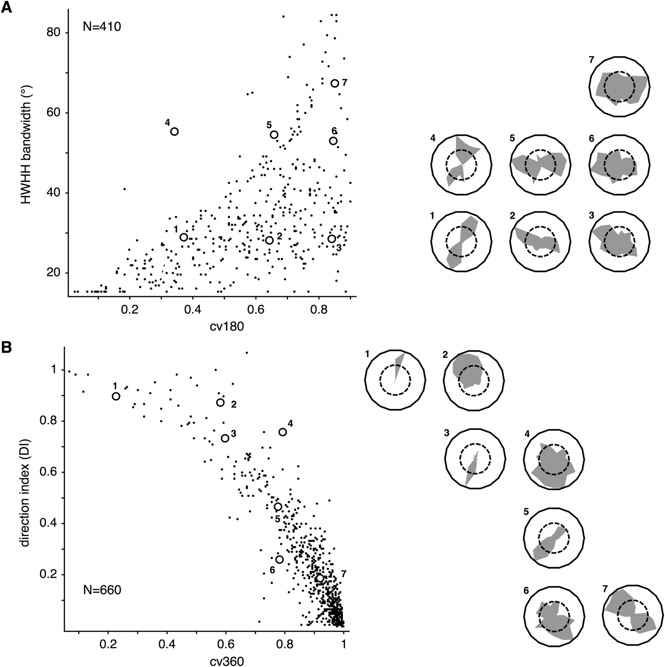
Both cv360 and cv180 range from 0 to 1, with higher values indicating lower selectivity. More traditional measures, such as the direction index (DI) for direction selectivity and half-width half-height (HWHH) bandwidth for orientation selectivity, were also calculated for comparison. These are local measures, which only summarize data points around the peak. In contrast, measures based on vector sums take all data points into account and therefore are more able to reflect the global shapes of the tuning curves (Ringach et al., Reference Ringach, Shapley and Hawken2002). The relationship between HWHH bandwidth and cv180 in our sample is illustrated in Fig. 1A. By comparing data points along the same row (1–3 or 4–6), it can be appreciated that tuning curves with similar HWHH bandwidth can be mapped to very different values of cv180. This is because the neuronal responses in orthogonal directions can vary from cell to cell, with this variation not being reflected in the HWHH bandwidth measurements. For comparison of different measures of direction selectivity, we plot in Fig. 1B the joint distribution of DI and cv360. This relationship is nonlinear but more correlated (Spearman’s rank correlation coefficient = −0.85, in comparison with 0.61 between cv180 and HWHH), with cells showing higher DI values also showing lower cv360 values.
The relationship between measures of orientation and direction selectivity based on the vector sum methods (cv180 and cv360) and local measures (HWHH bandwidth and DI). (A) Second-order circular variance (cv180) and HWHH bandwidth were used to quantify the orientation selectivity of 410 neurons. Direction-selective cells (cv360 < 0.8) and broadly tuned cells (cv180 > 0.9) were excluded from this plot. The tuning curves of a few units (indicated by numbers) are illustrated on the right in polar coordinates. Vertices on the shaded polygons in the polar plots represent the above-spontaneous response rates to each direction. The dashed lines represent half the normalized response rate. (B) First-order circular variance (cv360) and DI were used to quantify direction selectivity.

To estimate the preferred direction of a neuron, the direction tuning curve was fitted to a mixture model (f) of two von Mises functions (f v) of equal concentration, with peaks set 180° apart.
 $$\eqalign{ & f\left( {\theta ;\mu ^ * ,\kappa ,a_1 ,a_2 ,r_0 } \right) = r_0 + a_1 f_{\rm{v}} \left( {\theta ;\mu ^ * ,\kappa } \right) + a_2 f_v \left( {\theta ;\mu ^ * + \pi ,\kappa } \right) \cr & f_{\rm{v}} \left( {\theta ;\mu ^ * ,\kappa } \right) = \exp \left( {\kappa \cdot \cos \left( {\theta - \mu ^ * } \right)} \right), \cr} $$
where 0° ≤ μ* < 360° is the optimal direction, κ ≥ 0 is the concentration parameter, r 0 ≥ 0 is the baseline firing rate, and a 1 ≥ 0 and a 2 ≥ 0 are scaling parameters. We first estimated μ*, using the method described in Fisher (Reference Fisher1993, p. 99), and then fit the other three parameters with least-square nonlinear optimization. The HWHH bandwidth was also calculated from the fitted curve as a complementary measure of orientation selectivity. The uniformity of preferred orientation and direction was tested using the circular statistics package (CircStats) for R (http://www.r-project.org).
Spatial frequency tuning
Many of the cells that form the present sample were also analyzed as part of a previous study (Yu et al., Reference Yu, Verma, Yang, Tibballs, Lui, Reser and Rosa2010) in which the spatial and temporal frequencies of the grating were varied independently. In these cases, determination of the optimal, spatial, and temporal frequencies was based on the fitting of a tuning surface as described in Yu et al. (Reference Yu, Verma, Yang, Tibballs, Lui, Reser and Rosa2010). For the remainder of the data, the spatial and temporal frequency tuning curves were measured separately and fitted with Gaussian functions.
Grating diameter tuning
Diameter tuning curves were fitted with three competing models of increasing complexity. The Bayesian information criterion (BIC) was then used to select the best model. The BIC is a method of model selection that trades off goodness-of-fit with model complexity, so that more complex models do not dominate by overfitting (Yu et al., Reference Yu, Verma, Yang, Tibballs, Lui, Reser and Rosa2010). The three models that were fitted to each cell’s data were:
-
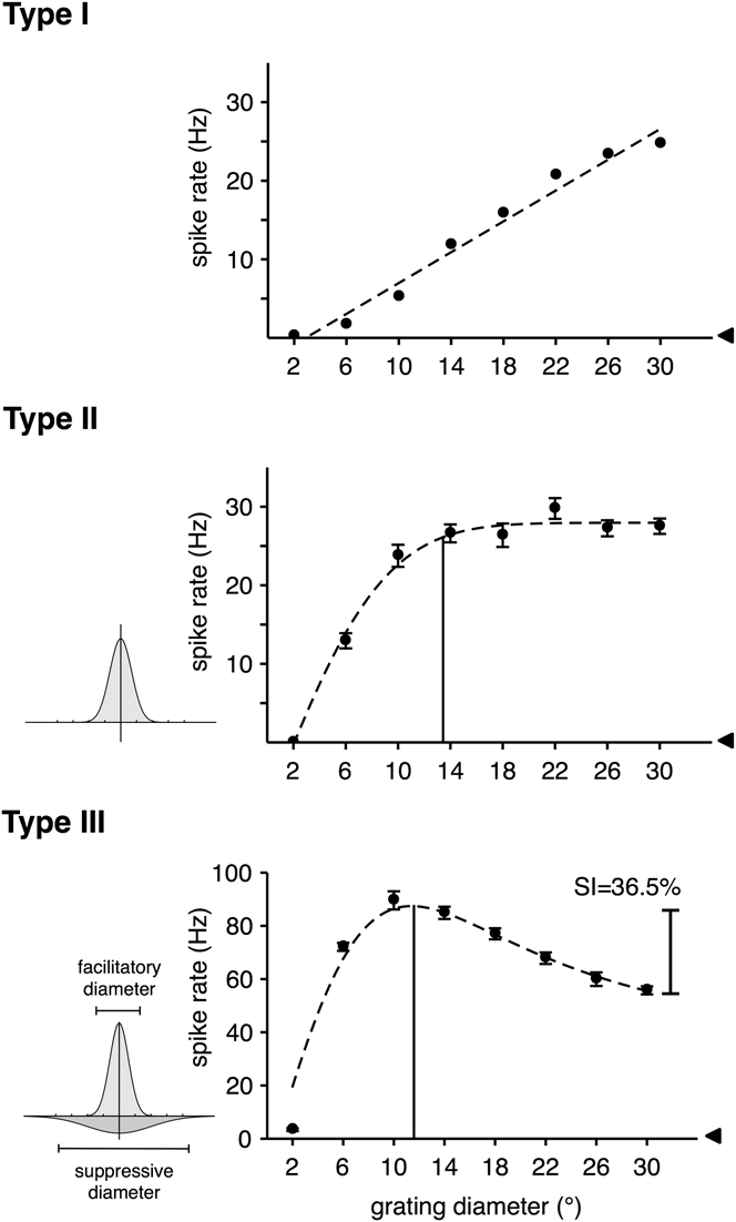
(1) R I(d): a linear model, which assumes that the response rate increases with diameter (d) without saturation (Fig. 2, top).
-
(2) R II(d): models the summation behavior of the neuron as consisting of a single facilitatory component, expressed as a Gaussian function (Fig. 2, middle). The summation curve is therefore described by
 $${R_{{\rm{II}}}}\left( {d;{r_0},{a_ + },{s_ + }} \right) = {r_0} + {a_ + } \cdot {\rm{erf}}\left( {{d \over {{s_ + }}}} \right),$$
where d is the diameter of the grating, r 0, a +, s + are scaling parameters, and erf is the error function. Unlike R I, R II saturates at a certain point.
-
(3) R III(d): models the summation behavior of the neuron as consisting of one facilitatory component and one suppressive component (DeAngelis et al., Reference DeAngelis, Robson, Ohzawa and Freeman1992; Sceniak et al., Reference Sceniak, Ringach, Hawken and Shapley1999), both expressed as Gaussian functions (Fig. 2, bottom). The summation curve is therefore described by
 $${R_{{\rm{III}}}}\left( {d;{r_0},{a_ + },{s_ + },{a_ - },{s_ - }} \right) = {r_0} + {a_ + } \cdot {\rm{erf}}\left( {{d \over {{s_ + }}}} \right) - {a_ - } \cdot {\rm{erf}}\left( {{d \over {{s_ - }}}} \right).$$
Examples of responses to near-optimal drifting gratings as functions of grating diameter. These three neurons, recorded in the far periphery, exemplify the classification of V1 cells into three groups. The error bars represent standard errors of the mean, and the arrowheads indicate spontaneous response rates. The dashed curves illustrate the best-fitted functions. The vertical lines in the main panels indicate estimates of the GSF for type II and type III cells (corresponding to the grating diameter that elicited the maximal response). Suppression index (SI) was used to quantify the amount of suppression in type III neurons.

If R I was selected by BIC as the best model for a neuron, it was classified as a type I neuron. Type II and type III neurons are those that were best fitted by either R II or R III.
For a type II or type III neuron, the grating summation field (GSF) was calculated as the grating diameter that maximized the response. For type III neurons, the diameters of the facilitatory and the suppressive Gaussian components were calculated as the size of the two components—defined as the intervals over which integrals amounted to 95% of the total areas of the Gaussians (see the bottom row of Fig. 2). Suppression Index (SI) was calculated as the difference between R III at the peak and at the largest grating diameter tested, divided by R III at the peak.
Histology
At the end of the experiments, the animals were administered an overdose of sodium pentobarbitone (Rhone-Merieux, Brisbane, Australia) and perfused transcardially with 0.9% saline, followed by 4% paraformaldehyde in 0.1 M phosphate buffer (pH 7.4). After cryoprotection by increasing concentrations of sucrose, and sectioning, alternate slides (40 µm) were stained for Nissl substance for reconstruction of electrode tracks relative to histological borders. In some animals, alternate series of sections were also stained for myelin (Gallyas, Reference Gallyas1979) and cytochrome oxidase (Wong-Riley, Reference Wong-Riley1979). The electrode tracks were reconstructed with the aid of small electrolytic lesions (4 µA, 10 s), which were placed at various sites during the experiments. The laminar distribution of the recorded units was classified into three categories: supragranular layers, layer 4, and infragranular layers. Layer 4 was defined according to Hassler (Reference Hassler, Hassler and Stephen1966) and corresponded to Brodmann’s layer 4c. The latter could always be identified physiologically during the experiments due to a combination of small receptive fields and high spontaneous activity.
Results
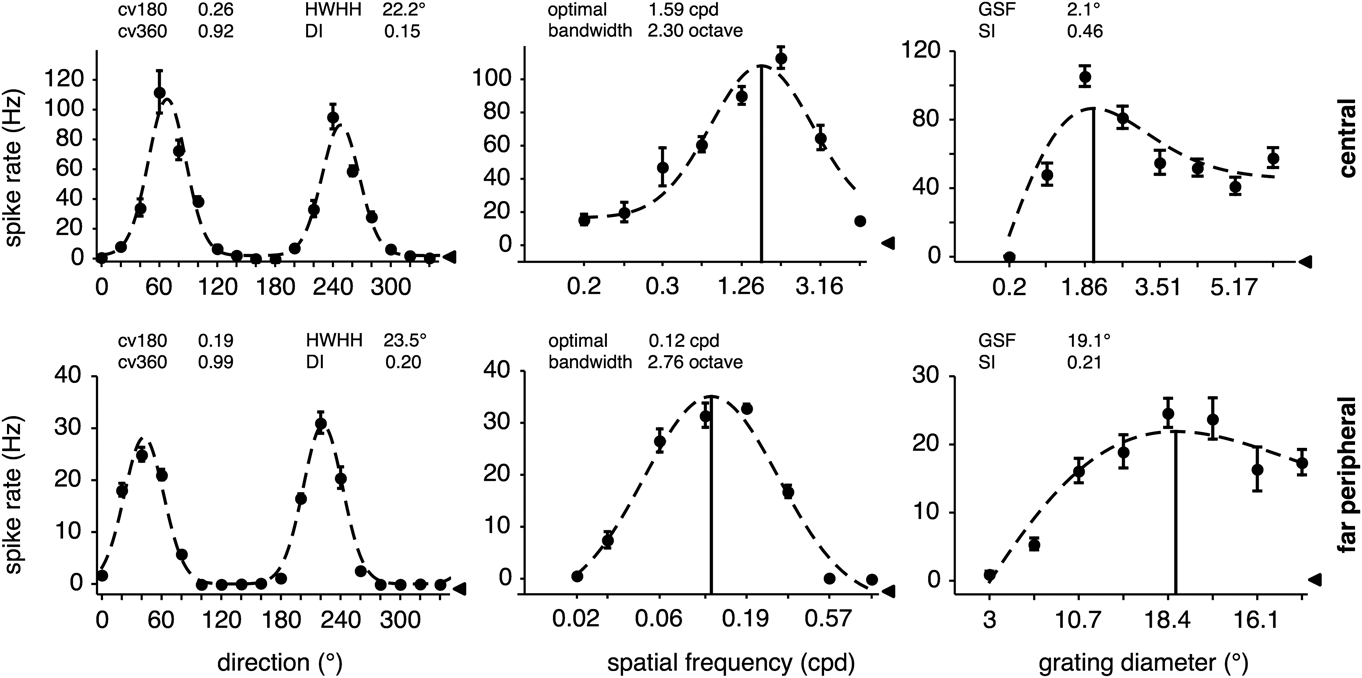
We obtained direction, spatial frequency, temporal frequency, and summation tuning curves using drifting gratings for cells with receptive fields within three ranges of eccentricity: central (C: 3–5° in eccentricity), near peripheral (NP: 5–15° in eccentricity), and far peripheral (FP: >50° in eccentricity). Representative tuning curves obtained from cells in the C and FP groups are shown in Fig. 3.
Direction, spatial frequency, and grating summation tuning curves from two neurons, one representing central vision (top row) and the other far peripheral vision (bottom row). The error bars represent standard errors of the mean. The leftward arrowheads indicate spontaneous response rates. The vertical bars mark the optimal values for grating parameters. Abbreviations: cv, circular variance; HWHH, half-width half-height orientation bandwidth; DI, direction index; cpd, cycles per degree; GSF, grating summation field; and SI, suppression index.

Response linearity
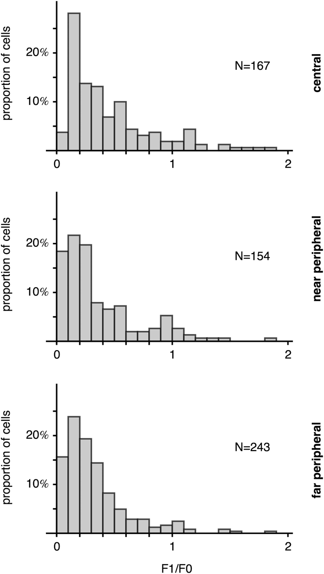
The distributions of the ratio between the amplitude of the first harmonic component and the mean firing rate (F1/F0) in our sample are plotted in Fig. 4. A total of 564 neurons (167 in the C group, 154 in the NP group, and 243 in the FP group) located in the supragranular and infragranular layers were used in this analysis. The proportions of simple cells (F1/F0 > 1) in this sample were 15.0 ± 5.4, 7.8 ± 4.5, and 4.9 ± 2.7% for the C, NP, and FP groups, respectively (the error margins indicate 95% bootstrap confidence intervals). The C group contained a significantly higher percentage of simple cells (permutation test; C vs. NP: P = 0.023; C vs. FP: P < 0.001). The difference between the two peripheral groups was not significant (NP vs FP: P = 0.1204). Only the NP group showed a significant difference in the proportion of simple cells in the supragranular and the infragranular layers (supragranular: 1.7 ± 2.6%; infragranular: 11.5 ± 6.8%; permutation test: P = 0.016). It should be noted that the gratings used in our measurements were larger than the size of the receptive fields, which could have affected response linearity (Bardy et al., Reference Bardy, Huang, Wang, FitzGibbon and Dreher2006). The degree to which nonclassical receptive field influences response linearity in the near and far peripheral visual fields is unknown and requires further study.
The distribution of F1/F0 in cells belonging to the three eccentricity groups. F1/F0, a measure of response linearity, is the ratio between the amplitude of the first harmonic component of the response (F1) and the mean firing rate (F0). Samples collected from cortical layer 4 were excluded from this figure.

Selectivity to the direction of motion and orientation
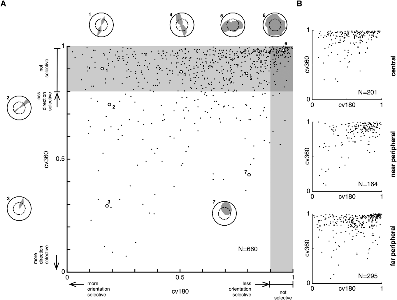
Orientation and direction tuning curves were obtained from 201 units in the C group, 164 units in the NP group, and 295 units in the FP group. Direction selectivity was quantified primarily by the first-order circular variance (cv360), and orientation selectivity was quantified primarily by the second-order circular variance (cv180). The variety of direction tuning curves we observed in V1 can be visualized in the 2D plane by plotting the joint distributions of cv180 and cv360 (Fig. 5A). The distributions for the three eccentricity groups (C, NP, and FP) were similar (Fig. 5B), with no difference in the distributions being detected by Bivariate Kolmogorov–Smirnov tests (C vs. NP: D = 5.34544, P = 0.614; NP vs. FP: D = 4.97352, P = 0.601; C vs. FP: D = 6.01213, P = 0.639).
(A) The joint distribution of cv180 and cv360 for all neurons in the data set. A number of examples of tuning curves (numbered from 1 to 7) are illustrated. (B) The distributions of these parameters according to the three eccentricity groups.

Direction selectivity
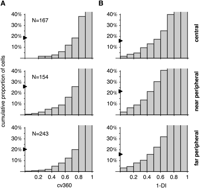
The cumulative distribution of cv360 for cells located outside layer 4 is plotted in Fig. 6A. Using cv360 < 0.8 as the criterion for direction selectivity, we estimated that 21.3 ± 3.5% of neurons in this sample were direction selective (ds) (95% bootstrap confidence interval). Simple cells were more likely to be ds than complex cells (30.6 ± 13.3% vs. 20.4 ± 3.3%; P = 0.04 by permutation test). The proportions of ds neurons for the C, NP, and FP groups were 18.6 ± 6.0, 26.0 ± 7.1, and 20.2 ± 5.1%, respectively. The differences were not significant (permutation test; C vs. NP: P = 0.054; NP vs. FP: P = 0.087; C vs. FP: P = 0.3441). A more traditional criterion, based on the DI (DI > 0.5, Fig. 6B), revealed a very similar pattern: the proportion of ds neurons was 16.8 ± 3.1% for the entire population and 13.2 ± 5.1, 21.4 ± 6.5, and 16.5 ± 4.7% for the C, NP, and FP groups, respectively. According to this criterion, the NP group showed a slightly higher proportion of ds cells than the C group (permutation test; C vs. NP: P = 0.024), but other comparisons (C vs. FP and NP vs. FP) revealed no significant difference. In summary, the proportions of ds neurons did not change dramatically across the entire range of eccentricities in V1.
Comparing direction selectivity across the three eccentricity groups. (A) The cumulative distribution of cv360. The percentages of neurons with cv360 < 0.8 are indicated by the arrows. The y-axis is truncated to allow better visualization of the distributions of cells with low cv360 (i.e., strong direction selectivity). (B) The cumulative distribution of 1-DI, where DI is the direction index. The arrows indicate the percentages of neurons with DI > 0.5. Samples collected from layer 4 were excluded from this figure.

Direction selectivity was dependent on cortical layers. When the three eccentricity groups were pooled, the cv360 < 0.8 criterion indicated that ds neurons were more common in infragranular layers (32.2 ± 5.9%) than in supragranular layers (13.8 ± 3.7%). The difference was significant (permutation test; P < 0.001). The same conclusion was reached when the eccentricity groups were analyzed separately. In layer 4, we did not encounter ds cells.
Orientation selectivity
As a measure of the sharpness of orientation tuning, cv180 is appropriate only for tuning curves with two peaks that are 180° apart. We therefore restricted our analysis of cv180 to nondirective-selective (nds) cells (using the cv360 > 0.8 criterion). For neurons sampled in the supragranular and the infragranular layers across the entire data set, the median value of cv180 was 0.64. Simple cells were slightly more broadly tuned for orientation than complex cells (median cv180 was 0.73 for simple cells and 0.63 for complex cells. Mann–Whitney U = 8473, P = 0.037). As in other species of monkey (Rosa et al., Reference Rosa, Gattass, Fiorani and Soares1992; Ringach et al., Reference Ringach, Shapley and Hawken2002), layer 4 cells tended to be less orientation selective (median cv180: 0.90, 0.91, and 0.93 for C, NP, and FP, respectively).
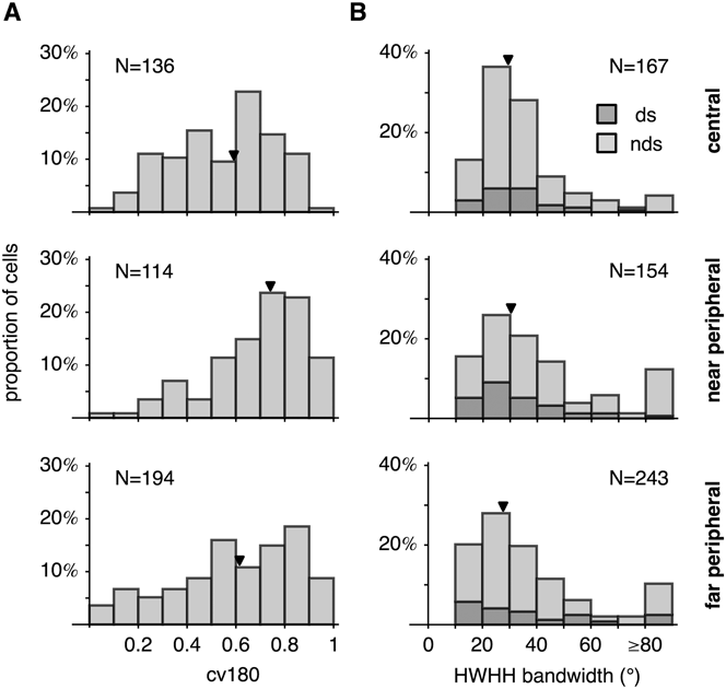
The distributions of cv180 are illustrated in Fig. 7A. The median values were 0.59, 0.74, and 0.62 for the C, NP, and FP groups, respectively. There were significant differences among eccentricity groups (Kruskal–Wallis K = 26.3964, P < 0.001) but there was no consistent increase or decrease in orientation selectivity as a function of eccentricity. All pairwise comparisons showed significant differences (C vs. NP: Mann–Whitney U = 4706, P < 0.001; NP vs. FP: U = 13,381, P = 0.002; C vs. FP: U = 11,278, P = 0.025).
Comparing orientation selectivity across the three eccentricity groups. Samples collected from layer 4 were excluded from this figure. (A) The distributions of cv180. The arrowheads indicate median values. Ds neurons (cv360 < 0.8) were excluded from the analysis. (B) Distributions of HWHH bandwidth. The regions shaded in dark and light gray indicate the proportions of cells that were ds and nds, respectively. The arrowheads represent median values. Broadly tuned cells (HWHH greater than or equal to 80°) were excluded from the calculation of the medians.

In addition to comparing median values, it is also useful to compare the proportion of cells that are too broadly tuned to be considered orientation biased. Using cv180 > 0.9 as a criterion, the percentage of broadly tuned neurons was 0.7 ± 1.1% (C group), 11.4 ± 5.7% (NP group), and 8.8 ± 3.9% (FP group) for the three groups in our samples (95% bootstrap confidence interval). The C group had significantly fewer broadly tuned cells than the other two groups (permutation test; C vs. NP: P < 0.001; NP vs. FP: P = 0.2366; C vs. FP: P < 0.001).
Orientation selectivity can also be quantified by the HWHH bandwidth (Fig. 7B). As HWHH bandwidth is a local measure, it can be used to characterize ds cells as well as nds cells. The analysis therefore did not exclude ds cells (as we did in the analysis based on cv180). However, we excluded neurons for which the tuning curves were so broad that HWHH bandwidth could not be estimated, and those for which HWHH was larger or equal than 80°. The proportions of broadly tuned cells that were excluded were 4.2 ± 3.3% (C group), 12.3 ± 5.2% (NP group), and 10.3 ± 3.9% (FP group). Like the comparison performed with cv180, the C group had significantly fewer broadly tuned cells (permutation test; C vs. NP: P = 0.004; NP vs. FP: P = 0.2596; C vs. FP: P = 0.013). Whereas the above results suggest a mild functional gradient in V1 in terms of percentages of neurons without orientation bias, once these were removed from analysis the median values of HWHH bandwidth among the remaining cells were very similar: 29.0° (C group), 30.5° (NP group), and 28.5° (FP group). These values were not significantly different (Kruskal–Wallis K = 1.19417, P = 0.551316). The median HWHH bandwidth for the entire population was 29.0°.
In the C and the NP groups, we detected no significant difference in orientation selectivity between the supragranular cells and the infragranular cells. Median cv180 was 0.56 (supragranular) and 0.61 (infragranular) in the C group (Mann–Whitney U = 1791, P = 0.5363). In the NP group, the median was 0.74 for both the supragranular and infragranular layers (U = 1668, P = 0.7). The FP group was the only one that showed a difference. Median cv180 was 0.56 for the supragranular layers and 0.84 for the infragranular layers (U = 1491, P < 0.001).
Anisotropy in the distributions of preferred orientation and direction
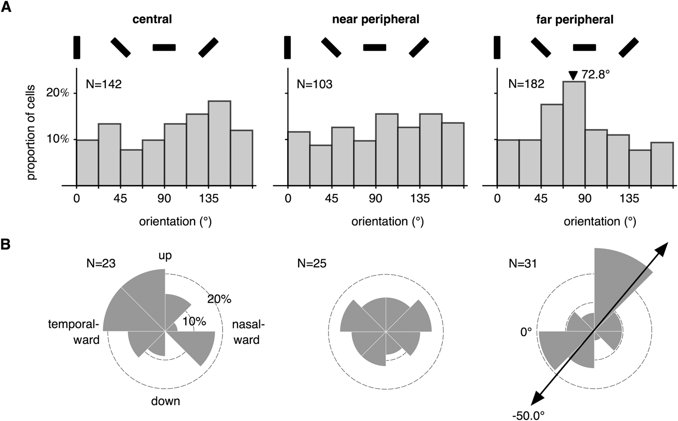
The preferred orientations for neurons that were neither ds (cv360 < 0.8) nor broadly tuned (cv180 > 0.9) are plotted in Fig. 8A. The distribution of the C group did not deviate significantly from uniformity (Rao’s spacing test; U = 136.4161, P > 0.10). The Rayleigh test, which is more powerful for detecting unimodal distributions, also did not detect any concentration toward a particular orientation (R = 0.1011, P = 0.2337). The same conclusion applied to the NP group (Rao’s spacing test: U = 144.2893, 0.05 < P < 0.10; Rayleigh test: R = 0.1219, P = 0.2168). In contrast, the FP group showed a distinct bias for orientations near the horizontal (indicated by an arrowhead in Fig. 8A; R = 0.2191, P = 0.0002). When data from the three groups were pooled, no deviation from uniformity was detected (Rao’s spacing test: U = 131.8692, P > 0.10; Rayleigh test: R = 0.075, P = 0.093). We further divided orientations into four equally spaced 45° intervals centered around the vertical, the horizontal, and the two oblique orientations. Only the histogram for the FP group showed deviation from uniformity (χ2 = 12.5055, df = 3, P = 0.0058). Finally, we also examined whether neurons preferring the cardinal orientations were more sharply tuned (Li et al., Reference Li, Peterson and Freeman2003) but found no evidence of this effect; the median cv180 values for these four intervals were not statistically different. Restricting the analyses to simple cells (F1/F0 > 1.0) also did not reveal any additional bias.
(A) The distributions of the preferred orientations for neurons that were not ds (cv360 < 0.8) and not broadly tuned (cv180 > 0.9). The black bars indicate the coding of grating orientations. The arrowhead indicates the mean orientation where a unimodal distribution was detected by the Rayleigh test. (B) The distribution of the preferred directions of motion, among ds neurons (cv360 < 0.7). The bar with arrowheads indicates an axis for which a significant bimodal clustering was detected by the Rayleigh test.

The preferred directions of the ds neurons (cv360 < 0.7) are plotted in Fig. 8B. Due to the low density of ds neurons, the populations were small (23, 25, and 31 for the C, NP, and FP groups, respectively). The only significant deviation from uniformity was in the far periphery (Rayleigh test after doubling the angles: R = 0.3512, P = 0.020), where there was a bias favoring motion along an oblique axis (50.0° rotated relative to the horizontal directions; see arrowheads in Fig. 8B). As most of our receptive fields were recorded in the lower visual field, this might indicate preference for motion toward and away from the fovea. Relaxing the criterion for direction selectivity to cv360 < 0.8 did not change these conclusions.
Grating summation
We measured summation tuning curves using high contrast (>80%) drifting gratings that were optimized for each unit in terms of orientation, spatial frequency, and temporal frequency. Three examples, all collected from the representation of the far peripheral visual field, are illustrated in Fig. 2. These three curves exemplify the types of summation behavior that we observed: type I neurons increased their firing rates in response to larger gratings, up to the maximum within the tested range (i.e., up to a diameter of 10° for the C and NP groups and 30° for the FP group). Type II neurons increased their firing rates up to a certain size (the size of the GSF or grating summation field) and then become saturated, whereas type III neurons increased their firing rates up to the size of the GSF and then showed reduced responses for larger gratings.
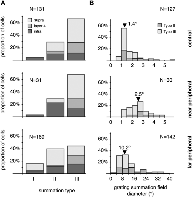
We classified 331 units (collected from five animals) into these three categories by fitting each curve using the three models, and then used the BIC to select the optimal model. The numbers of neurons used in this analysis in the C, NP, and FP groups were 131, 31, and 169. Due to the small sample size of the NP group, the present analysis concentrates on comparing central vision to far peripheral vision.
The percentages of neurons that demonstrated the different types of summation behavior are plotted in Fig. 9A. In the C group, the distribution was biased toward type III units, which represented 66.4% of the total population. The distribution for the FP group was more even, with type III cells forming 44.4% of the sample. Conversely, the population of type I neurons was small in central visual field (3.2%) but was larger in the far periphery (16.0%). The distributions of the three summation types for the C and the FP groups were significantly different (χ2 = 16.5205, df = 2, P = 0.0002). Furthermore, the laminar distributions were also affected by eccentricity (Fig. 9A). For example, type III behavior was primarily found in supragranular layers (71.4%) in the C group—an observation consistent with previous reports (Henry et al., Reference Henry, Joshi, Xing, Shapley and Hawken2013). In the FP group, however, type III behavior was more evenly distributed across the cortical layers, with supragranular layers accounting for only 33.3% of the type III cells. The laminar distributions of type III cells were significantly different between the C and the NP groups (χ2 = 10.5405, df = 2, P = 0.005142).
(A) Distributions of neurons showing different grating summation behaviors in the central (C), near peripheral (NP), and far peripheral (FP) representations of V1. (B) The distributions of the sizes of the GSFs for neurons in the three eccentricity ranges. The arrowheads indicate the median values.

The GSF of a type II or III neuron is the diameter of the region of the visual field within which progressively larger gratings elicit progressively greater response rates. The distributions of GSF values are plotted in Fig. 9B. Median GSF diameters were 1.4, 2.5, and 10.2° for the C, NP, and FP groups, respectively, which were only slightly larger than, but proportional to earlier estimates based on MRFs (1.0, 2.3, and 8.8°; Rosa et al., Reference Rosa, Fritsches and Elston1997). For the NP and FP groups, the GSF sizes for type II neurons were significantly larger than those of type III neurons (Table 1).
Diameter of the grating summation fields in different parts of V1. The diameters were measured in the visual space (°). When multiplied by the linear cortical magnification factor (Chaplin et al., Reference Chaplin, Yu and Rosa2013), we estimated the diameter of the grating summation field on the cortical surface of V1, measured in millimeters

Although the proportion of type III neurons is smaller in the far peripheral visual field than in the central visual field, our data indicate that the strength of suppression is, on average, stronger in the far periphery (Fig. 10A). The median suppression index (SI) was 56% in the far periphery, which was significantly higher than that of central vision (32%; Mann–Whitney U = 1313, P < 0.0001). In the C group, median suppression strength was the lowest for neurons sampled in cortical layer 4 (24.6%) compared with the supragranular (37.7%) and the infragranular layers (37.3%). The differences were significant (layer 4 vs. supragranular: Mann–Whitney U = 271, P = 0.0006; layer 4 vs. infragranular: U = 84, P = 0.0117; supragranular vs. infragranular: U = 385, P = 0.8824). A laminar difference in suppression strength was not observed in the FP group: suppression strength was 49.3, 56.7, and 57.7% for supragranular, layer 4, and infragranular samples, respectively. These differences were not significant (Kruskal–Wallis K = 0.39548, P = 0.8245).
(A) The distributions of the index among type III neurons. (B) The distributions of the ratio between the suppressive field diameter and the facilitatory field diameter. The arrowheads indicate median values.

As shown in Fig. 10B, the size of the suppressive field was on average about twice the size of the facilitatory field. Cells in the C and the FP groups were not significantly different in this respect (Mann–Whitney U = 3112, P = 0.612011).
Discussion
The present results expand on our earlier studies of eccentricity-dependent changes in receptive field properties in V1 (Yu et al., Reference Yu, Verma, Yang, Tibballs, Lui, Reser and Rosa2010; Chaplin et al., Reference Chaplin, Yu and Rosa2013). On the one hand, our results tell a story of uniformity: the response properties of V1 cells remain quite similar between eccentricities ranging from parafoveal (3–5°) to the temporal edge of the visual field (>50°), despite the gradual growth in receptive field size and concomitant reduction in preferred spatial frequency. On the other hand, we did detect some functional differences: the proportions of simple cells, cells without obvious orientation bias, and cells showing strong inhibitory surrounds (type III neurons) all decreased significantly from the central to the far peripheral visual field. These observations, along with our previous studies showing higher proportion of speed-tuned neurons in the far peripheral representation (Yu et al., Reference Yu, Verma, Yang, Tibballs, Lui, Reser and Rosa2010) and lower point image size in the peripheral representation in V1 (Chaplin et al., Reference Chaplin, Yu and Rosa2013), demonstrate that there are slight variations in physiological properties in different parts of V1.
Direction selectivity
Our results indicated a near-constant distribution of ds cells in V1, irrespective of receptive field eccentricity. The conclusion is in agreement with Battaglini et al. (Reference Battaglini, Galletti and Fattori1993), who characterized direction selectivity in awake, behaving macaques up to 52° of eccentricity. It is also consistent with psychophysics studies demonstrating that peripheral vision is no more sensitive to motion than central vision (van de Grind et al., Reference van de Grind, van Doorn and Koenderink1983; McKee & Nakayama, Reference McKee and Nakayama1984).
The population of ds neurons in our central vision group (C) is relatively small (18.6% using the cv360 < 0.8 criterion, and 13.2% using the DI > 0.5 criterion). These numbers are lower than estimates provided by some of the earlier studies in macaques (DI > 0.5: 29%, De Valois et al., 1982a; 27%, Orban et al., Reference Orban, Kennedy and Bullier1986; 23%, Gur et al., Reference Gur, Kagan and Snodderly2005) and marmosets (∼23.8% using the cv360 < 0.8 criterion; Forte et al., Reference Forte, Hashemi-Nezhad, Dobbie, Dreher and Martin2005) but resemble the findings of Sengpiel et al. (1996) in the parafoveal representation of marmosets (16.7%). The variations might have been related to the experimental protocols and data analysis techniques.
Orientation selectivity
We quantified orientation selectivity using the cv180 (circular variance) measure. In the central representation of V1, the median value was 0.59, which is similar to previously reported values in primate V1 (macaque: 0.61, Ringach et al., Reference Ringach, Shapley and Hawken2002; marmoset: 0.69, Forte et al., Reference Forte, Hashemi-Nezhad, Dobbie, Dreher and Martin2005). Orientation selectivity is also often quantified using the HWHH bandwidth, a local measure compared with cv180. Our median HWHH bandwidth, 29.0°, is slightly larger than that previously reported for primates (macaque: 21.0°, De Valois et al., 1982a; marmoset: 22.1°, Sengpiel et al., 1996a,Reference Sengpiel, Troilo, Kind, Graham and Blakemore b ; 25.9°, Nowak & Barone, Reference Nowak and Barone2009). This difference might be related to the finer steps used in those studies (5–15°, compared with 20° in the current study). Ringach et al. (Reference Ringach, Shapley and Hawken2002) used 15–20° steps, which were closer to our protocol, and reported that the median half-width 70%-height bandwidth was 23.5°. We adopted the same criterion and estimated the 70%-height bandwidth to be 22.0° for the central group.
With the caveat that orientation selectivity might have been slightly underestimated by the 20° sampling resolution, we concluded that many neurons in the far periphery were sharply tuned for orientation, resulting in the distributions of cv180 and HWHH bandwidth being not significantly different from those of central vision. This result is consistent with the findings of Battaglini et al. (Reference Battaglini, Galletti and Fattori1993), who reported no significant difference in orientation tuning between central (<10° eccentricity) and peripheral vision. It is also consistent with the results of psychophysics experiments showing that after appropriate scaling of stimulus size, orientation sensitivity and discrimination threshold are relatively constant across the visual field, at least until 50° eccentricity (Virsu & Rovamo, Reference Virsu and Rovamo1979; Scobey, Reference Scobey1982; Vandenbussche et al., Reference Vandenbussche, Vogels and Orban1986; Paradiso & Carney, Reference Paradiso and Carney1988). Some previous studies reported that orientation tuning becomes broader (cat: Orban & Kennedy, Reference Orban and Kennedy1981; human: Spinelli et al., Reference Spinelli, Bazzeo and Vicario1984) or sharper (monkey; De Valois et al., 1982a) with eccentricity, within more limited extents of visual field tested. Our results indicate that this effect, if exists, does not systematically extend to the far periphery, as far peripheral neurons would have to be on average very broadly or sharply tuned.
The only notable effect of eccentricity on orientation selectivity that we could identify was that the central vision group had a smaller proportion of broadly tuned cells in comparison with the other two eccentricity groups. Data in the literature are conflicting. Battaglini et al. (Reference Battaglini, Galletti and Fattori1993) compared neurons with receptive fields with eccentricity less than 10° and those in the 10–52° range and found no difference (∼25%). Livingstone and Hubel (Reference Livingstone and Hubel1984), however, found more broadly tuned cells in the foveal (36%) than in the parafoveal visual field (20%), using a qualitative assessment. Given that the presence of broadly tuned cells is dependent on the cortical layer as well as the locations in the orientation columns of the sampled cells, this inconsistency might due to sampling biases.
Orientation and direction anisotropies
Human subjects are more sensitive to horizontal and vertical orientations than to oblique orientations (Appelle, Reference Appelle1972; Orban et al., Reference Orban, Vandenbussche and Vogels1984), but only within 20° of eccentricity (Berkley et al., Reference Berkley, Kitterle and Watkins1975; Vandenbussche et al., Reference Vandenbussche, Vogels and Orban1986). Whether orientation anisotropy exists at higher eccentricities is unknown. Our data show an overrepresentation of near-horizontal orientations in the FP group, which might indicate greater sensitivity for the horizontal stimuli in the far peripheral visual field.
Physiological correlates of the oblique effect in V1 have been suggested (cat: Payne & Berman, Reference Payne and Berman1983; Li et al., Reference Li, Peterson and Freeman2003; monkey: Mansfield & Ronner, Reference Mansfield and Ronner1978; De Valois et al., 1982a; human: Furmanski & Engel, Reference Furmanski and Engel2000). The most convincing demonstration has been that of Li et al. (Reference Li, Peterson and Freeman2003), who analyzed the preferred orientation of over 4000 cells in cat V1 and found that there was an overabundance of cells preferring cardinal orientations. In our central vision group, we did not observe significant bias for preferred orientation (Fig. 8B) or changes in orientation tuning according to orientation preference. There are a few possible explanations for this discrepancy. First, our sample size might be too small. As pointed out in Li et al. (Reference Li, Peterson and Freeman2003), the oblique effect may be too subtle to be reliably detected unless thousands of samples are considered. Second, the effect may be highly dependent on eccentricity. De Valois et al. (1982a) reported anisotropy in the foveal visual space but not in the peripheral space covering the 3–5° eccentricity range, which encompasses the receptive fields of most neurons in our sample. Third, the oblique effect may be specific to certain types of receptive fields. It has been suggested that the V1 correlate of the oblique effect is primarily found in simple cells (Orban & Kennedy, Reference Orban and Kennedy1981; Li et al., Reference Li, Peterson and Freeman2003) but simple cells are underrepresented in our sample (Fig. 4).
Some preferred direction anisotropies have been reported in the peripheral visual field of the middle temporal area (Albright, Reference Albright1989; Rosa & Elston, Reference Rosa and Elston1998), although very little is known about V1. We did not find strong evidence of direction anisotropy in V1. The only exception was in the far periphery, where there was a significantly larger number of cells that preferred motion along an oblique axis that approximately linked their receptive fields to the fovea. However, it should be noted that the population of ds cells is small throughout V1, making it difficult to draw strong conclusions in this respect.
Center/surround interactions
Contextual effects in perception are believed to be physiologically mediated by center/surround mechanisms in the visual cortex, which allow stimuli outside the classical receptive field to modulate the responses of those inside the classical receptive field (Seriès et al., Reference Seriès, Lorenceau and Frégnac2003). Very little is known about the dependency of surround modulation on eccentricity, although psychophysical studies have suggested that contextual effects in the peripheral visual field can be fundamentally different from those of central vision. Hess and Dakin (Reference Hess and Dakin1997), for example, suggested that contour linking is completely missing outside 10° eccentricity. Surround suppression, however, has been reported not to operate at the fovea (Petrov et al., Reference Petrov, Carandini and McKee2005), a region of the visual field not covered by our samples. However, virtually nothing has been established about the physiological characteristics of center/surround interactions in the far periphery. The only relevant study is Battaglini et al. (Reference Battaglini, Galletti and Fattori1993), which reported no difference in the number of end-stopped V1 neurons in the central (<10°) and peripheral (10–52°) visual fields.
We studied a simple form of surround modulation: grating summation. The modulatory effect of high-contrast gratings outside the classical receptive field is primarily suppressive (Sengpiel et al., 1997; Sceniak et al., Reference Sceniak, Ringach, Hawken and Shapley1999; Jones et al., Reference Jones, Grieve, Wang and Sillito2001; Cavanaugh et al., 2002a,Reference Cavanaugh, Bair and Movshon b ). However, as reported in the literature (cat: Li & Li, Reference Li and Li1994; Walker et al., Reference Walker, Ohzawa and Freeman2000; macaque: Cavanaugh et al., 2002a), a small population of neurons with facilitatory surround (type I cells) can be found in central vision. Interestingly, the size of the population increased from 3.2% in central vision to 16.0% in the far periphery. This finding might suggest greater emphasis on spatial integration in the far peripheral visual field.
The relationship between the strength of suppression and eccentricity is unclear. Human psychophysics studies have demonstrated that the strength of surround suppression increases with eccentricity up to 10° eccentricity (Xing & Heeger, Reference Xing and Heeger2000). However, the functional MRI data reported in Williams et al. (Reference Williams, Singh and Smith2003) claimed that suppression gives way to facilitation in peripheral vision. Our comparison of central versus far peripheral data suggests a more complicated picture: although the proportion of type III neurons was reduced in the far periphery, the strength of suppression among these cells was stronger. Therefore, the nature of center/surround interactions is likely to depend on the balance of a number of factors.
The inverse relationship between receptive field size and cortical magnification suggests the possibility that equal amounts of the visual cortex are used to represent receptive fields throughout V1 (Hubel & Wiesel, Reference Hubel and Wiesel1974). We examined this hypothesis by converting the diameters of the GSF (expressed in degrees) to the diameter of the V1 representations of the GSFs (expressed in mm), using the linear cortical magnification function of marmoset V1 reported by Chaplin et al. (Reference Chaplin, Yu and Rosa2013). At the median eccentricities of the three groups (C: 3.5°, NP: 10°, and FP: 55°), the cortical magnifications are 1.060, 0.398, and 0.066 mm/°, respectively (square root of eqs. 9 in Chaplin et al., Reference Chaplin, Yu and Rosa2013). The median diameters of the GSFs therefore correspond to 1.48, 1.00, and 0.67 mm, respectively (see also Table 1). The decreasing numbers indicate deviation from the uniform model of V1 but are in agreement with the observation that the cortical representation of the MRFs also decreases in size with eccentricity (Gattass et al., Reference Gattass, Sousa and Rosa1987; Rosa et al., Reference Rosa, Gattass and Soares1991; Chaplin et al., Reference Chaplin, Yu and Rosa2013). Notably, for type III neurons, the ratio between the diameter of the facilitatory center and the diameter of the suppressive surround did not vary between the C and the FP groups. The spatial arrangement of center/surround receptive fields of individual cells in the far periphery is therefore quite similar to that of cells in the central visual field.
Conclusions
For the fovea-dominated primate visual system, spatial vision is highly dependent on eccentricity. Based on quantification of single-unit responses to well-characterized V1 response properties, we conclude that V1 can be regarded, as a first approximation, as near uniform. As proposed by Hubel and Wiesel (Reference Hubel and Wiesel1974), the most obvious differences between central and peripheral representations derive from the gradual decrease in cortical magnification factor and the concomitant increase in receptive field size (which together lead to equally obvious changes in optimal spatial frequency and thus resolution). No changes of similar magnitude exist for any of the properties measured here or for temporal frequency selectivity (Yu et al., Reference Yu, Verma, Yang, Tibballs, Lui, Reser and Rosa2010, present results). However, our results support the notion that small deviations from uniformity do exist. These observations suggest that the neuronal processing circuits of V1 show quantitative variations from the foveal to the peripheral representation, as also hinted at by Yu et al. (Reference Yu, Verma, Yang, Tibballs, Lui, Reser and Rosa2010) and Chaplin et al. (Reference Chaplin, Yu and Rosa2013). Whether these differences derive from changes in the inputs (e.g., different proportions of retinal ganglion cells with different properties), changes in the intrinsic circuits of V1 or different emphases in connections from other cortical areas (Angelucci et al., Reference Angelucci, Levitt, Walton, Hupé, Bullier and Lund2002) will need to be determined in light of future studies combining anatomical and physiological data.
Acknowledgments
This study was funded by research grants from the National Health and Medical Research Council (grant number 1003906) and Australian Research Council Special Research Initiative on Bionic Vision and Technology (SR1000006). We thank Janssen-Cilag Pty Limited for the donation of sufentanil citrate, Katrina Worthy for the expert histological processing, and Rowan Tweedale for comments on the manuscript.