1 Introduction
In the human body there are many examples of flexible-walled vessels conveying a flow. Under certain conditions, fluid–structure interaction can promote instability which manifests as a clinical detectable (often audible) signal, such as Korotkoff noises during blood pressure measurement, wheezing in lung airways or sound production by the vocal folds; experimental and theoretical models of these flow-induced instabilities have been thoroughly reviewed elsewhere (see, for example Grotberg & Jensen Reference Grotberg and Jensen2004; Heil & Hazel Reference Heil and Hazel2011). Once properly understood, these physiological phenomena can be used to develop new clinical measurement devices, using the transition to instability as a detectable threshold for the system. For example, in a recent study we characterised the onset of retinal venous pulsations (RVP) in the human central retinal vein, where the flow of blood through the vein triggers spontaneous transition to a vigorous high-frequency pulsation once the intraocular pressure (IOP, the pressure in the eye external to the vein wall) exceeds a threshold dependent on the intracranial pressure (Stewart, Jensen & Foss Reference Stewart, Jensen and Foss2014). The predicted onset curve provides a theoretical foundation for a non-invasive method to measure the intracranial pressure for a known IOP.
In this paper we consider a theoretical model for flow through a planar (asymmetric) flexible-walled channel, devised as a two-dimensional analogue of flow through a compliant conduit in the body, first presented by Pedley (Reference Pedley1992). In particular, the set-up considered below includes rigid segments of fixed (uniform) width upstream and downstream of the flexible portion, as a model for Starling resistor experiments (e.g. Bertram Reference Bertram, Carpenter and Pedley2003; Bertram & Tscherry Reference Bertram and Tscherry2006). Models for this system vary in complexity, ranging from spatially one-dimensional models (Stewart, Waters & Jensen Reference Stewart, Waters and Jensen2009; Xu, Billingham & Jensen Reference Xu, Billingham and Jensen2013), rational asymptotic models in the limit of large Reynolds number (Jensen & Heil Reference Jensen and Heil2003; Pihler-Puzović & Pedley Reference Pihler-Puzović and Pedley2013), eigenfunction expansions based on the local stability (Stewart et al. Reference Stewart, Heil, Waters and Jensen2010) and full two-dimensional numerical simulations (Luo & Pedley Reference Luo and Pedley1996; Jensen & Heil Reference Jensen and Heil2003; Luo et al. Reference Luo, Cai, Li and Pedley2008; Liu et al. Reference Liu, Luo, Cai and Pedley2009; Liu, Luo & Cai Reference Liu, Luo and Cai2012; Xu, Billingham & Jensen Reference Xu, Billingham and Jensen2014). These models exhibit a variety of oscillatory behaviour depending on how the flow is driven, which could be with either a fixed upstream pressure or a fixed upstream flux. In addition, the behaviour of the system is heavily influenced by the choice of elastic wall properties. Previous models have employed a variety of approaches, including modelling the deformation of the wall using an ad hoc tube law (e.g. Cancelli & Pedley Reference Cancelli and Pedley1985), as a pre-stressed (i.e. tensioned) membrane (e.g. Luo & Pedley Reference Luo and Pedley1996), an elastic beam with finite bending stiffness (e.g. Luo et al. Reference Luo, Cai, Li and Pedley2008) and a thin elastic shell (e.g. Jensen & Heil Reference Jensen and Heil2003). In this study we model the flexible wall as a tensioned membrane with a large pre-stress, which is assumed to dominate the other elastic restoring forces. The effects of wall mass and damping are also ignored for simplicity.
For flow driven by a prescribed upstream pressure the primary global instability for large membrane tension (so that the wall is almost flat) has been shown to be a so-called ‘sloshing’ mode driven by an asymmetry in kinetic energy flux extraction along the rigid upstream and downstream portions of the channel (Jensen & Heil Reference Jensen and Heil2003; Stewart et al. Reference Stewart, Waters and Jensen2009, Reference Stewart, Heil, Waters and Jensen2010). The oscillation profile of the primary global instability has a single extremum across the channel length, so is termed mode-1. This asymptotic mechanism can be generalised to three-dimensional flow through a collapsible tube with elliptical cross-section (Whittaker et al. Reference Whittaker, Heil, Jensen and Waters2010; Whittaker Reference Whittaker2015).
Conversely, for flow driven by a fixed upstream flux the primary global instability of the system is typically to a so-called mode-2 oscillation, where the eigenfunction is inflated at the upstream end of the compliant segment and collapsed at the downstream end (Luo & Pedley Reference Luo and Pedley1996; Luo et al. Reference Luo, Cai, Li and Pedley2008). The recent one-dimensional model of Xu et al. (Reference Xu, Billingham and Jensen2013) (similar to that considered below), with a prescribed external pressure gradient to maintain a uniform basic state, demonstrated that for sufficiently low membrane tension the system is unstable to a family of normal modes; there exists a critical value of the membrane tension above which the uniform state is always stable. For a sufficiently long downstream rigid segment they observe sawtooth oscillations which are also evident in numerical simulations of the full two-dimensional system (Xu et al. Reference Xu, Billingham and Jensen2014). Conversely, using the same model they also demonstrate the existence of a highly collapsed static state which is always unstable to time-dependent perturbations (Xu & Jensen Reference Xu and Jensen2015).
In some regions of parameter space, for either fixed upstream pressure or flux, these instabilities can grow into large-amplitude ‘slamming’ oscillations (Stewart Reference Stewart2010; Stewart et al. Reference Stewart, Heil, Waters and Jensen2010; Xu et al. Reference Xu, Billingham and Jensen2013), where the membrane is transiently drawn very close to the rigid wall before recovering. A simple mechanism for this behaviour was outlined by Stewart et al. (Reference Stewart, Heil, Waters and Jensen2010) and a detailed asymptotic description was given by Xu & Jensen (Reference Xu and Jensen2015). The unstable modes identified below grow into similar large-amplitude ‘slamming’ oscillations.
In this paper we revisit the one-dimensional model of Stewart et al. (Reference Stewart, Waters and Jensen2009) (see also Xu et al. Reference Xu, Billingham and Jensen2013, Reference Xu, Billingham and Jensen2014), to incorporate a uniform pressure on the exterior of the flexible segment of the channel (§ 2), driving the flow with a fixed upstream flux. This change suppresses the uniform state considered by Xu et al. (Reference Xu, Billingham and Jensen2013, Reference Xu, Billingham and Jensen2014), but instead facilitates a number of non-uniform static configurations (computed in § 3). We consider the linear stability of these non-uniform states to (time-dependent) perturbations using a global eigensolver (§ 4). As a result, we elucidate two new (infinite) families of oscillatory normal modes, which we characterise in the limit of large external pressure; one family comprises low-frequency modes (described in § 5), while the other consists of high-frequency modes of oscillation (described in § 6). Furthermore, in § 7 we conduct fully nonlinear simulations of the model, examining the nonlinear development of the primary global instability and the energy budget sustaining these instabilities. The corresponding inviscid static state of the system is discussed in appendix A. An alternative view of the neutral stability curves across the parameter space is given in appendix B. A discussion of the asymptotic structure of the low-frequency oscillations is given in appendix C.
2 The model
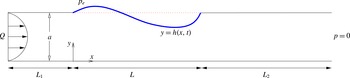
We consider the two-dimensional flow of an incompressible Newtonian fluid of density
 $\unicode[STIX]{x1D70C}$
and viscosity
 $\unicode[STIX]{x1D707}$
through a long (planar) rigid channel of constant width
 $a$
and total length
 $L_{0}$
. A segment of length
 $L$
of one wall of this channel is replaced by a massless membrane with constant longitudinal tension
 $T_{0}$
, forming an upstream rigid segment of length
 $L_{1}$
and a downstream rigid segment of length
 $L_{2}$
either side of the compliant segment. We measure lengths along the entirely rigid wall by the coordinate
 $x$
, where
 $x=0$
is the intersection between the upstream rigid segment and the flexible membrane. Similarly, we measure perpendicular displacements from the rigid wall by the coordinate
 $y$
, where the position of the flexible wall is denoted as
 $y=h(x,t)$
across
 $0\leqslant x\leqslant L$
. The model set-up is shown in figure 1.
Set-up of the model in dimensionless variables.

Flow along the channel with velocity
 $\boldsymbol{u}=(u,v)$
and pressure
 $p$
satisfies the two-dimensional Navier–Stokes equations, driven by a fixed flux
 $Q$
(per unit width in the out-of-plane direction) at the upstream end and a fixed pressure
 $P_{0}$
at the downstream end. Furthermore, we impose a constant external pressure
 $P_{e}$
on the flexible membrane. Neglecting normal viscous stresses (which are typically small for the parameters considered below), a normal stress balance on the wall takes the form
 $$\begin{eqnarray}p=P_{e}-T_{0}\unicode[STIX]{x1D705}(h),\quad (y=h),\end{eqnarray}$$
where
 $\unicode[STIX]{x1D705}(h)$
represents the curvature of the elastic interface
 $y=h(x,t)$
(see for example Jensen & Heil Reference Jensen and Heil2003; Stewart et al.
Reference Stewart, Waters and Jensen2009).
We adopt a long-wavelength approach by rescaling the variables according to
 $$\begin{eqnarray}x=L\hat{\hat{x}},\quad y=a\hat{{\hat{y}}},\quad u=(Q/a)\hat{\hat{u} },\quad v=(Q/L)\hat{\hat{v}},\quad p=P_{0}+\unicode[STIX]{x1D70C}(Q^{2}/a^{2})\hat{\hat{p}},\end{eqnarray}$$
where variables with a double hat are assumed
 $O(1)$
, resulting in the following dimensionless groups
 $$\begin{eqnarray}R=\frac{\unicode[STIX]{x1D70C}Q}{\unicode[STIX]{x1D707}},\quad p_{e}=\frac{a^{2}(P_{e}-P_{0})}{\unicode[STIX]{x1D70C}Q^{2}},\quad T=\frac{aT_{0}}{Q^{2}},\quad \hat{\hat{L}}_{1}=\frac{L_{1}}{a},\quad \hat{\hat{L}}_{2}=\frac{L_{2}}{a},\end{eqnarray}$$
denoting the Reynolds number, the dimensionless external pressure, the dimensionless membrane tension and the dimensionless lengths of the upstream and downstream segments, respectively. We henceforth drop double hats for notational convenience.
Neglecting terms of
 $O(a^{2}/L^{2})$
, the flow satisfies the long-wavelength (dimensionless) Navier–Stokes equations, in the form
 $$\begin{eqnarray}\displaystyle & \displaystyle u_{x}+v_{y}=0, & \displaystyle\end{eqnarray}$$
 $$\begin{eqnarray}\displaystyle & \displaystyle u_{t}+uu_{x}+vu_{y}=-p_{x}+\frac{1}{R}u_{yy}, & \displaystyle\end{eqnarray}$$
 $$\begin{eqnarray}\displaystyle & \displaystyle p_{y}=0, & \displaystyle\end{eqnarray}$$
subject to boundary conditions of no-slip along the rigid segments of the channel walls,
 $u=v=0$
; along the flexible membrane the flow is subject to no-slip and kinematic conditions in the form
 $$\begin{eqnarray}u=0,\quad v=h_{t},\quad (y=h),\end{eqnarray}$$
as well as continuity of normal stress (dimensionless, long-wavelength version of (2.1)),
 $$\begin{eqnarray}p=p_{e}-Th_{xx},\quad (y=h).\end{eqnarray}$$
To allow analytical progress, we reduce the governing equations to a one-dimensional system in a similar manner to other studies of collapsible channel flow (Stewart et al.
Reference Stewart, Waters and Jensen2009, Reference Stewart, Heil, Waters and Jensen2010; Xu et al.
Reference Xu, Billingham and Jensen2013, Reference Xu, Billingham and Jensen2014); this reduction is described in detail by Stewart et al. (Reference Stewart, Waters and Jensen2009). In summary, since
 $p$
is independent of
 $y$
through (2.4c
), we integrate (2.4a
) and (2.4b
) across the channel width and close the resulting system of equations using a von Karman–Pohlhausen flow profile assumption, where we set
 $$\begin{eqnarray}u=\frac{6qy(h-y)}{h^{3}},\quad q=\int _{0}^{h}u\,\text{d}y,\end{eqnarray}$$
where
 $q$
is a flux per unit width in the out-of-plane direction. Although not strictly rational, predictions of similar models using these flow profile assumptions show encouraging agreement with full numerical simulations of the same system (Stewart et al.
Reference Stewart, Heil, Waters and Jensen2010; Xu et al.
Reference Xu, Billingham and Jensen2014).
Since the pressure does not vary in the cross-stream direction (2.4c
), in the compliant segment of the channel (
 $0\leqslant x\leqslant 1$
) the fluid pressure follows directly from the normal stress boundary condition (2.4e
). Conversely, in the rigid segments of the channel, where the fluid flux is spatially uniform (
 $h=1$
,
 $q_{x}=0$
), the fluid pressure varies linearly in
 $x$
through (2.4b
). For the upstream rigid segment (
 $-L_{1}\leqslant x\leqslant 0$
) the inlet flux condition dictates that
 $q=1$
everywhere, forming a boundary condition for the compliant segment while the corresponding upstream driving pressure follows as
 $$\begin{eqnarray}p_{u}(t)=p(-L_{1},t)=p_{e}+\frac{12L_{1}}{R}-Th_{xx}(0,t).\end{eqnarray}$$
However, since the flux is constant, consideration of flow in this segment is unnecessary and the parameter
 $L_{1}$
can be set to zero without loss of generality (in agreement with Xu et al. (Reference Xu, Billingham and Jensen2013, Reference Xu, Billingham and Jensen2014)).
In the downstream rigid segment (
 $1\leqslant x\leqslant 1+L_{2}$
) the
 $x$
-momentum equation can be rearranged to solve for the fluid pressure profile subject to the compatibility constraint
 $$\begin{eqnarray}Th_{xx}=p_{e}-L_{2}\left[\frac{12q}{R}+q_{t}\right],\quad (x=1),\end{eqnarray}$$
which forms a boundary condition on the flow in the compliant segment. The system is closed by imposing that the membrane remains pinned at its ends, so that
 $h(0)=h(1)=1$
.
Hence, the governing equations can be summarised as
 $$\begin{eqnarray}h_{t}+q_{x}=0,\quad q_{t}+\frac{6}{5}\left(\frac{q^{2}}{h}\right)_{x}=Thh_{xxx}-\frac{12}{R}\frac{q}{h^{2}},\end{eqnarray}$$
subject to boundary conditions
 $$\begin{eqnarray}h=1,\quad q=1,\quad (x=0),\end{eqnarray}$$
 $$\begin{eqnarray}h=1,\quad Th_{xx}=p_{e}-L_{2}\left(\frac{12}{R}q+q_{t}\right),\quad (x=1),\end{eqnarray}$$
which forms a closed system. These governing equations are similar to those derived by Xu et al. (Reference Xu, Billingham and Jensen2013, Reference Xu, Billingham and Jensen2014), although here we consider a constant external pressure as opposed to an external pressure gradient, which modifies (2.8b,d ).
This system includes all the essential ingredients for predicting the onset of self-excited oscillations (fluid inertia, a source of dissipation, wall elasticity) and can be solved with much reduced computational cost compared to the full two-dimensional system. This model (2.8) converges to the full two-dimensional (long-wavelength) system in the limit as
 $R\rightarrow 0$
(cf. lubrication theory). For
 $R>0$
, use of the von Karman–Pohlhausen flow approximation means that this model is not entirely rational, but it remains a paradigmatic example whose behaviour can be used to better understand some aspects of what can be found in the two-dimensional system. For example, versions of these equations with an external pressure gradient (Stewart et al.
Reference Stewart, Waters and Jensen2009) have been able to replicate many of the features of the ‘sloshing’ oscillations found in the two-dimensional system by Jensen & Heil (Reference Jensen and Heil2003) driven by fixed upstream pressure in the limit of large
 $T$
. In addition, Xu et al. (Reference Xu, Billingham and Jensen2014) showed that these equations (again with an external pressure gradient) predicted a new family of ‘sawtooth’ oscillations driven by fixed upstream flux, which were also present in full two-dimensional simulations. Finally, Stewart et al. (Reference Stewart, Heil, Waters and Jensen2010) showed that these equations predict highly nonlinear ‘slamming’ oscillations (discussed below) in some regions of parameter space, in strong qualitative agreement with full two-dimensional computations.
2.1 Static solutions
Static solutions to (2.8) must have unit flux to satisfy the inlet flow condition, while the corresponding membrane profile
 $h=h^{(s)}(x)$
must satisfy the third-order nonlinear ordinary differential equation (ODE)
 $$\begin{eqnarray}\frac{6}{5}\left(\frac{1}{h^{(s)}}\right)_{x}=Th^{(s)}h_{xxx}^{(s)}-\frac{12}{R}\frac{1}{(h^{(s)})^{2}},\quad (0\leqslant x\leqslant 1),\end{eqnarray}$$
subject to three boundary conditions
 $$\begin{eqnarray}\displaystyle & \displaystyle h^{(s)}=1,\quad (x=0), & \displaystyle\end{eqnarray}$$
 $$\begin{eqnarray}\displaystyle & \displaystyle h^{(s)}=1,\quad Th_{xx}^{(s)}=p_{e}-\frac{12L_{2}}{R},\quad (x=1). & \displaystyle\end{eqnarray}$$
The superscript
 $(s)$
has been used throughout to denote the static solution and
 $p^{(s)}(x)$
denotes the corresponding static pressure profile. Following Stewart et al. (Reference Stewart, Waters and Jensen2009), these equations can be discretised using finite differences and solved numerically using Newton’s method. Static solutions to (2.9) are described in § 3. In a similar manner to Xu et al. (Reference Xu, Billingham and Jensen2013), it is also instructive to consider inviscid static solutions, discussed in appendix A. Throughout this paper we consider relatively large external pressures where the channel is collapsed for a region along its length, and we typically characterise the static solutions using the maximal channel constriction
 $h_{m}^{(s)}=\min _{x}(h^{(s)})$
with corresponding
 $x$
position
 $x_{m}^{(s)}$
.
2.2 Linear stability global eigensolver
We consider the stability of a static solution of (2.9) by considering the growth of a small perturbation to this state, writing
 $$\begin{eqnarray}(h,q)=(h^{(s)}(x),1)+\unicode[STIX]{x1D703}[(\tilde{h}(x),\tilde{q}(x))\text{e}^{\unicode[STIX]{x1D70E}t}+(\tilde{h}^{\ast }(x),\tilde{q}^{\ast }(x))\text{e}^{\unicode[STIX]{x1D70E}^{\ast }t}],\quad (0\leqslant x\leqslant 1),\end{eqnarray}$$
where
 $\unicode[STIX]{x1D703}\ll 1$
and
 $\tilde{h}(x;\unicode[STIX]{x1D70E})$
and
 $\tilde{q}(x;\unicode[STIX]{x1D70E})$
are functions of
 $x$
and
 $^{\ast }$
denotes a complex conjugate. Substituting into the full governing equations (2.8) and neglecting terms of
 $O(\unicode[STIX]{x1D703}^{2})$
we obtain the linearised equations
 $$\begin{eqnarray}\displaystyle & \displaystyle \unicode[STIX]{x1D70E}\tilde{h}+\tilde{q}_{x}=0, & \displaystyle\end{eqnarray}$$
 $$\begin{eqnarray}\displaystyle & \displaystyle \unicode[STIX]{x1D70E}\tilde{q}+\frac{6}{5}\left(\frac{2\tilde{q}}{h^{(s)}}-\frac{\tilde{h}}{(h^{(s)})^{2}}\right)_{x}=Th^{(s)}\tilde{h}_{xxx}+T\tilde{h}h_{xxx}^{(s)}-\frac{12}{R}\left(\frac{\tilde{q}}{(h^{(s)})^{2}}-\frac{2\tilde{h}}{(h^{(s)})^{3}}\right),\hspace{12.0pt} & \displaystyle\end{eqnarray}$$
subject to linearised boundary conditions
 $$\begin{eqnarray}\displaystyle & \displaystyle \tilde{h}=0,\quad \tilde{q}=0,\quad (x=0), & \displaystyle\end{eqnarray}$$
 $$\begin{eqnarray}\displaystyle & \displaystyle \tilde{h}=0,\quad T\tilde{h}_{xx}=-L_{2}\left(\frac{12}{R}\tilde{q}+\unicode[STIX]{x1D70E}\tilde{q}\right),\quad (x=1). & \displaystyle\end{eqnarray}$$
Equations (2.11) constitute a global eigenvalue problem for
 $\unicode[STIX]{x1D70E}$
and the corresponding eigenfunctions
 $\tilde{q}(x;\unicode[STIX]{x1D70E})$
and
 $\tilde{h}(x;\unicode[STIX]{x1D70E})$
, which must be solved numerically. To form a solution to the eigenvalue problem (2.11) we construct a global eigensolver by discretising the collapsible segment of the channel
 $x$
onto a uniform mesh
 $x_{j}=j\unicode[STIX]{x0394}x$
(
 $j=0,\ldots ,N-1$
), where
 $\unicode[STIX]{x0394}x=1/(N-1)$
. We then discretise the perturbation eigenfunctions onto this mesh by writing
 $\tilde{h}_{j}=\tilde{h}(x_{j};\unicode[STIX]{x1D70E})$
and
 $\tilde{q}_{j}=\tilde{q}(x_{j};\unicode[STIX]{x1D70E})$
(
 $j=0,\ldots ,N-1$
) and form the vector of unknown coefficients
 $\boldsymbol{a}=[\tilde{h}_{0},\ldots ,\tilde{h}_{N-1},\tilde{q}_{0},\ldots ,\tilde{q}_{N-1}]^{\text{T}}$
. By expressing spatial derivatives using second-order centred finite difference approximations, we hence express (2.11) as an eigenvalue problem in the form
 $$\begin{eqnarray}\unicode[STIX]{x1D648}\boldsymbol{a}=\unicode[STIX]{x1D70E}\boldsymbol{a},\end{eqnarray}$$
where
 $\unicode[STIX]{x1D648}$
is a matrix of size
 $2N\times 2N$
. The eigenvalues (
 $\unicode[STIX]{x1D70E}$
) and corresponding eigenvectors (
 $\boldsymbol{a}$
) can be calculated numerically using Matlab in a straightforward manner. For computation of the energy budget below we normalise the eigenfunction so that
 $\max (\text{Re}(\tilde{q}(x;\unicode[STIX]{x1D70E})))=1$
unless specified otherwise. Results of the linear stability analysis are described in §§ 4.1–4.2. In simulations we use up to a maximum of
 $N=1600$
grid points to resolve the highly constricted static shape and associated eigenfunctions. Simulations for larger
 $N$
became impractical and were not deemed necessary. This global eigensolver is similar in spirit to that constructed by Luo et al. (Reference Luo, Cai, Li and Pedley2008) (see also Liu et al. (Reference Liu, Luo, Cai and Pedley2009, Reference Liu, Luo and Cai2012)) using a finite element method and an Arnoldi algorithm for computing eigenvalues, but their two-dimensional eigensolver requires extremely large matrices and is impractical for large-scale parameter sweeps. Since the present approach is one-dimensional it has the advantage of much reduced computational cost permitting a unified overview of the parameter space.
2.3 Fully nonlinear simulations
Nonlinear, time-dependent simulations of (2.8) can be constructed using the semi-implicit finite difference method described and used previously by Stewart et al. (Reference Stewart, Waters and Jensen2009). In particular, we discretise spatial derivatives using fourth-order finite differences and time derivatives using first-order finite differences, representing the highest spatial derivative in each equation implicitly with all other terms treated explicitly. To capture the highly complicated ‘slamming’ oscillations described below we use an increased temporal and spatial grid in regions where the membrane gets drawn close to the rigid wall. We have also thoroughly checked for convergence of the scheme using a variety of spatial and temporal grids up to a maximum of 3000 equally spaced spatial grid points. Results of the fully nonlinear simulations are described in § 7. We typically characterise the numerical simulations by considering the temporal evolution of the maximal channel constriction
 $h_{m}(t)=\min _{x}(h(x,t))$
.
2.4 Energy budget
Following Stewart et al. (Reference Stewart, Waters and Jensen2009), we compute the corresponding energy budget for the flow by multiplying (2.8) by
 $6q/(5h)$
and integrating over the channel length and width. This energy budget can be written in the form
 $$\begin{eqnarray}{\mathcal{K}}+{\mathcal{E}}={\mathcal{F}}+{\mathcal{P}}-{\mathcal{D}}_{S}-{\mathcal{D}}_{A},\end{eqnarray}$$
where
 $$\begin{eqnarray}\displaystyle & \displaystyle {\mathcal{K}}=\frac{3}{5}\frac{\unicode[STIX]{x2202}}{\unicode[STIX]{x2202}t}\left(\int _{0}^{1}\frac{q^{2}}{h}\,\text{d}x+\int _{-L_{1}}^{0}q^{2}\,\text{d}x+\int _{1}^{1+L_{2}}q^{2}\,\text{d}x\right), & \displaystyle\end{eqnarray}$$
 $$\begin{eqnarray}\displaystyle & \displaystyle {\mathcal{F}}=-\frac{18}{25}\left[\frac{q^{3}}{h^{2}}\right]_{x=0}^{x=1}, & \displaystyle\end{eqnarray}$$
 $$\begin{eqnarray}\displaystyle & \displaystyle {\mathcal{P}}=\frac{6}{5}p_{u}=\frac{6}{5}\left(p_{e}+\frac{12L_{1}}{R}-Th_{xx}(0,t)\right), & \displaystyle\end{eqnarray}$$
 $$\begin{eqnarray}\displaystyle & \displaystyle {\mathcal{E}}=\frac{6}{5}\frac{\unicode[STIX]{x2202}}{\unicode[STIX]{x2202}t}\left(\int _{0}^{1}\left(p_{e}h+\frac{1}{2}Th_{x}^{2}\right)\,\text{d}x\right), & \displaystyle\end{eqnarray}$$
 $$\begin{eqnarray}\displaystyle & \displaystyle {\mathcal{D}}_{S}=\frac{72}{5R}\left(\int _{0}^{1}\frac{q^{2}}{h^{3}}\,\text{d}x+\int _{-L_{1}}^{0}q^{2}\,\text{d}x+\int _{1}^{1+L_{2}}q^{2}\,\text{d}x\right), & \displaystyle\end{eqnarray}$$
 $$\begin{eqnarray}\displaystyle & \displaystyle {\mathcal{D}}_{A}=\frac{3}{25}\int _{0}^{1}\frac{q^{2}q_{x}}{h^{2}}\,\text{d}x, & \displaystyle\end{eqnarray}$$
where
 ${\mathcal{K}}$
measures the rate of change of kinetic energy,
 ${\mathcal{F}}$
is the net kinetic energy flux extracted from the mean flow,
 ${\mathcal{P}}$
is the rate of working of upstream pressure forces,
 ${\mathcal{E}}$
is the rate of working of pressure forces across the membrane,
 ${\mathcal{D}}_{S}$
is the rate of working of viscous forces and
 ${\mathcal{D}}_{A}$
is the additional kinetic energy flux induced by the flow profile assumption. The terms in the fully nonlinear energy budget for periodic oscillations are computed in § 7.3. It should be noted that
 ${\mathcal{P}}$
is proportional to the upstream pressure
 $p_{u}$
, which can in turn be expressed in terms of the external pressure on the membrane and the membrane curvature at the upstream end of the flexible segment.
2.5 Energy budget for static solutions
For a static membrane (described in § 2.1) the only non-trivial contributions to the energy budget can be expressed as (steady components denoted with a superscript
 $(s)$
),
 $$\begin{eqnarray}{\mathcal{P}}^{(s)}={\mathcal{D}}^{(s)},\end{eqnarray}$$
where
 $$\begin{eqnarray}\displaystyle & \displaystyle {\mathcal{D}}^{(s)}=\frac{72}{5R}\left(\int _{0}^{1}\frac{1}{(h^{(s)})^{3}}\,\text{d}x+L_{1}+L_{2}\right), & \displaystyle\end{eqnarray}$$
 $$\begin{eqnarray}\displaystyle & \displaystyle {\mathcal{P}}^{(s)}=\frac{6}{5}\left(p_{e}+\frac{12L_{1}}{R}-Th_{xx}^{(s)}(0)\right). & \displaystyle\end{eqnarray}$$
Using the downstream boundary condition (2.9c ) this static energy balance can be rewritten as
 $$\begin{eqnarray}T[h_{xx}^{(s)}]_{0}^{1}=\frac{12}{R}\int _{0}^{1}\frac{1}{(h^{(s)})^{3}}\,\text{d}x;\end{eqnarray}$$
this relation is employed to close the reduced system of equations constructed in the limit of large
 $p_{e}$
in § 6.
2.6 Rate of working of viscous dissipation
To elucidate the energy budget of neutrally stable oscillations, we consider the rate of working of viscous forces (2.13f
) in more detail. In particular, we consider the time average over a period of oscillation, denoted by an overbar. We consider the perturbation expansion posed in (2.10) continued to the next order in
 $\unicode[STIX]{x1D703}$
in the form
 $$\begin{eqnarray}\displaystyle (h,q) & = & \displaystyle (h^{(s)},1)+\unicode[STIX]{x1D703}[(\tilde{h},\tilde{q})\text{e}^{\unicode[STIX]{x1D70E}t}+(\tilde{h}^{\ast },\tilde{q}^{\ast })\text{e}^{\unicode[STIX]{x1D70E}^{\ast }t}]\nonumber\\ \displaystyle & & \displaystyle +\,\unicode[STIX]{x1D703}^{2}[(\check{h},\check{q})\text{e}^{2\unicode[STIX]{x1D70E}t}+(\overline{\check{h}},\overline{\check{q}})+(\check{h}^{\ast },\check{q}^{\ast })\text{e}^{2\unicode[STIX]{x1D70E}^{\ast }t}]+O(\unicode[STIX]{x1D703}^{3}).\end{eqnarray}$$
Using this expansion we approximate
 ${\mathcal{D}}_{S}$
(2.13f
) by expanding in powers of
 $\unicode[STIX]{x1D703}$
. At leading order
 $\overline{{\mathcal{D}}_{S}}={\mathcal{D}}_{S}^{(s)}$
. At the following order, the variables have components which are proportional to either
 $\exp (\unicode[STIX]{x1D70E}t)$
or
 $\exp (\unicode[STIX]{x1D70E}^{\ast }t)$
, so taking the time average over a period of neutrally stable oscillation (
 $\text{Re}(\unicode[STIX]{x1D70E})=0$
) implies that the
 $O(\unicode[STIX]{x1D703})$
contribution to
 $\overline{{\mathcal{D}}_{S}}$
must be zero. Conversely, at
 $O(\unicode[STIX]{x1D703}^{2})$
, the checked variables consist of time-independent terms (denoted as
 $\overline{\check{h}}$
and
 $\overline{\check{q}}$
for
 $h$
and
 $q$
, respectively) as well as time-dependent components which are proportional to either
 $\exp (2\unicode[STIX]{x1D70E}t)$
or
 $\exp (2\unicode[STIX]{x1D70E}^{\ast }t)$
. Hence, when averaging over a period of neutrally stable oscillation, we obtain a non-trivial contribution to the energy budget at
 $O(\unicode[STIX]{x1D703}^{2})$
. A similar approach was previously considered by Stewart et al. (Reference Stewart, Heil, Waters and Jensen2010) to compute the perturbation energy budget of ‘sloshing’ oscillations driven by fixed upstream pressure.
Hence, we expand the time-averaged rate of working of viscous dissipation in the form
 $$\begin{eqnarray}\overline{{\mathcal{D}}_{S}}={\mathcal{D}}_{S}^{(s)}+\unicode[STIX]{x1D703}^{2}(\overline{\tilde{{\mathcal{D}}}_{S}}+\overline{\check{{\mathcal{D}}}_{S}})+O(\unicode[STIX]{x1D703}^{3}),\end{eqnarray}$$
where
 $$\begin{eqnarray}\overline{\tilde{{\mathcal{D}}}_{S}}=\frac{144}{5R}\left(\int _{0}^{1}\frac{6\tilde{h}\tilde{h}^{\ast }-3h^{(s)}\tilde{h}^{\ast }\tilde{q}-3h^{(s)}\tilde{h}\tilde{q}^{\ast }+(h^{(s)})^{2}\tilde{q}\tilde{q}^{\ast }}{(h^{(s)})^{5}}\,\text{d}x+L_{2}\tilde{q}(1)\tilde{q}^{\ast }(1)\right),\end{eqnarray}$$
consists of terms which involve the eigenfunctions
 $\tilde{h}$
and
 $\tilde{q}$
(and their complex conjugates) determined above, while
 $$\begin{eqnarray}\overline{\check{{\mathcal{D}}}_{S}}=\frac{72}{5R}\int _{0}^{1}\frac{-3\overline{\check{h}}}{(h^{(s)})^{4}}\,\text{d}x\end{eqnarray}$$
consists only of time-independent terms arising at second order in
 $\unicode[STIX]{x1D703}$
. We note that
 $\overline{\check{q}}$
must be zero to satisfy conservation of mass over a period of neutrally stable oscillation, so
 $\overline{\check{{\mathcal{D}}}_{S}}$
depends on
 $\overline{\check{h}}$
alone. The quantity
 $\overline{\tilde{{\mathcal{D}}}}_{S}$
can be easily computed from eigenfunctions obtained from the global stability eigensolver discussed in § 2.2. However, solution of the
 $O(\unicode[STIX]{x1D703}^{2})$
perturbation problem would be required to compute
 $\overline{\check{{\mathcal{D}}}_{S}}$
, which is not considered here. We use this decomposition of
 $\overline{{\mathcal{D}}_{S}}$
in § 7.3 to elucidate the mechanism of energy transfer sustaining the self-excited oscillations.
3 Static membrane profiles
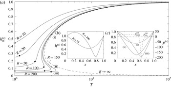
In this section we consider nonlinear static solutions of (2.9), summarised in figure 2. In particular, we consider a parametric plot of the minimal channel width (
 $h_{m}^{(s)}\leqslant 1$
) as a function of the membrane tension
 $T$
for several values of the Reynolds number
 $R$
for fixed external pressure
 $p_{e}=10$
and downstream length
 $L_{2}=3$
(figure 2
a). Corresponding static membrane profiles for
 $T=1$
are shown for both
 $R=10$
and
 $R=100$
in figure 2(b) (at the points labelled with open circles in figure 2
a). Similarly, the three possible static membrane profiles for
 $T=3$
and
 $R=200$
are shown in figure 2(c) (at the points labelled with crosses in figure 2
a). For low tensions the channel is highly constricted at one point along its length due to the collapsing influence of the external pressure (figure 2
b). This collapse is further exaggerated by the Bernoulli effect as the Reynolds number increases (figure 2
b). This state is similar to the highly collapsed membrane profiles reported by Xu & Jensen (Reference Xu and Jensen2015). As the membrane tension increases the channel gradually becomes less collapsed, approaching a state where the channel is close to uniform along its length, similar to the uniform state admissible with an external pressure gradient (Xu et al.
Reference Xu, Billingham and Jensen2013). For low Reynolds numbers the transition between the highly collapsed and uniform states is monotonic (see curves for
 $R=10$
,
 $R=50$
in figure 2
a). However, beyond a critical Reynolds number
 $R_{b}$
the trace of the maximal channel constriction becomes multi-valued for a range of membrane tension, exhibiting three static states for a given
 $T$
(see curves for
 $R=100$
and greater in figure 2
a). The highly collapsed static state and the almost uniform static state are both stable to (static) perturbations, while the intermediate state is unstable. The change in stability occurs through two limit-point (or saddle-node) bifurcations, one at each end the intermediate branch. The path of these limit points in parameter space is also shown as dotted lines in figures 4(a,b) and 10(a). Also, in figure 4(b) we illustrate the regions of the parameter space where two stable static solutions coexist (dark shaded region). The corresponding trace of the inviscid static state (discussed in appendix A) is also shown in figure 2(a) (dashed line), where the system exhibits a single limit-point (saddle-node) bifurcation at
 $T=T_{c}$
(
 $T_{c}\approx 2.426$
for
 $p_{e}=10$
), with two branches of static solutions for
 $T>T_{c}$
, where the upper branch is stable and the lower branch unstable. These branches are analogous to the almost uniform and the intermediate branches identified for finite
 $R$
. However, the highly collapsed static state for finite
 $R$
does not exist in the inviscid limit, as this is maintained by viscous effects (see § 6).
An example of the multiple static states at the same point in parameter space is shown in figure 2(c) for
 $T=3$
and
 $R=200$
. These profiles are labelled (i)–(iii), where (i) is the most inflated profile and (iii) is the most constricted. Both (i) and (iii) are stable to (static) perturbations. This existence of multiple stable static states is reminiscent of the work of Reyn (Reference Reyn1987) and consistent with examples of ‘flow limitation’ or ‘choking’ (Luo & Pedley Reference Luo and Pedley2000; Stewart Reference Stewart2010). Furthermore, there is a sharp contrast between the pressure profiles of these two (stable) static configurations, also shown in figure 2(c). The pressure corresponding to profile (i) (dot-dashed line in figure 2
c) exhibits only small variations along the collapsible segment. Conversely, the pressure corresponding to profile (iii) (dashed line in figure 2
c) is approximately piecewise constant with a decrease across the point of maximal constriction (due to viscous effects) with a significant overshoot due to the Bernoulli effect (the pressure required to maintain the rapid flow through the constriction). Siviglia & Toffolon (Reference Siviglia and Toffolon2014) analysed a one-dimensional model of flow in a long collapsible tube in the absence of membrane tension, showing that a localised change in the properties of the wall (mimicking our compliant segment of the channel) can induce multiple stable states, one supercritical and another which exhibits an elastic jump (and hence sharp changes in pressure), similar to the experiments of Kececioglu et al. (Reference Kececioglu, Mcclurken, Kamm and Shapiro1981). Our profiles (i) and (iii) are significantly different from each other, in agreement with Siviglia and Toffolon’s results, but given the dispersive nature of the current one-dimensional model it is not clear if profile (iii) is transcritical.
Nonlinear static solutions of the model for prescribed upstream flux: (a) plot of the maximal channel constriction as a function of the wall tension for
 $R=10$
,
 $R=50$
,
 $R=100$
,
 $R=150$
and
 $R=200$
; (b) the unique static wall profiles for
 $T=1$
and both
 $R=10$
and
 $R=100$
(points marked with open circles on a); (c) the three static walls profile for
 $T=3$
and
 $R=200$
at the points (i)–(iii) marked with crosses on (a) (left-hand axis) while the corresponding static pressure profiles in (i) and (iii) are shown as a dot-dashed and dashed lines, respectively (right-hand axis). Here
 $p_{e}=10$
and
 $L_{2}=3$
. The dashed line in (a) is the inviscid static state. The filled circles in (a) indicate the critical value of the membrane tension below which the static branch is unstable to oscillations.

4 Linear stability of the static membrane profiles
In this section we consider the stability of the nonlinear static profiles constructed in § 3, examining the structure of a typical global eigenvalue spectrum (§ 4.1) and isolating neutrally stable oscillatory modes (§ 4.2).
4.1 Typical eigenvalue spectra
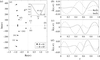
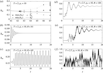
Having characterised the static membrane profiles, we now use the global eigensolver described in § 2.2 to consider their stability to time-dependent perturbations. Two typical eigenvalue spectra are plotted in figure 3(a), plotting
 $\text{Re}(\unicode[STIX]{x1D70E})$
against
 $\text{Im}(\unicode[STIX]{x1D70E})$
for the static state plotted in the inset. Eigenvalues appear as complex conjugate pairs, which are all stable (
 $\text{Re}(\unicode[STIX]{x1D70E})<0$
) for sufficiently small Reynolds numbers. As the Reynolds number increases a pair of eigenvalues will cross the
 $\text{Re}(\unicode[STIX]{x1D70E})$
axis with non-zero imaginary part, indicative of a Hopf bifurcation. Two cases are illustrated for
 $T=2$
,
 $p_{e}=10$
and
 $L_{2}=3$
in figure 3(a):
 $R=61$
, where all eigenvalues are stable (filled black circles), and
 $R=65$
, where two conjugate pairs of eigenvalues are unstable (crosses). In figure 3(b–d) we plot the corresponding eigenfunctions
 $\tilde{h}(x;\unicode[STIX]{x1D70E})$
of the three most unstable modes for
 $R=65$
; the structure of these eigenfunctions is explained in more detail below.
(a) Eigenvalue spectra for
 $T=2$
,
 $p_{e}=10$
and
 $L_{2}=3$
, with
 $R=61$
(filled circles) and
 $R=65$
(crosses). The pairs of modes are labelled (i)–(vi) in order of increasing stability. Inset shows the corresponding static shape of the wall for
 $R=61$
(dashed) and
 $R=65$
(solid). Corresponding eigenfunctions
 $\tilde{h}(x;\unicode[STIX]{x1D70E})$
of the three most unstable modes for
 $R=65$
: (b) mode (i); (c) mode (ii); (d) mode (iii). Eigenfunctions have been normalised so that
 $\max (\text{Re}(\tilde{q}))=1$
. The dotted line in (b–d) denotes the position
 $x_{m}^{(s)}$
.

4.2 Neutrally stable oscillations
Neutral stability curves (along which
 $\text{Re}(\unicode[STIX]{x1D70E})=0$
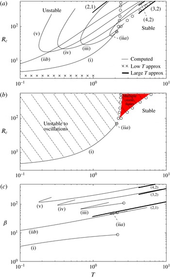
) in the parameter space spanned by the membrane tension and critical Reynolds number are shown in figure 4(a) for
 $p_{e}=10$
and
 $L_{2}=3$
. In particular, we illustrate the neutral stability curves for the five most unstable modes identified in the spectrum in figure 3. These modes are labelled (i) to (v). We have verified that for these parameter values the primary global instability of the system is always either to the mode labelled (i) or (iia). It should be noted that the mode labelled (ii) becomes unstable in two separate regions across the parameter space, labelled (iia) and (iib), respectively. Interestingly, the neutral curve for mode (iib) exhibits a low-frequency oscillation for low tensions (consistent with the framework described in § 5) but a high-frequency oscillation for large tensions (consistent with the framework described in § 6). Although these neutral curves intersect one another, they do so with distinct frequencies, so there is no mode interaction. In addition, in figure 4(b) we illustrate regions of parameter space where the system is unstable to oscillations using hatching, as well as highlighting the corresponding regions of parameter space where multiple steady states exist (dark shaded region). The corresponding oscillation frequency of each mode is shown in figure 4(c); for each mode the oscillation frequency increases with membrane tension, which is exploited in § 6.
Previous studies of collapsible channel flow (e.g. Luo et al.
Reference Luo, Cai, Li and Pedley2008; Stewart et al.
Reference Stewart, Waters and Jensen2009) characterise these modes by the number of turning points in the eigenfunction of the membrane shape,
 $\tilde{h}(x;\unicode[STIX]{x1D70E})$
. Hence, according to this convention for
 $T=2$
the mode labelled (i) would be mode-4, the mode labelled (iia) would be mode-5 and the mode labelled (iii) would be mode-6. However, for lower tensions the mode labelled (i) has two extrema (see figure 7
a) and is thus mode-2, so the shape of the eigenfunction changes along the neutral curve. In this study it emerges that for large tensions a more convenient labelling convention is to characterise the eigenfunction relative to the point of greatest channel constriction,
 $x_{m}^{(s)}$
(position denoted with a dotted line on the panels in figure 3
b–d). We characterise the eigenfunctions of neutrally stable modes in more detail using the asymptotic model of § 6.
Neutrally stable modes for
 $p_{e}=10$
and
 $L_{2}=3$
as a function of the membrane tension
 $T$
: (a) the critical value of the Reynolds number for instability of the six most unstable modes labelled (i) to (v); (b) regions of the
 $(T,R)$
parameter space where the system has multiple coexisting static states (dark shaded region) and regions where the highly collapsed basic state is unstable to oscillations (hatching); (c) corresponding frequency of the neutrally stable modes. The open circles in (a) correspond to limit (saddle) points associated with a change in the number of static configurations, while the crosses represent the leading-order prediction for the critical Reynolds number from the low-frequency theory in § 5. The labels
 $(m,n)$
follow from the asymptotic description of the eigenfunction of the wall shape in the limit of large
 $T$
described in § 6, where
 $m$
is the number of turning points upstream of the constriction and
 $n$
is the number of turning points downstream.

It is also instructive to consider the onset of instability in terms of the corresponding static configuration of the membrane. In figure 2(a) we indicate with a filled circle the critical value of the membrane tension below which each branch of static solutions becomes unstable to self-excited oscillations. For this value of the external pressure, configurations approaching the uniform state (along the upper branch as
 $T\rightarrow \infty$
) are always stable for large tensions. This is consistent with the study of Xu et al. (Reference Xu, Billingham and Jensen2013), who found that the uniform static configuration (maintained with an external pressure gradient) is always stable beyond a critical value of the membrane tension
 $T\approx 0.121$
.
Of most pertinent interest in the system is the first onset of self-excited oscillations, termed the primary oscillatory instability. For increasing
 $T$
, the system exhibits three distinct behaviours. Each of these is now discussed in turn.
4.2.1 Primary oscillatory instability for low membrane tensions
For sufficiently low membrane tensions the primary oscillatory instability of the system is via the mode labelled (i), as shown in figure 4. The neutral curve for this branch extends as
 $T\rightarrow 0$
(a singular limit) where the critical Reynolds number approaches a constant. The eigenfunction for
 $\tilde{h}$
has two extrema for
 $T=0.1$
and is thus mode-2 (see also plots for
 $T=0.01$
in figure 7
c). The corresponding shape of the static membrane and perturbation eigenfunction as well as the critical Reynolds number required for the onset of instability are explored in the limit as
 $p_{e}\rightarrow \infty$
in § 5 and appendix C. For larger Reynolds numbers the system admits a secondary instability of the static shape with neutral curve labelled (iib), which again persists as
 $T\rightarrow 0$
, where the eigenfunction for
 $\tilde{h}$
has three extrema for
 $T=0.1$
and is thus mode-3. We further explore this family of oscillations in the limit as
 $T\rightarrow 0$
in § 5, where we hypothesise that these are the first two branches of an infinite family of low-frequency oscillatory modes. The nonlinear growth of oscillations along the branch (i) is explored in § 7.1, while the corresponding energy budget of the fully developed oscillations is explored in § 7.3.
4.2.2 Primary global instability for intermediate membrane tensions
For intermediate membrane tensions the primary oscillatory instability of the system is via the high-frequency mode labelled (iia). In this case the neutral curve does not persist to low tensions and instead takes the form of a tongue (figure 4) with an upper and lower branch (similar to other phenomena in hydrodynamic stability theory, such as the onset of Tollmien–Schlichting waves (Drazin & Reid Reference Drazin and Reid1981)). These tongues are similar to those found in flux-driven instabilities through a flexible-walled channel elucidated by Luo et al. (Reference Luo, Cai, Li and Pedley2008), where for smaller external pressures (so the channel is less collapsed), these modes could result in small pockets of parameter space where the system is stable, surrounded by regions where it is unstable.
For larger Reynolds numbers the system admits higher modes of high-frequency instability which also arise as two-branch tongues (see branches (iii), (iv) and (v) in figure 4). We hypothesise that these are the first branches of an infinite family of high-frequency oscillatory normal modes, explored in detail in § 6.
As the membrane tension becomes large, the critical Reynolds number along the lower branch of the neutral curves grows proportional to
 $T$
(figure 4
a) and the corresponding oscillation frequencies grow proportional to
 $T^{1/2}$
(figure 4
c). We exploit this scaling in § 6. This high-frequency scaling is similar to the ‘sloshing’ mode identified by Jensen & Heil (Reference Jensen and Heil2003) for instabilities driven by fixed upstream pressure, but it emerges below that the dynamics of unstable modes and the scaling of the critical Reynolds number are very different. It should be noted that neutral curves that terminate in an open circle exhibit a global bifurcation at this point (see § 4.2.3) while those that do not persist beyond that illustrated here, but it became extremely difficult to track the neutral curve further as the static channel becomes very strongly constricted (
 $h_{m}^{(s)}\leqslant 0.01$
), requiring a prohibitively large number of grid points to resolve the sharp gradients in the membrane profile. It is expected that a similar asymptotic framework could be constructed to describe the scalings along the upper branch of the neutral curves (where
 $x_{m}^{(s)}\rightarrow 1$
), although this branch is not pertinent for the onset of instability and so is not considered here.
4.2.3 Primary global instability for large membrane tensions
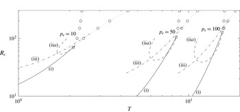
As the membrane tension increases each oscillatory neutral curve (associated with a Hopf bifurcation, figure 4) eventually intersects the line of limit points associated with loss of existence of the highly collapsed static state (dotted line in figure 4), generating a co-dimension-2 bifurcation at the intersection point and suggesting that there is a homoclinic orbit in the neighbourhood of this point (Glendinning Reference Glendinning1994). Beyond this global bifurcation point the oscillatory neutral curve terminates. Such homoclinic bifurcations are often associated with chaotic behaviour, consistent with the ‘slamming’ oscillations found in § 7.2. Similar Hopf/limit-point interactions were found by Armitstead, Bertram & Jensen (Reference Armitstead, Bertram and Jensen1996) in a lumped parameter model of self-excited oscillations in collapsible tubes.
Neutral stability curves for the three most unstable modes for fixed external pressure
 $p_{e}=10$
,
 $p_{e}=50$
and
 $p_{e}=100$
with
 $L_{2}=3$
plotting the critical Reynolds number as a function of the membrane tension. The solid lines corresponds to mode (i), the dashed line corresponds to mode (iia) and the dot-dashed line corresponds to mode (iii). The open circles connected by dotted lines represent the line of limit (saddle) points associated with a change in the number of static configurations.

To show this in more detail, figure 5 illustrates the neutral curves for branches (i), (iia) and (iii) and corresponding lines of limit points in the vicinity of the global bifurcation points for three cases
 $p_{e}=10$
,
 $p_{e}=50$
and
 $p_{e}=100$
. In all cases tested the neutral curves for branches (i) and (iia) terminate extremely close to the coalescence of the two lines of limit points, but do not seem (as far as can be determined numerically) to intersect this point.
As
 $p_{e}\rightarrow \infty$
, the value of
 $T$
at the point of intersection of the two lines of limit points (associated with a change in the number of static configurations) approaches
 $T_{c}$
while the corresponding Reynolds number
 $R\rightarrow \infty$
(figure 5), the limit point associated with the existence of the inviscid static state (appendix A). Since the neutral curves for modes (i) and (ii) always emerge very close to this intersection point, it seems that the inviscid static state is an organising centre of the dynamical system, as previously predicted by Xu et al. (Reference Xu, Billingham and Jensen2013) in a similar system but with an external pressure gradient.
In the region below and to the right of the co-dimension-2 points in the (
 $T,R$
) parameter space (figure 4) there is only one stable static configuration. However, for larger Reynolds numbers, inside the region where two static states coexist, the modes (i), (iia) all still exist and are linearly unstable. Hence, the higher modes ((iii), (iv),
 $\ldots$
) are never the primary global instability of the system. The fully nonlinear behaviour in this region is explored in § 7.2.
An alternative view of parameter space with
 $T/p_{e}$
held fixed is considered in appendix B.
5 Low-frequency oscillations as
 $p_{e}\rightarrow \infty$

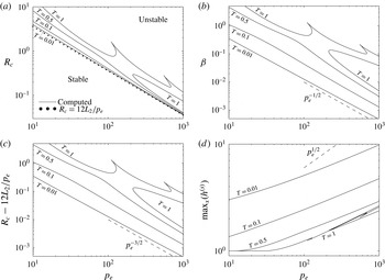
To better understand the primary oscillatory instability of the system for low membrane tensions, in figure 6(a) we illustrate the critical Reynolds number at onset as a function of external pressure
 $p_{e}$
for four fixed values of
 $T$
(showing
 $T=0.01$
,
 $T=0.1$
,
 $T=0.05$
and
 $T=1$
), with the corresponding oscillation frequency shown in figure 6(b); in this case the system is unstable above and to the right of the neutral curves. For large
 $p_{e}$
(
 $p_{e}\gtrsim 200$
) we observe that the critical Reynolds number for instability decreases proportional to
 $p_{e}^{-1}$
(figure 6
a), while the critical frequency decreases proportional to
 $p_{e}^{-1/2}$
(figure 6
b). It should be noted that the primary oscillatory branch for
 $T=1$
undergoes a resonant interaction with another mode, resulting in a mode coalescence and a cusp in the neutral curve in this parameter space, although the corresponding oscillation frequency changes smoothly. It emerges from the asymptotic analysis of appendix C that the leading-order Reynolds number takes the exceedingly simple form
 $R_{c}\approx 12L_{2}/p_{e}$
as
 $p_{e}\rightarrow \infty$
, plotted as filled circles on figure 6(a), showing excellent agreement with the numerical predictions. This serves as an estimate of the critical Reynolds number for the onset of instability as
 $T\rightarrow 0$
for fixed
 $p_{e}$
, plotted as crosses on figure 4(a) and showing good agreement with the numerical simulations. The membrane tension is sufficiently weak relative to
 $p_{e}$
, so that in the steady state we are effectively imposing boundary conditions on both
 $p_{e}$
and flux at the upstream end of the downstream segment, which produces this strong constraint on Reynolds number. In addition, to estimate the size of the first correction to the critical Reynolds number, we plot
 $R_{c}-12L_{2}/p_{e}$
as a function of
 $p_{e}$
(figure 6
c), which decreases as
 $p_{e}^{-3/2}$
.
Neutral stability curves for the primary global instability for fixed tension
 $T=0.01$
,
 $T=0.1$
,
 $T=0.5$
and
 $T=1.0$
for
 $L_{2}=3$
: (a) the critical Reynolds number for primary global instability as a function of the external pressure; (b) the corresponding mode frequency as a function of external pressure; (c) the difference between the computed critical Reynolds number and the leading-order constraint
 $R_{c}=12L_{2}/p_{e}$
as a function of external pressure; (d) the maximal expansion of the channel as a function of external pressure. The filled circles in (a) represents the asymptotic result
 $R_{c}\approx 12L_{2}/p_{e}$
. In all cases the neutral curve for
 $T=1$
is in two pieces, which may be connected for larger external pressures. The dashed line in (b) is parallel to
 $p_{e}^{-1/2}$
, the dashed line in (c) is parallel to
 $p_{e}^{-3/2}$
and the dashed line in (d) is parallel to
 $p_{e}^{1/2}$
.

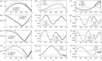
The shape of the static membrane at criticality for
 $p_{e}=1000$
and
 $T=0.01$
is shown as the solid line in figure 7(a), which is significantly bulged outwards in the centre of the domain with a narrow (slightly) collapsed region at the downstream end. To quantify this bulged state we trace the maximal membrane deflection as a function of external pressure in figure 6(d) for the four values of
 $T$
considered in figure 6. In all cases the maximal deflection increases with
 $p_{e}$
, but the scaling behaviour is more difficult to estimate as the maximal membrane deflection and the position of that maximum are both changing.
We plot the perturbation eigenfunction for
 $T=0.01$
at
 $p_{e}=1000$
in figure 7, showing the real and imaginary parts of
 $\tilde{q}$
(figure 7
b) and
 $\tilde{h}$
(figure 7
c). In this case the static wall shape has two extrema (mode-2), as has the corresponding perturbation membrane shape. This is consistent with previous studies of collapsible channel flow driven by a fixed upstream flux (Luo & Pedley Reference Luo and Pedley1996; Xu et al.
Reference Xu, Billingham and Jensen2013).
Using these observations, in appendix C we construct an asymptotic framework in the limit
 $p_{e}\rightarrow \infty$
for the leading-order profiles of the static membrane shape and the corresponding perturbation eigenfunction. Each profile is divided into two regions: a core region across the interior of the domain (region 1) and a narrow boundary layer of thickness
 $p_{e}^{-1/2}$
at the downstream end (region 2). These approximations are plotted against their numerically computed equivalents in figure 7(b,c), showing good qualitative agreement. We do not, however, use this asymptotic framework to construct the critical conditions for instability as
 $p_{e}\rightarrow \infty$
, since this requires expansion of both the static and perturbation profiles to higher orders, where the equations in each region must be solved numerically.
In a similar spirit to that described above, Stewart et al. (Reference Stewart, Waters and Jensen2009) used the present one-dimensional model with an external pressure gradient to describe the nonlinear stability of a mode-2 buckled configuration and the corresponding energy budget of oscillations. However, this study was for flow driven by a fixed upstream pressure and mechanisms of energy transfer are not comparable to the present case.
6 High-frequency oscillations as
$p_{e}\rightarrow \infty$

Close to the region of parameter space with two stable static states, the high-frequency mode labelled (iia) becomes more unstable than mode (i) and is the primary oscillatory instability of the system. The region of parameter space where this mode is dominant becomes larger as
 $p_{e}\rightarrow \infty$
(see figure 5). This mode becomes unstable through a two-branch neutral curve, as illustrated in figure 4. The asymptotic structure of modes along the lower branch of this neutral curve is described in this section.
Following the observed scaling of the neutral curves for large
 $T$
,
 $R$
and
 $p_{e}$
(figures 4 and 10) we construct an asymptotic approximation to the highly collapsed static state and the corresponding oscillatory profiles in the limit of large external pressure. We rescale
 $$\begin{eqnarray}T=p_{e}\hat{T},\quad R=p_{e}\hat{R},\quad \unicode[STIX]{x1D70E}={p_{e}}^{1/2}\hat{\unicode[STIX]{x1D70E}},\end{eqnarray}$$
where hatted quantities are assumed
 $O(1)$
. It should be noted that Xu & Jensen (Reference Xu and Jensen2015) also considered the stability of a highly constricted membrane profile using the same one-dimensional model but with an external pressure gradient. They found that the highly collapsed state is always unstable to perturbations and so they could not construct the neutral curves. Instead, they elucidated the dynamics of nonlinear ‘slamming’ motion in a slightly different dominant balance with
 $\unicode[STIX]{x1D70E}=O(1)$
and
 $L_{2}\gg 1$
, but using a three-region decomposition very similar to that considered below.
In what follows, similar to figure 10, we consider
 $\hat{T}$
and
 $L_{2}$
to be input parameters and look for the critical values of the Reynolds number
 $\hat{R}=\hat{R}_{c}$
and the corresponding critical frequency
 $\text{Im}(\hat{\unicode[STIX]{x1D70E}})=\hat{\unicode[STIX]{x1D6FD}}$
for neutral stability.
Static membrane profiles (a,d,g,j) and the real and imaginary parts of the corresponding perturbation eigenfunctions
 $\tilde{q}$
(b,e,h,k) and
 $\tilde{h}$
(c,f,i,l) at neutral stability for
 $L_{2}=3$
, showing (a–c) mode (i) for
 $T=0.01$
,
 $p_{e}=1000$
,
 $R_{c}\approx 0.03648$
; (d–f) mode (iv) for
 $T=10$
,
 $p_{e}=50$
,
 $R_{c}\approx 338.44$
; (g–i) mode (v) for
 $T=10$
,
 $p_{e}=50$
,
 $R_{c}\approx 677.65$
; (j–l) mode (iib) for
 $T=2$
,
 $p_{e}=10$
,
 $R_{c}\approx 320.09$
. The symbols on each panel denote the corresponding predictions of the asymptotic approximation in the limit of large
 $p_{e}$
for both low-frequency modes (a–c) and high-frequency modes (d–l).

Three typical static membrane profiles for modes that persist to large membrane tensions are shown in figure 7 for mode (iv) (figure 7
d), mode (v) (figure 7
g) and mode (iib) (figure 7
j). The corresponding perturbation eigenfunctions for
 $\tilde{q}$
are shown in figures 7(e,h,k) and
 $\tilde{h}$
are shown in figures 7(f,i,l). In all cases the magnitude of the real parts of
 $\tilde{q}$
are significantly greater than the imaginary part (with an exception noted below), so we assume
 $\tilde{q}$
is purely real to leading order. In a similar manner, it then follows that at neutral stability
 $\tilde{h}$
must be purely imaginary to leading order.
Following Xu & Jensen (Reference Xu and Jensen2015) we decompose the membrane profile into three asymptotic regions. We denote the asymptotic approximation to the point of maximal constriction as
 $x_{0}$
(determined in § 6.5 as part of the solution), we denote region 1 as upstream of this constriction (
 $0\leqslant x\leqslant x_{0}$
, discussed in § 6.1), region 2 as downstream of the constriction (
 $x_{0}\leqslant x\leqslant 1$
, discussed in § 6.2) and region 3 as local to this constriction (
 $x\sim x_{0}$
, discussed in § 6.3). We consider the scalings for each region in turn. In this section we denote parameters and dependent variables in the asymptotic problems with a hat, to distinguish from their equivalents in the full problem, and a numbered subscript to denote the region where that variable is defined.
We use this asymptotic approach to approximate the static solutions for a given
 $\hat{R}$
(§ 6.4) and then examine its stability by constructing the neutral oscillation frequency and corresponding point of maximal constriction (§ 6.5), the corresponding neutral stability curves (§ 6.6) and the outer approximation to the perturbation eigenfunction (§ 6.7).
6.1 Region 1
To compute an approximation to the static membrane shape in region 1 (
 $0\leqslant x\leqslant x_{0}$
, denoted with the subscript 1), we expand the static membrane profile according to
 $$\begin{eqnarray}h^{(s)}={\hat{h}}_{1}^{(s)}+O(p_{e}^{-1/2}).\end{eqnarray}$$
In region 1 the leading-order static governing equations (2.9) become
 $$\begin{eqnarray}{\hat{h}}_{1,xxx}^{(s)}=0,\quad (0\leqslant x\leqslant x_{0}),\end{eqnarray}$$
subject to boundary conditions,
 $$\begin{eqnarray}{\hat{h}}_{1}^{(s)}(0)=1,\quad {\hat{h}}_{1}^{(s)}(x_{0})=0.\end{eqnarray}$$
This system can be solved to obtain
 $$\begin{eqnarray}{\hat{h}}_{1}^{(s)}=\frac{1}{2}\overline{A}_{1}x(x-x_{0})+\frac{x_{0}-x}{x_{0}},\quad (x_{0}\leqslant x\leqslant 1),\end{eqnarray}$$
where
 $\overline{A}_{1}$
is a constant which is determined by matching into region 3.
Similarly, to construct an approximation to the perturbation eigenfunction across region 1 we expand the dependent variables according to
 $$\begin{eqnarray}\displaystyle & \displaystyle \tilde{h}=p_{e}^{-1/2}{\hat{h}}_{1}+O(p_{e}^{-1}), & \displaystyle\end{eqnarray}$$
 $$\begin{eqnarray}\displaystyle & \displaystyle \tilde{q}=\hat{q}_{1}+O(p_{e}^{-1/2}). & \displaystyle\end{eqnarray}$$
 $\hat{q}_{1}$
in the form
 $$\begin{eqnarray}\hat{\unicode[STIX]{x1D70E}}^{2}\hat{q}_{1}+\hat{T}{\hat{h}}_{1}^{(s)}\hat{q}_{1,xxxx}=0,\quad (0\leqslant x\leqslant x_{0}),\end{eqnarray}$$
subject to boundary conditions
 $$\begin{eqnarray}\displaystyle & \displaystyle \hat{q}_{1}=0,\quad \hat{q}_{1,x}=0,\quad (x=0), & \displaystyle\end{eqnarray}$$
 $$\begin{eqnarray}\displaystyle & \displaystyle \hat{q}_{1}=0,\quad \hat{q}_{1,x}=0,\quad (x=x_{0}). & \displaystyle\end{eqnarray}$$
This represents a leading-order balance between the unsteady inertial forces and the restoring force of membrane tension. It should be noted that only
 $\hat{\unicode[STIX]{x1D70E}}^{2}$
appears in the governing equations. Hence, at neutral stability (
 $\hat{\unicode[STIX]{x1D70E}}=\text{i}\hat{\unicode[STIX]{x1D6FD}}$
) the equations for real and imaginary parts of
 $\hat{q}$
decouple entirely across this region.
We solve the boundary value problem (6.5a
) using a shooting method based on the ode15s solver implemented in Matlab; simulations are initiated from
 $x=x_{0}$
, using the two specified boundary conditions (6.5c
). In addition, we adjust the values of the boundary conditions
 $\hat{q}_{1,xx}(x_{0}^{-})$
and
 $\hat{q}_{1,xxx}(x_{0}^{-})$
to isolate solutions which obey the appropriate boundary conditions at
 $x=0$
(6.5b
). However, the boundary value problem (6.5a
) is locally singular at
 $x=x_{0}$
since
 ${\hat{h}}_{1}^{(s)}(x_{0})=0$
. To initiate a numerical simulation we shoot from a small distance
 $\unicode[STIX]{x1D6FF}$
upstream of
 $x_{0}$
(
 $\unicode[STIX]{x1D6FF}\ll 1$
) towards the upstream boundary
 $(x=0)$
. We approximate the value of
 $\hat{q}_{1}$
and its derivatives at this point using a Taylor series expansion about
 $x_{0}$
. In simulations we found that a six-term Taylor series with
 $\unicode[STIX]{x1D6FF}=10^{-3}$
was sufficient to ensure convergence.
The corresponding perturbation membrane profile across region 1 is given by
 ${\hat{h}}_{1}=-\hat{q}_{1,x}/\hat{\unicode[STIX]{x1D70E}}$
. At neutral stability, assuming
 $\hat{q}_{1}$
is purely real implies that
 ${\hat{h}}_{1}$
will be purely imaginary.
6.2 Region 2
In a similar manner to region 1, across region 2 (
 $x_{0}\leqslant x\leqslant 1$
, denoted with the subscript 2), we expand the static membrane profile according to
 $$\begin{eqnarray}{\hat{h}}^{(s)}={\hat{h}}_{2}^{(s)}+O(p_{e}^{-1/2}).\end{eqnarray}$$
In region 2 the leading-order static governing equations (2.9) become
 $$\begin{eqnarray}{\hat{h}}_{2,xxx}^{(s)}=0,\quad (x_{0}\leqslant x\leqslant 1),\end{eqnarray}$$
subject to boundary conditions
 $$\begin{eqnarray}{\hat{h}}_{2}^{(s)}(x_{0})=0,\quad {\hat{h}}_{2}^{(s)}(1)=1,\quad {\hat{h}}_{2,xx}^{(s)}(1)=\hat{T}^{-1}.\end{eqnarray}$$
This system can be easily solved to obtain
 $$\begin{eqnarray}{\hat{h}}_{2}^{(s)}(x)=\frac{1}{2}\hat{T}^{-1}(x-1)(x-x_{0})+\frac{(x-x_{0})}{(1-x_{0})},\quad (x_{0}\leqslant x\leqslant 1).\end{eqnarray}$$
To construct an approximation to the perturbation eigenfunction across region 2 we expand the dependent variables according to
 $$\begin{eqnarray}\displaystyle & \displaystyle \tilde{h}=p_{e}^{-1/2}{\hat{h}}_{2}+O(p_{e}^{-1}), & \displaystyle\end{eqnarray}$$
 $$\begin{eqnarray}\displaystyle & \displaystyle \tilde{q}=\hat{q}_{2}+O(p_{e}^{-1/2}). & \displaystyle\end{eqnarray}$$
 $$\begin{eqnarray}\hat{\unicode[STIX]{x1D70E}}^{2}\hat{q}_{2}+\hat{T}h_{2}^{(s)}\hat{q}_{2,xxxx}=0,\quad (x_{0}\leqslant x\leqslant 1),\end{eqnarray}$$
subject to
 $$\begin{eqnarray}\displaystyle & \displaystyle \hat{q}_{2}=0,\quad \hat{q}_{2,x}=0,\quad (x=x_{0}), & \displaystyle\end{eqnarray}$$
 $$\begin{eqnarray}\displaystyle & \displaystyle \hat{q}_{2}=0,\quad \hat{T}\hat{q}_{2,xxx}=L_{2}\hat{\unicode[STIX]{x1D70E}}^{2}\hat{q}_{2},\quad (x=1). & \displaystyle\end{eqnarray}$$
This represents a similar balance of terms to region 1.
Again this problem is locally singular at
 $x=x_{0}$
and we employ an analogous numerical method to that described in § 6.1 to construct a solution; we shoot from a small distance
 $\unicode[STIX]{x1D6FF}$
downstream of the constriction
 $x_{0}$
using the boundary conditions (6.9b
) towards the downstream boundary at
 $x=1$
, adjusting the value of
 $\hat{q}_{2,xx}(x_{0}^{+})$
and
 $\hat{q}_{2,xxx}(x_{0}^{+})$
to identify solutions which satisfy the boundary conditions (6.9c
).
The corresponding perturbation membrane profile across region 2 is then given by
 ${\hat{h}}_{2}=-\hat{q}_{2,x}/\hat{\unicode[STIX]{x1D70E}}$
. As before, at neutral stability we assume
 $\hat{q}_{2}$
is purely real, so
 ${\hat{h}}_{2}$
must be purely imaginary.
6.3 Region 3
In region 3, close to the point of maximal constriction at
 $x=x_{0}$
, we rescale the variables according to
 $$\begin{eqnarray}x=x_{0}+p_{e}^{-1}X,\quad h^{(s)}(x)=p_{e}^{-1}{\hat{H}}_{3}^{(s)}(X)+O(p_{e}^{-3/2}).\end{eqnarray}$$
Hence, across region 3, the leading-order governing equation for the static membrane shape (2.9) becomes
 $$\begin{eqnarray}\frac{6}{5}\left(\frac{1}{{\hat{H}}_{3}^{(s)}}\right)_{X}=\hat{T}{\hat{H}}_{3}^{(s)}{\hat{H}}_{3,XXX}^{(s)},\end{eqnarray}$$
representing an inviscid balance between convective inertia and the restoring force of membrane tension. This equation is subject to continuity of slope in the far field with regions 1 and 2, in the form
 $$\begin{eqnarray}\displaystyle & \displaystyle {\hat{H}}_{3,X}^{(s)}\rightarrow \frac{1}{2}\overline{A}_{1}x_{0}-\frac{1}{x_{0}},\quad \text{as }X\rightarrow -\infty , & \displaystyle\end{eqnarray}$$
 $$\begin{eqnarray}\displaystyle & \displaystyle {\hat{H}}_{3,X}^{(s)}\rightarrow \frac{1}{2}\hat{T}^{-1}(x_{0}-1)+\frac{1}{(1-x_{0})},\quad \text{as }X\rightarrow \infty . & \displaystyle\end{eqnarray}$$
Following Xu & Jensen (Reference Xu and Jensen2015), we integrate (6.11a ) twice to form an explicit expression for the membrane slope in the form
 $$\begin{eqnarray}\hat{T}({\hat{H}}_{3,X}^{(s)})^{2}=\frac{6}{5}\left(\frac{1}{H_{0}}-\frac{1}{{\hat{H}}_{3}^{(s)}}\right),\end{eqnarray}$$
where
 ${\hat{H}}_{3}^{(s)}(0)=H_{0}$
is an unknown parameter. Following Xu & Jensen (Reference Xu and Jensen2015), we can integrate once more to obtain an implicit expression for the membrane shape across region 3,
 $$\begin{eqnarray}\sqrt{\frac{6}{5\hat{T}H_{0}^{3}}}X=\frac{1}{H_{0}}\sqrt{{\hat{H}}_{3}^{(s)}({\hat{H}}_{3}^{(s)}-H_{0})}+\log \left[H_{0}^{-1/2}\left(\sqrt{{\hat{H}}_{3}^{(s)}}+\sqrt{({\hat{H}}_{3}^{(s)}-H_{0})}\right)\right].\end{eqnarray}$$
For use below, following Xu & Jensen (Reference Xu and Jensen2015) it can also be shown that
 $$\begin{eqnarray}\int _{-\infty }^{\infty }\frac{1}{({\hat{H}}_{3}^{(s)})^{3}}\,\text{d}X=\frac{8}{3}\sqrt{\frac{5\hat{T}}{6H_{0}^{3}}}.\end{eqnarray}$$
Furthermore, to construct an approximation to the perturbation eigenfunction across region 3 we expand the dependent variables according to
 $$\begin{eqnarray}\displaystyle & \displaystyle \tilde{h}=p_{e}^{-3/2}{\hat{H}}_{3}(X)+O(p_{e}^{-2}), & \displaystyle\end{eqnarray}$$
 $$\begin{eqnarray}\displaystyle & \displaystyle \tilde{q}=p_{e}^{-1/2}\hat{Q}_{3}(X)+O(p_{e}^{-1}). & \displaystyle\end{eqnarray}$$
 $$\begin{eqnarray}\hat{Q}_{3,X}=0,\quad \hat{T}{\hat{H}}_{3,XXX}=\frac{6}{5}\left(-\frac{2\hat{Q}_{3}H_{3,X}^{(s)}}{(H_{3}^{(s)})^{3}}-\frac{{\hat{H}}_{3,X}}{(H_{3}^{(s)})^{3}}+\frac{3{\hat{H}}_{3}{\hat{H}}_{3,X}^{(s)}}{(H_{3}^{(s)})^{4}}\right),\end{eqnarray}$$
subject to appropriate matching conditions into regions 1 and 2. However, noting that these equations are symmetric in
 $X$
we find below that we do not need to solve the perturbation equations in this region explicitly to construct the outer approximation to the eigenfunctions.
6.4 The composite static solution
Matching the expression for
 ${\hat{H}}_{3,X}^{(s)}$
as
 $X\rightarrow -\infty$
into region 1 we obtain the constant
 $\overline{A}_{1}$
in the form
 $$\begin{eqnarray}\overline{A}_{1}=\hat{T}^{-1}\frac{1-x_{0}}{x_{0}}-\frac{2(2x_{0}-1)}{x_{0}^{2}(1-x_{0})},\end{eqnarray}$$
while matching the expression for
 ${\hat{H}}_{3,X}^{(s)}$
as
 $X\rightarrow \infty$
into region 2 we obtain a constraint for
 $H_{0}$
as a function of
 $x_{0}$
,
 $$\begin{eqnarray}\frac{6}{5}\left(\frac{1}{H_{0}}\right)=\frac{1}{2}\frac{(x_{0}-1)}{\hat{T}}+\frac{1}{1-x_{0}}.\end{eqnarray}$$
This fully specifies the leading-order static solution across all three regions for a given
 $x_{0}$
. Using the value of
 $x_{0}$
calculated in § 6.5 and the critical value of Reynolds number
 $\hat{R}$
calculated in § 6.6, we thus plot the approximation to the membrane shape across the three regions in figure 7 for three examples (figure 7
d,g,j), showing excellent qualitative agreement with full numerical simulations in the first two cases; a discussion of the discrepancy for mode (2,1) is given in § 6.7.
6.5 The oscillation frequency and point of maximal constriction
Since we are only concerned with neutrally stable oscillations, we express
 $\hat{\unicode[STIX]{x1D70E}}^{2}=-\hat{\unicode[STIX]{x1D6FD}}^{2}$
and conduct all calculations in terms of
 $\hat{\unicode[STIX]{x1D6FD}}$
. Given that
 $\hat{\unicode[STIX]{x1D6FD}}^{2}$
is purely real at neutral stability, the form of the governing equations (6.5a
), (6.9a
) mean that the real and imaginary parts of
 $\hat{q}$
can be considered independently at this order.
Across region 3 we observe that the membrane profile is symmetric to leading order, so that the limiting slopes from regions 1 and 2 are equal and opposite,
 $$\begin{eqnarray}\lim _{x\rightarrow x_{0}^{+}}{\hat{h}}_{2,x}=-\lim _{x\rightarrow x_{0}^{-}}{\hat{h}}_{1,x}.\end{eqnarray}$$
Since the solution to the linearised system (2.11) can be normalised arbitrarily, we set
 $\hat{q}_{xx}(x_{0}^{+})=1=-\hat{q}_{xx}(x_{0}^{-})$
without loss of generality (since
 $\hat{q}_{xx}$
is proportional to
 ${\hat{h}}_{x}$
through (2.11a
)). For a given value of
 $x_{0}$
we compute the corresponding values of
 $\hat{\unicode[STIX]{x1D6FD}}$
and
 $\hat{q}_{xxx}(x_{0}^{-})$
(
 $\hat{q}_{xxx}(x_{0}^{+})$
) such that the solution satisfies the upstream (downstream) boundary conditions, from which we trace out curves in the parameter space spanned by
 $x_{0}$
and
 $\hat{\unicode[STIX]{x1D6FD}}$
; each curve represents a different number of extrema in the profile of
 $\tilde{h}$
denoting
 $m$
(
 $n$
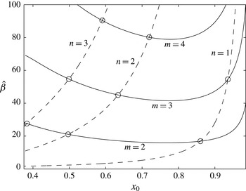
) turning points upstream (downstream) of the point of maximal constriction. In figure 8, typical curves for
 $m=2$
,
 $m=3$
and
 $m=4$
are shown as solid lines while curves for
 $n=1$
,
 $n=2$
and
 $n=3$
are shown as dashed lines, computed for
 $\hat{T}=0.2$
and
 $L_{2}=3$
. Numerical tests indicate there is no curve for
 $m=1$
. Points of intersection between upstream (solid) and downstream (dashed) curves in figure 8 represent global roots of the full system. These global crossing points correspond to distinct modes with a particular
 $(m,n)$
; the critical values of
 $x_{0}$
and
 $\hat{\unicode[STIX]{x1D6FD}}$
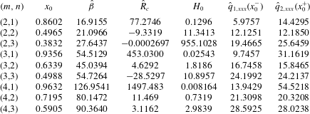
for the first nine modes are listed in table 1, along with the corresponding shooting parameters.
Parameter space spanned by the position of the membrane minimum
 $x_{0}$
against the corresponding oscillation frequency
 $\hat{\unicode[STIX]{x1D6FD}}$
for
 $\hat{T}=0.2$
and
 $L_{2}=3$
. Solid (dashed) lines represent solutions which satisfy the upstream (downstream) boundary conditions. Crossing points represent global roots of the asymptotic system.

Shooting parameters for the nine eigenmodes shown on figure 8 computed for
 $\hat{T}=0.2$
and
 $L_{2}=3$
.

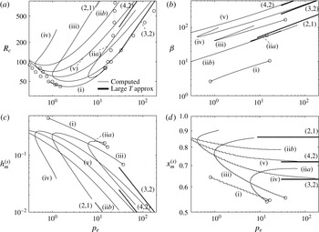
The asymptotic prediction of the critical frequencies for modes (3,2), (4,2) and (2,1) are plotted against the full numerical solutions as filled circles in figures 4(c) and 10(b). We find excellent agreement with the computed frequencies, with the mode (2,1) corresponding to neutral curve (iib), the mode (3,2) corresponding to neutral curve (iv) and the mode (4,2) corresponding to the neutral curve (v). In addition, the corresponding asymptotic prediction of the maximal constriction (
 $p_{e}^{-1}H_{0}$
) and the point of greatest constriction (
 $x_{0}$
) are shown in figures 10(c) and 10(d), respectively, against the full numerical computations. In both cases the curves (3,2) and (4,2) show excellent agreement with the numerical computations for neutral curves (iv) and (v). The curve (2,1) shows the correct trend as neutral curve (iib), but is slightly separated. The origin of this discrepancy is explored in § 6.7.
6.6 The critical Reynolds number
Applying the scalings for regions 1 to 3 into the energy budget for static solutions (2.17), we obtain the leading-order relationship
 $$\begin{eqnarray}\hat{T}({\hat{h}}_{2,xx}^{(s)}(1)-{\hat{h}}_{1,xx}^{(s)}(0))=\frac{12}{\hat{R}}\int _{-\infty }^{\infty }\frac{1}{({\hat{H}}_{3}^{(s)})^{3}}\,\text{d}X,\end{eqnarray}$$
so the rate of working of pressure forces along the compliant segment of the channel is balanced by the viscous losses close to the point of greatest channel constriction. Substituting the analytical expressions for
 $h_{1}^{(s)}$
,
 $h_{2}^{(s)}$
constructed above (6.3d
) and (6.7e
) and the integral (6.14), we obtain the constraint
 $$\begin{eqnarray}\frac{1}{\hat{T}x_{0}}+\frac{2(2x_{0}-1)}{x_{0}^{2}(1-x_{0})}=\frac{32}{\hat{R}}\left(\frac{5\hat{T}}{6H_{0}^{3}}\right)^{1/2}.\end{eqnarray}$$
For a given
 $x_{0}$
and
 $\hat{\unicode[STIX]{x1D6FD}}$
computed using the method outlined above, the corresponding critical Reynolds number can be computed using (6.21). These predictions are listed in table 1 and the corresponding predictions of the neutral curves are shown in figures 4(a) and 10(a) for modes (2,1), (3,2) and (4,2). As
 $p_{e}\rightarrow \infty$
the neutral curves each show the correct trend and approach the numerically computed curves, although the values of
 $p_{e}$
considered here are not sufficiently large to demonstrate a strong overlap (as discussed above, we found that an unfeasible number of grid points were needed to resolve the static profile for larger values of
 $p_{e}$
). There is a more marked discrepancy for the mode labelled (2,1), which is discussed below. For some of the roots identified in table 1 the corresponding critical Reynolds number is negative, indicating an unphysical solution for those
 $(m,n)$
and that choice of parameters
 $\hat{T}$
and
 $L_{2}$
.
6.7 Outer approximation to the eigenfunctions
Given the approximate eigenfunction profiles constructed across regions 1 and 2 in § 6.5, the outer asymptotic eigenfunctions for three particular examples are shown in figure 7(d–l) for
 $\hat{T}=0.2$
and
 $L_{2}=3$
. Note that the outer asymptotic eigenfunction has been normalised in the same way as the numerically computed eigenfunctions for ease of comparison. In particular, we consider mode (3,2) in figure 7(e,f), where
 $R_{c}\approx 338.44$
(
 $p_{e}\hat{R}_{c}\approx 216.30$
), mode (4,2) in figure 7(h,i), where
 $R_{c}\approx 677.65$
(
 $p_{e}\hat{R}_{c}\approx 532.15$
) and mode (2,1) in figure 7(k,l), where
 $R_{c}\approx 320.09$
(
 $p_{e}\hat{R}_{c}\approx 605.69$
). For modes (3,2) and (4,2) we observe excellent qualitative agreement between the numerically computed eigenfunctions and the outer asymptotic approximation. However, for mode (2,1) the agreement is weaker, exacerbated by the large discrepancy in the estimate of the point of maximal constriction (figure 10
d). A possible explanation for this discrepancy lies in the shape of the eigenfunction downstream of the constriction. In this region, unlike for the other examples shown, the real and imaginary parts of
 $\tilde{q}$
are comparable (figure 10
d,ii), so our assumption that
 $\tilde{q}$
is purely real is not appropriate. Furthermore, the slopes of the perturbation membrane shape upstream and downstream of the constriction are clearly not equal and opposite (figure 10
d,iii), in contradiction of our leading-order asymptotic theory. To improve the prediction of this mode would require coupling of the real and imaginary parts of the eigenfunction at leading order, which is not considered here.
7 Fully nonlinear simulations
In this section we use fully nonlinear simulations of the PDEs (2.8) to examine the nonlinear development of the primary global instability (§ 7.1), the development of nonlinear ‘slamming’ oscillations for large Reynolds numbers (§ 7.2) and finally the corresponding nonlinear energy budget of fully developed oscillations (§ 7.3).
7.1 Primary global instability
We use nonlinear simulations of (2.8) to trace the behaviour along two lines in parameter space with
 $p_{e}=10$
and
 $L_{2}=3$
, the first for
 $T=2$
, where the collapsed basic state exists for all
 $R$
(§ 7.1), and the second for
 $T=2.7$
, where the collapsed basic state (§ 7.2) does not exist for sufficiently small
 $R$
.
Fully nonlinear simulations for
 $p_{e}=10$
and
 $L_{2}=3$
: (a) bifurcation diagram of
 $h_{m}$
against
 $R$
for
 $T=2$
, tracing the maximum (filled circles) and minimum (crosses) of
 $h_{m}(t)$
over a period of oscillation; time traces of the membrane minimum
 $h_{m}$
for (b)
 $T=2$
,
 $R=61$
, where the response is asymptotically stable; (c)
 $T=2$
,
 $R=65$
, where the oscillatory response has undergone a period doubling bifurcation; (d)
 $T=2.7$
,
 $R=120$
where the oscillation again saturates the almost uniform static state; (e)
 $T=2.7$
,
 $R=130$
where the oscillation saturates the almost uniform static state; (f)
 $T=2.7$
,
 $R=170$
where the oscillation saturates to a large-amplitude limit cycle with ‘slamming’. The triangles in (a) illustrate the mean position of the membrane minimum over a period, while the thick black lines indicate the range of values for the maximum and minimum of
 $h_{m}$
for the chaotic oscillations.

We examine the primary global instability close to the neutral point for
 $T=2$
,
 $p_{e}=10$
for
 $L_{2}=3$
, where the collapsed basic state becomes unstable to an oscillatory instability (via a Hopf bifurcation) as the Reynolds number increases through the threshold
 $R=R_{c}\approx 62.24$
. In simulations we employ an initial condition
 $$\begin{eqnarray}h(x,0)=h^{(s)}(x)+A\text{Re}(\tilde{h}(x;\unicode[STIX]{x1D70E})),\quad q(x,0)=1+A\text{Re}(\tilde{q}(x;\unicode[STIX]{x1D70E})),\end{eqnarray}$$
where
 $A=0.01$
in simulations. In figure 9(a) we numerically trace a bifurcation diagram by plotting the minimal and maximal values of
 $h_{m}$
over a period of fully developed oscillation as a function of
 $R$
. Figure 9(a) indicates that the Hopf bifurcation is supercritical. For
 $R<R_{c}$
the static membrane is asymptotically stable (figure 9
b). However, as the Reynolds number increases the oscillation undergoes a period doubling bifurcation (evident for
 $R=65$
, see figure 9
c) and eventually becomes chaotic (evident for
 $R=66$
,
 $R=67$
, where the thick black lines indicate the range of values for the maximum and minimum of
 $h_{m}$
). Also shown on figure 9(a) is the mean position of the membrane minimum over a period of oscillation, denoted
 $\overline{h_{m}}$
(illustrated as open triangles connected by a dotted line) compared to the minimal value of the corresponding static membrane (solid line). We observe that the mean minimal channel width is increased slightly compared to the static solution, which has consequences for the energy transfer mechanism sustaining the oscillation (see § 7.3).
7.2 Fully nonlinear ‘slamming’ oscillations
We examine the secondary global instabilities by considering the fully nonlinear behaviour close to a region where the collapsed basic state does not exist, in particular for
 $T=2.7$
,
 $p_{e}=10$
for
 $L_{2}=3$
. For
 $R>R_{b}\approx 127.8$
we use the initial condition (7.1a,b
). For lower Reynolds numbers (
 $R<R_{b}$
) the highly collapsed steady state does not exist. Starting close to the almost uniform static state the system is asymptotically stable (not shown). Hence, we choose to start the simulations close to the highly collapsed static state computed for some
 $R>R_{b}$
(here we choose an initial state generated for
 $R=130$
). For
 $R=120$
the system oscillates initially but eventually saturates towards the almost uniform static state, as in figure 9(d). For
 $R>R_{b}$
the perturbation growth becomes increasingly oscillatory and irregular as
 $R$
increases, where there are two possible attractors for long times. For some parameter choices inside the dark shaded region in figure 4(b) (where there are two concurrent static states) the system oscillates initially but eventually saturates to the almost uniform static profile, as shown in figure 9(e) for
 $R=130$
; for other parameter choices the system exhibits a fully developed oscillatory (typically chaotic) limit cycle, where periodically the membrane is drawn very close to the rigid wall before recovering (see example for
 $R=170$
in figure 9
f). These so-called ‘slamming’ oscillations have been observed previously (Stewart Reference Stewart2010; Stewart et al.
Reference Stewart, Heil, Waters and Jensen2010; Xu et al.
Reference Xu, Billingham and Jensen2013) and can be deconstructed using matched asymptotic expansions (Xu & Jensen Reference Xu and Jensen2015). As the Reynolds number increases the ‘slamming’ oscillation eventually becomes dominant. It is interesting to note that in this case linear instability to oscillations does not necessarily result in an unsteady outcome for long times, similar to predictions of three-dimensional flow in a collapsible tube by Heil & Boyle (Reference Heil and Boyle2010).
7.3 Energy budget of the primary global instability
Finally, we examine the energy budget of the self-excited oscillations to elucidate the driving mechanism. We define the time average of a quantity
 $f(x,t)$
over a period of oscillation
 $T_{f}$
according to
 $$\begin{eqnarray}\overline{f}(x)=\frac{1}{T_{f}}\int _{0}^{T_{f}}f(x,t)\,\text{d}t.\end{eqnarray}$$
In particular we consider a parameter sweep along the line
 $T=2$
for
 $p_{e}=10$
,
 $L_{2}=3$
where the critical Reynolds number
 $R_{c}\approx 62.24$
corresponds to the mode labelled (i) in figure 4. The terms in the full energy budget (2.13a
) are computed for various
 $R>R_{c}$
from the nonlinear simulations and their time average calculated over a period of fully saturated oscillation and listed in table 2. Also listed in the table are the terms in the energy budget for the corresponding static state, denoted with the superscript
 $(s)$
.
We compute the energy budget of the oscillation by subtracting the energy corresponding to the static state, computing the excess work done by upstream pressure forces over a period (
 $\overline{{\mathcal{P}}^{(e)}}=\overline{{\mathcal{P}}}-{\mathcal{P}}^{(s)}$
) and the excess rate of working of viscous dissipation (
 $\overline{{\mathcal{D}}^{(e)}}=\overline{{\mathcal{D}}_{S}}-{\mathcal{D}}^{(s)}$
). It emerges that over a period the dominant energy balance is between these excess energies,
 $\overline{{\mathcal{P}}^{(e)}}$
and
 $\overline{{\mathcal{D}}^{(e)}}$
, while the net kinetic energy flux extracted from the mean flow (
 $\overline{{\mathcal{F}}}$
) and the kinetic energy flux induced by the flow profile assumption (
 $\overline{{\mathcal{D}}_{A}}$
) are both very small in comparison (see table 2). This is in direct agreement with the observations of Liu et al. (Reference Liu, Luo and Cai2012) in a flow-driven collapsible channel system.
As discussed in § 2.4, we further decompose
 $\overline{{\mathcal{D}}_{S}}$
using the global linear stability eigensolver, where (2.19) implies
 $$\begin{eqnarray}\overline{{\mathcal{D}}^{(e)}}\approx \unicode[STIX]{x1D703}^{2}(\overline{\tilde{{\mathcal{D}}}_{S}}+\overline{\breve{{\mathcal{D}}}_{S}}),\end{eqnarray}$$
for
 $\unicode[STIX]{x1D703}\ll 1$
. In the fully nonlinear computations we find
 $\overline{{\mathcal{D}}^{(e)}}<0$
for all cases tested (see table 2). However, computing
 $\overline{\hat{{\mathcal{D}}}_{S}}$
for these parameter values at criticality (
 $T=2$
,
 $p_{e}=10$
,
 $L_{2}=3$
,
 $R_{c}\approx 62.24$
) using the perturbation eigenfunctions
 $\tilde{h}$
and
 $\tilde{q}$
we find that
 $\overline{\hat{{\mathcal{D}}}_{S}}>0$
. Hence, dissipative forces in the perturbation are consuming energy, so the perturbation dissipation in the mean flow,
 $\overline{\breve{{\mathcal{D}}}_{S}}$
, must be negative. Hence, the presence of the oscillation reduces the overall dissipation of the mean flow (through the work of nonlinear Reynolds stresses) and this excess energy drives the oscillation. However, this reduction of the dissipation is not achieved by modifying the mean flow along the channel as we need
 $\overline{q}(1,t)=1$
(i.e.
 $\overline{\check{q}}=0$
) to satisfy conservation of mass over a period of neutrally stable oscillation. Instead this reduction in dissipation is achieved by decreasing the mean maximal constriction of the channel over a period of neutrally stable oscillation, so
 $\overline{h_{m}}>h_{m}^{(s)}$
. This is illustrated in the fully nonlinear bifurcation diagram in figure 9(a) and the computed values of
 $\overline{h_{m}}$
and
 $h_{m}^{(s)}$
are listed in table 2.
A similar mechanism of energy transfer is operating for the mode labelled (iia), corresponding to the most unstable member of the family of high-frequency oscillations explored in § 6.



8 Discussion
In this paper we have considered the stability of laminar high-Reynolds-number flow through a planar channel, where a section of one wall has been replaced by a tensioned membrane; this tension is assumed sufficiently large to dominate the influence of bending stiffness and other elastic restoring forces. The model also neglects other wall parameters such as the wall inertia and viscous damping, although the role of these parameters will be considered in future work. To reduce the computational complexity, we construct a spatially one-dimensional model derived using a von Karman–Pohlhausen approximation, in a similar manner to earlier studies of flow through a flexible-walled channel (Stewart et al. Reference Stewart, Waters and Jensen2009; Xu et al. Reference Xu, Billingham and Jensen2013, Reference Xu, Billingham and Jensen2014; Xu & Jensen Reference Xu and Jensen2015). This model has a number of limitations, most its notably failure to capture the influence of dissipation in narrow boundary layers that will arise at large Reynolds numbers and frequencies. In addition, this model fails to capture energy losses associated with flow separation (discussed below) and the generation of so-called vorticity waves in the downstream rigid segment (a striking feature of computational simulations driven by fixed upstream flux, Luo & Pedley (Reference Luo and Pedley1996)). However, this model has previously been demonstrated to give good qualitative agreement with full numerical simulations at modest Reynolds numbers, successfully predicting several families of self-excited oscillations also found in the full two-dimensional system including ‘sloshing’ oscillations (Jensen & Heil Reference Jensen and Heil2003; Stewart et al. Reference Stewart, Waters and Jensen2009), ‘sawtooth’ oscillations (Xu et al. Reference Xu, Billingham and Jensen2014) and nonlinear ‘slamming’ oscillations (Stewart et al. Reference Stewart, Heil, Waters and Jensen2010). The model also provides a method for examining large sections of the parameter space with relatively low computational cost.
Energy losses associated with flow separation were a key feature of earlier one-dimensional models of oscillations in collapsible tubes (e.g. Cancelli & Pedley Reference Cancelli and Pedley1985; Jensen Reference Jensen1990), necessary for the system to exhibit instability in the absence of other sources of dissipation. In the present model, the additional energy losses due to flow separation might be expected to increase the critical Reynolds number required for instability of our global modes. This hypothesis is corroborated by preliminary simulations of our linear stability eigensolver where the convective inertia term in (2.8c
) is multiplied by a constant
 $\unicode[STIX]{x1D712}<1$
in the region downstream of maximal constriction, in a similar manner to previous one-dimensional models (e.g. Cancelli & Pedley Reference Cancelli and Pedley1985; Jensen Reference Jensen1990). However, such a crude modification fails to accurately account for the recirculation region in the flow downstream of the point of separation (see Luo & Pedley Reference Luo and Pedley2000) and its influence on the dissipative losses, neither of which can be rationally captured within our flow profile assumption. A more complete examination of the influence of flow separation on our predicted modes of oscillation is therefore deferred to future work.
In particular, we consider a constant external pressure applied to the flexible membrane, in contrast to previous studies using this one-dimensional model which all imposed an external pressure gradient which is difficult to realise experimentally. The flow is driven by a fixed upstream flux, and we demonstrate that the system admits at least one non-uniform static state at all points across the parameter space. For sufficiently large Reynolds numbers, across a range of membrane tensions the system exhibits three possible static solutions, two of which are stable to (static) perturbations (figure 2). This prediction of multiple coexisting steady states is consistent with previous one-dimensional models of collapsible tube flow (Reyn Reference Reyn1987; Siviglia & Toffolon Reference Siviglia and Toffolon2014) and full numerical computations of flow through flexible-walled channels (Luo & Pedley Reference Luo and Pedley2000) and tubes (Heil & Boyle Reference Heil and Boyle2010).
The static predictions of figure 2(a) can be represented in an alternative manner, plotting the flow rate along the channel as a function of the applied driving pressure, while holding the difference between the upstream and external pressures constant. Similar to previous studies (e.g. Jensen Reference Jensen1998; Luo & Pedley Reference Luo and Pedley2000; Stewart Reference Stewart2010), the flow rate eventually becomes limited by the constriction and does not continue to increase with increasing driving pressure. Such ‘flow limitation’ or ‘choking’ can occur physiologically when forced expiration from the lungs causes airways to collapse, restricting the flow of air (Gavriely & Grotberg Reference Gavriely and Grotberg1988). In previous one-dimensional models, such choking behaviour was associated with a transition through the critical state (Kececioglu et al. Reference Kececioglu, Mcclurken, Kamm and Shapiro1981; Cancelli & Pedley Reference Cancelli and Pedley1985; Elad, Kamm & Shapiro Reference Elad, Kamm and Shapiro1987) i.e. the flow speed approaching the local wave speed. A more recent study by Siviglia & Toffolon (Reference Siviglia and Toffolon2013) showed how these transcritical conditions could be induced by discontinuous mechanical properties of the flexible vessel, physiologically mimicking a stent or region of tissue whose properties have been altered by surgery. However, given the dispersive nature of the current model it is not clear if a similar transition occurs in our predictions.
For low Reynolds numbers the system is asymptotically stable. However, as the Reynolds number increases (holding other parameters fixed) the static configuration becomes unstable to self-excited oscillations via a supercritical Hopf bifurcation. The non-uniform state is unstable to two infinite families of oscillatory normal modes, all with distinct neutral curves. Some of these neutral curves trace out two-branch tongues beyond a critical membrane tension, similar to those found by Luo et al. (Reference Luo, Cai, Li and Pedley2008), while others persist for all tensions (figures 4 and 10). Testing of these new predictions against full two-dimensional computations is an interesting avenue of future work.
For sufficiently low membrane tensions, the primary global instability of the system is to a low-frequency mode where the frequency of oscillation decreases as
 $p_{e}$
increases; the corresponding eigenfunction for the perturbation membrane shape has two extrema for low tensions (mode-2) (figure 7
c) but changes form along the neutral curve as the tension increases (figure 3
b). As
 $p_{e}\rightarrow \infty$
the mode-2 static membrane shape arises from an outwardly bulged region in the centre of the domain with a narrow constriction at the downstream end (figure 7
a). The corresponding neutral stability curves continue as
 $T\rightarrow 0$
, and the corresponding critical Reynolds number at onset takes the simple form
 $R_{c}=12L_{2}/p_{e}$
as
 $p_{e}\rightarrow \infty$
(figure 6
a). It is interesting to note that the parameter regime where this instability is predicted (low Reynolds number, low-frequency oscillations) is exactly that where the present one-dimensional model is expected to be an accurate reflection of the full two-dimensional system.
For larger membrane tensions, we identified an alternative asymptotic regime where the frequency of oscillation increases with increasing external pressure (figure 4
c). Most of these high-frequency modes exhibit a two-branch neutral curve, unstable beyond a critical value of the tension (figure 4
a). For modes along the lower branch of these neutral curves, either side of the point of maximal constriction there is a leading-order balance between the unsteady inertia and the restoring force of membrane tension. This leading-order balance (along with the observation that the oscillation frequency increases with the square root of the membrane tension), is identical to that observed for ‘sloshing’ instabilities driven by fixed upstream pressure (Jensen & Heil Reference Jensen and Heil2003; Stewart et al.
Reference Stewart, Waters and Jensen2009). However, in the present case the dominant source of viscous dissipation arises around the point of greatest constriction of the static membrane, whereas for ‘sloshing’ modes predicted in using an analogue of our 1D model the dominant dissipation arises over entire channel (Stewart et al.
Reference Stewart, Waters and Jensen2009). (Of course, in the full 2D and 3D representations of ‘sloshing’ the dominant dissipation is confined to narrow Stokes layers on the channel walls (Jensen & Heil Reference Jensen and Heil2003; Whittaker et al.
Reference Whittaker, Heil, Jensen and Waters2010).) In addition, in ‘sloshing’ the mean flow rate along the channel is increased by the oscillation, whereas here the mean flow must remain constant (due to the choice of upstream boundary condition) and instead the channel walls are driven apart over a period, releasing energy which drives the oscillation. Hence, although the leading-order balance of terms is broadly similar, the fundamental mechanism of instability elucidated herein is very different to ‘sloshing’. The asymptotic structure divides the perturbation membrane profile into two distinct segments and leads to a new naming convention: mode
 $(m,n)$
has
 $m$
extrema upstream of the point of greatest constriction and
 $n$
extrema downstream. Predictions of modes (3,2) and (4,2) (and to a lesser extent mode (2,1)) all agree well with the corresponding numerical computations (figures 4 and 10) as
 $p_{e}$
becomes large.
In regions of the parameter space where the system exhibits two stable static states (e.g. shaded region in figure 4 b), nonlinear simulations of the governing equations about the highly collapsed static state exhibit one of two possible behaviours, depending on the choice of initial perturbation: in some cases the unsteady oscillation is eventually suppressed and the system asymptotes towards the almost uniform static state (figure 9 d), while in others the system enters a large-amplitude chaotic ‘slamming’ limit cycle (figure 9 e), as has been observed previously in a similar system driven by fixed upstream flux (Xu et al. Reference Xu, Billingham and Jensen2013, Reference Xu, Billingham and Jensen2014; Xu & Jensen Reference Xu and Jensen2015). This chaotic response is consistent with the presence of homoclinic (global) bifurcation points nearby in the parameter space, which result from the intersection between the oscillatory neutral curves (associated with a supercritical Hopf bifurcation) and the line of limit points associated with loss of existence of the highly collapsed static state (figure 5).
The system considered herein, flow-driven oscillations about a highly collapsed static configuration, is reminiscent of instabilities generated by fluid–structure interaction in the vocal folds in the human larynx (see Mittal, Erath & Plesniak Reference Mittal, Erath and Plesniak2013, for a recent review), with the external pressure playing the role of the tissue pressure in the folds. A qualitative comparison between our predictions and experiments on a mechanical replica of the human vocal tract is an interesting direction for future work. The model presented herein also has potential bio-mechanical application to snoring and sleep apnea (e.g. Gavriely & Jensen Reference Gavriely and Jensen1993).
Acknowledgements
Helpful discussions with Professor O. Jensen (University of Manchester), Professor X. Luo and Miss D. Wang (both University of Glasgow) are very gratefully acknowledged. Funding from EPSRC grant no. EP/N014642/1 is gratefully acknowledged. The data for the simulations presented in this paper can be accessed online (http://dx.doi.org/10.5525/gla.researchdata.412).
Appendix A. Inviscid static solutions for fixed upstream flux
Xu et al. (Reference Xu, Billingham and Jensen2013) found that their system (almost identical to (2.9) but with an imposed external pressure gradient to maintain a uniform basic state) admitted a countably infinite number of static, inviscid eigenmodes for particular values of the dimensionless membrane tension,
 $$\begin{eqnarray}T_{n}=\frac{6}{5n^{2}\unicode[STIX]{x03C0}^{2}},\quad n=0,1,2,\ldots .\end{eqnarray}$$
These critical values of the tension serve as organising centres for the dynamical system, as elucidated by Xu et al. (Reference Xu, Billingham and Jensen2013).
In a similar spirit, we examine the inviscid limit of the static governing equations (2.9) for fixed external pressure, where the equations take the form
 $$\begin{eqnarray}\frac{6}{5}\left(\frac{1}{h^{(s)}}\right)_{x}=Th^{(s)}h_{xxx}^{(s)},\quad (0\leqslant x\leqslant 1),\end{eqnarray}$$
subject to three boundary conditions
 $$\begin{eqnarray}\displaystyle & \displaystyle h^{(s)}=1,\quad (x=0), & \displaystyle\end{eqnarray}$$
 $$\begin{eqnarray}\displaystyle & \displaystyle h^{(s)}=1,\quad Th_{xx}^{(s)}=p_{e},\quad (x=1), & \displaystyle\end{eqnarray}$$
independent of the downstream length of the channel,
 $L_{2}$
. These static inviscid governing equations (A 2) can be integrated exactly to obtain a second-order ODE
 $$\begin{eqnarray}\frac{3}{5}\left(\frac{1}{(h^{(s)})^{2}}-1\right)=Th_{xx}^{(s)}-p_{e},\quad (0\leqslant x\leqslant 1),\end{eqnarray}$$
subject to
 $h^{(s)}(0)=h^{(s)}(1)=1$
. This equation can be integrated once more with respect to
 $x$
, but it was not possible (to the best of our knowledge) to find a closed form solution for
 $h^{(s)}(x)$
. However, (A 3) can be easily solved numerically and the properties of
 $h^{(s)}$
can be traced as a function of the model parameters. It emerges that for a given
 $p_{e}$
there are two branches of inviscid static solutions for
 $T>T_{c}$
, beyond a limit point at
 $T=T_{c}$
, as shown in figure 2: a stable upper branch and an unstable lower branch. For
 $p_{e}=10$
, the critical value of
 $T$
above which these static inviscid solutions exist is
 $T_{c}\approx 2.426$
, much greater than the largest admissible value of membrane tension found by Xu et al. (Reference Xu, Billingham and Jensen2013) listed in (A 1), representing a significant difference between application of a fixed external pressure and an external pressure gradient.
Appendix B. Numerical results for
$\hat{T}$
constant

We further illustrate the parameter space of neutrally stable oscillations in an alternative manner, holding both the downstream channel length and ratio of membrane tension to external pressure fixed (
 $\hat{T}=T/p_{e}=\text{const}.$
, where
 $\hat{T}=T_{0}/(\unicode[STIX]{x1D70C}a(P_{e}-P_{0}))$
in terms of dimensional variables). This choice of scaling is consistent with the asymptotic structure identified in § 6. For example, setting
 $\hat{T}=0.2$
and
 $L_{2}=3$
the corresponding neutral curves for the six most unstable modes traced in figure 4, plotting the critical value of the Reynolds number as a function of the external pressure, are shown in figure 10(a), the corresponding oscillation frequency (figure 10
b), the maximal constriction of the collapsed static channel (
 $h_{m}^{(s)}$
, figure 10
c) and the corresponding
 $x$
-position of the that maximal constriction (
 $x_{m}^{(s)}$
, figure 10
d). The latter exhibits a step-wise structure as the membrane shape is solved on a uniform grid, so the location of the membrane minimum changes discretely. In this case the lower branch of the neutral curves become parallel in the limit as
 $p_{e}\rightarrow \infty$
and again terminate at a co-dimension-2 (global) bifurcation. As in figure 4, the neutral curves that do not terminate in an open circle continue to larger values of
 $p_{e}$
than those considered here.
Neutrally stable oscillations for
 $\hat{T}=T/p_{e}=0.2$
and
 $L_{2}=3$
as a function of the external pressure
 $p_{e}$
: (a) the critical value of the Reynolds number of instability for the five most unstable modes labelled (i–v); (b) corresponding frequency of the neutrally stable modes; (c) minimal value of the constriction of the static state
 $h_{m}^{(s)}$
; (d) the location of the minimal value of the static constriction,
 $x_{m}^{(s)}$
. Also shown are the corresponding asymptotic predictions for large
 $p_{e}$
for the three modes with lower branch that persists for
 $p_{e}\rightarrow \infty$
.

Appendix C. Low-frequency oscillations for
$p_{e}\rightarrow \infty$

In this appendix we outline the asymptotic structure of the low-frequency instabilities in the limit
 $p_{e}\rightarrow \infty$
, considering the leading-order static configuration and the corresponding leading-order perturbation eigenfunction. However, we do not calculate the critical conditions for the onset of instability, which follow from higher orders. We assume the flow can be decomposed into two asymptotic regions, a core region of
 $O(1)$
width across the interior of the domain, where the static profile of the membrane is highly bulged outwards, denoted as region 1 (§ C.1), and a narrow boundary layer at the downstream end of width
 $p_{e}^{-1/2}\ll 1$
, denoted as region 2 (§ C.2). We now consider each region in turn. In this appendix we denote the parameters and independent variables in the asymptotic problems with a breve to distinguish from their equivalents in the full problem, and a numbered subscript to denote the region where the variable is defined.
We assume that the critical Reynolds number can be expanded in powers of
 $p_{e}^{-1/2}$
in the form
 $$\begin{eqnarray}R_{c}={p_{e}}^{-1}(\breve{R}_{c}+p_{e}^{-1/2}\breve{R}_{p}+\cdots ),\end{eqnarray}$$
where breved variables are
 $O(1)$
. Furthermore, we rescale the membrane tension parameter in the form
 $T=p_{e}^{-1/2}\breve{T}$
, where
 $\breve{T}=O(1)$
, so this family of self-excited oscillations exists for low membrane tensions.
We consider neutrally stable oscillations and restrict attention to the case
 $\unicode[STIX]{x1D70E}=\text{i}\unicode[STIX]{x1D6FD}$
(the case
 $\unicode[STIX]{x1D70E}=-\text{i}\unicode[STIX]{x1D6FD}$
follows in an identical manner). We expand this critical frequency in the form
 $$\begin{eqnarray}\unicode[STIX]{x1D6FD}=p_{e}^{-1/2}\breve{\unicode[STIX]{x1D6FD}}+O(p_{e}^{-1}).\end{eqnarray}$$
In the analysis below we will assume that at leading order the perturbation eigenfunction
 $\tilde{h}$
is purely real and
 $\tilde{q}$
is purely imaginary, consistent with the numerical examples in figure 7(b,c).
C.1 Region 1
Across region 1 (
 $0\leqslant x\leqslant 1$
), the static membrane profile is significantly bulged and we rescale according to
 $$\begin{eqnarray}h^{(s)}=p_{e}^{1/2}\breve{h}_{1}^{(s)}+O(1).\end{eqnarray}$$
In this case the leading-order governing equations for the static membrane shape (2.9) take the reduced form
 $$\begin{eqnarray}\breve{h}_{1,xxx}^{(s)}=0,\end{eqnarray}$$
subject to outer boundary conditions
 $$\begin{eqnarray}\breve{h}_{1}^{(s)}(0)=\breve{h}_{1}^{(s)}(1)=0.\end{eqnarray}$$
The pressure boundary condition at the downstream end (2.9c
) evaluated to leading order gives no information about
 $\breve{h}^{(s)}$
and instead determines a constraint for
 $\breve{R}_{c}$
in the simple form
 $$\begin{eqnarray}\breve{R}_{c}=12L_{2}.\end{eqnarray}$$
To satisfy the downstream boundary conditions at the following order we must introduce a narrow boundary layer (region 2), as discussed in § C.2.
The system (C 4) is easily integrated to give the parabolic form
 $$\begin{eqnarray}\breve{h}_{1}^{(s)}(x)=4\breve{h}_{M}^{(s)}x(1-x),\end{eqnarray}$$
where
 $\breve{h}_{M}^{(s)}=\max _{x}(\breve{h}_{1}^{(s)})$
is the maximal membrane deflection, an unknown constant which is determined by matching into region 2.
To capture the structure of the perturbation across region 1, we expand the dependent variables according to
 $$\begin{eqnarray}\tilde{h}=p_{e}^{1/2}\breve{h}_{1}+O(1),\quad \tilde{q}=\breve{q}_{1}+O(p_{e}^{-1/2}).\end{eqnarray}$$
To leading-order the perturbation governing equations (2.11) across region 1 take the form
 $$\begin{eqnarray}\text{i}\breve{\unicode[STIX]{x1D6FD}}\breve{h}_{1}+\breve{q}_{1,x}=0,\quad \breve{h}_{1,xxx}=0,\end{eqnarray}$$
subject to boundary conditions at the upstream end
 $$\begin{eqnarray}\breve{h}_{1}=0,\quad \breve{q}_{1}=0,\quad (x=0).\end{eqnarray}$$
This system can be solved across
 $0\leqslant x\leqslant 1$
in the form
 $$\begin{eqnarray}\displaystyle & \displaystyle \breve{h}_{1}={\textstyle \frac{1}{2}}\breve{a}x^{2}+\breve{b}x, & \displaystyle\end{eqnarray}$$
 $$\begin{eqnarray}\displaystyle & \displaystyle \breve{q}_{1}=-\text{i}\breve{\unicode[STIX]{x1D6FD}}({\textstyle \frac{1}{6}}\breve{a}x^{3}+{\textstyle \frac{1}{2}}\breve{b}x^{2}), & \displaystyle\end{eqnarray}$$
 $\breve{a}$
and
 $\breve{b}$
are real constants, determined by matching into region 2.
C.2 Region 2
Close to the downstream end of the channel at
 $x=1$
, we rescale in a narrow boundary layer according to
 $$\begin{eqnarray}x=1-p_{e}^{-1/2}\unicode[STIX]{x1D709},\end{eqnarray}$$
where
 $\unicode[STIX]{x1D709}$
is assumed
 $O(1)$
. We expand the static membrane profile according to
 $$\begin{eqnarray}h^{(s)}(x)=\breve{H}_{2}^{(s)}(\unicode[STIX]{x1D709})+O(p_{e}^{-1/2}),\end{eqnarray}$$
where the leading-order governing equations for the static membrane shape (2.9) across region 2 take the form
 $$\begin{eqnarray}(\breve{H}_{2}^{(s)})^{3}\breve{H}_{2,\unicode[STIX]{x1D709}\unicode[STIX]{x1D709}\unicode[STIX]{x1D709}}^{(s)}=\frac{12L_{2}}{\breve{T}\breve{R}_{c}}.\end{eqnarray}$$
The pressure boundary condition at
 $\unicode[STIX]{x1D709}=0$
(2.9c
) at leading order implies the constraint (C 5). The first-order correction to the Reynolds number (denoted
 $\breve{R}_{p}$
) then appears in the boundary conditions expanded to next order, in the form
 $$\begin{eqnarray}\breve{T}\breve{H}_{2,\unicode[STIX]{x1D709}\unicode[STIX]{x1D709}}^{(s)}(0)=\frac{12L_{2}}{\breve{R}_{c}^{2}}\breve{R}_{p},\quad \breve{H}_{2}^{(s)}(0)=1.\end{eqnarray}$$
The ODE system (C 12) is solved numerically using a shooting method. For general initial conditions this ODE admits a solution which is quadratic in
 $\unicode[STIX]{x1D709}$
as
 $\unicode[STIX]{x1D709}\rightarrow \infty$
. Hence, to match to region 1 we numerically adjust the value of free parameter
 $\breve{H}_{2,\unicode[STIX]{x1D709}}^{(s)}(0)$
to obtain a solution with constant slope in the far field, (i.e.
 $\breve{H}_{2,\unicode[STIX]{x1D709}\unicode[STIX]{x1D709}}^{(s)}\rightarrow 0$
as
 $\unicode[STIX]{x1D709}\rightarrow \infty$
). The corresponding value of the membrane slope as
 $\unicode[STIX]{x1D709}\rightarrow \infty$
is denoted
 $\breve{H}_{M,\unicode[STIX]{x1D709}}^{(s)}$
.
The perturbation variables across region 2 are expanded according to
 $$\begin{eqnarray}\tilde{h}=\breve{H}_{2}+O(p_{e}^{-1/2}),\quad \tilde{q}=\breve{Q}_{2}+p_{e}^{-1/2}\breve{\breve{Q}}_{2}+O(p_{e}^{-1});\end{eqnarray}$$
the leading-order perturbation governing equations (2.11) across region 2 take the form
 $$\begin{eqnarray}\breve{Q}_{2,\unicode[STIX]{x1D709}}=0,\quad \breve{T}\breve{H}_{2}^{(s)}\breve{H}_{2,\unicode[STIX]{x1D709}\unicode[STIX]{x1D709}\unicode[STIX]{x1D709}}=\breve{H}_{2}\left(\frac{24}{\breve{R}_{c}(\breve{H}_{2}^{(s)})^{3}}-\breve{T}\breve{H}_{2,\unicode[STIX]{x1D709}\unicode[STIX]{x1D709}\unicode[STIX]{x1D709}}^{(s)}\right),\end{eqnarray}$$
subject to boundary conditions at
 $\unicode[STIX]{x1D709}=0$
, which take the leading-order form
 $$\begin{eqnarray}\breve{Q}_{2}(0)=0;\end{eqnarray}$$
these do not give any information about the shape of
 $\breve{H}_{2}$
. We expand to the following order, where we obtain
 $$\begin{eqnarray}\breve{H}_{2}(0)=0,\quad \breve{T}\breve{H}_{2,\unicode[STIX]{x1D709}\unicode[STIX]{x1D709}}(0)=-\frac{12L_{2}}{\breve{R}_{c}}\breve{\breve{Q}}_{2}(0).\end{eqnarray}$$
For a given value of
 $\breve{\breve{Q}}_{2}(0)$
, the ODE system (C 14) can be solved numerically for a suitably chosen value of
 $\breve{H}_{2,\unicode[STIX]{x1D709}}(0)$
. It should be noted that our assumption that
 $\breve{H}_{2}$
is purely real requires that
 $\breve{\breve{Q}}_{2}(0)$
is also real, consistent with the perturbation eigenfunction
 $\tilde{q}$
shown in figure 7(b). As with the static problem across region 2, the generic behaviour of this ODE exhibits a solution which grows quadratically as
 $\unicode[STIX]{x1D709}\rightarrow \infty$
. Hence, we must adjust the value of
 $\breve{H}_{2,\unicode[STIX]{x1D709}}(0)$
to isolate the unique solution with constant slope in the far field (
 $\breve{H}_{2,\unicode[STIX]{x1D709}\unicode[STIX]{x1D709}}\rightarrow 0$
as
 $\unicode[STIX]{x1D709}\rightarrow \infty$
). The corresponding (constant) far-field slope is denoted
 $$\begin{eqnarray}\breve{H}_{2,\unicode[STIX]{x1D709}}\rightarrow \breve{H}_{M,\unicode[STIX]{x1D709}}\quad \text{as }\unicode[STIX]{x1D709}\rightarrow \infty .\end{eqnarray}$$
C.3 Matching between regions 1 and 2
Matching the static membrane slope between regions 1 and 2,
 $$\begin{eqnarray}\lim _{x\rightarrow 1}\breve{h}_{1,x}^{(s)}=-\lim _{\unicode[STIX]{x1D709}\rightarrow \infty }\breve{H}_{2,\unicode[STIX]{x1D709}}^{(s)},\end{eqnarray}$$
we obtain the unknown constant in the solution across region 1 (C 6),
 $$\begin{eqnarray}\breve{h}_{M}^{(s)}=-{\textstyle \frac{1}{4}}\breve{H}_{M,\unicode[STIX]{x1D709}}^{(s)}.\end{eqnarray}$$
To compute the perturbation eigenfunction, we match the perturbation flux and the perturbation membrane slope between regions 1 and 2. The leading-order perturbation flux across region 2 is zero,
 $\breve{Q}_{2}(\unicode[STIX]{x1D709})=0$
, and matching into region 1 tells us that
 $q_{1}(1)=0$
. Applying this condition determines the real constant
 $\breve{b}$
, where (C 9) becomes
 $$\begin{eqnarray}\displaystyle & \displaystyle \breve{h}_{1}={\textstyle \frac{1}{6}}\breve{a}(3x^{2}-2x), & \displaystyle\end{eqnarray}$$
 $$\begin{eqnarray}\displaystyle & \displaystyle \breve{q}_{1}={\textstyle \frac{1}{6}}\text{i}\breve{\unicode[STIX]{x1D6FD}}\breve{a}x^{2}(1-x). & \displaystyle\end{eqnarray}$$
 $\breve{a}$
is determined by matching the slope of the perturbation membrane shape between regions 1 and 2 in the form
 $$\begin{eqnarray}\lim _{x\rightarrow 1}\breve{h}_{1,x}=-\lim _{\unicode[STIX]{x1D709}\rightarrow \infty }\breve{H}_{2,\unicode[STIX]{x1D709}}.\end{eqnarray}$$
C.4 Static energy budget
Applying the rescalings for regions 1 and 2 into the static energy budget (2.14), we obtain at leading-order relationship,
 $$\begin{eqnarray}\breve{T}\breve{H}_{\unicode[STIX]{x1D709}\unicode[STIX]{x1D709}}^{(s)}=\frac{12}{\breve{R}_{c}}\int _{0}^{\infty }\frac{1}{(\breve{H}^{(s)})^{3}}\,\text{d}\unicode[STIX]{x1D709};\end{eqnarray}$$
this is simply an integrated form of the static governing equation across region 2 (C 12), so no additional information is gleaned at this order.
C.5 Higher-order terms
It emerges that in this asymptotic expansion the influence of convective inertia emerges in the second-order correction across region 1 and the first-order correction across region 2. Similarly, the influence of unsteady inertia emerges in the second-order correction across region 1 and in the fourth-order correction across region 2. For finite
 $p_{e}$
the numerically computed critical Reynolds number for instability is always greater than zero (
 $R_{c}>0$
), so the effect of inertia is necessary to trigger the onset of self-excited oscillations. It is possible to extend this analysis to higher orders to characterise the critical conditions for instability, including
 $\breve{R}_{p}$
and higher corrections to the Reynolds number, which are undetermined in the leading-order calculation. However, this is not pursued further here as the expansion results in a cumbersome set of governing equations in each region which must be solved numerically, with complicated matching required at each order.
C.6 Comparison to numerical simulations
We consider a particular example for
 $T=0.01$
,
 $p_{e}=1000$
and
 $L_{2}=3$
, as shown in figure 7(a–c). The critical Reynolds number and corresponding frequency are computed as
 $R_{c}\approx 0.03648$
and
 $\unicode[STIX]{x1D6FD}\approx 0.3450$
, so we can estimate
 $$\begin{eqnarray}\breve{R}_{p}\approx p_{e}^{1/2}(R_{c}-\breve{R}_{c}/p_{e})\approx 15.1502,\quad \breve{\unicode[STIX]{x1D6FD}}\approx p_{e}^{1/2}\unicode[STIX]{x1D6FD}\approx 10.9086,\end{eqnarray}$$
for use in making the comparison. The numerically computed eigenfunction has been normalised so that max
 $(\text{Re}(\tilde{q}))=1$
, which occurs at the downstream end of the channel, so in what follows we can set
 $\text{Re}(\tilde{q}(1))=\breve{\breve{Q}}_{2}(0)=1$
.
The asymptotic prediction of the static membrane profile in region 1 (2) is shown as a line with triangles (open circles) in figure 7(a), showing good qualitative agreement with the numerically computed profile (solid line). Furthermore, the asymptotic prediction of the perturbation eigenfunction profiles are shown in figures 7(b) (
 $\tilde{q}$
) and (c) (
 $\tilde{h}$
), respectively, compared to their numerically computed equivalents.