There is general agreement that the steam engine's rise in importance occurred at the same time as growing urbanization, but considerable disagreement concerning the steam engine's role as an independent force fueling urban growth. In particular, Nathan Rosenberg and Manuel Trajtenberg (hereafter, RT) hypothesize that the Corliss steam engine, “served as a catalyst for the industry's massive relocation into large urban centers, thus fueling agglomeration economies and further population growth.”Footnote 1 Based on results using a more complete version of their data set, we find little support for this hypothesis.
REPLICATION OF THE RT MODEL
RT hypothesized that the number of buyers of the Corliss steam engine played a significant role in subsequent county growth.Footnote 2 To control for the endogeneity of the Corliss variable, RT use a two-stage model. The first stage predicts the number of Corliss buyers. Due to skewness in the Corliss variable, a nonlinear estimation in the first stage is appropriate. For comparison purposes, we will be presenting results for both linear and nonlinear estimations. In the second stage, the predicted values for Corliss buyers are used to explain population growth between 1870 and 1900. Their model also includes the number of watermills in 1880, prior county population growth, capital invested in manufacturing per establishment (1870), and county taxes per capita (1870) as explanatory variables in the second stage.
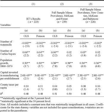
TSLS ANNUAL POPULATION GROWTH 1870–1900, BY COUNTY, USING POPULATION GROWTH FROM 1860 TO 1870 IN THE TWO-STAGE GROWTH MODEL WITH PREDICTED NUMBER OF CORLISS BUYERS IN THE FIRST STAGE (OLS AND POISSON MODELS)

**statistically significant at the 5 percent level.
*statistically significant at the 10 percent level.
Note:
All models included a constant term that was statistically insignificant in all cases. Coefficients for the state dummy variables are not included for space considerations, t-statistics are reported in the parentheses.
Starting with a sample of 242 counties that existed in 1880 in eleven eastern states having at least one of 257 petitioners supporting Corliss' application for patent renewal, RT drop a number of counties for their estimations. Table 1, column 1 shows RT's results for the second stage of the two-stage growth model using population growth from 1860 to 1870 as a regressor in the second stage and the OLS and the Poisson models in the first stage (columns 1a and 1b).Footnote 3 In this case, RT dropped Providence, RI (home of the Corliss engine), the highest growth county between 1850 and 1860, the highest growth county between 1870 and 1900, and sixteen counties missing population data for the year 1850 for a sample size of 223.
We determined that thirteen counties had no population data in 1850 because they were formed after 1850.Footnote 4 We are able to construct population data for these thirteen counties by using population data for the new and contributing counties from the first census year after the creation of the new counties. We estimate 1850 populations for both the new counties and the reduced-in-size contributing counties by assuming that the growth of the new counties and the reduced-in-size counties was the same as the growth of the contributing counties. We were able to find population data for all other counties giving us a full sample size of 242.
Although watermill data for 1870 is most appropriate for estimating growth in counties from 1870 to 1900, RT argue that 1880 data should be comparable to 1870 data and construct watermill data for 1880 drawing upon several sources. RT were unable to find watermill data for 25 percent of counties (about sixty counties) in 1880 and assumed that no watermills existed in these counties. We found 1880 watermill data for all but nineteen counties and, following RT, assume that no watermills existed in these counties. We also were able to find the more appropriate 1870 watermill data from the 1870 Census of Manufacturers. We report results using our expanded 1880 data. Results using our 1870 data for watermills are similar.
Since we have more complete data, we begin our replication attempts using all 242 counties. Following RT, we delete Providence and the highest growth county from 1860 to 1870 and the highest growth county between 1870 and 1900. Column 2 reports our results based on this sample of 239. While the coefficients for both models are essentially identical to those of RT shown in column 1, the Corliss coefficient is statistically significant at the 5 percent level only when using OLS in the first-stage estimation.Footnote 5 As another robustness test, if we exclude the thirteen newly formed counties along with Providence and two high-growth outliers for a sample size of 226, the Corliss coefficient is still statistically significant (now at the lower 10 percent level) but only when the less appropriate OLS estimation is used in the first-stage estimation (Table 1, column 3).
The thirteen new counties and the twenty-one counties that supplied population to the new counties grew faster on average than other counties between 1870 and 1900. Only one of these counties had a Corliss buyer and it experienced negative population growth between 1870 and 1900. The counties with no Corliss buyers had annual population growth of 1.6 percent compared to the average growth for the other 207 counties of 1 percent. Given the atypical nature of these thirty-four counties, we also investigated the impact of excluding them along with Providence for a smaller sample size of 207. Dropping all these counties avoids the importance of making adjustments to population in 1850, not only for the contributing counties, but for the newly formed counties. The results for the sample of 207 (results not reported) are essentially the same as those with the sample of 239.
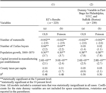
TSLS ANNUAL POPULATION GROWTH 1870–1900, BY COUNTY, USING 239 SAMPLE WITH AN ADDITIONAL CONTROL FOR LARGE PORTS

**statistically significant at the 5 percent level.
*statistically significant at the 10 percent level.
Note:
All models included a constant term that was statistically insignificant in all cases. Coefficients for the state dummy variables are not included for space considerations, t-statistics are reported in the parentheses.
Although not a part of RT's paper, we also explored the hypothesis that immigration, not the number of steam engines, drove urban growth by adding a dichotomous variable in the first stage with the value 1 if the county contained a major northeastern port (e.g., Suffolk (Boston), NYC, and Philadelphia).Footnote 6 This port-city dummy variable is significant in the first-stage estimation indicating that the port cities most subject to large immigration flows were magnets for Corliss steam engines. The Corliss coefficient now becomes insignificant even when OLS is used in the first stage (see Table 2, column 2).Footnote 7 This lends support for Kim's hypothesis that immigration, instead of steam engines, was a driving force for urban growth and casts more doubt about the independent role of Corliss steam engines.
CONCLUDING REMARKS
In summary, we are unable to replicate RT's main result for the effect of Corliss steam engines when using the preferred nonlinear first-stage estimation procedure. We are able to approach their result using some subsamples of counties and the less appropriate OLS first-stage estimation procedure. However, support for the Corliss effect even using the OLS procedure is highly sensitive to sample size and modification of the first-stage equation. These findings make us less sanguine about the independent role of Corliss steam engines in furthering county population growth. More positively, the other results reported by RT concerning the impact of watermills and prior population growth rates are robust and are not sensitive to these issues.