INTRODUCTION
In the profession, it has increasingly been recognized that formal modeling of monetary policy faces great challenges because of many kinds of uncertainties such as model uncertainty, shock uncertainty, and data uncertainty. Recent studies dealing with these uncertainties include Isard et al. (1999), Martin and Salmon (1999), Svensson (1999), Wieland (2000), Meyer et al. (2001), Tetlow and von zur Muehlen (2001a), Giannoni (2002), Orphanides and Williams (2002), and Söderström (2002).1
Several contributions to this problem can also be found in a recent issue of this journal [Giannoni (2002), Onatski and Stock (2002)].
For a study of the effect of model uncertainty in the context of ecological management problem, see Brock and Xepapadeas (2003).
Empirical work on parameter uncertainty and how to capture it by modeling and estimating parameter shifts can be found in Cogley and Sargent (2001), who study the inflation dynamics of the United States after WWII by way of Bayesian VAR with time-varying parameters without stochastic volatility. Yet, Sims (2001b) points out that the monetary policy behavior may not have experienced such a sharp change as shown by Cogley and Sargent (2001). Sims and Zha (2002) also study parameter shifts in estimates of the U.S. economy and find more evidence in favor of stable dynamics with unstable variance of the disturbance than of clear changes in model structure. In contrast to Sims (2001b), Cogley and Sargent (2003) study the drifts and volatilities of the U.S. monetary policy after WWII through a Bayesian VAR with time-varying parameters and stochastic volatility and claim to have found regime changes. Semmler et al. (2005) undertake a time-varying parameter estimation of the Phillips curve and Taylor rule by way of the Kalman filter and observe parameter shifts over time.
Thus, given such evidence on parameter and shock uncertainties, economic agents (central banks, for example) may resort to different strategies: They may either reduce uncertainty by learning or just seek a policy robust to model uncertainty without learning. As to the former, among the important research, the work by Sargent (1993, 1999) has attracted much attention. Although Sargent (1999) explores monetary policy rules with adaptive learning in an optimal control framework, he assumes that once the uncertain parameter is updated, the government pretends that the updated parameters will govern the dynamics forever. His analysis is undertaken in the traditional LQ framework. With such an approach, there may exist convergence to an ergodic distribution in a stochastic model and convergence with probability 1 in a non stochastic model. However, as mentioned by Tetlow and von zur Muehlen (2001b), the above problem in Sargent's assumption represents an inconsistency in his adaptive learning mechanism.
Because of this problem in Sargent's approach, it is a challenge to explore the learning algorithm in an appropriate manner. Therefore, in this paper, we study monetary policy rules under uncertainty with adaptive learning by using a dynamic programming algorithm recently developed by Grüne (1997) and Grüne and Semmler (2004). Our approach differs from Sargent's in that we are able to endogenize the learning of uncertain parameters and explore the problem with a dynamic-programming algorithm with adaptive grids which can deal with nonlinear constraints.
As stated above, the alternative for monetary authorities is to resort to a monetary policy rule robust to uncertainty. This is a strategy different from adaptive learning. In this approach the central bank considers the economic model only as an approximation to another model that it cannot specify. With a so-called robustness parameter, it pursues a monetary policy rule allowing for a worst-case scenario. Whereas adaptive learning considers mainly parameter uncertainty, robust control might consider more general uncertainties. The robustness parameter, as stated by Gonzalez and Rodriguez (2003), can be considered as a measure of uncertainty and may affect the robust monetary policy.
The important question concerning monetary policy under uncertainty is whether uncertainty requires caution. Brainard (1967), for example, proposes that parameter uncertainty should imply a more cautious policy. This argument has been supported by the recent research of Martin and Salmon (1999), who explore the monetary policy of the United Kingdom employing a VAR model with and without parameter uncertainty. They find that the optimal rule in the presence of parameter uncertainty implies a less aggressive path for official interest rates than when no parameter uncertainty is considered. However, other researchers—Gonzalez and Rodriguez (2003) and Giannoni (2002), for example—argue that uncertainty does not necessarily require caution. We also study this problem using robust control theory, obtaining results similar to those of Giannoni (2002).
The remainder of this paper is organized as follows: In the second section, we present empirical evidence on parameter and shock uncertainties in the IS and Phillips curves by way of a state-space model with Markov switching. In Section 3, we explore monetary policy rules under model uncertainty with adaptive learning. Section 4 explores monetary policy rules with robust control and Section 5 concludes the paper.
EMPIRICAL EVIDENCE OF UNCERTAINTY: A STATE-SPACE MODEL WITH MARKOV SWITCHING
Consider an economic model

subject to

where ρ is the discount factor bounded between 0 and 1, L(xt, ut) is a loss function of an economic agent (central bank, for instance), xt is a vector of state variables, ut is a vector of control variables, εt is a vector of shocks, and E0 denotes the mathematical expectation operator upon the initial values of the state variables. This kind of model represents the basic monetary control model employed by Clarida et al. (1999), Svensson (1997, 1999), and Beck and Wieland (2002), for example, where the constraint equations are usually IS and Phillips curves. Given the loss function L(x, u) and the state equation (2), the problem is to derive a path of the control variable, u, to satisfy (1). However, the question arising is whether the state equation (2) can be correctly specified with time-series estimates. The uncertainty of the state equation can be caused by the uncertainty in the shock εt and uncertainty in parameters and data. Svensson (1999) and Semmler et al. (2004) derive an optimal monetary policy rule from an optimal control problem similar to the model above and find that the optimal monetary policy rule is greatly affected by the estimated parameters of the model. Therefore, if the parameters in the model are uncertain, the derived optimal monetary policy rule may not be very reliable.
One can estimate time-varying parameters of the traditional Phillips curve with the following state-space model3
For further details of such a model, see Semmler et al. (2005).


where πt denotes the inflation rate and vt is a vector of the lags of the inflation rate and output gap. βt is a vector of time-varying parameters. Note that, in this model, it is assumed that the shocks have constant variance and only βt is uncertain. Cogley and Sargent (2001) study the inflation dynamics of the United States after WWII by way of a Bayesian VAR with time-varying parameters without stochastic volatility. Sims (2001b), however, claims that the monetary policy behavior may not have experienced such a sharp change as demonstrated by Cogley and Sargent (2001). Sims and Zha (2002) also study macroeconomic switching of the U.S. policy and find more evidence in favor of stable dynamics with unstable disturbance variance than of clear changes in model dynamics. Therefore, Cogley and Sargent (2003) modify the model by considering both time-varying parameters and stochastic volatility and claim to have found regime switching.
A drawback of the traditional state-space model such as (3) and (4) is that the changes of the time-varying parameters may be exaggerated because the shocks are assumed to have constant variance. This is the reason why Cogley and Sargent (2003) assume stochastic volatility. Therefore, in the research below, we assume that εt has state-dependent variance. This is similar to the assumption of Cogley and Sargent (2003). But unlike Cogley and Sargent (2003), who assume the variances of the shocks to change from period to period, we assume that there are only two states of disturbance variance with Markov property. This is, to some extent, similar to the assumption by Sims and Zha (2002) who assume that there are three states of economy. With such an assumption we can explore the probability of regime switching. Another advantage of the state-space model with Markov switching is that, as we will see below, it can explore not only parameter uncertainty but also shock uncertainty.
Following Kim and Nelson (1999), we simply assume that εt in (3) has two states of variance with Markov property,4
Vázquez (2003) estimates an augmented Taylor rule with a Markov-switching VAR model with the U.S. data of 1967–2002 and finds that there is no essential difference between the models with two regimes and three regimes and therefore, the model with two regimes can describe the economy well.

with

and

where St=0 or 1 indicates the states of the variance of εt and Pr stands for probability. In the research below, we explore uncertainty in the IS and Phillips curves since these two curves form the core of a monetary policy model.
We explore uncertainty in the traditional IS and Phillips curves which have often been taken as constraints in an optimal control model such as (1)–(2). To reduce the dimension of the model, we estimate the Phillips and IS curves with only one lag of the inflation rate and output gap:


where πt is the inflation rate, yt is the output gap, Rt is the short-term nominal interest rate, and επ,t and εy,t are shocks subject to Gaussian distributions with zero mean and Markov-switching variances.5
Forward-looking behaviors have been frequently taken into account in the Phillips curve. A survey of this problem can be found in Clarida et al. (1999). Because it is quite difficult to estimate a state-space model with forward-looking behaviors, we just consider backward-looking behaviors in this section. A justification of the above type of backward-looking model can be found in Rudebusch and Svensson (1999).


where Λt denotes the dependent variables (πt, yt) and Xt the independent variables (πt−1, yt−1 and rt−1); ϕt denotes the time-varying parameters αn,t and βn,t (n=1, 2, 3);
(St=0 or 1) is the drift of ϕt; and F is a diagonal matrix with constant elements to be estimated from the model; ηt has the distribution shown in equation (4); εt is now assumed to have the distribution presented in equation (5).6
Theoretically, the elements of F and the variance of ηt also may have a Markov property, but since there are already many parameters to estimate, we just ignore this possibility to improve the efficiency of estimation. Note that if the elements of F are larger than 1 in absolute value, that is, if the time-varying parameters are nonstationary, the transition equation should be altered to be the form of eq. (4).
As for the details of the state-space model with Markov switching, the reader is referred to Kim and Nelson (1999, Ch. 5). The program applied subsequently is based on the Gauss programs developed by Kim and Nelson (1999).
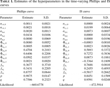
The estimation is undertaken with the quarterly U.S. data of 1964.1–2003.1. The inflation rate is measured by changes in the GDP deflator; the output gap is measured by the percentage deviation of the Industrial Production Index (IPI) from its fourth-order polynomial trend.8
The IPI has also been used by Clarida et al. (1998) to measure the output for Germany, France, the United States, the United Kingdom, Japan, and Italy. Clarida et al. (1998) use the quadratic trend of the IPI to measure the potential output for the United States of the period 1979–1993. We use the fourth-order trend of the IPI as the potential output because we cover a much longer period and the fourth-order trend fits the data better than the quadratic one. As surveyed by Orphanides and van Norden (2002), there are many approaches to measure the output gap.
(0.4704) and
(0.6406) is less significant than that between
(0.0502) and
(0.0021). The difference between
(0.0873) and
(−0.3364) is significant not only in magnitude and t-statistics but also in signs. Therefore, the estimation results confirm a state of economy with high volatility and a state with low volatility. The fact that all the elements of F are smaller than 1 in magnitude indicates that the time-varying parameters are stationary and, as a result, justifies the adoption of equation (9).

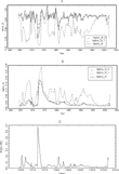
The paths of α2t are shown in Figure 1A. We leave aside the paths of the intercepts in the IS and Philips curves just for simplicity. Let Yt denote the vector of observations available as of time t. In Figure 1A, “Alpha_2t,0” and “Alpha_2t,1” denote the paths of α2t when [St=0|Yt] (α2t,0) and [St=1|Yt] (α2t,1), respectively. “Alpha_2t” denotes the weighted sum of α2t,0 and α2t,1, α2t. That is,

The paths of α3t are shown in Figure 1B. In Figure 1B, “Alpha_3t,0” and “Alpha_3t,1” denote the paths of α3t when [St=0|Yt] (α3t,0) and [St=1|Yt] (α3t,1) respectively. Similarly, “Alpha_3t” denotes the weighted sum of α3t,0 and α3t,1 (α3t). Figure 1C represents the path of Pr[St=1|Yt]. It is clear that the economy is probably in state 1 most of the time since Pr[St=1|Yt] is very high except at the beginning of the 1970s. Therefore, α2t is very close to α2t,1 and α3t is close to α3t,1 most of the time; α2t experienced some significant changes between 1970 and 1975 and at the beginning of the 1980s; α3t also experienced significant changes in the first half of the 1970s, increasing from about 0.02 to 0.20. We can also check these structural changes with the Chow breakpoint test of the following regression (t-statistics in parentheses):

with R2=0.979 and DW=2.026. The F-statistics of the Chow breakpoint test for 1971.4 and 1981.4 are 2.325 and 4.712, respectively, larger than the critique value at the 5% level of significance, which is between 2.26 and 2.29, implying structural changes around these two points.

Empirical evidence of uncertainty in the Phillips curve.
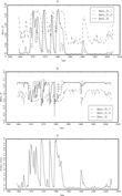
The estimation result of the IS curve is demonstrated in Figure 2. The paths of β2t and β3t are represented in Figure 2A and 2B, and Figure 2C, is the path of Pr[St=1|Yt]. From Figure 2C, we find that the IS curve was probably in state 1 before the beginning of the 1980s and in state 0 afterward. Therefore, β2t was close to β2t,1 before 1982 and close to β2t,0 afterward. The same is true of β3t. Both β2t and β3t experienced some significant structural changes in the 1970s and small changes around 1990. It is also obvious that the time-varying parameters show some structural changes at the beginning of the 1980s, which coincides with the beginning of the post-Volcker period. Then, after that, for the period from 1984 to 1990, the time-varying parameters seemed to be relatively stable.9
The differences of the monetary policy rules of the United States across periods have also been explored by Clarida et al. (2000).

Empirical evidence of uncertainty in the IS curve.
In the preceding, we have explored parameter and shock uncertainties in the IS and Phillips curves with the U.S. data. The results are consistent with the line of research that maintains that there were regime changes in the U.S. economy.10
Overall, the uncertainty of parameters and shocks and their impact on monetary policy rules suggest exploring monetary policy rules with learning and robust control.MONETARY POLICY RULES WITH ADAPTIVE LEARNING
The question arising is: What is the optimal monetary policy rule in case some parameters or shocks in an economic model as presented by equations (1)–(2) are uncertain? Recently, numerous papers have been contributed to this problem. Svensson (1999), Tetlow and von zur Muehlen (2001a), Beck and Wieland (2002), Orphanides and Williams (2002), Söderström (2002), and McGough (2003), for example, explore optimal monetary policy rules under the assumption that the economic agents learn the parameters in the model in a certain manner. One approach is that the economic agents may learn the parameters using the Kalman filter. This approach has been pursued by Tucci (1997) and Beck and Wieland (2002). Another learning mechanism that is also applied frequently is the recursive least-squares (RLS) algorithm. This kind of learning mechanism has been applied by Sargent (1999) and Orphanides and Williams (2002). By intuition, we would expect that economic agents reduce uncertainty and therefore improve economic models by learning over time, using all information available.
Beck and Wieland (2002) and Orphanides and Williams (2002) have explored monetary policy with adaptive learning. Besides the difference in the learning algorithm they use, another difference between Beck and Wieland (2002) and Orphanides and Williams (2002) is that the former do not consider the role of expectations in the model, whereas the latter take into account expectations in the Phillips curve. Unlike Beck and Wieland (2002), Orphanides and Williams (2002) do not employ an intertemporal framework. They provide a learning algorithm with constant gain but do not use a discounted loss function. Moreover, Orphanides and Williams (2002) assume that the government knows the true model, but the private agents do not know the true model and have to learn the parameters with the RLS algorithm. In their case the government and the private agents are treated differently.
Among the research of monetary policy with adaptive learning, the work of Sargent (1999) has attracted much attention. Sargent (1999) employs a learning algorithm as well as a discounted loss function, but in an LQ model. Yet, he constructs his results in two steps. First, assuming the RLS learning algorithm with a decreasing or constant gain, the agents estimate a model of the economy using the latest available data and update parameter estimates from period to period. Second, once the unknown parameter is updated, an optimal policy is derived from an LQ control model under the assumption that the updated parameter will govern the dynamics forever. As remarked by Tetlow and von zur Muehlen (2001b), however, the two steps are inconsistent with each other.
Because of this problem in Sargent's approach, it is required to explore such models by employing appropriate solution techniques. Therefore, in this section we will explore monetary policy with adaptive learning by using a recently developed dynamic programming algorithm.11
Evans and Honkapohja (2001) analyze expectations and learning mechanisms in macroeconomics in detail.
Thus, the difference of our model from that of Beck and Wieland (2002) can be summarized in three points: First, we consider both linear and nonlinear Phillips curves. Second, we take into account expectations. This is consistent with the model of Orphanides and Williams (2002). An important characteristic of New Keynesian economics is that current economic behavior depends not only on the current and past policy but also on the expectations of agents. Third, we employ the RLS learning algorithm instead of the Kalman filter. In fact, Harvey (1981) and Sargent (1999) prove that RLS is a specific form of the Kalman filter.
RLS Learning in a Linear Phillips Curve
Orphanides and Williams (2002) assume that the current inflation rate is not only affected by the inflation lag but also by inflation expectations. Following Orphanides and Williams (2002), we assume that the linear Phillips curve takes the following form:

where
denotes the agents' (including the central bank) expected inflation rate based on the time t−1 information, γ1, γ2 ∈ (0, 1), γ3>0; εt is a serially uncorrelated innovation. We further assume that the IS equation reads as:12
This is the same as Orphanides and Williams (2002), except that they assume a noise in the equation.

where rt denotes the deviation of the short-term real interest rate from its equilibrium level. Substituting equation (10) into (11), we have

In the case of rational expectations, namely,
, we get

that is,

with

With these results, we get the rational expectations equilibrium (REE)

Now, suppose that the agents believe the inflation rate follows the process

corresponding to the REE, but that a and b are unknown and have to be learned. Suppose that the agents have data on the economy from periods i=0, …, t−1. Thus the time-(t−1) information set is
. Further, suppose that agents estimate a and b by a least-squares regression of πi on πi−1 and ri−1. The estimates will be updated over time as more information is collected. Let (at−1, bt−1) denote the estimates through time t−1. The forecast of the inflation rate is then given by

The standard least-squares formula gives the equations

where zi=(πi−1 ri−1)′.
Defining

we can also compute equation (15) using the stochastic approximation of the recursive least-squares equations


where ct and Vt denote respectively, the coefficient vector and the moment matrix for zt using data i=1, …, t; κt is the gain. To generate the least-squares values, one must set the initial value for the recursion.13
Evans and Honkapohja (2001, Ch. 2, p. 33) p. n. 4 explain how to set the initial values of ct and Vt as follows. Assuming Zk=(z1, …zk)′ is of full rank and letting πk denote πk=(π1, …, πk)′, the initial value ck is given by
and the initial value Vk is given by
.
with probability 1, with
and therefore
REE.
As indicated by Sargent (1999) and Evans and Honkapohja (2001), if κt is a constant, however, there might be difficulties of convergence to the REE. If the model is nonstochastic and κt sufficiently small,
can converge under the condition γ2<1. However, if the model is stochastic with γ2<1, the belief does not converge to REE, but to an ergodic distribution around it. Here we follow Orphanides and Williams (2002) and assume that agents are constantly learning in a changing environment. The assumption of a constant gain implies that the agents believe the Phillips curve might exhibit structural changes and they allocate larger weights to the recent observations of the inflation rate than to the earlier ones. Orphanides and Williams (2002) denote the case of κt=1/t as infinite memory and the case of constant κt as finite memory. Following Svensson (1997, 1999) we assume that the central bank pursues a monetary policy by minimizing a quadratic loss function. The problem reads as

subject to equations (12), (14), (16), and (17); π* is the target inflation rate, which is assumed to be zero.14
To simplify the problem, we assume strict inflation targeting; that is, the central bank is concerned only with the inflation stabilization.
As mentioned above, if the unknown parameters are adaptively estimated with RLS learning with a small and constant gain, they will converge in distributions in a stochastic model and converge with probability 1 in a nonstochastic model. However, an optimal control problem such as (18) with nonlinear state equations, embedded in equations (12), (14), (16), and (17), is difficult to solve and, using appropriate solution techniques, indicates that the model will not necessarily converge even if the state equations are nonstochastic.
Next, we undertake an appropriate numerical study of the model. Though the return function is quadratic and the Phillips curve is linear, the problem falls outside the scope of LQ optimal control problems since some parameters in the Phillips curve are time varying and follow nonlinear paths. The problem cannot be solved analytically, and numerical solutions have to be employed. In the numerical study below, we resort to the algorithm developed by Grüne (1997), who applies adaptive rather than uniform grids.15
A less technical description and economic applications of this algorithm can be found in Grüne and Semmler (2004).
and only bt has to be learned in the model. In this case, we have ct=bt and zi=ri−1. As mentioned by Beck and Wieland (2002, p. 1361), the reason for focusing on the unknown parameter b is that “this parameter is multiplicative to the decision variable rt and therefore central to the trade-off between current control and estimation.”
Numerical Study
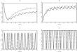
In the numerical study, undertaken by the above-mentioned dynamic programming algorithm, we assume γ1=0.6, γ2=0.4, γ3=0.5, θ=0.4, ρ=0.985, and κt=0.05. The initial values of πt, bt, and Vt are 0.2, −0.6, and 0.04. The paths of πt, bt, Vt, and rt are shown in Figures 3A–D, respectively. Figure 3E is the phase diagram of πt and rt. Neither the state variables nor the control variable converges. In fact, they fluctuate cyclically. We explore solution paths with many different initial values of the state variables and smaller κt (0.01, for example) and find that in no cases do the variables converge. Similar results are obtained with different values for γ1 (0.9 and 0.3, for example) and γ2 (0.1 and 0.7, for example).

Simulations of RLS learning (solid) and benchmark model (dashed) with linear Phillips curve.
With the parameters above, we have
,
; therefore, the REE of the stochastic version is

In the case of RLS learning, however, we have

with

If there is perfect knowledge with rational expectation, πt can converge to its target value π* (zero here) since the model then becomes a typical LQ control problem which has converging state and control variables in a nonstochastic model. We define this case as the benchmark model. The results of the benchmark model are shown in Figure 3A and 3D (dashed line). Note that the benchmark model contains only one state variable, namely πt, with dynamics denoted by (19). In this benchmark case, it is clear that the reaction function should be a linear function of the state variables. In the nonstochastic benchmark model, we find that the optimal monetary policy rule turns out to be rt=3.00πt and, substituting this into the deterministic version of equation (19) generates the optimal trajectory of πt, πt=0.01πt−1. It is obvious that in the steady state, we have πt=πt−1=0. From Figure 3A and 3D, we observe that πt and rt converge to zero over time in the benchmark model.
RLS Learning in Nonlinear Phillips Curve
We have explored adaptive learning in the context of a linear Phillips curve. The recent literature, however, argues that the Phillips curve might be nonlinear. Therefore, we next explore adaptive learning with a nonlinear Phillips curve.
As discussed by Aguiar and Martins (2002), there may be different forms of nonlinearity in the Phillips curve. Laxton et al. (1998) explore alternative shapes (concave, linear, and convex) of the U.S. Phillips curve and argue that the Fed should assume the convex form. More specifically, according to this literature, negative deviations of aggregate demand from potential are less disinflationary than positive deviations are inflationary. Therefore, we just follow Schaling (2002) and assume that the nonlinear form of the output gap in the Phillips curve reads as16
Note that this function is discontinuous at yt=1/(αβ). When yt<1/(αβ), f″(yt)>0 and if yt>1/(αβ), f″(yt)<0. In the research below, we choose appropriate values of α and β so that with the U.S. output gap data we have f″(yt)>0. In fact, this function can be shown to be a particular rational polynomial, as discussed by Escribano (2004). Escribano (2004) shows that any nonlinear function can be approximated by rational polynomials by employing Padé's approximants. Escribano (2004) also discusses some new rational-polynomial nonlinear error-correction models. The reader is referred to Escribano (2004, p. 81) for the details of rational polynomials and Padé's approximants.

where yt denotes the output gap, and the parameter β indexes the curvature of the curve. When β is very small, the curve approaches a linear relationship. Given the above nonlinear Phillips curve, equation (11) reads as

with f(yt) given by equation (21). Substituting equation (11) into equation (21), and then (21) into (22), we get the following nonlinear Phillips curve

where

The REE turns out to be

where
is the same as in the preceding subsection, but
is changed to be −γ3/(1−γ2). The forecast of the inflation rate is now given by

The RLS learning mechanism is the same as the case of the linear Phillips curve, except that zi is now modified as

The optimal control problem (18) now turns out to have constraints (23), (25), (16), and (17).
Numerical Study.
In this version, again using the aforementioned dynamic programming algorithm, we assume α=10 and β=0.99. The solution paths with the same starting values of the state variables as in the preceding subsection are presented in Figure 4A–D. Figure 4A represents the path of πt, 4B the path of bt, 4C the path of Vt, and 4D the path of rt. The results of this subsection (nonlinear Phillips curve) are presented by dashed lines, whereas the results from the preceding subsection (linear Phillips curve) are indicated by solid lines.17
To see the differences of the simulations clearly, we present only the results from t=6 onward.

RLS learning with linear (solid) and nonlinear Phillipscurves (dashed).
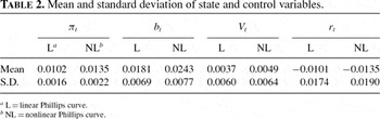
We find that the state variables also do not converge in the optimal control problem with the nonlinear Phillips curve. Similar to the case of the linear Phillips curve, the state and control variables fluctuate cyclically. Experiments with many different initial values of state variables were undertaken and in no cases are the state variables found to converge. However, the difference between the simulations with linear and nonlinear Phillips curves cannot be ignored. Figure 4 indicates that both πt (Figure 4A) and bt (Figure 4B) evolve at a higher level in the case of a nonlinear Phillips curve than in the case of a linear one. The mean and standard deviation of πt, bt, Vt, and rt from the two experiments are shown in Table 2. The standard deviation (S.D.) and magnitudes of the mean of these variables are larger in the case of the nonlinear Phillips curve than in the case of the linear one. As in the preceding subsection, the solutions are explored with different γ1 and γ2 and the results are similar.
The fact that the inflation rate has a higher mean and experiences larger changes in the nonlinear Phillips curve than in the linear one seems to be consistent with the research of Tambakis (1998) who analyzes the single-period Barro-Gordon optimal monetary problem with a convex Phillips curve and an asymmetric loss function. Tambakis (1998) finds that both symmetric and asymmetric loss functions with a convex Phillips curve yield a positive expected inflation bias. The reason is that, unlike the case of a quadratic loss function with a linear Phillips curve, in the case of a quadratic loss function with a convex Phillips curve, Eπ=π* does not necessarily satisfy the first-order condition. Therefore, inflation rate does not necessarily equal its target in equilibrium. This problem has also been analyzed by Graham and Snower (2002) and Karanassou and Snower (2003). They argue that the long-run Phillips curve might be nonvertical and the inflation rate might be different from its target in equilibrium, depending on the extent to which economic agents are forward or backward looking.

We have explored optimal monetary policy rules with adaptive learning. The simulations indicate that the state variables do not converge no matter whether the linear or nonlinear Phillips curve is employed. This is different from the work of Sargent (1999) because the state variables can converge in such a nonstochastic model with his approach. The problem in Sargent (1999), as mentioned before, is that he employs two assumptions which turn out to be inconsistent with each other. This is because he explores the problem in a traditional LQ framework, which fails to accurately endogenize the uncertain parameter. Our results are, however, consistent with the claim of Beck and Wieland (2002), who also find that the state variables do not converge even if all shocks in the stochastic model are set to zero, because economic agents never stop experimentation in each period.
MONETARY POLICY RULES WITH ROBUST CONTROL
A disadvantage of adaptive learning analyzed in the preceding section is that we have considered only parameter uncertainty. Monetary authorities have to guard against uncertainties such as model misspecification in a more general way. For this purpose, robust control theory has been applied. Robust control induces the economic agents to seek a strategy for the “worst case” and can deal with more general uncertainties than adaptive learning does. On the basis of some earlier papers [see Hansen and Sargent (1999, 2001a,b)], Hansen and Sargent (2002) explore robust control in macroeconomics in details. Cagetti et al. (2002) also employ robust control in macroeconomics. Svensson (2000) applies the idea of robust control in a simpler framework. Giordani and Söderlind (2003) and Giannoni (2002), however, extend the use of robust control theory by considering forward-looking behaviors.
The interesting question concerning monetary policy under uncertainty is whether the central bank should show a stronger or weaker response to the fluctuations of economic variables than when no uncertainty exists. Brainard (1967), for example, proposes that parameter uncertainty should incur a more cautious policy. This argument has been supported by recent research by Martin and Salmon (1999) who explore the monetary policy of the United Kingdom employing a VAR model with and without parameter uncertainty. They find that the optimal rule in the presence of parameter uncertainty incurs a less aggressive path for official interest rates than when no parameter uncertainty is considered. Other researchers, Gonzalez and Rodriguez (2003) and Giannoni (2002), for example, however, argue that uncertainty does not necessarily require caution. Following Hansen and Sargent (2002), in this section, we explore this problem with robust control and take up the problem of the control bank's response under uncertainty with respect to model misspecification.18
Brock et al. (2003) and Brock and Xepapadeas (2003) also explore policy in an uncertain economic environment. Whereas they have discussed how changes of parameters in a model may affect the policy response, here we discuss how the so-called robustness parameter may influence the policy rules.
The research undertaken below is based on the framework of Hansen and Sargent (2002). A short introduction to robust control theory is given in Appendix B. The so-called robustness parameter θ plays an important role in the problem's solution. If θ is +∞, the problem collapses to the traditional optimal control without model misspecification. Gonzalez and Rodriguez (2003) explore how the robustness parameter θ affects the control variable and prove that in a one-state, one-control model, the response is characterized by a hyperbolic function with a discontinuity at
. Such a response presents a concave shape on the right side of the discontinuity and a convex one on the left.
Related to the above is the concept of a detection-error probability. It is a statistic concept that can tell us how difficult it is to tell the approximating model apart from the distorted one. The larger the detection-error probability, the more difficult it is to tell the two models apart. The design and interpretation of the detection-error probability are shown in Appendix B.
Semmler et al. (2005) estimate the IS and Phillips curves with the U.S. quarterly data for the period 1961–1999.19
The data sources are OECD and IMF. The output gap is measured by the percent deviation of the IPI from its HP-filtered trend. The inflation rate is measured by the changes in the CPI, and the interest rate is the Federal Funds rate.

and ut=rt with πt, yt, and rt being the inflation rate, output gap, and deviation of the interest rate from its target (assumed to be zero in the simulation below), respectively. The problem then turns out to be

subject to

With the parameters above and the starting values of π0 and y0 both being 0.02, λ=1, ρ=0.985, and
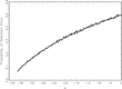
, the detection error probability is shown in Figure 5.20
The numerical studies in this section are done with the algorithms developed by Hansen and Sargent (2002). In the computation of the detection-error probability, T (number of periods) is 150 and 5,000 simulations are undertaken here.

Detection error probability.
With θ=0.03, we have

and the value function turns out to be V(π, y)=16.240 π2+1.033y2+1.421 πy+0.113. If we want a higher detection-error probability, 0.40, for example, we have σ=−11(θ=0.091),

and V(π, y)=11.134π2+1.022y2+0.945πy+0.080. In case θ=+∞,21
In the simulation, we just take
. In fact, the changes in the simulation results are too small to be observed if θ is a large number. Therefore, taking
can capture the simulation results of θ=+∞.
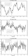
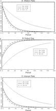
Next, we present the paths of the inflation-rate deviation, the output gap, and the interest rate with different θ in Figure 6A–C.

Simulation of the robust control with π0=0.02and y0=0.02.
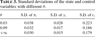
We find that the lower the θ is, the larger the volatility of the state and control variables. The standard deviations of the state and control variables are shown in Table 3, which indicates that the standard deviations of the state and control variables increase if θ decreases.22
Some researchers, Orphanides and Williams (2002), for example, assume that the loss function of the central bank is the weighted sum of the variances of output gap and inflation. In this case, the results of the numerical computation above implies that the smaller the θ, the higher the loss function.
Next, we come to a special case, namely, the case of zero shocks. What do the state and control variables look like and how can the robustness parameter θ affect the state variables and the objective function? According to the certainty equivalence principle, the optimal rules of the robust control with zero shocks are the same as when there are nonzero shocks. That is, F and K in equations (\ref{E:fdef}) and (\ref{E:kdef}) do not change whether there are shocks or not. The difference lies in the value function. The simulations for zero shocks and with the same parameters as the case of nonzero shocks are shown in Figure 7A–C. In Figure 7, we find that the state variables converge to their equilibria zero whether the robustness parameter is small or large. However, in case the robustness parameter is small, the state variables evolve at a higher level and converge more slowly to zero than when the robustness parameter is large. The simulations indicate that the larger the robustness parameter θ, the lower πt, yt, and rt and, moreover, the faster the state variables converge to their equilibria. In case θ=+∞, the state variables reach their lowest values and attain the equilibria at the highest speed.


Results of the robust control with zero shocks.
In sum, we have shown that uncertainty with respect to model misspecification might not necessarily require caution. Though robust control can deal with problems that cannot be solved with the classical optimal control theory, some researchers have casted doubt on robust control. Chen and Epstein (2000) and Epstein and Schneider (2001), for example, criticize the application of the robust control for time inconsistency in preferences. Therefore, Hansen and Sargent (2001b) discuss the time consistency of the alternative representations of preferences that underlie the robust control theory. An important criticism of robust control comes from Sims (2001a). He criticizes the robust control approach on conceptual grounds. Robust control also imposes neutrality properties of monetary policy implied in the model, which will not be removed by better local approximations. There are major sources of a more fundamental type of uncertainties that the robust control theory does not address.23
Moreover, steady states might not be optimal, if multiple steady states exist; see Greiner and Semmler (2002).
CONCLUSION
This paper is concerned with monetary policy rules under uncertainty. We first presented some evidence of uncertainty using a state-space model with Markov switching. The empirical model using the U.S. data indicates that there have been regime changes in both parameters and shocks. On the basis of this empirical evidence, we have then explored two approaches to deal with monetary policy under uncertainty: adaptive learning and robust control. In the former case the central bank is assumed to improve its knowledge of economic models by learning from the information available. Whereas the adaptive learning mainly considers parameter uncertainty, robust control admits more general uncertainties.
As to adaptive learning, in contrast to Sargent (1999), who explores monetary policy with adaptive learning in a two-step decision process, we have endogenized the uncertain parameter and employed a dynamic programming algorithm with adaptive grids, which can deal with nonlinear state equations, so that we have solved the model appropriately. With such an approach, we were able to overcome the problem of inconsistency in the two-step decision process of Sargent (1999). Yet, different from the work of Sargent (1999), we show that, when the learning of coefficients is fully endogenized, the state variables do not necessarily converge even in a nonstochastic model with adaptive learning.
As regards robust control, which is a more general approach to guard policy against uncertainty, we have focused on model misspecification and shock uncertainty and explored whether uncertainty requires caution. Different from the common view that monetary policy under uncertainty should be more cautious as compared to no uncertainty, our research indicates that the robust policy rule may respond more strongly to the economic variables in the presence of uncertainty and therefore implies that uncertainty does not necessarily require caution.
Finally, we note that there might exist other kinds of uncertainties, among which the data uncertainty has attracted much attention. The usually discussed data uncertainty is concerned with the output gap or Nairu uncertainty. A discussion of the unreliability of output gap estimated with real-time data can be found in Orphanides and van Norden (2002). The effect of data uncertainty on monetary policy may be different from the effects of model and shock uncertainties.25
Jenkins (2002) claims that the policy to be pursued may not be affected by pure data uncertainty in the case of additive-shock uncertainty. However, in case the central bank follows an interest-rate rule that is a function of a small number of variables, the monetary policy rule may be largely affected by data uncertainty.
Rudebusch (2001), for example, shows that an increase in output-gap uncertainty may reduce the coefficient on the output gap.
APPENDIX A: BRIEF SKETCH OF STATE-SPACE MODEL WITH MARKOV SWITCHING
Below is a brief sketch of the state-space model with Markov switching explored by Kim and Nelson (1999). Let Yt−1 be the vector of observations available at time t−1. In a traditional Kalman filter in a state-space model without Markov switching, the forecast of ϕt based on Yt−1 can be written as ϕt|t−1, and the matrix that denotes the mean squared error of the forecast reads

with E being the expectation operator.
In the state-space model with Markov switching, however, the forecast of ϕt is based on Yt−1, as well as on the random variable St taking on the value j and on St−1 taking on the value i (i and j equal 0 or 1):

The mean squared error of the forecast reads

Conditional on St−1=i and St=j (i, j=0, 1), the Kalman filter algorithm for our model is


where
is the conditional forecast error of Λt based on information up to time t−1 and
is the conditional variance of the forecast error \smash{
}. To make the above Kalman filter algorithm operable, Kim and Nelson (1999) develop some approximations and manage to collapse
and
into
and
, respectively.
Because the Phillips and IS curves contain only lags of variables and have uncorrelated noise, we can estimate the two equations separately. For the Phillips curve, we have the following state-space model:

with


and similarly for the IS curve, we have

with

APPENDIX B: BRIEF SKETCH OF ROBUST CONTROL
Below is a brief sketch of robust control theory explored by Hansen and Sargent (2002). Let the loss function be L(y, u)≡−(x′Qx+u′Ru), with Q being positive semidefinite and R positive definite matrices, respectively. The problem without model misspecification is

subject to the so-called approximating model27
The matrices A, B, Q, and R are assumed to satisfy the assumptions stated by Hansen and Sargent (2002, Ch. 3).

where
is an i.i.d. vector process subject to normal distribution with mean zero and identity covariance matrix. If there is model misspecification that cannot be depicted by
, Hansen and Sargent (2002) take a set of models surrounding equation (B.2) of the form (the so-called distorted model)

where {εt} is another i.i.d. process subject to normal distribution with mean zero and identity covariance matrix, and ωt+1 is a vector process that reads

with {gt} being a sequence of measurable functions. Hansen and Sargent (2002) further restrain the approximation errors by

to express the idea that equation (B.2) is a good approximation when equation (B.3) generates the data. To solve the robust control problem (B.1) subject to equations (B.3) and (B.5), Hansen and Sargent (2002) consider two kinds of robust control problems—the constraint problem and the multiplier problem—which differ in how they implement the constraint (B.5). The constraint problem is

subject to equations (B.3) and (B.5). Given θ ∈ (
, +∞) with
, the multiplier problem can be presented as

subject to equation (B.3). Hansen and Sargent (2002, Ch. 6) prove that under certain conditions the two problems have the same outcomes. Therefore, solving one of the two problems is sufficient.
The robustness parameter θ plays an important role in the problem's solution. If θ is +∞, the problem then becomes the usual optimal control problem without model misspecification. To find a reasonable value for θ, Hansen and Sargent (2002, Ch. 13) design a detection-error probability function by a likelihood ratio. Assume that there is a sample of observations from t=0 to t=T−1, and define Lij as the likelihood of this sample for model j, provided that the data are generated by model i. The likelihood ratio is then

Note that ri should be larger than zero if the data are generated by model i. Define

Assuming equal prior weights to both models, the detection-error probability can be defined as

When a reasonable value of p(θ) is chosen, a corresponding value of θ can be determined by inverting the probability function defined in (B.9). Hansen and Sargent (2002, Ch. 7) find that θ can be defined as the negative inverse value of the so-called risk-sensitivity parameter σ; that is, θ=−1/σ.
Note the interpretation of the detection-error probability. The larger the detection-error probability, the more difficult it is to tell the two models apart. So, a central bank can choose a θ according to how large a detection-error probability it wants. If the detection-error probability is very small, it is not necessary to design a robust rule. Note that the higher the θ, the lower the robustness, not the opposite.
The solution of the multiplier problem is shown below. Define


Let P be the fixed point of iterations on
:

Then, the solution of the multiplier problem (B.7) is


with


If θ=+∞,
, the problem above then becomes the traditional LQ problem.