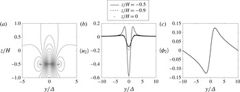
1 Introduction
The importance of mountain-generated inertia–gravity waves for the atmospheric circulation has long been recognised (see Fritts & Alexander Reference Fritts and Alexander2003, for a review), and their parameterisation is now an essential element of weather forecasting and climate models (e.g. Alexander et al. Reference Alexander, Geller, McLandress, Polavarapu, Preusse, Sassi, Sato, Eckermann, Ern and Hertzog2010). Their oceanic counterparts, while often neglected, are now increasingly thought to play a significant role for the oceanic circulation (e.g. Nikurashin & Ferrari Reference Nikurashin and Ferrari2011, Reference Nikurashin and Ferrari2013; Scott et al. Reference Scott, Goff, Garabato and Nurser2011). These waves impact both the atmospheric and oceanic circulations through the drag they exert where they dissipate, often through their interaction with the large-scale flow at critical levels where the mean flow velocity vanishes or, accounting for the background rotation, at inertial levels where their Doppler-shifted frequency matches the local Coriolis frequency.
Our understanding of this form of interaction with the mean flow rests on a number of now classical papers (including Eliassen & Palm Reference Eliassen and Palm1961; Bretherton Reference Bretherton1966, Reference Bretherton1969a ,Reference Bretherton b ; Booker & Bretherton Reference Booker and Bretherton1967; Jones Reference Jones1967) that tackled both the propagation of the waves in a shear flow and the drag they exert on the flow. These identified the Eliassen–Palm (EP) flux (or pseudomomentum flux) as the key quantity controlling the drag, showed that its conservation in the absence of dissipation leads to non-interaction results (Charney & Drazin Reference Charney and Drazin1961; Andrews & McIntyre Reference Andrews and McIntyre1976, Reference Andrews and McIntyre1978), and elucidated how critical-level and inertial-level singularities disrupt this conservation and result in drag. These results have subsequently been applied to a variety of mountain shapes and flows.
The present paper focusses on the case of a topographic profile with two well-separated horizontal scales, with small-scale oscillations modulated over a large envelope scale. Topographies of this form are assumed in atmospheric model parameterisations (Martin & Lott Reference Martin and Lott2007) and are natural for the ocean, e.g. in ridge regions. Our aim is to provide a detailed description of the wavepacket generated by a relatively weak flow whose Rossby number based on the envelope scale is small. The Rossby number based on the oscillation scale is however large enough for the waves to be vertically propagating (rather than evanescent) from the ground up. The flow considered is back sheared, decreasing linearly from a positive value at the ground to a zero-velocity critical level higher up. Such a monotonic decrease is not particularly realistic, since real flows are more typically non-monotonic and critical levels, e.g. in the middle atmosphere, are the result of shear reversals. However, the important wave dynamics that we intend to capture is localised around the inertial levels and unaffected by the details of the propagation below, which are well described by standard ray tracing.
Background rotation is crucial in two respects for the problem considered: first, it contributes to the dispersion relation; second, it determines the nature of the singularities in the vertical structure of the wave solution. Specifically, rotation resolves the degeneracy of the critical-level singularity, which is independent of wavenumber, into a pair of wavenumber-dependent inertial levels. As a result, the singularities associated with the broad wavenumber spectrum of a wavepacket are smeared out over a range of altitude – the inertial layer – and the wavepacket solution itself is smooth in the limit of vanishing dissipation (Shutts Reference Shutts2001). (An analogous effect arises when the orientation of the flow changes with altitude, see Shutts (Reference Shutts1995, Reference Shutts2003).)
We tackle the three essential aspects of the problem by computing (i) the shape of the wavepacket, (ii) the associated EP flux and (iii) the mean-flow change that results from the divergence of this EP flux. We take advantage of the assumption of small Rossby number and of a related assumption of large Richardson number to carry out the entire computation asymptotically, relying on the Wentzel–Kramers–Brillouin (WKB) form of the vertical structure of plane waves in the horizontal obtained by Lott, Plougonven & Vanneste (Reference Lott, Plougonven and Vanneste2010, Reference Lott, Plougonven and Vanneste2012). The analysis identifies two distinct altitude ranges corresponding to two distinct asymptotic regimes. In the first, valid away from the inertial levels, standard ray tracing applies and the (horizontally integrated) EP flux is independent of altitude; in the second, valid in a thin region surrounding the inertial layer, the solution is more complicated and captures the finiteness of the wavepacket deflection as it approaches a central inertial level. It turns out that inertial-level absorption affects only a still thinner region, which defines an inertial layer. The mean drag is vertically localised in this layer.
The asymptotic approach provides answers to basic questions – such as the horizontal distance between mountain and region of wave drag, and the extent of this region – as scaling laws in terms of key parameters characterising the stratification, shear and mountain shape. These scaling relations, which likely apply to more general set-ups than the one we consider, may prove useful for the representation of mountain–wave drag in numerical models. We also emphasise that our approach provides a fully consistent treatment of wave–mean-flow interaction in a non-symmetric set-up, with small-scale averaging replacing the more familiar zonal averaging. This is in contrast with the earlier, heuristic treatment of Martin & Lott (Reference Martin and Lott2007).
The structure of this paper is as follows. We formulate the problem in § 2 and approximate the form of the wavepacket in different regimes using a steepest-descent method in § 3. In § 4 we use this approximation to calculate the EP flux and solve a mean quasi-geostrophic potential-vorticity equation to obtain the mean-flow response. We summarise and discuss our results in § 5.
2 Formulation
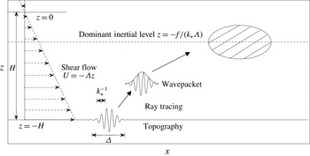
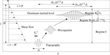
We consider the interaction between a steady topographic wavepacket and a background shear flow in an idealised set-up shown in figure 1. The background flow is chosen as a unidirectional, uniform backward shear flow
 $\boldsymbol{U}=(-\unicode[STIX]{x1D6EC}z,0,0)$
with
 $\unicode[STIX]{x1D6EC}=\text{const.}>0$
. The distance between the level of zero background velocity (critical level) and the bottom boundary is
 $H$
. It proves convenient to use a slightly unusual vertical coordinate such that
 $z=0$
and
 $z=-H$
correspond to the critical level and ground, respectively. The topographic wavepacket is generated by an idealised multiscale mountain with height
 $$\begin{eqnarray}\displaystyle h_{t}(x,y) & = & \displaystyle h\text{Re}(\text{e}^{-(x^{2}+y^{2})/(2\unicode[STIX]{x1D6E5}^{2})}\text{e}^{\text{i}\boldsymbol{k}_{\ast }\boldsymbol{\cdot }\boldsymbol{x}})\nonumber\\ \displaystyle & = & \displaystyle \frac{\unicode[STIX]{x1D6E5}^{2}h}{2\unicode[STIX]{x03C0}}\text{Re}\left(\int _{-\infty }^{\infty }\int _{-\infty }^{\infty }\text{e}^{-|\boldsymbol{k}-\boldsymbol{k}_{\ast }|^{2}\unicode[STIX]{x1D6E5}^{2}/2}\text{e}^{\text{i}\boldsymbol{k}\boldsymbol{\cdot }\boldsymbol{x}}\,\text{d}k\,\text{d}l\right),\end{eqnarray}$$
where
 $\boldsymbol{x}=(x,y)$
,
 $\boldsymbol{k}=(k,l)$
,
 $\boldsymbol{k}_{\ast }=(k_{\ast },l_{\ast })$
is the dominant wavevector,
 $h$
is the maximum height of the mountain, and
 $\text{Re}$
denotes the real part. Here
 $k_{\ast }^{-1}$
and
 $\unicode[STIX]{x1D6E5}$
control the oscillation scale and envelope scale of the mountain so that the parameter
 $k_{\ast }\unicode[STIX]{x1D6E5}\gg 1$
characterises the separation between these scales.
Schematic representation of the set-up of the problem in the
 $(x,z)$
-plane. A wavepacket generated by a two-scale mountain at the ground
 $z=-H$
propagates vertically in the shear flow
 $\boldsymbol{U}=(-\unicode[STIX]{x1D6EC}z,0)$
and drives a mean-flow in the (hatched) region localised around the dominant inertial level
 $z=-f/(k_{\ast }\unicode[STIX]{x1D6EC})$
.

The fluid satisfies the
 $f$
-plane hydrostatic Boussinesq equations
 $$\begin{eqnarray}\displaystyle & \displaystyle \unicode[STIX]{x2202}_{t}\boldsymbol{u}+\boldsymbol{u}\boldsymbol{\cdot }\unicode[STIX]{x1D735}\boldsymbol{u}+w\unicode[STIX]{x2202}_{z}\boldsymbol{u}+f\boldsymbol{e}_{z}\times \boldsymbol{u}=-\unicode[STIX]{x1D735}\unicode[STIX]{x1D719}, & \displaystyle\end{eqnarray}$$
 $$\begin{eqnarray}\displaystyle & \displaystyle \unicode[STIX]{x2202}_{z}\unicode[STIX]{x1D719}=b, & \displaystyle\end{eqnarray}$$
 $$\begin{eqnarray}\displaystyle & \displaystyle \unicode[STIX]{x2202}_{t}b+\boldsymbol{u}\boldsymbol{\cdot }\unicode[STIX]{x1D735}b+w\unicode[STIX]{x2202}_{z}b+N^{2}w=0, & \displaystyle\end{eqnarray}$$
 $$\begin{eqnarray}\displaystyle & \displaystyle \unicode[STIX]{x1D735}\boldsymbol{\cdot }\boldsymbol{u}+\unicode[STIX]{x2202}_{z}w=0, & \displaystyle\end{eqnarray}$$
 $\boldsymbol{u}=(u,v)$
is the horizontal velocity,
 $w$
the vertical velocity,
 $\unicode[STIX]{x1D719}$
a scaled pressure,
 $b$
the buoyancy,
 $f$
the local Coriolis frequency,
 $\boldsymbol{e}_{z}$
the unit vertical vector pointing upwards,
 $N$
the Brunt–Väisälä frequency, taken to be a constant, and
 $\unicode[STIX]{x1D735}=(\unicode[STIX]{x2202}_{x},\unicode[STIX]{x2202}_{y})$
is the horizontal gradient.
We apply a no-normal-flow boundary condition at the lower boundary:
 $$\begin{eqnarray}\displaystyle w=\boldsymbol{u}_{b}\boldsymbol{\cdot }\unicode[STIX]{x1D735}h_{t}\quad \text{at }z=-H+h_{t}, & & \displaystyle\end{eqnarray}$$
where the subscript ‘
 $b$
’ denotes the value on the boundary.
3 Wave solution
3.1 Preliminaries
We examine small-amplitude waves governed by the linearisation of the primitive equations (2.2)–(2.3) about the background flow. This is in geostrophic balance and given by
 $$\begin{eqnarray}\displaystyle U_{0}=-\unicode[STIX]{x2202}_{y}\unicode[STIX]{x1D6F9}_{0},\quad V_{0}=0,\quad W_{0}=0,\quad B_{0}=f\unicode[STIX]{x2202}_{z}\unicode[STIX]{x1D6F9}_{0},\quad \unicode[STIX]{x1D6F7}_{0}=f\unicode[STIX]{x1D6F9}_{0},\quad \text{where }\unicode[STIX]{x1D6F9}_{0}=\unicode[STIX]{x1D6EC}yz. & & \displaystyle \nonumber\\ \displaystyle & & \displaystyle\end{eqnarray}$$
We assume a small Rossby number based on the envelope scale
 $\unicode[STIX]{x1D6E5}$
of the topography:
 $$\begin{eqnarray}\displaystyle Ro=\frac{U_{b}}{f\unicode[STIX]{x1D6E5}}\ll 1, & & \displaystyle\end{eqnarray}$$
where
 $U_{b}=\unicode[STIX]{x1D6EC}H$
. We also assume that
 $NH/(f\unicode[STIX]{x1D6E5})=O(1)$
, corresponding to an order-one Burger number based on the horizontal and vertical scales
 $\unicode[STIX]{x1D6E5}$
and
 $H$
. Together with (3.2), this implies a large Richardson number, specifically
 $$\begin{eqnarray}\displaystyle J=\frac{N}{\unicode[STIX]{x1D6EC}}=O(Ro^{-1})\gg 1, & & \displaystyle\end{eqnarray}$$
where we have introduced the parameter
 $J=Ri^{1/2}$
as a convenient substitute for the Richardson number
 $Ri$
.
We are interested in mountain waves, in the distinguished regime where the Doppler-shifted frequency
 $U_{b}k_{\ast }$
is of the same order as the Coriolis frequency. This corresponds to the scaling
 $$\begin{eqnarray}\displaystyle r=\frac{U_{b}k_{\ast }}{f}=O(1), & & \displaystyle\end{eqnarray}$$
with
 $r$
a Rossby number based on the mountain wavelength rather than the envelope scale that appears in
 $Ro$
. Since
 $r=k_{\ast }\unicode[STIX]{x1D6E5}Ro$
, this implies that
 $$\begin{eqnarray}\displaystyle k_{\ast }\unicode[STIX]{x1D6E5}=O(Ro^{-1})\gg 1. & & \displaystyle\end{eqnarray}$$
To ensure that the waves are propagating rather than evanescent at the bottom boundary we further require that
 $$\begin{eqnarray}\displaystyle r>1. & & \displaystyle\end{eqnarray}$$
We emphasise that the scaling specified by (3.2), (3.3) and (3.5) corresponds to a distinguished limit, that is, it leads to results valid for a broad range of relative values of
 $Ro$
,
 $J$
and
 $k_{\ast }\unicode[STIX]{x1D6E5}$
. This becomes apparent in the asymptotic derivation of § 3.2 and is discussed further in the Conclusion, § 5.
Linearising (2.2) around the background flow (3.1) leads to the equations
 $$\begin{eqnarray}\displaystyle & \displaystyle \unicode[STIX]{x2202}_{t}\boldsymbol{u}_{1}-\unicode[STIX]{x1D6EC}z\unicode[STIX]{x2202}_{x}\boldsymbol{u}_{1}+\unicode[STIX]{x1D6EC}w_{1}\boldsymbol{e}_{x}+f\boldsymbol{e}_{z}\times \boldsymbol{u}_{1}=-\unicode[STIX]{x1D735}\unicode[STIX]{x1D719}_{1}, & \displaystyle\end{eqnarray}$$
 $$\begin{eqnarray}\displaystyle & \displaystyle \unicode[STIX]{x2202}_{z}\unicode[STIX]{x1D719}_{1}=b_{1}, & \displaystyle\end{eqnarray}$$
 $$\begin{eqnarray}\displaystyle & \displaystyle \unicode[STIX]{x2202}_{t}b_{1}-\unicode[STIX]{x1D6EC}z\unicode[STIX]{x2202}_{x}b_{1}+f\unicode[STIX]{x1D6EC}v_{1}+N^{2}w_{1}=0, & \displaystyle\end{eqnarray}$$
 $$\begin{eqnarray}\displaystyle & \displaystyle \unicode[STIX]{x1D735}\boldsymbol{\cdot }\boldsymbol{u}_{1}+\unicode[STIX]{x2202}_{z}w_{1}=0, & \displaystyle\end{eqnarray}$$
 $\boldsymbol{e}_{x}$
the unit vector in the
 $x$
-direction, which govern the leading-order wave fields, denoted here by the subscript ‘1’. The amplitude of the waves is determined by the linearisation of the boundary condition (2.3) around the background flow (3.1),
 $$\begin{eqnarray}\displaystyle w_{1}=U_{b}\unicode[STIX]{x2202}_{x}h_{t}. & & \displaystyle\end{eqnarray}$$
This indicates that
 $w_{1}=O(U_{b}k_{\ast }h)$
. The polarisation relation for standard internal waves (see also (3.14a
) below) can then be used to estimate
 $u_{1}=O(Nw_{1}/(k_{\ast }U_{b}))=O(Nh)$
. The linearisation based on the small-amplitude condition
 $u_{1}\ll U_{b}$
thus requires that the inverse Froude number be small:
 $$\begin{eqnarray}\displaystyle \frac{Nh}{U_{b}}=J\frac{h}{H}\ll 1. & & \displaystyle\end{eqnarray}$$
Based on this small parameter, we introduce the convention of using a subscript ‘
 $n$
’
 $(n=1,2,3\ldots \,)$
to denote the
 $n$
th-order flow variables such that
 $$\begin{eqnarray}\displaystyle u_{n}=O\left(\left(J\frac{h}{H}\right)^{n}U_{b}\right). & & \displaystyle\end{eqnarray}$$
After applying a Fourier transform, (3.7) can be reduced to the single equation
 $$\begin{eqnarray}\displaystyle \frac{1-\unicode[STIX]{x1D701}^{2}}{\unicode[STIX]{x1D701}^{2}}{\hat{w}}_{\unicode[STIX]{x1D701}\unicode[STIX]{x1D701}}-\left(\frac{2}{\unicode[STIX]{x1D701}^{3}}-\frac{2\text{i}\unicode[STIX]{x1D708}}{\unicode[STIX]{x1D701}^{2}}\right){\hat{w}}_{\unicode[STIX]{x1D701}}-\left(\frac{(1+\unicode[STIX]{x1D708}^{2})J^{2}}{\unicode[STIX]{x1D701}^{2}}+\frac{2\text{i}\unicode[STIX]{x1D708}}{\unicode[STIX]{x1D701}^{3}}\right){\hat{w}}=0, & & \displaystyle\end{eqnarray}$$
where
 $\unicode[STIX]{x1D708}=l/k$
. (This is equation (25) in Jones (Reference Jones1967) and equation (4) in Yamanaka & Tanaka (Reference Yamanaka and Tanaka1984).) The independent variable is the scaled vertical coordinate
 $$\begin{eqnarray}\displaystyle \unicode[STIX]{x1D701}=-k\unicode[STIX]{x1D6EC}z/f. & & \displaystyle\end{eqnarray}$$
We emphasise that for
 $k>0$
, as will be assumed when interpreting the results,
 $\unicode[STIX]{x1D701}$
has a sign opposite to that of
 $z$
and is positive below the inertial level and increasing downwards. The dependent variable
 ${\hat{w}}$
is the horizontal Fourier transform of
 $w_{1}$
, defined by
 $$\begin{eqnarray}\displaystyle w_{1}(x,y,z)=\frac{1}{2\unicode[STIX]{x03C0}}\int _{-\infty }^{\infty }\int _{-\infty }^{\infty }{\hat{w}}(k,l,z)\text{e}^{\text{i}\boldsymbol{k}\boldsymbol{\cdot }\boldsymbol{x}}\,\text{d}k\,\text{d}l. & & \displaystyle\end{eqnarray}$$
The other dependent variables are related to
 ${\hat{w}}$
through the polarisation relations
 $$\begin{eqnarray}\displaystyle & \displaystyle \hat{u} =\text{i}\frac{-\unicode[STIX]{x1D6EC}}{f}\left(\frac{\unicode[STIX]{x1D701}-\text{i}\unicode[STIX]{x1D708}}{\unicode[STIX]{x1D701}(1+\unicode[STIX]{x1D708}^{2})}{\hat{w}}_{\unicode[STIX]{x1D701}}+\frac{\unicode[STIX]{x1D708}^{2}}{\unicode[STIX]{x1D701}(1+\unicode[STIX]{x1D708}^{2})}{\hat{w}}\right), & \displaystyle\end{eqnarray}$$
 $$\begin{eqnarray}\displaystyle & \displaystyle \hat{v}=\frac{\unicode[STIX]{x1D6EC}}{f}\left(\frac{1-\text{i}\unicode[STIX]{x1D708}\unicode[STIX]{x1D701}}{\unicode[STIX]{x1D701}(1+\unicode[STIX]{x1D708}^{2})}{\hat{w}}_{\unicode[STIX]{x1D701}}+\frac{\text{i}\unicode[STIX]{x1D708}}{\unicode[STIX]{x1D701}(1+\unicode[STIX]{x1D708}^{2})}{\hat{w}}\right), & \displaystyle\end{eqnarray}$$
 $$\begin{eqnarray}\displaystyle & \displaystyle \hat{b}=\text{i}\frac{\unicode[STIX]{x1D6EC}^{2}}{f}\left(\frac{1-\text{i}\unicode[STIX]{x1D708}\unicode[STIX]{x1D701}}{\unicode[STIX]{x1D701}^{2}(1+\unicode[STIX]{x1D708}^{2})}{\hat{w}}_{\unicode[STIX]{x1D701}}+\left(\frac{\text{i}\unicode[STIX]{x1D708}}{\unicode[STIX]{x1D701}^{2}(1+\unicode[STIX]{x1D708}^{2})}+\frac{J^{2}}{\unicode[STIX]{x1D701}}\right){\hat{w}}\right). & \displaystyle\end{eqnarray}$$
One of the key characteristics of inertia–gravity waves (IGWs) in shear flow is the presence of singularities: two inertial levels, where the Doppler-shifted frequency matches the Coriolis frequency, and a critical level, where the Doppler-shifted frequency and hence the background velocity vanish (Jones Reference Jones1967). These singularities are readily identified from (3.11): the two inertial levels and one critical level correspond to
 $\unicode[STIX]{x1D701}=\pm 1$
and
 $\unicode[STIX]{x1D701}=0$
, respectively. The critical level is an apparent singularity that can be removed by a variable transformation. The inertial levels, by contrast, have a marked physical impact since the wave solution switches abruptly from an oscillatory to an evanescent behaviour and back across them (Yamanaka & Tanaka Reference Yamanaka and Tanaka1984; Lott, Millet & Vanneste Reference Lott, Millet and Vanneste2015). As we discuss in § 4, this abrupt change underpins the forcing of a mean flow by the wavepacket.
Rotation plays a crucial role. The position
 $z=\pm f/(k\unicode[STIX]{x1D6EC})$
of the inertial levels depends on the wavenumber
 $k$
; as a result, the singularities associated with each wavenumber making up the wavepacket are smeared out over a range of altitude, and the wavepacket solution is smooth even in the absence of dissipation (or more precisely in the limit of vanishing dissipation since dissipation is important to determine physically relevant branches of solution; Shutts Reference Shutts2001). This is in contrast with the non-rotating scenario, best thought of as the limit
 $f\rightarrow 0$
of the general situation. In this limit, the inertial levels coalesce with the critical level, leading to a stronger,
 $k$
-independent singularity and to a singular behaviour of the wavepacket unless dissipation is introduced. (A similar smearing out of singularities across different altitudes also occurs without rotation when more complicated flows, such as the directional shear flow, are considered; Shutts Reference Shutts1995, Reference Shutts2003, Martin & Lott Reference Martin and Lott2007.)
The term ‘inertial layer’ is used to describe the region where the effect of the inertial-level singularities is distributed. It is centred around the dominant inertial level,
 $$\begin{eqnarray}\displaystyle z_{\ast }=-\frac{f}{k_{\ast }\unicode[STIX]{x1D6EC}}, & & \displaystyle\end{eqnarray}$$
determined by the central wavenumber
 $k_{\ast }$
of the topography. Note that, for the problem under consideration, only the lower inertial levels matter since the waves are exponentially small in
 $J$
at the upper inertial levels. Condition (3.6) ensures that
 $z_{\ast }>-H$
, that is, the dominant inertial level lies in the fluid domain. The characteristic thickness of the inertial layer is found as
 $$\begin{eqnarray}\displaystyle \unicode[STIX]{x1D6FF}_{\ast }=-\frac{z_{\ast }}{k_{\ast }}\unicode[STIX]{x1D6FF}k=\frac{f}{k_{\ast }^{2}\unicode[STIX]{x1D6EC}\unicode[STIX]{x1D6E5}}, & & \displaystyle\end{eqnarray}$$
on using that, according to expression (2.1) for the mountain height, the spectral width of the wavepacket is
 $\unicode[STIX]{x1D6FF}k=\unicode[STIX]{x1D6E5}^{-1}$
.
Equation (3.11) for
 ${\hat{w}}$
can be solved explicitly in terms of hypergeometric functions (Yamanaka & Tanaka Reference Yamanaka and Tanaka1984; Shutts Reference Shutts2001). We rely instead on the approximate WKB solution derived in Lott et al. (Reference Lott, Plougonven and Vanneste2012) (see also Lott et al.
Reference Lott, Millet and Vanneste2015) and valid in the large Richardson number limit
 $J\gg 1$
. In this solution,
 ${\hat{w}}$
is approximated as
 $$\begin{eqnarray}\displaystyle {\hat{w}}(k,l,z)=\frac{\unicode[STIX]{x1D701}}{\unicode[STIX]{x1D701}_{b}}\left(\frac{\unicode[STIX]{x1D701}_{b}-1}{\unicode[STIX]{x1D701}-1}\right)^{1/4-\text{i}\unicode[STIX]{x1D708}/2}\left(\frac{\unicode[STIX]{x1D701}_{b}+1}{\unicode[STIX]{x1D701}+1}\right)^{1/4+\text{i}\unicode[STIX]{x1D708}/2}\text{e}^{-\text{i}J\sqrt{1+\unicode[STIX]{x1D708}^{2}}D(\unicode[STIX]{x1D701})}, & & \displaystyle\end{eqnarray}$$
where
 $$\begin{eqnarray}\displaystyle D(\unicode[STIX]{x1D701})=\ln (\unicode[STIX]{x1D701}+\sqrt{\unicode[STIX]{x1D701}^{2}-1})-\ln (\unicode[STIX]{x1D701}_{b}+\sqrt{\unicode[STIX]{x1D701}_{b}^{2}-1}),\quad \text{with }\unicode[STIX]{x1D701}_{b}=k\unicode[STIX]{x1D6EC}H/f. & & \displaystyle\end{eqnarray}$$
Note that we have normalised
 ${\hat{w}}$
so that its bottom boundary value is
 ${\hat{w}}(\unicode[STIX]{x1D701}_{b})=1$
.
Expression (3.17) holds for all real values of
 $\unicode[STIX]{x1D701}$
except in small regions of
 $O(J^{-2})$
thickness around the inertial levels
 $\unicode[STIX]{x1D701}=\pm 1$
. The sign of the argument of the exponential is taken to be negative because this ensures that the wave is propagating upwards above the upper inertial level, that is, for
 $\unicode[STIX]{x1D701}<-1$
(see Booker & Bretherton (Reference Booker and Bretherton1967); note that the opposite, positive sign is found when the background velocity is increasing with altitude). The fractional powers and logarithms involved in (3.17) are multivalued functions for which suitable branches need to be selected. This selection is dictated by causality and is most easily settled by adding small damping terms in (3.7). The upshot is that the multivalued functions should be continued from
 $\unicode[STIX]{x1D701}<-1$
to
 $\unicode[STIX]{x1D701}>1$
along a contour in the complex plane that passes below the singularities at
 $\unicode[STIX]{x1D701}=\pm 1$
(Booker & Bretherton Reference Booker and Bretherton1967; Jones Reference Jones1967; Lott et al.
Reference Lott, Millet and Vanneste2015). In this way,
 $\sqrt{\unicode[STIX]{x1D701}^{2}-1}=-\text{i}\sqrt{1-\unicode[STIX]{x1D701}^{2}}$
between the inertial levels so that the solution is decreasing exponentially with
 $\unicode[STIX]{x1D701}$
there, like
 $\exp (-J\sqrt{1+\unicode[STIX]{x1D708}^{2}}\cos ^{-1}\unicode[STIX]{x1D701})$
. Overall, the solution experiences an absorption by the factor
 $\exp (-J\sqrt{1+\unicode[STIX]{x1D708}^{2}}\unicode[STIX]{x03C0})$
(see also Lott et al.
Reference Lott, Plougonven and Vanneste2012) known to apply to both the rotating and non-rotating cases. Note that the reliance on causality means that the problem is not treated as strictly inviscid but rather as a vanishing viscosity limit.
The WKB approximation (3.17) breaks down near the inertial levels, specifically for
 $||\unicode[STIX]{x1D701}|-1|=O(J^{-2})$
where it should be replaced by an expression in terms of Hankel functions (Lott et al.
Reference Lott, Plougonven and Vanneste2012). These regions are narrow enough and the singularities of (3.17) at
 $\unicode[STIX]{x1D701}=\pm 1$
are mild enough that they can be ignored when computing the vertical velocity of the complete wavepacket.
Substituting the form (2.1) of the topography into the boundary condition (3.8), we obtain the vertical velocity at the boundary as the Fourier expansion
 $$\begin{eqnarray}\displaystyle w_{1b}=\frac{\text{i}U_{b}h\unicode[STIX]{x1D6E5}^{2}}{2\unicode[STIX]{x03C0}}\int _{-\infty }^{\infty }\int _{-\infty }^{\infty }k\text{e}^{-|\boldsymbol{k}-\boldsymbol{k}_{\ast }|^{2}\unicode[STIX]{x1D6E5}^{2}/2}\text{e}^{\text{i}\boldsymbol{k}\boldsymbol{\cdot }\boldsymbol{x}}\,\text{d}k\,\text{d}l. & & \displaystyle\end{eqnarray}$$
Here and henceforth, a real part is implied. Combining this with (3.13) and (3.17) leads to the vertical velocity of the wavepacket in the form
 $$\begin{eqnarray}\displaystyle w_{1}=\frac{\text{i}U_{b}h\unicode[STIX]{x1D6E5}^{2}}{2\unicode[STIX]{x03C0}}\int _{-\infty }^{\infty }\int _{-\infty }^{\infty }k\text{e}^{-|\boldsymbol{k}-\boldsymbol{k}_{\ast }|^{2}\unicode[STIX]{x1D6E5}^{2}/2}{\hat{w}}\,\text{e}^{\text{i}\boldsymbol{k}\boldsymbol{\cdot }\boldsymbol{x}}\,\text{d}k\,\text{d}l. & & \displaystyle\end{eqnarray}$$
Note that, because
 ${\hat{w}}$
is exponentially small for
 $\unicode[STIX]{x1D701}<1$
as a result of wave absorption, the lower limit of the integral in
 $k$
could be taken as
 $-f\unicode[STIX]{x1D6EC}^{-1}z^{-1}$
. This absorption is crucial for the impact of the wavepacket on the mean flow.
3.2 Saddle-point approximations
The solution (3.20) can be further simplified by taking advantage of the assumptions
 $J\gg 1$
and
 $k_{\ast }\unicode[STIX]{x1D6E5}\gg 1$
to apply a saddle-point approximation. The key is to identify the dominant terms in the argument of the exponential, including a contribution from
 ${\hat{w}}$
. To avoid defining several new dimensionless numbers measuring the relative size of
 $J$
,
 $k_{\ast }\unicode[STIX]{x1D6E5}$
and
 $Ro$
, it is expedient to introduce a bookkeeping parameter
 $\unicode[STIX]{x1D716}$
which keeps track of the orders of various terms. This parameter is treated as formally small and used as a basis for a saddle-point approximation, but it is set to
 $1$
at the end of the computation to obtain asymptotic formulas in a convenient dimensional form. The bookkeeping parameter
 $\unicode[STIX]{x1D716}$
is introduced through the replacements
 $$\begin{eqnarray}\displaystyle \boldsymbol{k}_{\ast }\unicode[STIX]{x1D6E5}\mapsto \unicode[STIX]{x1D716}^{-1}\boldsymbol{k}_{\ast }\unicode[STIX]{x1D6E5},\quad J\mapsto \unicode[STIX]{x1D716}^{-1}J\quad \text{and}\quad Ro\mapsto \unicode[STIX]{x1D716}Ro, & & \displaystyle\end{eqnarray}$$
in accordance with the scalings (3.2), (3.3) and (3.5). Thus the formal smallness of
 $\unicode[STIX]{x1D716}$
captures at once the mountain scale separation, the large Richardson number, and the small Rossby number. We emphasise that the bookkeeping device is completely equivalent to using, say,
 $J$
as a large parameter and treating
 $\boldsymbol{k}_{\ast }\unicode[STIX]{x1D6E5}/J$
and
 $JRo$
as order one; it is employed here for the economy and transparency of notation it brings.
Introducing (3.21) into (3.20) leads to
 $$\begin{eqnarray}\displaystyle w_{1}=\frac{\text{i}U_{b}hk_{\ast }\unicode[STIX]{x1D6E5}^{2}}{2\unicode[STIX]{x03C0}\unicode[STIX]{x1D716}}\int _{-\infty }^{\infty }\int _{-\infty }^{\infty }\text{e}^{-|\boldsymbol{k}-\unicode[STIX]{x1D716}^{-1}\boldsymbol{k}_{\ast }|^{2}\unicode[STIX]{x1D6E5}^{2}/2}{\hat{w}}\text{e}^{\text{i}\boldsymbol{k}\boldsymbol{\cdot }\boldsymbol{x}}\,\text{d}k\,\text{d}l, & & \displaystyle\end{eqnarray}$$
where
 $$\begin{eqnarray}\displaystyle {\hat{w}}=\frac{\unicode[STIX]{x1D701}}{\unicode[STIX]{x1D701}_{b}}\left(\frac{\unicode[STIX]{x1D701}_{b}-1}{\unicode[STIX]{x1D701}-1}\right)^{1/4-\text{i}\unicode[STIX]{x1D708}/2}\left(\frac{\unicode[STIX]{x1D701}_{b}+1}{\unicode[STIX]{x1D701}+1}\right)^{1/4+\text{i}\unicode[STIX]{x1D708}/2}\text{e}^{-\text{i}\unicode[STIX]{x1D716}^{-1}J\sqrt{1+\unicode[STIX]{x1D708}^{2}}D(\unicode[STIX]{x1D701})}, & & \displaystyle\end{eqnarray}$$
and makes the dependence on
 $\unicode[STIX]{x1D716}$
explicit. In writing this expression, we have made a first approximation by replacing the wavenumber
 $k$
outside the exponential functions by its leading-order approximation
 $k_{\ast }$
. The error introduced is negligible as can be verified below once the size of the neighbourhood of
 $k_{\ast }$
controlling the integral is estimated.
A second approximation is made in carrying out the integration with respect to
 $l$
in (3.22). Because the integral is dominated by values of
 $l$
near
 $\unicode[STIX]{x1D716}^{-1}l_{\ast }$
, we write
 $$\begin{eqnarray}\displaystyle l=\unicode[STIX]{x1D716}^{-1}l_{\ast }+L, & & \displaystyle\end{eqnarray}$$
where
 $\unicode[STIX]{x1D716}L/l_{\ast }\ll 1$
, leading to the following expressions
 $$\begin{eqnarray}\displaystyle & \displaystyle \unicode[STIX]{x1D708}=\frac{l_{\ast }}{\unicode[STIX]{x1D716}k}\left(1+\unicode[STIX]{x1D716}\frac{L}{l_{\ast }}\right), & \displaystyle\end{eqnarray}$$
 $$\begin{eqnarray}\displaystyle & \displaystyle \sqrt{1+\unicode[STIX]{x1D708}^{2}}=\sqrt{1+\left(\frac{l_{\ast }}{\unicode[STIX]{x1D716}k}\right)^{2}}+\unicode[STIX]{x1D716}\frac{l_{\ast }L}{\unicode[STIX]{x1D716}k\sqrt{(\unicode[STIX]{x1D716}k)^{2}+l_{\ast }^{2}}}+O\left(\left(\unicode[STIX]{x1D716}\frac{L}{l_{\ast }}\right)^{2}\right), & \displaystyle\end{eqnarray}$$
where
 $\unicode[STIX]{x1D716}k$
is treated as
 $O(1)$
since
 $k$
is close to
 $\unicode[STIX]{x1D716}^{-1}k_{\ast }$
. Substituting these into (3.22) and neglecting
 $O((\unicode[STIX]{x1D716}L/l_{\ast })^{2})$
, we obtain
 $$\begin{eqnarray}\displaystyle w_{1} & = & \displaystyle \frac{\text{i}U_{b}hk_{\ast }\unicode[STIX]{x1D6E5}^{2}}{2\unicode[STIX]{x03C0}\unicode[STIX]{x1D716}}\int _{-\infty }^{\infty }\int _{-\infty }^{\infty }\exp (-(\unicode[STIX]{x0394}L)^{2}/2-\text{i}Jl_{\ast }(\unicode[STIX]{x1D716}k)^{-1}((\unicode[STIX]{x1D716}k)^{2}+l_{\ast }^{2})^{-1/2}D(\unicode[STIX]{x1D701})L+\text{i}Ly)\,\text{d}L\nonumber\\ \displaystyle & & \displaystyle \times \,\exp (-(k-\unicode[STIX]{x1D716}^{-1}k_{\ast })^{2}\unicode[STIX]{x1D6E5}^{2}/2)\frac{\unicode[STIX]{x1D701}}{\unicode[STIX]{x1D701}_{b}}\left(\frac{\unicode[STIX]{x1D701}_{b}-1}{\unicode[STIX]{x1D701}-1}\right)^{1/4-\text{i}\unicode[STIX]{x1D708}_{\ast }/2}\left(\frac{\unicode[STIX]{x1D701}_{b}+1}{\unicode[STIX]{x1D701}+1}\right)^{1/4+\text{i}\unicode[STIX]{x1D708}_{\ast }/2}\nonumber\\ \displaystyle & & \displaystyle \times \,\exp (-\text{i}J\unicode[STIX]{x1D716}^{-1}(1+l_{\ast }^{2}/(\unicode[STIX]{x1D716}k)^{2})^{1/2}D(\unicode[STIX]{x1D701})+\text{i}kx)\,\text{d}k\nonumber\\ \displaystyle & \doteq & \displaystyle \frac{U_{b}hk_{\ast }\unicode[STIX]{x1D6E5}}{\unicode[STIX]{x1D716}\sqrt{2\unicode[STIX]{x03C0}}}\int _{-\infty }^{\infty }\exp (-(y-Jl_{\ast }(\unicode[STIX]{x1D716}k)^{-1}((\unicode[STIX]{x1D716}k)^{2}+l_{\ast }^{2})^{-1/2}D(\unicode[STIX]{x1D701}))^{2}/(2\unicode[STIX]{x1D6E5}^{2}))\nonumber\\ \displaystyle & & \displaystyle \times \,\exp (-(k-\unicode[STIX]{x1D716}^{-1}k_{\ast })^{2}\unicode[STIX]{x1D6E5}^{2}/2)\frac{\unicode[STIX]{x1D701}}{\unicode[STIX]{x1D701}_{b}}\left(\frac{\unicode[STIX]{x1D701}_{b}-1}{\unicode[STIX]{x1D701}-1}\right)^{1/4-\text{i}\unicode[STIX]{x1D708}_{\ast }/2}\left(\frac{\unicode[STIX]{x1D701}_{b}+1}{\unicode[STIX]{x1D701}+1}\right)^{1/4+\text{i}\unicode[STIX]{x1D708}_{\ast }/2}\nonumber\\ \displaystyle & & \displaystyle \times \,\exp (-\text{i}J\unicode[STIX]{x1D716}^{-1}(1+l_{\ast }^{2}/(\unicode[STIX]{x1D716}k)^{2})^{1/2}D(\unicode[STIX]{x1D701})+\text{i}kx)\,\text{d}k.\end{eqnarray}$$
In the second line, we have ignored a phase factor and introduced the symbol
 $\doteq$
to denote an equality in modulus only, ignoring phase factors. In what follows, we pay only attention to the modulus of
 $w_{1}$
since this controls the wave–mean-flow interaction properties: the spatially averaged EP flux, which is quadratic in wave quantities, only depends on the wave amplitude and on the relative phase of various fields which is easily worked out.
The appearance of the bookkeeping parameter
 $\unicode[STIX]{x1D716}^{-1}$
in the exponential in (3.27) motivates the saddle-point approximation. To apply this, we need to compare the leading terms in the exponential, namely
 $$\begin{eqnarray}\displaystyle (k-\unicode[STIX]{x1D716}^{-1}k_{\ast })^{2}\unicode[STIX]{x1D6E5}^{2}/2\quad \text{and}\quad \text{i}J\unicode[STIX]{x1D716}^{-1}\left(1+\left(\frac{l_{\ast }}{\unicode[STIX]{x1D716}k}\right)^{2}\right)^{1/2}D(\unicode[STIX]{x1D701}). & & \displaystyle\end{eqnarray}$$
The first term stems from the finite spectral width of the mountain height; the second term, which depends on
 $\unicode[STIX]{x1D701}$
and hence
 $z$
, captures the vertical structure of the wave. We seek distinguished regimes, where the leading-order terms in (3.28) balance. This requires approximating
 $D(\unicode[STIX]{x1D701})$
to determine its order, a non-trivial task since the order of
 $D(\unicode[STIX]{x1D701})$
depends on the value of
 $\unicode[STIX]{x1D701}$
, that is, on the particular range of altitude considered. Mathematically, different altitude ranges are captured by different values of
 $\unicode[STIX]{x1D6FC}$
in the scaling
 $$\begin{eqnarray}\displaystyle z=z_{\ast }\left(1+\left(\frac{\unicode[STIX]{x1D716}}{k_{\ast }\unicode[STIX]{x1D6E5}}\right)^{\unicode[STIX]{x1D6FC}}Z\right), & & \displaystyle\end{eqnarray}$$
where
 $Z=O(1)$
.
Note that, since
 $z_{\ast }<0$
,
 $Z$
and
 $z$
have different signs, with
 $Z>0$
below the dominant inertial level and increasing downwards. Because
 $\unicode[STIX]{x1D701}$
depends on both
 $z$
and
 $k$
, we also need to scale
 $k$
to find range of wavenumbers controlling the integral in (3.27). Since the wavepacket is concentrated around
 $\unicode[STIX]{x1D716}^{-1}k_{\ast }$
, we write
 $$\begin{eqnarray}\displaystyle k=\unicode[STIX]{x1D716}^{-1}k_{\ast }\left(1+\left(\frac{\unicode[STIX]{x1D716}}{k_{\ast }\unicode[STIX]{x1D6E5}}\right)^{\unicode[STIX]{x1D6FD}}K\right),\quad \text{with }K=O(1)\text{ and }\unicode[STIX]{x1D6FD}\geqslant 0. & & \displaystyle\end{eqnarray}$$
Combining (3.29) and (3.30), we obtain
 $$\begin{eqnarray}\displaystyle \unicode[STIX]{x1D701}=-\frac{k\unicode[STIX]{x1D6EC}z}{f}=1+\left(\frac{\unicode[STIX]{x1D716}}{k_{\ast }\unicode[STIX]{x1D6E5}}\right)^{\unicode[STIX]{x1D6FD}}K+\left(\frac{\unicode[STIX]{x1D716}}{k_{\ast }\unicode[STIX]{x1D6E5}}\right)^{\unicode[STIX]{x1D6FC}}Z+O\left(\left(\frac{\unicode[STIX]{x1D716}}{k_{\ast }\unicode[STIX]{x1D6E5}}\right)^{\unicode[STIX]{x1D6FC}+\unicode[STIX]{x1D6FD}}\right). & & \displaystyle\end{eqnarray}$$
We now need to distinguish two situations: (i) for
 $\unicode[STIX]{x1D6FC}=0$
, that is, away from the dominant inertial level,
 $$\begin{eqnarray}\displaystyle D(\unicode[STIX]{x1D701})=D(1+Z)+O\left(\left(\frac{\unicode[STIX]{x1D716}}{k_{\ast }\unicode[STIX]{x1D6E5}}\right)^{\unicode[STIX]{x1D6FD}}\right); & & \displaystyle\end{eqnarray}$$
(ii) for
 $\unicode[STIX]{x1D6FC}>0$
, that is, asymptotically close to the dominant inertial level,
 $$\begin{eqnarray}\displaystyle D(\unicode[STIX]{x1D701})=D(1)+O\left(\left(\frac{\unicode[STIX]{x1D716}}{k_{\ast }\unicode[STIX]{x1D6E5}}\right)^{min\{\unicode[STIX]{x1D6FC},\unicode[STIX]{x1D6FD}\}/2}\right). & & \displaystyle\end{eqnarray}$$
Because the leading-order terms in these two expansions are independent of
 $k$
, hence do not contribute to the integration over
 $k$
in (3.27), the order of the second terms is crucial. Using the scalings of the second terms of (3.32)–(3.33) in the second expression in (3.28), and balancing with the first expression (scaling like
 $\unicode[STIX]{x1D716}^{2\unicode[STIX]{x1D6FD}-2}$
) leads to two distinguished regimes: Regime I, with
 $\unicode[STIX]{x1D6FC}=0$
and
 $\unicode[STIX]{x1D6FD}=1$
, and Regime II, with
 $\unicode[STIX]{x1D6FC}=\unicode[STIX]{x1D6FD}=2/3$
(since
 $\unicode[STIX]{x1D6FC}=\unicode[STIX]{x1D6FD}$
gives a distinguished regime). In each regime, the coordinate
 $x$
appearing in
 $\exp (\text{i}kx)$
should be scaled so that the
 $K$
-dependent contribution to
 $kx$
, proportional to
 $\unicode[STIX]{x1D716}^{\unicode[STIX]{x1D6FD}-1}$
, be of the same order as the
 $K$
-dependent terms in (3.28). This leads to
 $x=O(\unicode[STIX]{x1D6E5})$
in Regime I and
 $x=O(\unicode[STIX]{x1D716}^{-1/3}\unicode[STIX]{x1D6E5})$
in Regime II.
We carry out the saddle-point expansion of (3.27) in these two regimes in appendix A and only quote the final results here. In Regime I, after setting
 $\unicode[STIX]{x1D716}=1$
, we find that
 $$\begin{eqnarray}\displaystyle w_{1}\doteq hf(1+Z_{I})\left(\frac{r^{2}-1}{2Z_{I}+Z_{I}^{2}}\right)^{1/4}\exp (-(y-J\unicode[STIX]{x1D708}_{\ast }{k_{\ast }}^{-1}(1+\unicode[STIX]{x1D708}_{\ast }^{2})^{-1/2}D_{I})^{2}/(2\unicode[STIX]{x1D6E5}^{2}))\text{e}^{-X_{I}^{2}/(2\unicode[STIX]{x1D6E5}^{2})}, & & \displaystyle \nonumber\\ \displaystyle & & \displaystyle\end{eqnarray}$$
where
 $$\begin{eqnarray}\displaystyle X_{I}=x-\frac{J}{k_{\ast }}\left(\sqrt{1+\unicode[STIX]{x1D708}_{\ast }^{2}}\left(\frac{1+Z_{I}}{\sqrt{2Z_{I}+Z_{I}^{2}}}-\frac{r}{\sqrt{r^{2}-1}}\right)-\frac{\unicode[STIX]{x1D708}_{\ast }^{2}}{\sqrt{1+\unicode[STIX]{x1D708}_{\ast }^{2}}}D_{I}\right), & & \displaystyle\end{eqnarray}$$
 $D_{I}=\ln (1+Z_{I}+\sqrt{2Z_{I}+Z_{I}^{2}})-\ln (r+\sqrt{r^{2}-1})$
,
 $Z_{I}=z/z_{\ast }-1$
and we have used that
 $r=k_{\ast }\unicode[STIX]{x1D6EC}H/f$
. This makes clear that the wavepacket retains the bell shape of topography, with scale
 $\unicode[STIX]{x1D6E5}$
, throughout its propagation across Regime I. The path of the wavepacket in the
 $(x,z)$
-plane is determined by setting
 $X_{I}=0$
in (3.34), which corresponds to standard ray tracing. It shows in particular that the wavepacket diverges to infinity as it approaches the dominant inertial level, with
 $x\sim Jk_{\ast }^{-1}(1+\unicode[STIX]{x1D708}_{\ast }^{2})^{1/2}(2Z_{I})^{-1/2}$
as
 $Z_{I}\rightarrow 0$
. This is a limitation of the approximation made in Regime I (also a limitation of ray tracing) rather than a physical effect as the analysis of Regime II shows.
In Regime II, and again with
 $\unicode[STIX]{x1D716}=1$
, we find that
 $$\begin{eqnarray}\displaystyle w_{1}\doteq \frac{U_{b}hk_{\ast }^{2}\unicode[STIX]{x1D6E5}}{2^{1/4}(k_{\ast }\unicode[STIX]{x1D6E5})^{3/4}}\frac{q(K_{s})}{(p^{\prime \prime }(K_{s}))^{1/2}}\text{e}^{(k_{\ast }\unicode[STIX]{x1D6E5})^{2/3}p(K_{s})}g(y), & & \displaystyle\end{eqnarray}$$
where the
 $y$
-dependence is controlled by the Gaussian
 $$\begin{eqnarray}\displaystyle g(y)=\exp (-(y-J\unicode[STIX]{x1D708}_{\ast }{k_{\ast }}^{-1}(1+\unicode[STIX]{x1D708}_{\ast }^{2})^{-1/2}D_{II})^{2}/(2\unicode[STIX]{x1D6E5}^{2})), & & \displaystyle\end{eqnarray}$$
with
 $D_{II}=-\ln (r+\sqrt{r^{2}-1})$
, and is decoupled from the dependence in
 $x$
and
 $z$
. In (3.36), the function
 $p$
is defined by
 $$\begin{eqnarray}\displaystyle p(K_{s})=-\frac{K_{s}^{2}}{2}-\text{i}J(k_{\ast }\unicode[STIX]{x1D6E5})\sqrt{1+\unicode[STIX]{x1D708}_{\ast }^{2}}\sqrt{2(K_{s}+Z_{II})}+\text{i}K_{s}X_{II}, & & \displaystyle\end{eqnarray}$$
and
 $K_{s}$
is one of its saddle points, satisfying
 $p^{\prime }(K_{s})=0$
, where the prime denotes derivative. The other symbols introduced are
 $$\begin{eqnarray}\displaystyle & \displaystyle q(K_{s})=\frac{1}{(K_{s}+Z_{II})^{1/4}}, & \displaystyle\end{eqnarray}$$
 $$\begin{eqnarray}\displaystyle & \displaystyle X_{II}=(k_{\ast }\unicode[STIX]{x1D6E5})^{-4/3}\left(k_{\ast }x+J\left(\frac{r\sqrt{1+\unicode[STIX]{x1D708}_{\ast }^{2}}}{\sqrt{r^{2}-1}}+\frac{\unicode[STIX]{x1D708}_{\ast }^{2}}{\sqrt{1+\unicode[STIX]{x1D708}_{\ast }^{2}}}D_{II}\right)\right), & \displaystyle\end{eqnarray}$$
and
 $Z_{II}=(k_{\ast }\unicode[STIX]{x1D6E5})^{2/3}(z/z_{\ast }-1)$
. The saddle point
 $K_{s}$
satisfies a cubic equation whose analytic solution is not particularly illuminating; we will solve it numerically. It is selected among the three roots of the cubic by the condition that it be accessible by a steepest-descent path connecting
 $-\infty$
to
 $\infty$
(e.g. Bender & Orszag Reference Bender and Orszag1999). For large
 $Z_{II}$
, the expansion
 $\sqrt{2(K_{s}+Z_{II})}\sim \sqrt{2Z_{II}}+K_{s}/\sqrt{2Z_{II}}$
can be used to confirm the matching between Regime I and Regime II. The behaviour for small
 $Z_{II}$
is key for the mean-flow forcing. As discussed in § 3.1, the change in EP flux is concentrated in the inertial layer, such that
 $|z-z_{\ast }|=O(\unicode[STIX]{x1D6FF}_{\ast })$
with
 $\unicode[STIX]{x1D6FF}_{\ast }$
given in (3.16). This corresponds to the scaling
 $$\begin{eqnarray}\displaystyle Z=\unicode[STIX]{x1D716}^{-1}k_{\ast }\unicode[STIX]{x1D6E5}\left(\frac{z}{z_{\ast }}-1\right)=O(1), & & \displaystyle\end{eqnarray}$$
hence to
 $\unicode[STIX]{x1D6FC}=1$
in (3.29) and thus
 $Z_{II}=O(\unicode[STIX]{x1D716}^{1/3})\ll 1$
. For this range of
 $Z$
, the integral in (3.27) is dominated by wavenumbers
 $k$
in an
 $O(1)$
neighbourhood of the central wavenumber
 $\unicode[STIX]{x1D716}^{-1}k_{\ast }$
, corresponding to
 $\unicode[STIX]{x1D6FD}=1$
in (3.30). The associated regime, which we term Regime II
 $_{B}$
, is a limit of Regime II, obtained when some terms are negligible (notably the first term in the phase function (3.38)). This makes it possible to derive an expression for
 $w_{1}$
simpler than (3.36) which we will subsequently use to compute the mean-flow forcing. This expression is derived in § A.3 and given by
 $$\begin{eqnarray}\displaystyle w_{1}\doteq \frac{hfJ^{1/2}(1+\unicode[STIX]{x1D708}_{\ast }^{2})^{1/4}(r^{2}-1)^{1/4}}{(k_{\ast }\unicode[STIX]{x1D6E5})^{1/2}X}\text{e}^{-(a^{2}/X^{2}-Z)^{2}/2}g(y), & & \displaystyle\end{eqnarray}$$
where
 $$\begin{eqnarray}\displaystyle a=\frac{J\sqrt{1+\unicode[STIX]{x1D708}_{\ast }^{2}}}{\sqrt{2}k_{\ast }\unicode[STIX]{x1D6E5}} & & \displaystyle\end{eqnarray}$$
and
 $$\begin{eqnarray}\displaystyle X=(k_{\ast }\unicode[STIX]{x1D6E5})^{-3/2}\left(k_{\ast }x+J\left(\frac{r\sqrt{1+\unicode[STIX]{x1D708}_{\ast }^{2}}}{\sqrt{r^{2}-1}}+\frac{\unicode[STIX]{x1D708}_{\ast }^{2}}{\sqrt{1+\unicode[STIX]{x1D708}_{\ast }^{2}}}D_{II}\right)\right). & & \displaystyle\end{eqnarray}$$
According to this, the wavepacket is centred on the curve
 $$\begin{eqnarray}\displaystyle X=X_{c}=\left(\frac{J^{2}(1+\unicode[STIX]{x1D708}_{\ast }^{2})}{(k_{\ast }\unicode[STIX]{x1D6E5})^{2}(Z+\sqrt{2+Z^{2}})}\right)^{1/2} & & \displaystyle\end{eqnarray}$$
in the
 $(X,Z)$
-plane (obtained by maximising (3.42)) and localised in a region of order-one size in both the
 $X$
and
 $Z$
direction. In view of (3.41) and (3.44), this corresponds to a region of streamwise extent
 $O((k_{\ast }\unicode[STIX]{x1D6E5})^{1/2}\unicode[STIX]{x1D6E5})$
, thus much larger than the size
 $\unicode[STIX]{x1D6E5}$
of the mountain, located an
 $O((k_{\ast }\unicode[STIX]{x1D6E5})^{1/2}\unicode[STIX]{x1D6E5})$
distance downstream of the topography, and of
 $O(\unicode[STIX]{x1D6FF}_{\ast })$
vertical extent. Thus, the prediction of ray tracing of a wavepacket that diverges to infinity as the dominant inertial level is approached is replaced in Regime II
 $_{B}$
(and hence in Regime II) by a large-but-finite horizontal shift. Note that in the limit of
 $f\rightarrow 0$
, the wavepacket propagates vertically with a vertical velocity that tends to zero as it approaches the critical level
 $z=0$
towards which the inertial levels coalesce, with
 $w_{1}\propto z^{1/2}$
as
 $z\rightarrow 0$
. This can be deduced from (3.34) by letting
 $r\rightarrow \infty$
and is consistent with a direct computation assuming
 $f=0$
. For a small-but-finite
 $f$
, however, there is an extremely thin inertial layer of size
 $O((k_{\ast }\unicode[STIX]{x1D6E5})^{-2}Ro^{-1}H)$
, in which the wavepacket experiences the horizontal displacement described by (3.44).
We remark that the three regimes identified by the saddle-point analysis can be interpreted physically. Regime I is the ray-tracing regime, which is unaffected by the singularities of the wave solution. Regime II is controlled by the singularity at the lower inertial level, and Regime II
 $_{B}$
is its part dominated by inertial-level absorption.
3.3 Numerical results
In this section, we compare the asymptotic predictions for
 $w_{1}$
with direct numerical computations of the integral in (3.27). We first take the parameters
 $$\begin{eqnarray}\displaystyle Ro=0.02,\quad k_{\ast }\unicode[STIX]{x1D6E5}=100,\quad l_{\ast }\unicode[STIX]{x1D6E5}=100,\quad J=100\quad \text{and}\quad \unicode[STIX]{x1D708}_{\ast }=1, & & \displaystyle\end{eqnarray}$$
so
 $r=k_{\ast }\unicode[STIX]{x1D6E5}Ro=2$
. A choice of physical parameters leading to these values is
 $N=1.4\times 10^{-2}~\text{s}^{-1}$
,
 $f=10^{-4}~\text{s}^{-1}$
,
 $\unicode[STIX]{x1D6EC}=1.4\times 10^{-4}~\text{s}^{-1}$
,
 $H=5~\text{km}$
,
 $\unicode[STIX]{x1D6E5}=3.5\times 10^{2}~\text{km}$
and
 $k_{\ast }=2.8\times 10^{-4}~\text{m}^{-1}$
. The weak shear and short wavelengths make this choice somewhat contrived, but it has the advantage of enabling a comparison in conditions where the asymptotic assumptions hold unambiguously. Parameters corresponding to a stronger shear and longer wavelengths are considered at the end of the section. We concentrate on the amplitude
 $|w_{1}|$
in the
 $(x,z)$
cross-section where it is maximum, since the structure in
 $y$
is simply the Gaussian structure of the mountain envelope, albeit with a shift.
Vertical velocity amplitude
 $|w_{1}|$
in the
 $(x,z)$
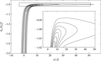
plane obtained by numerical integration of (3.22) for the parameters in (3.46) (7 equispaced contours with velocity in the range
 $[0.04,0.28]\times Uhk_{\ast }/\sqrt{2\unicode[STIX]{x03C0}}$
are shown). The inset is a zoom on the rectangle region indicated in the main panel.

Figure 2 shows a contour plot of
 $|w_{1}|$
obtained numerically. Away from the dominant inertial level,
 $k_{\ast }\unicode[STIX]{x1D6EC}z/f=-1$
, the wavepacket is only slightly deflected from the vertical. Closer to the dominant inertial level, the wavepacket shows a significant bend; we can read off from the inset that the peak of the wavepacket at the dominant inertial level is approximately
 $x/\unicode[STIX]{x1D6E5}\approx 12$
, in agreement with the peak value predicted in (3.44) which gives
 $X_{c}=2^{1/4}$
. This figure is more a qualitative illustration than a quantitative comparison which we carry out next.
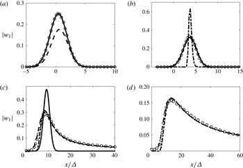
Vertical velocity amplitude
 $|w_{1}|$
normalised by
 $Uhk_{\ast }/\sqrt{2\unicode[STIX]{x03C0}}$
as a function of
 $x/\unicode[STIX]{x1D6E5}$
for the altitudes given by
 $-k_{\ast }\unicode[STIX]{x1D6EC}z/f=1.5$
(a), 1.05 (b), 1.01 (c) and 1 (d), and the parameters in (3.46). Numerical results (circles) are compared with the asymptotic predictions of Regime I (solid line, shown in panels a–c), Regime II (dashed line) and Regime II
 $_{B}$
(dash-dotted line, shown in panels b–d).

Figure 3 provides a detailed comparison of the numerical and asymptotic predictions for
 $|w_{1}|$
. Its four panels show
 $|w_{1}|$
as a function of
 $x/\unicode[STIX]{x1D6E5}$
at four different altitudes. Panel (a) corresponds to
 $-k_{\ast }\unicode[STIX]{x1D6EC}z/f=1.5$
, sufficiently far below the dominant inertial level for the Regime I asymptotics to apply. As expected, the asymptotic predictions of Regime I (solid line) matches the numerical results (circles), with a wavepacket that takes the bell shape of the mountain envelope, while the predictions of Regime II (dashed line) do not. Panel (b) shows the wavepacket closer to the dominant inertial level, for
 $-k_{\ast }\unicode[STIX]{x1D6EC}z/f=1.05$
, in a region where Regime I and Regime II overlap: the predictions of both regimes match the numerical results. The Regime II
 $_{B}$
approximation is also shown (dash-dotted line) and, unsurprisingly, is found to be invalid. Closer still to the dominant inertial level, as shown in panel (c) for
 $-k_{\ast }\unicode[STIX]{x1D6EC}z/f=1.01$
, the Regime I approximation breaks down. The Regime II predictions match the numerical results closely, while those of Regime II
 $_{B}$
are accurate for
 $x$
large enough. As expected, the wavepacket is no longer bell shaped, and its peak is shifted by an
 $O((k_{\ast }\unicode[STIX]{x1D6E5})^{1/2}\unicode[STIX]{x1D6E5})$
amount to the right (since
 $x/\unicode[STIX]{x1D6E5}\approx 10=(k_{\ast }\unicode[STIX]{x1D6E5})^{1/2}$
) in agreement with (3.44) and (3.45). Finally, at the dominant inertial level as shown in panel (d), the predictions of both Regime II and Regime II
 $_{B}$
coincide and match the numerical results in most of range of
 $x$
, except to the very left of the peak where Regime II
 $_{B}$
underestimates the amplitude. As discussed above, the peak of the wavepacket remains at a finite
 $O((k_{\ast }\unicode[STIX]{x1D6E5})^{1/2}\unicode[STIX]{x1D6E5})$
position. Crucially for mean-flow forcing, the maximum amplitude is also strongly reduced as a result of absorption.
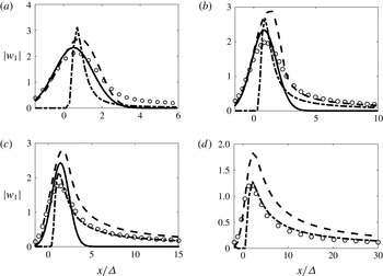
We now consider a more realistic parameter choice relevant to the atmosphere. Taking
 $N=1.4\times 10^{-2}~\text{s}^{-1}$
,
 $f=10^{-4}~\text{s}^{-1}$
,
 $\unicode[STIX]{x1D6EC}=5.6\times 10^{-3}~\text{s}^{-1}$
,
 $H=5~\text{km}$
,
 $\unicode[STIX]{x1D6E5}=3.5\times 10^{2}~\text{km}$
and
 $k_{\ast }=1.43\times 10^{-5}~\text{m}^{-1}$
gives
 $$\begin{eqnarray}\displaystyle Ro=0.4,\quad k_{\ast }\unicode[STIX]{x1D6E5}=5,\quad l_{\ast }\unicode[STIX]{x1D6E5}=5,\quad J=5\quad \text{and}\quad \unicode[STIX]{x1D708}_{\ast }=1, & & \displaystyle\end{eqnarray}$$
so
 $r=k_{\ast }\unicode[STIX]{x1D6E5}Ro=2$
. Since the parameters
 $Ro^{-1}$
,
 $k_{\ast }\unicode[STIX]{x1D6E5}$
and
 $J$
are only moderately large, this choice provides a strict test on the applicability of the asymptotic results. The results for the form of the wavepacket are shown in figure 4. The accuracy of the asymptotic approximations has degraded considerable compared with that in figure 4, unsurprisingly, perhaps, given that the error scales like
 $(k_{\ast }\unicode[STIX]{x1D6E5})^{-1/2}\approx 0.45$
. Nonetheless, there remains a reasonable qualitative match between asymptotic and numerical results which suggests our approximations remain useful.


4 Wave–mean-flow interaction
Section 3 shows that the wave amplitude changes suddenly across the inertial layer. In this section, we exploit our asymptotic expression for the wavepacket structure to derive the mean force exerted in this layer as a result of this change, and to calculate the mean-flow response. The important quantity for this force is the EP flux, which has long been recognised as the relevant diagnostic (Eliassen & Palm Reference Eliassen and Palm1961; Andrews & McIntyre Reference Andrews and McIntyre1976; Boyd Reference Boyd1976; Edmon, Hoskins & McIntyre Reference Edmon, Hoskins and McIntyre1980).
Two types of mean-flow response need to be distinguished: the far-field response, and the local response. The far-field response is the net change in the mean flow that persists far downstream of the mountain; it is a consequence of a change of the horizontally integrated EP flux due to absorption. In contrast, the local response is the mean-flow change caused by local EP flux changes without far-field impact because they integrate to zero horizontally. As discussed in § 3, the net EP flux change is concentrated in the inertial layer where the Regime II
 $_{B}$
approximation applies; below this, the waves are localised horizontally in space and leave no net mean-flow response, in agreement with non-acceleration results. In the remainder of this section, we derive the equation governing mean-flow response (§ 4.1), compute the EP flux divergence that appears as the sole forcing term in this equation (§ 4.2) and compute the mean-flow change asymptotically, taking advantage of the thinness of the inertial layer (§ 4.3).
4.1 Governing equation
Taking advantage of the small Rossby number, the mean flow is calculated using quasi-geostrophic theory. By taking the horizontal curl of the horizontal momentum equation (2.2a
), applying
 $\unicode[STIX]{x2202}_{z}f/N^{2}$
to (2.2c
) and using the incompressibility (2.2d
), we obtain
 $$\begin{eqnarray}\displaystyle & & \displaystyle \unicode[STIX]{x2202}_{t}\left(v_{x}-u_{y}+\unicode[STIX]{x2202}_{z}\left(\frac{f}{N^{2}}b\right)\right)+\underbrace{(\unicode[STIX]{x2202}_{xx}-\unicode[STIX]{x2202}_{yy})(uv)+\unicode[STIX]{x2202}_{xy}(v^{2}-u^{2})}_{(a)}+\underbrace{\unicode[STIX]{x2202}_{z}\left(\frac{f}{N^{2}}\unicode[STIX]{x2202}_{z}(wb)\right)}_{(b)}\nonumber\\ \displaystyle & & \displaystyle \quad +\,\underbrace{\unicode[STIX]{x2202}_{xz}\left(wv+\frac{f}{N^{2}}ub\right)-\unicode[STIX]{x2202}_{yz}\left(wu-\frac{f}{N^{2}}vb\right)}_{(c)}=0.\end{eqnarray}$$
The waves and mean flow are separated by the small-scale average defined as
 $$\begin{eqnarray}\displaystyle \langle \cdot \rangle =\frac{1}{D^{2}}\int _{x}^{x+D}\int _{y}^{y+D}\boldsymbol{\cdot }\,\text{d}\boldsymbol{x}^{\prime }, & & \displaystyle\end{eqnarray}$$
where
 $k_{\ast }^{-1}\ll D\ll \unicode[STIX]{x1D6E5}$
. Because of their small spatial scale, the waves have zero average. Applying this average to (4.1), and using the smallness of the wave amplitude and Rossby number to retain the leading-order terms for both wave and mean flow, we obtain
 $$\begin{eqnarray}\displaystyle (\unicode[STIX]{x2202}_{t}+\unicode[STIX]{x1D6EC}z\unicode[STIX]{x2202}_{x})\left(\unicode[STIX]{x1D6FB}^{\bot }\boldsymbol{\cdot }\boldsymbol{U}+\unicode[STIX]{x2202}_{z}\left(\frac{f}{N^{2}}\langle b_{2}\rangle \right)\right)+\unicode[STIX]{x1D6FB}^{\bot }\boldsymbol{\cdot }\unicode[STIX]{x2202}_{z}\boldsymbol{{\mathcal{F}}}=0, & & \displaystyle\end{eqnarray}$$
where
 $\unicode[STIX]{x1D6FB}^{\bot }=(-\unicode[STIX]{x2202}_{y},\unicode[STIX]{x2202}_{x})$
denotes the horizontal curl, and
 $$\begin{eqnarray}\displaystyle \boldsymbol{{\mathcal{F}}}=\left(\langle u_{1}w_{1}\rangle -\frac{f}{N^{2}}\langle v_{1}b_{1}\rangle ,\langle v_{1}w_{1}\rangle +\frac{f}{N^{2}}\langle u_{1}b_{1}\rangle \right) & & \displaystyle\end{eqnarray}$$
is the vertical part of the EP flux (Eliassen & Palm Reference Eliassen and Palm1961). In (4.3), the mean flow is in geostrophic balance, with
 $$\begin{eqnarray}\displaystyle \langle \boldsymbol{u}_{2}\rangle =(\boldsymbol{U},0)=(U,V,0)=(-\unicode[STIX]{x2202}_{y}\unicode[STIX]{x1D6F9},\unicode[STIX]{x2202}_{x}\unicode[STIX]{x1D6F9},0)\quad \text{and}\quad \langle b_{2}\rangle =f\unicode[STIX]{x2202}_{z}\unicode[STIX]{x1D6F9}, & & \displaystyle\end{eqnarray}$$
where the streamfunction
 $\unicode[STIX]{x1D6F9}$
remains to be determined.
If there is no wave effect,
 $\boldsymbol{{\mathcal{F}}}=0$
, (4.3) reduces to the quasi-geostrophic potential-vorticity (QGPV) equation. Note that term (c) in (4.1) is the only quadratic wave term to contribute to (4.3): term (a) is
 $O(\unicode[STIX]{x1D6FF}_{\ast }/H)$
smaller than term (c) because of the vertically thinness of inertial layer; term (b) has zero average because
 $w_{1}$
and
 $b_{1}$
are out of phase in the limit of large
 $J$
(see (3.14c
)).
The boundary condition associated with (4.3) is obtained by taking the average of (2.3), retaining terms up to second order in the wave amplitude to find
 $$\begin{eqnarray}\displaystyle \langle w_{2}\rangle & = & \displaystyle \langle \boldsymbol{u}_{1}\boldsymbol{\cdot }\unicode[STIX]{x1D735}h_{t}-h_{t}\unicode[STIX]{x2202}_{z}w_{1}-\unicode[STIX]{x1D6EC}h_{t}\unicode[STIX]{x2202}_{x}h_{t}\rangle =\langle \boldsymbol{u}_{1}\boldsymbol{\cdot }\unicode[STIX]{x1D735}h_{t}+h_{t}\unicode[STIX]{x1D735}\boldsymbol{\cdot }\boldsymbol{u}_{1}-\unicode[STIX]{x1D6EC}h_{t}\unicode[STIX]{x2202}_{x}h_{t}\rangle \nonumber\\ \displaystyle & = & \displaystyle \langle \unicode[STIX]{x1D735}\boldsymbol{\cdot }(\boldsymbol{u}_{1}h_{t})-\unicode[STIX]{x1D6EC}\unicode[STIX]{x2202}_{x}(h_{t}^{2}/2)\rangle =0,\end{eqnarray}$$
where
 $\boldsymbol{u}_{1}=(u_{1},v_{1})$
, and the incompressibility condition (3.7d
) is used.
One significant feature of the EP flux is its conservation when the background flow possesses certain symmetries, leading to the non-acceleration theorem (Charney & Drazin Reference Charney and Drazin1961): waves do not force the mean flow unless there exists a singularity or some dissipation. In our set-up, the background shear flow has
 $x$
- and
 $y$
-symmetry, and EP flux conservation is easily demonstrated for a plane wave with wavevector
 $\boldsymbol{k}=(k,l)$
: applying the polarisation relation (3.14) to (4.4), we obtain the plane-wave expression of the EP flux,
 $$\begin{eqnarray}\displaystyle \boldsymbol{{\mathcal{F}}}=(F,\unicode[STIX]{x1D708}F),\quad \text{with }F=\frac{-\unicode[STIX]{x1D6EC}}{f}\frac{1}{1+\unicode[STIX]{x1D708}^{2}}\text{Re}\left(\text{i}\frac{1-\unicode[STIX]{x1D701}^{2}}{\unicode[STIX]{x1D701}^{2}}{\hat{w}}_{\unicode[STIX]{x1D701}}(\boldsymbol{k}){\hat{w}}^{\ast }(\boldsymbol{k})-\unicode[STIX]{x1D708}\frac{{\hat{w}}(\boldsymbol{k}){\hat{w}}^{\ast }(\boldsymbol{k})}{\unicode[STIX]{x1D701}^{2}}\right).\quad & & \displaystyle\end{eqnarray}$$
Its conservation is deduced from (3.11) by multiplication of
 ${\hat{w}}$
by its complex conjugate
 ${\hat{w}}^{\ast }$
and subtraction of the conjugate of the resulting equation to find
 $$\begin{eqnarray}\displaystyle \unicode[STIX]{x2202}_{z}F=0. & & \displaystyle\end{eqnarray}$$
This conservation does not hold across the inertial-level singularities
 $\unicode[STIX]{x1D701}=\pm 1$
. Across the lower one,
 $\unicode[STIX]{x1D701}=1$
, the plane-wave EP flux attenuates to an exponentially small value, leading to the wave forcing of the mean flow in the inertial layer (Regime II
 $_{B}$
). We now compute the EP flux in this layer.
4.2 Eliassen–Palm flux
The derivation of the EP flux is greatly simplified by observing that, in the saddle-point approximations valid in Regimes I and II, the relations of the various wave fields
 $u_{1}$
,
 $v_{1}$
, etc. associated with the wavepacket to
 $w_{1}$
mirror the polarisation relations (3.14). This is because the rapid dependence in
 $x$
of the wave solution corresponds to a plane wave with (possibly complex) wavenumber
 $\boldsymbol{k}_{s}$
given by a saddle-point value of
 $\boldsymbol{k}$
(see appendix A). Using the notation
 $\unicode[STIX]{x1D701}_{s}=-k_{s}\unicode[STIX]{x1D6EC}z/f$
, we obtain
 $$\begin{eqnarray}\displaystyle & \displaystyle u_{1}=\frac{\text{i}(\unicode[STIX]{x1D701}_{s}-\text{i}\unicode[STIX]{x1D708}_{\ast })}{K_{s}\unicode[STIX]{x1D701}_{s}(1+\unicode[STIX]{x1D708}_{\ast }^{2})}w_{1z}-\frac{\text{i}\unicode[STIX]{x1D6EC}\unicode[STIX]{x1D708}_{\ast }^{2}}{f\unicode[STIX]{x1D701}_{s}(1+\unicode[STIX]{x1D708}_{\ast }^{2})}w_{1}, & \displaystyle\end{eqnarray}$$
 $$\begin{eqnarray}\displaystyle & \displaystyle v_{1}=-\frac{1-\text{i}\unicode[STIX]{x1D708}_{\ast }\unicode[STIX]{x1D701}_{s}}{K_{s}\unicode[STIX]{x1D701}_{s}(1+\unicode[STIX]{x1D708}_{\ast }^{2})}w_{1z}+\frac{\text{i}\unicode[STIX]{x1D6EC}\unicode[STIX]{x1D708}_{\ast }}{f\unicode[STIX]{x1D701}_{s}(1+\unicode[STIX]{x1D708}_{\ast }^{2})}w_{1}, & \displaystyle\end{eqnarray}$$
 $$\begin{eqnarray}\displaystyle & \displaystyle b_{1}=-\frac{\text{i}\unicode[STIX]{x1D6EC}(1-\text{i}\unicode[STIX]{x1D708}_{\ast }\unicode[STIX]{x1D701}_{s})}{K_{s}\unicode[STIX]{x1D701}_{s}^{2}(1+\unicode[STIX]{x1D708}_{\ast }^{2})}w_{1z}+\text{i}\frac{\unicode[STIX]{x1D6EC}^{2}}{f}\left(\frac{\text{i}\unicode[STIX]{x1D708}_{\ast }}{\unicode[STIX]{x1D701}_{s}^{2}(1+\unicode[STIX]{x1D708}_{\ast }^{2})}+\frac{J^{2}}{\unicode[STIX]{x1D701}_{s}}\right)w_{1}, & \displaystyle\end{eqnarray}$$
 $\unicode[STIX]{x1D708}_{s}=l_{s}/k_{s}\sim l_{\ast }/k_{\ast }=\unicode[STIX]{x1D708}_{\ast }$
to leading order. Correspondingly, a derivation that parallels that of (4.7) gives the
 $x$
-component of the wavepacket EP flux as
 $$\begin{eqnarray}\displaystyle F=\frac{1}{1+\unicode[STIX]{x1D708}_{\ast }^{2}}\text{Re}\left(\frac{\text{i}}{k_{s}}\frac{1-\unicode[STIX]{x1D701}_{s}^{2}}{\unicode[STIX]{x1D701}_{s}^{2}}w_{1z}w_{1}^{\ast }-\unicode[STIX]{x1D708}_{\ast }\frac{w_{1}w_{1}^{\ast }}{\unicode[STIX]{x1D701}_{s}^{2}}\right). & & \displaystyle\end{eqnarray}$$
This can be simplified further. Focussing on Regime II
 $_{B}$
, we observe that the
 $O(\unicode[STIX]{x1D716})$
vertical scale implies that the first term in the brackets in (4.10) dominates the second, that
 $k_{s}$
can be approximated by
 $k_{\ast }$
, and that
 $\unicode[STIX]{x1D701}_{s}$
can be approximated by
 $1$
except in the factor
 $1-\unicode[STIX]{x1D701}_{s}$
of
 $1-\unicode[STIX]{x1D701}_{s}^{2}$
. This leads to the simple expression
 $$\begin{eqnarray}\displaystyle F=\frac{2(1-\unicode[STIX]{x1D701}_{s})}{k_{\ast }(1+\unicode[STIX]{x1D708}_{\ast }^{2})}\text{Re}\left(\text{i}w_{1z}w_{1}^{\ast }\right). & & \displaystyle\end{eqnarray}$$
Now, using that
 $\unicode[STIX]{x2202}_{z}=-k^{\ast }\unicode[STIX]{x1D6E5}\unicode[STIX]{x1D6EC}\unicode[STIX]{x2202}_{Z}/f$
, we obtain from the form of
 $w_{1}$
in (A 15) that, to leading order,
 $$\begin{eqnarray}\displaystyle w_{1z}\sim \frac{\text{i}(k_{\ast }\unicode[STIX]{x1D6FF})^{3/2}k_{\ast }\unicode[STIX]{x1D6EC}}{f}w_{1}. & & \displaystyle\end{eqnarray}$$
Introducing this result into (4.11) and using that
 $$\begin{eqnarray}\displaystyle \unicode[STIX]{x1D701}_{s}=1+\frac{1}{k_{\ast }\unicode[STIX]{x1D6E5}}(K_{s}+Z), & & \displaystyle\end{eqnarray}$$
together with the explicit form (A 14) of
 $K_{s}$
, we find that
 $$\begin{eqnarray}\displaystyle F=\frac{J^{2}\unicode[STIX]{x1D6EC}}{(k_{\ast }\unicode[STIX]{x1D6E5})^{3/2}fX}|w_{1}|^{2}. & & \displaystyle\end{eqnarray}$$
The explicit form of
 $w_{1}$
in (3.42) can finally be used to obtain the explicit expression
 $$\begin{eqnarray}\displaystyle F=\frac{E}{X^{3}}\text{e}^{-(a^{2}/X^{2}-Z)^{2}}g^{2}(y), & & \displaystyle\end{eqnarray}$$
where
 $$\begin{eqnarray}\displaystyle E=\frac{J^{3}\unicode[STIX]{x1D6EC}h^{2}f(r^{2}-1)^{1/2}(1+\unicode[STIX]{x1D708}_{\ast }^{2})^{1/2}}{(k_{\ast }\unicode[STIX]{x1D6E5})^{5/2}} & & \displaystyle\end{eqnarray}$$
is a constant controlling the amplitude of
 $F$
. This expression only holds for
 $X>0$
; for
 $X<0$
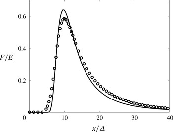
, the EP flux is exponentially small. We emphasise the remarkably simple form of (4.15): notwithstanding the many parameters involved, the formula is well suited for practical use in parameterisations.
We illustrate the form of the EP flux in figure 5 by showing its contours in the
 $(x,z)$
cross-section where it is maximised, using the parameters in (3.46). The EP flux is computed from the WKB linear solution (3.20) and polarisation relation (3.14). The validity of the asymptotic approximation is confirmed by figure 6 which compares the EP flux obtained numerically with the asymptotic approximation at the dominant inertial level.
Contours of the EP flux in (4.15) normalised by the largest value at the bottom
 $(3/4)^{3/4}\text{e}^{-3/4}E$
for the parameters in (3.46); 7 equispaced contours in the range
 $[0.125,0.875]$
are shown in the main figure, and in the inset, 9 equispaced contours are in the range
 $[0.03,0.27]$
. The contours can be compared with those of the vertical velocity
 $|w_{1}|$
shown in figure 2: although the two fields obey the same scaling, the maximum of the EP flux is closer to the mountain. The inset zooms on the rectangular box indicated in the main panel.

EP flux at the dominant inertial level for the parameters in (3.46): numerical results (circles) are compared with the prediction of the Regime II
 $_{B}$
approximation (solid line).

By integrating (4.15) over
 $x$
and
 $y$
, we obtain the horizontally integrated EP flux
 $$\begin{eqnarray}\displaystyle \overline{F}=\frac{\unicode[STIX]{x03C0}J\unicode[STIX]{x1D6E5}^{2}\unicode[STIX]{x1D6EC}h^{2}f(r^{2}-1)^{1/2}}{2(1+\unicode[STIX]{x1D708}_{\ast }^{2})^{1/2}}(1+\text{erf}Z), & & \displaystyle\end{eqnarray}$$
where the decay of the error function to
 $0$
as
 $Z\rightarrow -\infty$
(above the inertial layer) clearly captures wave absorption. As
 $Z\rightarrow \infty$
, i.e. well below the dominant inertial level,
 $\overline{F}$
tends to the constant value
 $$\begin{eqnarray}\displaystyle \overline{F}_{tot}=\frac{\unicode[STIX]{x03C0}J\unicode[STIX]{x1D6E5}^{2}\unicode[STIX]{x1D6EC}h^{2}f(r^{2}-1)^{1/2}}{(1+\unicode[STIX]{x1D708}_{\ast }^{2})^{1/2}}. & & \displaystyle\end{eqnarray}$$
This matches the horizontally integrated EP flux at the ground, since the flux is conserved below the inertial layer. We check this in appendix B. We note that
 $\overline{F}_{tot}$
is finite in the limit
 $f\rightarrow 0$
, where it is given by
 $\overline{F}_{tot}=\unicode[STIX]{x03C0}N\unicode[STIX]{x1D6EC}\unicode[STIX]{x1D6E5}^{2}h^{2}k_{\ast }H$
. The integrated EP flux
 $\overline{F}$
becomes discontinuous in this limit, jumping from
 $\overline{F}_{tot}$
to
 $0$
across the critical level.
From (4.17), we can also estimate the wave drag per unit area, defined as the vertical derivative of horizontally integrated EP flux divided by
 $\unicode[STIX]{x1D6E5}^{2}$
:
 $$\begin{eqnarray}\displaystyle \overline{f(Z)}=\frac{\unicode[STIX]{x2202}_{z}\overline{F(Z)}}{\unicode[STIX]{x1D6E5}^{2}}=-\frac{\sqrt{\unicode[STIX]{x03C0}}}{2}\unicode[STIX]{x1D6EC}N\unicode[STIX]{x0394}h^{2}k_{\ast }^{2}\frac{k_{\ast }}{|\boldsymbol{k}_{\ast }|}(r^{2}-1)^{1/2}\text{e}^{-Z^{2}}, & & \displaystyle\end{eqnarray}$$
where
 $|\boldsymbol{k}_{\ast }|=\sqrt{k_{\ast }^{2}+l_{\ast }^{2}}$
is the amplitude of the dominant wavenumber.
4.3 Mean-flow response
We now consider the mean-flow response to the wave drag associated with the
 $z$
-dependent EP flux (4.15). We compute the steady flow response by solving the QGPV equation (4.3) asymptotically, taking advantage of the thinness of the inertial layer where the wave drag acts to apply matched asymptotics. Thus the domain
 $z>-H$
is separated into an inner region around the inertial level
 $z\approx z_{\ast }$
, specifically
 $Z=-k_{\ast }^{2}\unicode[STIX]{x1D6E5}\unicode[STIX]{x1D6EC}(z-z_{\ast })/f=O(1)$
, and an outer region where the wave drag is absent. Simplifications arise because the spatial scale in the
 $x$
-direction is longer than in the
 $y$
-direction; this is made explicit using the variable
 $X$
defined in (A 16), with
 $X=O(1)$
implying that
 $x=\unicode[STIX]{x1D6E5}\times O((k_{\ast }\unicode[STIX]{x1D6E5})^{1/2})$
We denote the streamfunction associated with the wave-induced mean flow in the inner and outer regions by
 $\unicode[STIX]{x1D6F9}(X,y,Z)$
and
 $\unicode[STIX]{x1D713}(X,y,z)$
, respectively. In the inner region, considering the scalings of Regime II
 $_{B}$
, the steady (
 $\unicode[STIX]{x2202}_{t}=0$
) QGPV equation (4.3) becomes
 $$\begin{eqnarray}\displaystyle & & \displaystyle \unicode[STIX]{x1D716}^{1/2}k_{\ast }(k_{\ast }\unicode[STIX]{x1D6E5})^{-3/2}(U_{\ast }\unicode[STIX]{x2202}_{X}+\unicode[STIX]{x1D6FB}^{\bot }\unicode[STIX]{x1D6F9}\boldsymbol{\cdot }\unicode[STIX]{x1D735})\left(\unicode[STIX]{x1D716}k_{\ast }^{2}(k_{\ast }\unicode[STIX]{x1D6E5})^{-3}\unicode[STIX]{x2202}_{XX}\unicode[STIX]{x1D6F9}+\unicode[STIX]{x2202}_{yy}\unicode[STIX]{x1D6F9}+\frac{k_{\ast }^{4}\unicode[STIX]{x1D6E5}^{2}}{\unicode[STIX]{x1D716}^{2}J^{2}}\unicode[STIX]{x2202}_{ZZ}\unicode[STIX]{x1D6F9}\right)\nonumber\\ \displaystyle & & \displaystyle \qquad =\frac{k_{\ast }^{2}\unicode[STIX]{x1D6EC}\unicode[STIX]{x1D6E5}}{\unicode[STIX]{x1D716}^{2}f}\unicode[STIX]{x2202}_{yZ}F,\end{eqnarray}$$
where
 $\unicode[STIX]{x1D735}$
and
 $\unicode[STIX]{x1D6FB}^{\bot }$
are gradients with respect to the scaled variables
 $(X,y)$
,
 $U_{\ast }=-\unicode[STIX]{x1D6EC}z_{\ast }=f/k_{\ast }$
is the background velocity at the dominant inertial level, and we have included the bookkeeping parameter
 $\unicode[STIX]{x1D716}$
. On the right-hand side we have neglected the
 $x$
derivative of
 $\unicode[STIX]{x2202}_{z}F$
against the
 $y$
-derivative, owing to the asymptotically larger scales in
 $x$
.
For sufficiently small mountain height, equation (4.20) can be linearised; we make explicit below the condition for this approximation to hold. Retaining only the leading-order terms in (4.20) reduces this to
 $$\begin{eqnarray}\displaystyle \frac{k_{\ast }^{3}(k_{\ast }\unicode[STIX]{x1D6E5})^{1/2}}{\unicode[STIX]{x1D716}^{3/2}J^{2}}U_{\ast }\unicode[STIX]{x2202}_{XZZ}\unicode[STIX]{x1D6F9}=\frac{k_{\ast }^{2}\unicode[STIX]{x1D6EC}\unicode[STIX]{x1D6E5}}{\unicode[STIX]{x1D716}^{2}f}\unicode[STIX]{x2202}_{yZ}F. & & \displaystyle\end{eqnarray}$$
Since
 $F$
is exponentially small for
 $X<0$
, we can integrate (4.21) for
 $X>0$
to obtain
 $$\begin{eqnarray}\displaystyle \unicode[STIX]{x2202}_{ZZ}\unicode[STIX]{x1D6F9}=Q, & & \displaystyle\end{eqnarray}$$
where
 $$\begin{eqnarray}\displaystyle Q=Q(X,y,Z)=\frac{J^{2}\unicode[STIX]{x1D6EC}(k_{\ast }\unicode[STIX]{x1D6E5})^{1/2}}{\unicode[STIX]{x1D716}^{1/2}U_{\ast }k_{\ast }^{2}f}\int _{0}^{X}\unicode[STIX]{x2202}_{yZ}F(X^{\prime },y,Z)\,\text{d}X^{\prime } & & \displaystyle\end{eqnarray}$$
can be interpreted as a scaled wave-induced QGPV. This can be computed explicitly using (4.15) to find
 $$\begin{eqnarray}\displaystyle Q=\frac{J^{3}\unicode[STIX]{x1D6EC}^{2}\unicode[STIX]{x0394}h^{2}(r^{2}-1)^{1/2}}{f(k_{\ast }\unicode[STIX]{x1D6E5})(1+\unicode[STIX]{x1D708}_{\ast }^{2})^{1/2}}\,\text{e}^{-(a^{2}/X^{2}-Z)^{2}}\unicode[STIX]{x2202}_{y}g^{2}, & & \displaystyle\end{eqnarray}$$
with
 $g(y)$
defined in (3.37).
Equation (4.22) is readily integrated, leading to
 $$\begin{eqnarray}\displaystyle \unicode[STIX]{x1D6F9}(X,y,Z)=\int _{0}^{Z}\int _{0}^{Z^{\prime }}Q(x,Y,Z^{\prime \prime })\,\text{d}Z^{\prime }\,\text{d}Z^{\prime \prime }+C_{1}(X,y)Z+\unicode[STIX]{x1D716}^{-1}C_{2}(X,y), & & \displaystyle\end{eqnarray}$$
where
 $C_{1}$
and
 $C_{2}$
are integration ‘constants’ that are determined by matching the outer solution (cf. Plougonven & Vanneste Reference Plougonven and Vanneste2010). We have anticipated that the
 $Z$
-independent term is an order
 $\unicode[STIX]{x1D716}^{-1}$
larger than the other terms. Matching requires the asymptotic behaviour of
 $\unicode[STIX]{x1D6F9}$
as
 $Z\rightarrow \pm \infty$
, found to be
 $$\begin{eqnarray}\displaystyle \unicode[STIX]{x1D6F9}(X,y,Z) & {\sim} & \displaystyle Z\left(\int _{0}^{\pm \infty }Q(X,y,Z^{\prime })\,\text{d}Z^{\prime }+C_{1}(X,y)\right)+\unicode[STIX]{x1D716}^{-1}C_{2}(X,y)\nonumber\\ \displaystyle & & \displaystyle -\,\int _{0}^{\pm \infty }Z^{\prime }Q(X,y,Z^{\prime })\,\text{d}Z^{\prime }\end{eqnarray}$$
as
 $Z\rightarrow \pm \infty$
.
In the outer region, the QGPV equation (4.3) is
 $$\begin{eqnarray}\displaystyle \unicode[STIX]{x1D6EC}z\unicode[STIX]{x2202}_{X}\left(\unicode[STIX]{x2202}_{yy}\unicode[STIX]{x1D713}+\unicode[STIX]{x1D716}k_{\ast }^{2}(k_{\ast }\unicode[STIX]{x1D6E5})^{-3}\unicode[STIX]{x2202}_{XX}\unicode[STIX]{x1D713}+\frac{f^{2}}{N^{2}}\unicode[STIX]{x2202}_{zz}\unicode[STIX]{x1D713}\right)=0, & & \displaystyle\end{eqnarray}$$
which, to the leading order, reduces to
 $$\begin{eqnarray}\displaystyle \unicode[STIX]{x1D6EC}z\unicode[STIX]{x2202}_{X}\left(\unicode[STIX]{x2202}_{yy}\unicode[STIX]{x1D713}+\frac{f^{2}}{N^{2}}\unicode[STIX]{x2202}_{zz}\unicode[STIX]{x1D713}\right)=0. & & \displaystyle\end{eqnarray}$$
Integrating in
 $X$
, we find that
 $$\begin{eqnarray}\displaystyle \unicode[STIX]{x2202}_{yy}\unicode[STIX]{x1D713}+\frac{f^{2}}{N^{2}}\unicode[STIX]{x2202}_{zz}\unicode[STIX]{x1D713}=0. & & \displaystyle\end{eqnarray}$$
This is best solved using a Fourier transform in the
 $y$
direction. Denoting this transform by a hat, we have
 $$\begin{eqnarray}\displaystyle \hat{\unicode[STIX]{x1D713}}=\left\{\begin{array}{@{}ll@{}}\displaystyle \unicode[STIX]{x1D716}^{-1}{\hat{C}}_{3}(X,l)\text{e}^{-N|l|(z-z_{\ast })/f}\quad & \text{for }z>z_{\ast }\\ \displaystyle \unicode[STIX]{x1D716}^{-1}{\hat{C}}_{4}(X,l)\text{e}^{-N|l|(z-z_{\ast })/f}+\unicode[STIX]{x1D716}^{-1}{\hat{C}}_{5}(X,l)\text{e}^{N|l|(z-z_{\ast })/f}\quad & \text{for }z<z_{\ast },\end{array}\right. & & \displaystyle\end{eqnarray}$$
applying a vanishing boundary condition as
 $z\rightarrow \infty$
. Combining the condition (4.6) of zero mean vertical velocity with the buoyancy equation
 $U\unicode[STIX]{x2202}_{X}\unicode[STIX]{x1D713}_{z}=0$
stemming from (2.2c
), we find the condition
 $\unicode[STIX]{x1D713}_{z}=0$
at the lower boundary
 $z=-H$
. This implies
 $$\begin{eqnarray}\displaystyle {\hat{C}}_{4}\text{e}^{N|l|(H+z_{\ast })/f}={\hat{C}}_{5}\text{e}^{-N|l|(H+z_{\ast })/f}. & & \displaystyle\end{eqnarray}$$
We now match (4.30) to (4.26) to determine
 ${\hat{C}}_{3}$
,
 ${\hat{C}}_{4}$
and
 ${\hat{C}}_{5}$
, and hence the outer solution, completely. Substituting
 $z-z_{\ast }=-\unicode[STIX]{x1D716}fZ/(k_{\ast }^{2}\unicode[STIX]{x0394}\unicode[STIX]{x1D6EC})$
into (4.30), expanding in powers of
 $\unicode[STIX]{x1D716}$
and matching with (4.26), we find that
 $$\begin{eqnarray}\displaystyle {\hat{C}}_{4}+{\hat{C}}_{5}={\hat{C}}_{3}\,(={\hat{C}}_{2}), & & \displaystyle\end{eqnarray}$$
and
 $$\begin{eqnarray}\displaystyle {\hat{C}}_{4}-{\hat{C}}_{5}-{\hat{C}}_{3} & = & \displaystyle \frac{k_{\ast }^{2}\unicode[STIX]{x1D6E5}}{J|l|}\int _{-\infty }^{\infty }\hat{Q}(X,l,Z^{\prime })\,\text{d}Z^{\prime }\nonumber\\ \displaystyle & = & \displaystyle \frac{\sqrt{\unicode[STIX]{x03C0}}J^{2}(k_{\ast }\unicode[STIX]{x1D6E5})\unicode[STIX]{x1D6EC}^{2}h^{2}(r^{2}-1)^{1/2}}{f(1+\unicode[STIX]{x1D708}_{\ast }^{2})^{1/2}}\frac{\widehat{\unicode[STIX]{x2202}_{y}g^{2}}}{|l|}.\end{eqnarray}$$
Thus, (4.31), (4.32) and (4.33) provide three equations for
 ${\hat{C}}_{3}$
,
 ${\hat{C}}_{4}$
and
 ${\hat{C}}_{5}$
and hence determine the mean flow. The solution to these equations is straightforward but leads to lengthy expressions which we relegate to appendix C.
Remarkably, the right-hand side of (4.33) and hence
 ${\hat{C}}_{3}$
,
 ${\hat{C}}_{4}$
and
 ${\hat{C}}_{5}$
do not depend on
 $X$
. As a result,
 $\unicode[STIX]{x1D713}$
,
 $\unicode[STIX]{x1D6F9}$
and thus the entire mean-flow response does not change downstream of the mountain. Our solution suggests that there is a jump in this response, from a zero value for
 $X<0$
to the
 $X$
-independent value for
 $X>0$
. This is an artefact of the asymptotic approximation: the transition to a non-zero mean flow is in fact smooth. Its detailed form could be obtained using the approximation of the wave fields in Regime II. Here we only note that the scaling of Regime II indicates that the transition region has a characteristic length
 $x/\unicode[STIX]{x1D6E5}=O((k_{\ast }\unicode[STIX]{x1D6E5})^{1/3})$
, asymptotically smaller than the
 $O((k_{\ast }\unicode[STIX]{x1D6E5})^{1/2})$
scale that is resolved by the Regime IIB approximation used in our computation of the mean-flow response, hence the apparent discontinuity.
Equation (4.33) provides an estimate for the order of magnitude of the mean-flow response. Recalling that the change in mean velocity is
 $-\unicode[STIX]{x2202}_{y}\unicode[STIX]{x1D713}$
with the
 $y$
-scale
 $\unicode[STIX]{x1D6E5}$
, and noting that the maximum value of
 $\unicode[STIX]{x1D713}$
is
 $O({\hat{C}}_{3})$
, we estimate the wave-induced mean velocity as
 $$\begin{eqnarray}\displaystyle U_{w}=O\left(J^{2}r\left(\frac{h}{H}\right)^{2}U_{b}\right), & & \displaystyle\end{eqnarray}$$
assuming that
 $(r^{2}-1)^{1/2}=O(1)$
. Since
 $(k_{\ast }\unicode[STIX]{x1D6E5})Ro=O(1)$
, this indicates that
 $U_{w}\ll U_{b}$
, as required for the linearisation of the QGPV equation, provided that
 $J(h/H)\ll 1$
.
Mean-flow response. (a) Contours of the wave-induced mean flow
 $\langle u_{2}\rangle$
, with the sign indicated by
 $\pm$
; 20 equispaced contours in the range
 $[-0.52,0.13]$
are shown. (b)
 $\langle u_{2}\rangle$
at
 $z/H=-0.9,-0.5,0$
, with
 $z=-0.5$
corresponding to the dominant inertial level. The mean flow is normalised by
 $\sqrt{3\unicode[STIX]{x03C0}}k_{\ast }J^{2}\unicode[STIX]{x1D6EC}^{2}h^{2}/f$
. (c) Mean pressure
 $\langle \unicode[STIX]{x1D719}_{2}\rangle$
at ground level (
 $z=-H$
), normalised by
 $\sqrt{3\unicode[STIX]{x03C0}}k_{\ast }\unicode[STIX]{x0394}J^{2}\unicode[STIX]{x1D6EC}^{2}h^{2}$
.

To illustrate our results, we have calculated the mean-flow response for
 $J=k_{\ast }\unicode[STIX]{x1D6E5}$
,
 $l_{\ast }=0$
and
 $r=2$
. The linear system (4.31), (4.32) and (4.33) is readily solved for
 ${\hat{C}}_{3}$
,
 ${\hat{C}}_{4}$
and
 ${\hat{C}}_{5}$
, leading to
 $\hat{\unicode[STIX]{x1D713}}$
and, after Fourier inversion, to the mean flow
 $\langle u_{2}\rangle =-\unicode[STIX]{x2202}_{y}\unicode[STIX]{x1D713}$
and mean pressure
 $\langle \unicode[STIX]{x1D719}_{2}\rangle$
. This is displayed in figure 7. Observe that the mean-flow response to the wave drag localised in the thin inertial layer is distributed through the entire depth of the fluid, and that the total mean-flow change
 $\int \langle u_{2}\rangle \,\text{d}y$
vanishes at each altitude since the streamfunction
 $\unicode[STIX]{x1D713}$
vanishes as
 $y\rightarrow \pm \infty$
.
In the limit of
 $f\rightarrow 0$
, i.e.
 $r\rightarrow \infty$
, (4.33) indicates that
 $U_{w}\rightarrow \infty$
. This is because the quasi-geostrophic approximation breaks down: the wave forcing associated with the jump in the EP flux cannot be balanced by the Coriolis force but instead leads to an acceleration of the mean flow. A more meaningful limit treats
 $f$
as finite for the mean-flow response but sets it to
 $0$
for the evaluation of the EP flux. The fact, noted in § 3.2, that the EP flux undergoes a discontinuous jump in this case has little impact on the mean-flow response since, with the QGPV equation (4.3) remaining valid, the mean flow away from the inertial layer depends only on the magnitude of the jump and not on the details of its structure. Note however that the right-hand side of (4.34) needs to multiplied by an extra factor
 $r$
to account for the fact that
 $(r^{2}-1)^{1/2}\sim r\gg 1$
.
5 Conclusion
In this paper, we study the propagation of a mountain IGW wavepacket in a rotating shear flow and the mean flow generated as a result of wave absorption at inertial-level singularities. The broad wavenumber spectrum of the wavepacket and the dependence of the inertial-level altitude on wavenumber lead to a smearing out of the singularities over a finite-thickness inertial layer where the mean-flow forcing concentrates. Thus, in contrast with the situation when rotation is neglected, dissipative processes can be neglected completely (except in determining branches at singularities) in the computation of the wavepacket and mean-flow response.
Scaling regimes for the mountain wavepacket: the wavepacket is generated by a backsheared flow over a two-scale topography, with a scale separation characterised by
 $k_{\ast }\unicode[STIX]{x1D6E5}\ll 1$
. Two distinguished regimes are found: Regime I and Regime II corresponding to distances from the dominant inertial level that are
 $O(H)$
and
 $O((k_{\ast }\unicode[STIX]{x1D6E5})^{-2/3}H)$
, respectively. The wave drag is localised in a region described by the limiting Regime II
 $_{B}$
, of
 $O(\unicode[STIX]{x1D6E5}_{\ast })$
thickness around the dominant inertial level. This region is located a large,
 $O((k_{\ast }\unicode[STIX]{x1D6E5})^{1/2}\unicode[STIX]{x1D6E5})$
distance downstream of the mountain and extending horizontally over an
 $O((k_{\ast }\unicode[STIX]{x1D6E5})^{1/2}\unicode[STIX]{x1D6E5})$
scale.

By applying a steepest-descent method, we obtain explicit approximations for the form of the wavepacket in different regions characterised by their distance to the dominant inertial level, that is, the inertial level corresponding to the central wavenumber of the mountain profile. Our main conclusions concern the scaling of the wave solution and mean-flow forcing; they are indicated in figure 8. In Regime I, the wavepacket is sufficiently far away from the dominant inertial level that singular effects are not important. Standard ray-tracing results apply: the wavepacket resembles the topography, with envelope scale
 $\unicode[STIX]{x1D6E5}$
. In Regime II the wavepacket is close to the dominant inertial level and hence strongly affected by the inertial-level singularity in the vertical structure (3.23) corresponding to a single wavenumber. As a consequence, ray tracing does not apply, and the wavepacket has a characteristic streamwise scale
 $(k_{\ast }\unicode[STIX]{x1D6E5})^{1/3}\unicode[STIX]{x1D6E5}$
, much longer than the scale of the topography. In Regime II
 $_{B}$
, a subregime of Regime II, the wavepacket is closer still to the dominant inertial level and is absorbed. We pay special attention to this regime since it is relevant to the region where the horizontally integrated EP flux varies vertically, leading to a drag on the mean flow. Qualitatively, our most important conclusion is about the location of this region, found to be an
 $O((k_{\ast }\unicode[STIX]{x1D6E5})^{1/2}\unicode[STIX]{x1D6E5})$
distance downstream of the mountain and to have an
 $O((k_{\ast }\unicode[STIX]{x1D6E5})^{1/2}\unicode[STIX]{x1D6E5})$
horizontal extent. Since
 $k_{\ast }\unicode[STIX]{x1D6E5}\gg 1$
, this makes it evident that mountain waves exert their drag far downstream of the mountain. This is in sharp contrast with their parameterisations in atmospheric models which are typically columnar, assuming that wave propagation is purely vertical and imposing their wave drag right above the wave source (see Hasha, Bühler & Scinocca Reference Hasha, Bühler and Scinocca2008, however).
Using the form of the wave solution in Regime II
 $_{B}$
, we compute the far-field mean-flow response, taking advantage of the smallness of the Rossby number to use a quasi-geostrophic approximation. The vertical divergence of the EP flux, which controls the mean-flow response in this approximation, is localised in the thin inertial layer, with vertical scale
 $\unicode[STIX]{x1D6FF}_{\ast }$
defined in (3.16). The mean-flow response itself, however, has a large scale in both the horizontal and vertical directions because of the non-locality in the diagnostic relation between the mean potential vorticity and mean streamfunction in the quasi-geostrophic approximation.
An interesting feature of the mean-flow generation predicted by the Regime II
 $_{B}$
approximation is that it is zero in the region with
 $X=k_{\ast }^{-1/2}\unicode[STIX]{x1D6E5}^{-3/2}x<0$
but jumps to an
 $X$
-independent value for
 $X\geqslant 0$
. Implicit to this prediction is an assumption that
 $X=O(1)$
, which gives the characteristic horizontal scale of the wavepacket in the inertial layer. The mean flow is in fact smoothly switched on over a shorter characteristic scale, specifically,
 $x/\unicode[STIX]{x1D6E5}=O((k_{\ast }\unicode[STIX]{x1D6E5})^{1/3})$
. This result can be obtained using the Regime II approximations, but we do not carry out detailed calculations which are complicated by the presence of a branch cut in (3.36).
We emphasise that our results are more general than might seem at first glance. Our derivations are based on the distinguished scaling
 $Ro=O((k_{\ast }\unicode[STIX]{x1D6E5})^{-1})$
,
 $J=O(k_{\ast }\unicode[STIX]{x1D6E5})$
, with
 $k_{\ast }\unicode[STIX]{x1D6E5}\gg 1$
, and
 $Jh/H\ll 1$
. In fact, their validity only requires that
 $$\begin{eqnarray}\displaystyle J\frac{h}{H}\ll 1,\quad k_{\ast }\unicode[STIX]{x1D6E5}\gg 1,\quad J\gg 1,\quad Ro\ll 1\quad \text{and}\quad r>1, & & \displaystyle\end{eqnarray}$$
corresponding to the validity of the hypotheses of (i) linear wave, (ii) scale separation of the mountain height, (iii) WKB scaling as in Lott et al. (Reference Lott, Plougonven and Vanneste2012), (iv) quasi-geostrophic mean flow and (v) the dominant inertial level located above ground, ensuring that the argument of the square root in (4.19) is positive. If the conditions in (5.1) are satisfied but the scaling differs from the assumed distinguished scaling, e.g. because
 $J\gg k_{\ast }\unicode[STIX]{x1D6E5}$
, our results continue to hold and could in fact be simplified by taking into account the existence of additional small parameters, such as
 $\unicode[STIX]{x0394}k_{\ast }/J$
in our example.
We conclude by assessing the validity of the assumption of infinitesimally small viscosity, which leads to a vertical scale of wave absorption given by the inertial-layer thickness (3.16). For a finite viscosity, the viscous vertical scale
 $\unicode[STIX]{x1D6FF}_{d}=(\unicode[STIX]{x1D708}N^{2}/k_{\ast })^{1/3}/\unicode[STIX]{x1D6EC}$
is found by considering the Taylor–Goldstein equation with dissipation,
 $D_{t}^{2}\unicode[STIX]{x1D6FB}^{2}w+N^{2}w_{xx}=\unicode[STIX]{x1D708}D_{t}\unicode[STIX]{x1D6FB}^{4}w$
, with
 $D_{t}=\unicode[STIX]{x1D6EC}z\unicode[STIX]{x2202}_{x}$
. The ratio
 $\unicode[STIX]{x1D6FF}_{d}/\unicode[STIX]{x1D6FF}_{\ast }$
which measures the relative strength of viscosity and rotation in setting up the wave vertical scale is then found as
 $\unicode[STIX]{x1D6FF}_{d}/\unicode[STIX]{x1D6FF}_{\ast }=\unicode[STIX]{x0394}k_{\ast }^{5/3}(\unicode[STIX]{x1D708}N^{2})^{1/3}/f$
, independent of the shear
 $\unicode[STIX]{x1D6EC}$
and relatively insensitive to the value of
 $\unicode[STIX]{x1D708}$
. Taking the atmospheric values
 $\unicode[STIX]{x1D708}=10^{-8}~\text{m}^{2}~\text{s}^{-1}$
,
 $N=10^{-2}~\text{s}^{-1}$
,
 $f=10^{-4}~\text{s}^{-1}$
,
 $k=10^{-3}~\text{m}^{-1}$
and
 $\unicode[STIX]{x1D6E5}=10^{4}~\text{m}$
as an illustration, we compute
 $\unicode[STIX]{x1D6FF}_{d}/\unicode[STIX]{x1D6FF}_{\ast }=10^{-1}$
, indicating a dominance of the rotation effects considered in this paper.
Acknowledgements
This research is funded by the UK Natural Environment Research Council (grant NE/J022012/1). J.-H.X. acknowledges financial support from the Centre for Numerical Algorithms and Intelligent Software (NAIS).
Appendix A. Details of wave solution
In this appendix we provide details of the derivation of the saddle-point approximations to the wavepacket in § 3.
A.1 Regime I
In this section we consider altitudes well below the inertial level, corresponding to the scaling (3.29) for
 $z$
with
 $\unicode[STIX]{x1D6FC}=0$
, that is, to
 $$\begin{eqnarray}\displaystyle \unicode[STIX]{x1D701}_{\ast }=-\frac{k_{\ast }\unicode[STIX]{x1D6EC}z}{f}=1+Z_{I},\quad \text{with }Z_{I}=O(1). & & \displaystyle\end{eqnarray}$$
As discussed in § 3.2, the associated distinguished regime is obtained by considering the scaling (3.30) for the wavenumber
 $k$
. Substituting (3.30) and (A 1) into (3.27), we obtain
 $$\begin{eqnarray}\displaystyle w_{1} & = & \displaystyle \frac{\text{i}U_{b}hk_{\ast }\unicode[STIX]{x1D6E5}}{\unicode[STIX]{x1D716}\sqrt{2\unicode[STIX]{x03C0}}}\frac{k_{\ast }}{\unicode[STIX]{x1D716}}\left(\frac{\unicode[STIX]{x1D716}}{k_{\ast }\unicode[STIX]{x1D6E5}}\right)^{\unicode[STIX]{x1D6FD}}\exp (-(y-J\unicode[STIX]{x1D708}_{\ast }k_{\ast }^{-1}(1+\unicode[STIX]{x1D708}_{\ast }^{2})^{-1/2}D_{I})^{2}/(2\unicode[STIX]{x1D6E5}^{2}))\nonumber\\ \displaystyle & & \displaystyle \times \,\int _{-\infty }^{\infty }\frac{(1+Z_{I})}{r}\left(\frac{r^{2}-1}{2Z_{I}+Z_{I}^{2}}\right)^{1/4}\exp (-\unicode[STIX]{x1D716}^{2\unicode[STIX]{x1D6FD}-2}(k_{\ast }\unicode[STIX]{x1D6E5})^{2-2\unicode[STIX]{x1D6FD}}K_{I}^{2}/2\nonumber\\ \displaystyle & & \displaystyle +\,\text{i}\unicode[STIX]{x1D716}^{\unicode[STIX]{x1D6FD}-1}k_{\ast }(k_{\ast }\unicode[STIX]{x1D6E5})^{-\unicode[STIX]{x1D6FD}}K(x-X_{cI})\!)\,\text{d}K_{I},\end{eqnarray}$$
where
 $$\begin{eqnarray}\displaystyle X_{cI}=\frac{J}{k_{\ast }}\left(\sqrt{1+\unicode[STIX]{x1D708}_{\ast }^{2}}\left(\frac{1+Z_{I}}{\sqrt{2Z_{I}+Z_{I}^{2}}}-\frac{r}{\sqrt{r^{2}-1}}\right)-\frac{\unicode[STIX]{x1D708}_{\ast }^{2}}{\sqrt{1+\unicode[STIX]{x1D708}_{\ast }^{2}}}D_{I}\right), & & \displaystyle\end{eqnarray}$$
with
 $D_{I}=\ln (1+Z_{I}+(2Z_{I}+Z_{I}^{2})^{1/2})-\ln (r+(r^{2}-1)^{1/2})$
. The expansion of
 $D(\unicode[STIX]{x1D701})$
results in the term
 $\text{i}\unicode[STIX]{x1D716}^{\unicode[STIX]{x1D6FD}-1}k_{\ast }(k_{\ast }\unicode[STIX]{x1D6E5})^{-\unicode[STIX]{x1D6FD}}K(x-X_{cI})$
in the exponential, in agreement with the scaling of
 $D(\unicode[STIX]{x1D701})$
in (3.32).
A distinguished regime is obtained by balancing the arguments of the exponential in (A 2), corresponding to the choice
 $\unicode[STIX]{x1D6FD}=1$
. With this, (A 2) can be integrated directly to find
 $$\begin{eqnarray}\displaystyle w_{1} & \doteq & \displaystyle \unicode[STIX]{x1D716}^{-1}hf(1+Z_{I})\left(\frac{r^{2}-1}{2Z_{I}+Z_{I}^{2}}\right)^{1/4}\exp (-(y-J\unicode[STIX]{x1D708}_{\ast }k_{\ast }^{-1}(1+\unicode[STIX]{x1D708}_{\ast }^{2})^{-1/2}D_{I})^{2}/(2\unicode[STIX]{x1D6E5}^{2}))\nonumber\\ \displaystyle & & \displaystyle \times \,\text{e}^{-(x-X_{cI})^{2}/(2\unicode[STIX]{x1D6E5}^{2})},\end{eqnarray}$$
ignoring the phase factor for simplicity.
A.2 Regime II
We now consider the wavepacket asymptotically close to the dominant inertial level, that is, for
 $\unicode[STIX]{x1D6FC}>0$
in the scaling (3.29) for
 $z$
. In this case, the form of the expansion of
 $D(\unicode[STIX]{x1D701})$
in (3.33) depends on the smaller of
 $\unicode[STIX]{x1D6FC}$
and
 $\unicode[STIX]{x1D6FD}$
; therefore, a distinguished regime is naturally achieved with
 $\unicode[STIX]{x1D6FD}=\unicode[STIX]{x1D6FC}$
, leaving just the value of
 $\unicode[STIX]{x1D6FC}$
to be determined. With
 $\unicode[STIX]{x1D6FC}=\unicode[STIX]{x1D6FD}$
,
 $D(\unicode[STIX]{x1D701})$
expands as
 $$\begin{eqnarray}\displaystyle D(\unicode[STIX]{x1D701})\sim \left(\frac{\unicode[STIX]{x1D716}}{k_{\ast }\unicode[STIX]{x1D6E5}}\right)^{\unicode[STIX]{x1D6FC}/2}\sqrt{2(K_{II}+Z_{II})}-\ln (\unicode[STIX]{x1D701}_{b}+\sqrt{\unicode[STIX]{x1D701}_{b}^{2}-1})-\left(\frac{\unicode[STIX]{x1D716}}{k_{\ast }\unicode[STIX]{x1D6E5}}\right)^{\unicode[STIX]{x1D6FC}}\frac{r}{\sqrt{r^{2}-1}}K_{II}.\quad & & \displaystyle\end{eqnarray}$$
Substituting this and the expansions (3.29) and (3.30) for
 $z$
and
 $k$
into (3.27) leads to
 $$\begin{eqnarray}\displaystyle w_{1} & = & \displaystyle \frac{\text{i}U_{b}hk_{\ast }^{2}\unicode[STIX]{x1D6E5}}{2^{1/4}\unicode[STIX]{x1D716}^{2}\sqrt{2\unicode[STIX]{x03C0}}}\left(\frac{\unicode[STIX]{x1D716}}{k_{\ast }\unicode[STIX]{x1D6E5}}\right)^{\unicode[STIX]{x1D6FC}-1/4}\frac{(\unicode[STIX]{x1D701}_{b}^{2}-1)^{1/4}}{\unicode[STIX]{x1D701}_{b}}\exp (-(y-J\unicode[STIX]{x1D708}_{\ast }k_{\ast }^{-1}(1+\unicode[STIX]{x1D708}_{\ast }^{2})^{-1/2}D_{II})^{2}/(2\unicode[STIX]{x1D6E5}^{2}))\nonumber\\ \displaystyle & & \displaystyle \times \,\int _{-Z_{II}}^{\infty }\frac{1}{(K_{II}+Z_{II})^{1/4}}\text{e}^{-\unicode[STIX]{x1D716}^{2\unicode[STIX]{x1D6FC}-2}(k_{\ast }\unicode[STIX]{x1D6E5})^{2-2\unicode[STIX]{x1D6FC}}K_{I}^{2}/2}\nonumber\\ \displaystyle & & \displaystyle \times \,\exp (-\text{i}\unicode[STIX]{x1D716}^{\unicode[STIX]{x1D6FC}/2-1}(k_{\ast }\unicode[STIX]{x1D6E5})^{-\unicode[STIX]{x1D6FC}/2}J(1+\unicode[STIX]{x1D708}_{\ast }^{2})^{1/2}(2(K_{II}+Z_{II}))^{1/2})\nonumber\\ \displaystyle & & \displaystyle \times \,\exp (\text{i}\unicode[STIX]{x1D716}^{\unicode[STIX]{x1D6FC}-1}K_{II} (\!k_{\ast }(k_{\ast }\unicode[STIX]{x1D6E5})^{-\unicode[STIX]{x1D6FC}}x+J(k_{\ast }\unicode[STIX]{x1D6E5})^{-\unicode[STIX]{x1D6FC}}(\!(1+\unicode[STIX]{x1D708}_{\ast }^{2})^{1/2}r(r^{2}-1)^{1/2}\nonumber\\ \displaystyle & & \displaystyle +\,\unicode[STIX]{x1D708}_{\ast }^{2}(1+\unicode[STIX]{x1D708}_{\ast }^{2})^{-1/2}D_{II}\! )\!)\!)\text{d}K_{II},\end{eqnarray}$$
where
 $D_{II}=-\ln (r+\sqrt{r^{2}-1})$
. A distinguished regime is obtained by balancing the arguments of the first two exponentials, leading to
 $\unicode[STIX]{x1D6FC}=2/3$
. The third exponential contributes to the same order as the other two when
 $x$
is suitably rescaled. Substituting
 $\unicode[STIX]{x1D6FC}=2/3$
into (A 6) we obtain
 $$\begin{eqnarray}\displaystyle w_{1} & \doteq & \displaystyle \frac{\text{i}U_{b}hk_{\ast }^{2}\unicode[STIX]{x1D6E5}}{2^{1/4}\sqrt{2\unicode[STIX]{x03C0}}\unicode[STIX]{x1D716}^{19/12}(k_{\ast }\unicode[STIX]{x1D6E5})^{5/12}}g(y)\nonumber\\ \displaystyle & & \displaystyle \times \,\int _{-\infty }^{\infty }\frac{1}{(K_{II}+Z_{II})^{1/4}}\exp \left(\unicode[STIX]{x1D716}^{-2/3}(k_{\ast }\unicode[STIX]{x1D6E5})^{2/3}\right.\nonumber\\ \displaystyle & & \displaystyle \left.\times \,\left(-K_{II}^{2}/2-\text{i}J(k_{\ast }\unicode[STIX]{x1D6E5})^{-1/3}\sqrt{1+\unicode[STIX]{x1D708}_{\ast }^{2}}\sqrt{2(K_{II}+Z_{II})}+\text{i}K_{II}X_{II}\right)\right)\,\text{d}K_{II},\end{eqnarray}$$
where
 $g(y)$
is the Gaussian given in (3.37). Here,
 $$\begin{eqnarray}\displaystyle X_{II}=\unicode[STIX]{x1D716}^{1/3}\left(k_{\ast }(k_{\ast }\unicode[STIX]{x1D6E5})^{-4/3}x+J(k_{\ast }\unicode[STIX]{x1D6E5})^{-4/3}\left(\frac{r\sqrt{1+\unicode[STIX]{x1D708}_{\ast }^{2}}}{\sqrt{r^{2}-1}}+\frac{\unicode[STIX]{x1D708}_{\ast }^{2}}{\sqrt{1+\unicode[STIX]{x1D708}_{\ast }^{2}}}D_{II}\right)\right) & & \displaystyle\end{eqnarray}$$
is assumed to be
 $O(1)$
, thus indicating that the horizontal scale of the wavepacket in Regime II is larger by a factor
 $O(k_{\ast }\unicode[STIX]{x1D6E5})^{1/3}$
than its scale
 $\unicode[STIX]{x1D6E5}$
in Regime I.
We can now apply the saddle-point method to approximate (A 7) as
 $$\begin{eqnarray}\displaystyle w_{1}=\frac{\text{i}U_{b}hk_{\ast }^{2}\unicode[STIX]{x1D6E5}}{2^{1/4}\unicode[STIX]{x1D716}^{5/4}(k_{\ast }\unicode[STIX]{x1D6E5})^{3/4}}q(K_{IIs})\sqrt{\frac{1}{p^{\prime \prime }(K_{IIs})}}g(y)\text{e}^{(k_{\ast }\unicode[STIX]{x1D6E5})^{2/3}P(K_{IIs})}, & & \displaystyle\end{eqnarray}$$
where
 $$\begin{eqnarray}\displaystyle \left.\begin{array}{@{}c@{}}\displaystyle q(K_{II})=\frac{1}{(K_{II}+Z_{II})^{1/4}},\\ \displaystyle p(K_{II})=-\frac{K_{II}^{2}}{2}-\text{i}J(k_{\ast }\unicode[STIX]{x1D6E5})^{-1/3}\sqrt{1+\unicode[STIX]{x1D708}_{\ast }^{2}}\sqrt{2(K_{II}+Z_{II})}+\text{i}K_{II}X_{II},\end{array}\right\} & & \displaystyle\end{eqnarray}$$
and
 $K_{IIs}$
is the saddle point such that
 $p^{\prime }(K_{IIs})=0$
, with the prime denoting the derivative. The expression of
 $p$
indicates that there are three saddle points, but only one is accessible by a steepest descent path that connects
 $-\infty$
to
 $\infty$
. Note that the asymptotics of (3.36) for large
 $Z_{II}$
matches the asymptotics of (A 2) for small
 $Z_{I}$
. This confirms that there is no distinguished regime between Regimes I and II. The matching is also observed in figure 3(c).
A.3 Regime II
 $_{B}$

The previous two sections examined the two distinguished regimes of wave propagation. Here, we concentrate on the behaviour of the solution in the inertial layer of characteristic thickness
 $\unicode[STIX]{x1D6FF}_{\ast }$
as estimated in (3.16). This defines Regime II
 $_{B}$
, a subregime of Regime II characterised by
 $\unicode[STIX]{x1D6FC}=1$
and thus
 $$\begin{eqnarray}\displaystyle \unicode[STIX]{x1D701}_{\ast }=1+\left(\frac{\unicode[STIX]{x1D716}}{k_{\ast }\unicode[STIX]{x1D6E5}}\right)Z, & & \displaystyle\end{eqnarray}$$
with
 $Z=O(1)$
. An argument analogous to that used for Regime II in § A.2 then shows that the wavenumber should be scaled as
 $$\begin{eqnarray}\displaystyle k=\unicode[STIX]{x1D716}^{-1}k_{\ast }\left(1+\frac{\unicode[STIX]{x1D716}}{k_{\ast }\unicode[STIX]{x1D6E5}}K\right), & & \displaystyle\end{eqnarray}$$
with
 $K=O(1)$
. In principle we can deduce the form of
 $w_{1}$
in this regime from the Regime-II result (3.36). However, it is simpler and more illuminating to work out this form directly from the definition of
 $w_{1}$
.
Introducing the scalings (A 11)–(A 12) into (3.27), we obtain
 $$\begin{eqnarray}\displaystyle w_{1} & = & \displaystyle \frac{\text{i}U_{b}hk_{\ast }(k_{\ast }\unicode[STIX]{x1D6E5})^{1/4}}{2^{3/4}\unicode[STIX]{x03C0}^{1/2}\unicode[STIX]{x1D716}^{5/4}}g(y)\nonumber\\ \displaystyle & & \displaystyle \times \,\int _{-\infty }^{\infty }\frac{\text{e}^{-K^{2}/2}}{(K+Z)^{1/4}}\exp \left(\unicode[STIX]{x1D716}^{-1/2}(k_{\ast }\unicode[STIX]{x1D6E5})^{1/2}\right.\nonumber\\ \displaystyle & & \displaystyle \left.\times \,\left(-\text{i}J(k_{\ast }\unicode[STIX]{x1D6E5})^{-1}\sqrt{1+\unicode[STIX]{x1D708}_{\ast }^{2}}\sqrt{2(K+Z)}+\text{i}KX\right)\right)\,\text{d}K.\end{eqnarray}$$
Since the argument of the dominant exponential is purely imaginary, the stationary phase method can be applied in place of the more general saddle-point method. The stationary point is readily found as
 $$\begin{eqnarray}\displaystyle K_{s}=\frac{J^{2}(1+\unicode[STIX]{x1D708}_{\ast }^{2})}{2(k_{\ast }\unicode[STIX]{x1D6E5})^{2}X^{2}}-Z. & & \displaystyle\end{eqnarray}$$
Using this, the stationary phase approximation of (A 13) is found as
 $$\begin{eqnarray}\displaystyle w_{1} & \dot{=} & \displaystyle \frac{\text{i}hfJ^{1/2}(1+\unicode[STIX]{x1D708}_{\ast }^{2})^{1/4}(r^{2}-1)^{1/4}}{(k_{\ast }\unicode[STIX]{x1D6E5})^{1/2}}\exp (-(y-J\unicode[STIX]{x1D708}_{\ast }k_{\ast }^{-1}(1+\unicode[STIX]{x1D708}_{\ast }^{2})^{-1/2}D_{II})^{2}/(2\unicode[STIX]{x1D6E5}^{2}))\nonumber\\ \displaystyle & \times & \displaystyle \text{e}^{-\left(a^{2}/X^{2}-Z\right)^{2}/2}\exp (-\text{i}(k_{\ast }\unicode[STIX]{x1D6E5})^{1/2}(J^{2}(1+\unicode[STIX]{x1D708}_{\ast }^{2})/(2(k_{\ast }\unicode[STIX]{x1D6E5})^{2}X)+ZX)).\end{eqnarray}$$
where
 $$\begin{eqnarray}\displaystyle X=\left(k_{\ast }(k_{\ast }\unicode[STIX]{x1D6E5})^{-3/2}x-J(k_{\ast }\unicode[STIX]{x1D6E5})^{-3/2}\left(\frac{r\sqrt{1+\unicode[STIX]{x1D708}_{\ast }^{2}}}{\sqrt{r^{2}-1}}+\frac{\unicode[STIX]{x1D708}_{\ast }^{2}}{\sqrt{1+\unicode[STIX]{x1D708}_{\ast }^{2}}}D_{II}\right)\right), & & \displaystyle\end{eqnarray}$$
 $a$
is defined in (3.43), and we have ignored the rapidly varying phase and have set
 $\unicode[STIX]{x1D716}=1$
.
Appendix B. EP flux at the ground
To obtain the integrated EP flux at the bottom of the domain, we use that
 $$\begin{eqnarray}\displaystyle \overline{F}_{tot}=4\unicode[STIX]{x03C0}^{2}\iint F(\boldsymbol{k})\,\text{d}k\,\text{d}l, & & \displaystyle\end{eqnarray}$$
where
 $F(\boldsymbol{k})$
on the right-hand side is the plane-wave expression for the EP flux in (4.7) and the factor
 $4\unicode[STIX]{x03C0}^{2}$
arises in the transformation of the surface integral into a Fourier integral. The form of
 $F(\boldsymbol{k})$
is dominated by its first term; further, it follows from (3.17) that
 $$\begin{eqnarray}\displaystyle {\hat{w}}_{\unicode[STIX]{x1D701}}\sim -\text{i}\frac{J\sqrt{1+\unicode[STIX]{x1D708}^{2}}}{\sqrt{\unicode[STIX]{x1D701}^{2}-1}}{\hat{w}}. & & \displaystyle\end{eqnarray}$$
The integrated EP flux is therefore approximated as
 $$\begin{eqnarray}\displaystyle \overline{F}_{tot} & = & \displaystyle \frac{4\unicode[STIX]{x03C0}^{2}J\unicode[STIX]{x1D6EC}\sqrt{r^{2}-1}}{fr^{2}\sqrt{1+\unicode[STIX]{x1D708}_{\ast }^{2}}}\iint |w(\boldsymbol{k})|^{2}\,\text{d}k\,\text{d}l=\frac{4\unicode[STIX]{x03C0}^{2}J\unicode[STIX]{x1D6EC}\sqrt{r^{2}-1}}{fr^{2}\sqrt{1+\unicode[STIX]{x1D708}_{\ast }^{2}}}\frac{k_{\ast }^{2}U_{b}^{2}h^{2}\unicode[STIX]{x1D6E5}^{4}}{4\unicode[STIX]{x03C0}^{2}}\frac{\unicode[STIX]{x03C0}}{\unicode[STIX]{x1D6E5}^{2}}\nonumber\\ \displaystyle & = & \displaystyle \frac{\unicode[STIX]{x03C0}J\unicode[STIX]{x1D6E5}^{2}\unicode[STIX]{x1D6EC}h^{2}f(r^{2}-1)^{1/2}}{(1+\unicode[STIX]{x1D708}_{\ast }^{2})^{1/2}},\end{eqnarray}$$
in agreement with (4.18).
Appendix C. Details of the mean-flow response
We give the explicit solution of the linear system (4.31), (4.32) and (4.33) for
 ${\hat{C}}_{3}$
,
 ${\hat{C}}_{4}$
and
 ${\hat{C}}_{5}$
. Defining
 $$\begin{eqnarray}\displaystyle L=\frac{N}{f}(H+z_{\ast })=J(r-1)/k_{\ast }\quad \text{and}\quad D=\frac{\sqrt{\unicode[STIX]{x03C0}}J^{2}(k_{\ast }\unicode[STIX]{x1D6E5})\unicode[STIX]{x1D6EC}^{2}h^{2}(r^{2}-1)^{1/2}}{f(1+\unicode[STIX]{x1D708}_{\ast }^{2})^{1/2}},\quad & & \displaystyle\end{eqnarray}$$
we rewrite (4.31), (4.32) and (4.33) as
 $$\begin{eqnarray}\displaystyle & \displaystyle -{\hat{C}}_{4}\text{e}^{L|l|}+{\hat{C}}_{5}\text{e}^{-L|l|}=0, & \displaystyle\end{eqnarray}$$
 $$\begin{eqnarray}\displaystyle & \displaystyle {\hat{C}}_{4}+{\hat{C}}_{5}-{\hat{C}}_{3}=0, & \displaystyle\end{eqnarray}$$
 $$\begin{eqnarray}\displaystyle & \displaystyle {\hat{C}}_{4}-{\hat{C}}_{5}-{\hat{C}}_{3}=D\frac{\widehat{\unicode[STIX]{x2202}_{y}g^{2}}}{|l|}. & \displaystyle\end{eqnarray}$$
 $$\begin{eqnarray}\displaystyle & \displaystyle {\hat{C}}_{3}=-\frac{D}{2}(1+\text{e}^{-2L|l|})\frac{\widehat{\unicode[STIX]{x2202}_{y}g^{2}}}{|l|},\quad {\hat{C}}_{4}=-\frac{D}{2}\text{e}^{-2L|l|}\frac{\widehat{\unicode[STIX]{x2202}_{y}g^{2}}}{|l|}\quad \text{and}\quad {\hat{C}}_{5}=-\frac{D}{2}\frac{\widehat{\unicode[STIX]{x2202}_{y}g^{2}}}{|l|}.\hspace{30.0pt} & \displaystyle\end{eqnarray}$$
The flow displayed in figure 7 is obtained for the parameter values
 $J=k_{\ast }\unicode[STIX]{x1D6E5}$
,
 $l_{\ast }=0$
and
 $r=2$
. In this case,
 $L=\unicode[STIX]{x1D6E5}$
,
 $D=\sqrt{3\unicode[STIX]{x03C0}}J^{3}\unicode[STIX]{x1D6EC}^{2}h^{2}/f$
and
 $\widehat{\unicode[STIX]{x2202}_{y}g^{2}}=-\text{i}\unicode[STIX]{x0394}l\exp (-\unicode[STIX]{x1D6E5}^{2}l^{2}/4)/\sqrt{2}$
(see (3.37)).