1. Introduction
Many studies over the past decades have been devoted to investigations of jets emanating from nozzles. This interest is associated both with the solution of applied problems aimed, in particular, at reducing the levels of emitted noise, and with the possibility of experimental and theoretical analysis aimed at understanding the physics of such flows at high Reynolds numbers. An important part of the latter was early and later studies of the stability of freely developing (in particular, jet) flows (Huerre & Monkewitz Reference Huerre and Monkewitz1990; Chomaz Reference Chomaz2005; Lesshafft et al. Reference Lesshafft, Huerre, Sagaut and Terracol2006; Coenen et al. Reference Coenen, Lesshafft, Garnaud and Sevilla2017). The main tool for describing flow fields in jets, in addition to experiments, at all stages of studying jets, was the use of numerical methods that implement certain mathematical models. These were the Reynolds equations with various semi-empirical models of turbulence. Having played a large role in solving applied problems, they required one or another adaptation of these models to specific problems due to the easily explained lack of universality of such models in describing the variety of large-scale flows.
A notable improvement in this situation was the move to more universal sub-grid-scale (SGS) modelling, which created the basis of the large-eddy simulations (LES) method. Using this approach, a large number of numerical data were obtained that were qualitatively consistent with experimental data for the near-field and far acoustic field. A review and analysis of these results, with numerous references, is contained in Bodony & Lele (Reference Bodony and Lele2008). Considering the LES schemes from the standpoint of computational mathematics, it is easy to see that all of them approximate the Navier–Stokes equations with approximation errors in which the dominant role is played by terms corresponding to dissipative operators. They can be classified as those related to the design of the scheme (using non-central approximations of derivatives, additional dissipative operators, filtering), and ‘added’ in the form of SGS operators. When using Smagorinsky-type models in LES schemes, they have the first order with respect to the mesh sizes and thus turn out to be a powerful dissipative mechanism. In the implicit large-eddy simulation (ILES) and monotone integrated LES-type schemes, only the first-type dissipation is present. In Shur, Spalart & Strelets (Reference Shur, Spalart and Strelets2005), the possibility of successful ILES simulation of turbulent jets using upwinding is shown. Considering the LES schemes and their variants from the point of view of the linear stability theory, one can note that the errors in the solutions caused by the approximation errors are small perturbations of the exact solutions. In the case of unstable solutions of the Navier–Stokes equations describing the instability of flows in shear layers, they can serve as a source of unstable modes within the framework of modal analysis.
If the spectral properties of the schemes and the mesh sizes used are capable of resolving unstable harmonics arising from the presence of dissipative errors and supporting the growth of their amplitudes, then one can expect the development of instability of numerical solutions similar to the development of instability of flows under the influence of natural exciters. This assumption is confirmed by the good agreement between the calculated data obtained by LES methods and the experimental data.
The excitation of flow instability under background turbulence conditions, leading to a laminar–turbulent transition in the boundary layer, was designated in a classic experimental study (Schubauer & Skramstad Reference Schubauer and Skramstad1947) as ‘natural’ excitation. By analogy, such excitation in numerical solutions of the Navier–Stokes equations with dissipative components in the approximation errors can be called ‘natural numerical excitation’. In addition to this type of disturbance, numerical solutions can be sensitive to other disturbances taken into account in the formulation of specific problems (e.g. features of the geometry of solid surfaces, external sources). In all cases, the proximity of the obtained solutions to the exact ones will be determined by the spectral properties of the schemes and the mesh sizes used.
This paper is devoted to the study of numerical solutions of the Navier–Stokes equations in the problem of subsonic jets with ‘natural numerical excitation’. It reflects the continuation of studies of the instability of numerical solutions describing the excitation of Tollmien–Schlichting waves and the laminar–turbulent transition in flow past a flat plate (Tolstykh & Shirobokov Reference Tolstykh and Shirobokov2020, Reference Tolstykh and Shirobokov2022). The novelty of the results presented in the present study is that they are obtained on the basis of schemes with particularly accurate multi-operator approximations of 24th order, optimised for high resolution of short-wave Fourier harmonics. Accordingly, this allows a deeper penetration into small scales of turbulence compared to LES schemes, thereby complementing the data obtained on their basis. The main task of the study was to find out to what extent the obtained high-precision numerical solutions of the Navier–Stokes equations can reproduce the processes of excitation and development of instability waves, formation of coherent structures and the subsequent turbulence regime without any additional modelling, exciters and other procedures. In this case, the role of the turbulence exciter in natural conditions – background turbulence – in these solutions is played by the dissipative part of the small approximation error of the scheme. A special feature of this scheme is the ability to control the spectral properties of the dissipation. As in previous studies of boundary layer flow, the obtained numerical solutions for subsonic jets show that the choice of the spectrum of the dissipative operator of the scheme affects them without changing their structure. In this paper, only one of the dissipation options is considered, but an example of another choice is given, confirming their influence. Although the limited numerical experiments accompanying this study have shown the impact of fine details of the nozzle exit boundary conditions on the numerical solutions (without changing their overall structure), an analysis of these solutions is beyond the scope of this paper. The results presented below use ‘synthetic’ inflow boundary conditions that are typical of many studies.
The paper is organised as follows. Section 2 presents the details of the 24th-order multi-operator scheme, which are essential for evaluating the obtained numerical solutions. The main attention here is paid to the ability of the scheme to resolve short-wave Fourier harmonics, as well as to the spectral properties of the dissipation operators. The formulation of the problem and its input data are also given there. The obtained solutions for two Reynolds numbers and their main characteristics, including statistical analysis, are presented in § 3. There attention is also paid to the fine details of the excitation of instability in the shear layer in the vicinity of the nozzle lips.
Section 4 is devoted to the discussion of the results and conclusions.
2. Main properties of the 24th-order scheme and computational details
2.1. Details of the scheme
In this study, we used a new scheme from the family of schemes (Tolstykh Reference Tolstykh2017) that uses linear combinations of basis operators (labelled as multi-operators) for derivatives approximations. It provides 24th-order truncation errors of the first derivatives discretization. In fact, its structure is similar to the structure of the 16th-order scheme described and used in Tolstykh & Shirobokov (Reference Tolstykh and Shirobokov2020, Reference Tolstykh and Shirobokov2022, Reference Tolstykh and Shirobokov2024). A detailed description and study of this new scheme is contained in Tolstykh (Reference Tolstykh2024). More information about multi-operators-based schemes for fluid dynamics can be found e.g. in Tolstykh (Reference Tolstykh2007).
For completeness, we will describe some of the scheme’s details and properties. Without loss of generality, it is sufficient to consider the equation
 \begin{align} \frac {\partial u}{\partial t}+\frac {\partial f(u)}{\partial t}=0. \end{align}
It is the simplest form of hyperbolic systems such as
 \begin{align} \frac {\partial \boldsymbol{u}}{\partial t}+\sum _{m=1}^3 \frac {\partial \boldsymbol {f}_m(\boldsymbol {u})}{\partial x_m}=0, \end{align}
where
 $\boldsymbol {u}$
and
 $\boldsymbol {f}_m$
are vector-valued functions.
The semi-discrete index-free form of the present scheme for (2.1) is
 \begin{align} u_{t}+ L_{M}\, f(u)+ \textit{CD}_{M}u=0,\quad C=\mathrm{const} \geqslant 0, \end{align}
where
 $L_{M}$
is a linear combination of dissipation-free basis operators operators approximating the
 $x$
-derivative. The third term on the left-hand side of (2.3) contains the action of the multi-operators
 $D_M$
, which creates (optionally) the necessary dissipation. Let us first consider multi-operator
 $L_M$
.
We have
 \begin{align} \frac {\partial }{\partial x}\approx L_{M}(c_{1},c_{2},\ldots ,c_{M})= \sum _{i=1}^{M}\gamma _{i}\,l(c_{i}),\quad \sum _{i=1}^{M}\gamma _{i}=1, \end{align}
where
 $l(c)$
is an one-parameter family of compact operators approximating the derivative, and
 $c_{1},c_{2},\ldots ,c_{M}$
are free parameters. Once the free parameters are specified, coefficients
 $\gamma _{i}$
can be found as the solutions of a linear system obtained by setting to to zero the
 $M-1$
lowest terms of the Taylor expansion series for the approximation error of
 $L_M$
.
In the present study, operator
 $l(c)$
is the second-order centred compact approximation to the derivative:
 \begin{align} \begin{array}{l} l(c)=\displaystyle \frac {1}{2}(L_{l}(c)+L_{r}(c)), \\[5pt]L_l(c)=\displaystyle \frac {1}{h}R_{l}(c)^{-1}\varDelta _-,\quad L_r(c)=\displaystyle \frac {1}{h}R_{r}(c)^{-1}\varDelta _+, \\[5pt]R_l(c)=I+c\varDelta _-,\quad R_r(c)=I-c\varDelta _+, \end{array} \end{align}
where
 $\varDelta _-$
and
 $\varDelta _+$
are the operators of the left and right two-point differences, and
 $h$
is the mesh size.
It can be shown that
 $L_{M}(c_{1},c_{2},\ldots ,c_{M})$
approximates the derivative with
 $O(h^{2M})$
truncation error for any set of the non-coincided values of parameter
 $c$
. In the present case,
 $M=12$
.
The multi-operator
 $L_M$
has the following properties.
-
(i) It is a skew-symmetric operator in the Hilbert space of grid functions, thus providing dissipation-free approximations.
-
(ii) It allows optimisation by controlling free parameters, aimed at small dispersion errors when acting on short-wave Fourier harmonics.
-
(iii) The calculation of its actions requires a small number of arithmetic operations per grid node and allows for efficient parallelisation when used in computer codes.
Let us consider item (ii) in more detail.
To estimate the dispersion errors of approximation of derivatives in transport equations, graphs are usually used comparing the dependencies on the wavenumbers of the Fourier images of the approximating skew-symmetric difference operators
 $L_h$
and the ‘exact’ differentiation operator
 $D_x$
. However, in the case of high-order approximations, it seems more informative to use the function
 $\varepsilon =1-\hat {L}_h/ \hat {D}_x$
where a ‘hat’ denotes the image of the operator in the Fourier space, and the grid functions are assumed to be projections of functions of a continuous argument onto the mesh. In our case, this function has the form
 \begin{align} \varepsilon (kh)=1-\mu (kh;c_1,c_2,\ldots ,c_M)/(kh),\quad \mu =h\hat L_M, \end{align}
where
 $k$
and
 $h$
are the Fourier variable (wavenumber) and the mesh size, respectively. It is easy to get the numerical solution of the Cauchy problem for (2.1) for
 $f(u)=au, a=\mathrm{const}$
and
 $u(0,x)=\exp ({\mathrm{i}kx})$
. In the index-free form it looks like
 \begin{align} u(x,t)= \exp({{\rm i}k(x-a(1+\varepsilon (kh))t)}). \end{align}
It follows from (2.7) that
 $\varepsilon (kh)$
defines the phase velocity error in the numerical solution for a harmonic with wavenumber
 $k$
. For small values of
 $kh$
, the estimate
 $\varepsilon (\alpha )=O(\alpha ^m)$
holds, where
 $\alpha =kh$
, and
 $m$
is the order of approximation of the spatial derivative. To increase the range of
 $kh$
for which the error remains small, optimisation of the schemes is required (see e.g. Tam & Webb Reference Tam and Webb1993).
In the case of multi-operator approximations, optimisation can be easily achieved by using free parameters
 $c_i$
. The task is to find these parameters for which, for small given values
 $\delta \gt 0$
, the inequality
 $|\varepsilon (\alpha ; c_1, c_2,\ldots c_M)|\lt \delta$
is satisfied for as large values of
 $\alpha \lt \alpha _*\lt \pi$
as possible. To make it easier to find these values, it is assumed that they are uniformly distributed between their minimum and maximum values
 $c_{\textit{min}}$
and
 $c_{\textit{max}}$
. In the present case of the 24th-order approximation, function
 $\varepsilon (\alpha ; c_{\textit{min}}, c_{\textit{max}})$
for the selected values
 $c_{\textit{min}}=-0.46,\ c_{\textit{max}}=0.45$
is shown in figure 1 in the usual and logarithmic scales. For comparison, figure 1 shows the error graphs for the three-point central difference of the second order, and the compact approximation of the fourth and eighth orders. As can be seen, these errors significantly exceed the errors of the multi-operator, and have narrower intervals of
 $kh$
, where they are visually small.
Dispersion errors versus dimensionless wavenumbers in the cases of the present 24th-order approximation order and other approximations; numbers indicate their orders.

As follows from figure 1(a), the error
 $\varepsilon (\alpha )$
is visually equal to zero approximately for harmonics with wavenumbers
 $kh\lt 2.8$
. A more detailed error estimate for the present multi-operator follows from figure 1(b), where the same functions are presented using a logarithmic scale for their values exceeding
 $10^{-15}$
. As seen, the use of the present multi-operator for
 $kh\lt 0.6$
is equivalent to differentiation with the machine accuracy.
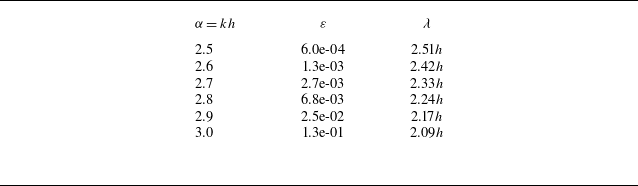
Table 1 shows the values of the dispersion errors shown in figure 1 in the vicinity of the limiting value
 $kh=\pi$
, and the wavelengths resolved by the scheme corresponding to these errors.
Values of the dispersion errors and the corresponding wavelengths resolved by the scheme.

Judging from table 1, and assuming dispersion error
 $0. 00 68$
, the minimal values of the resolved wavelengths can be formally estimated as
 $2.24h$
. Considering such an estimate as quite satisfactory, we will further assume that the multi-operator chosen in this way is used to approximate the derivatives. The errors for other considered approximations, as can be seen, significantly exceed the errors of the multi-operators, and have narrower intervals of
 $kh$
, where they are visually small. This provides a basis for reproducing smaller scales of turbulence in numerical solutions.
2.1.1. Dissipative multi-operator
The multi-operator
 $D_M$
in (2.3) looks like
 \begin{align} D_{M}( \bar c_{1},\bar c_{2},\ldots ,\bar c_{M})= \sum _{i=1}^{M}\bar \gamma _{i}\,d(\bar c_{i}),\quad \sum _{i=1}^{M}\bar \gamma _i=1. \end{align}
The basis operators
 $d(\bar c_i)$
are formed by substitutions of sets of
 $M$
values of parameter
 $\bar c$
into a one-parameter family of operators written in terms of operators
 $L_{l}(c)$
and
 $L_{r}(c)$
in (2.4) as
 \begin{align} d(c)=L_{l}(c)-L_{r}(c). \end{align}
It can be shown that the operator
 $d(c)$
is a self-adjoint operator approximating the second derivative. Unlike
 $L_M$
, coefficients
 $\bar \gamma _i$
are determined from the conditions of vanishing of the lowest
 $M-1$
terms in the Taylor series for function
 $u(x)$
. Thus the action of a multi-operator on a smooth function approximates its
 $2M$
th-order derivative multiplied by
 $h^{2M-1}$
.
Since the basic operators are self-adjoint, the operator
 $D_M(\bar c_{1},\bar c_{2},\ldots , \bar c_{2})$
is also self-adjoint. However, it is not necessarily non-negative, as required by the stability of the scheme. Therefore, there is a restriction on the choice of values
 $(\bar c_{1},\bar c_{2},\ldots , \bar c_{2})$
based on the requirement that the Fourier transform of the operator
 ${\hat D}_M$
be positive. To ensure that this requirement is met, parameters
 $\bar c_{i}$
are assumed to be uniformly distributed between their minimum and maximum values
 $\bar c_{\textit{min}},\bar c_{\textit{max}}$
. Then the admissible parameters will be considered to be the parameters for which function
 $d(kh)={\hat D}_M(kh;\bar c_{\textit{min}},\bar c_{\textit{max}})$
is positive.
Unlike the rigidly fixed values
 $c_{\textit{min}}, c_{\textit{max}}$
, they are free parameters that allow one to control the spectral properties of the dissipation within the framework of the scheme.
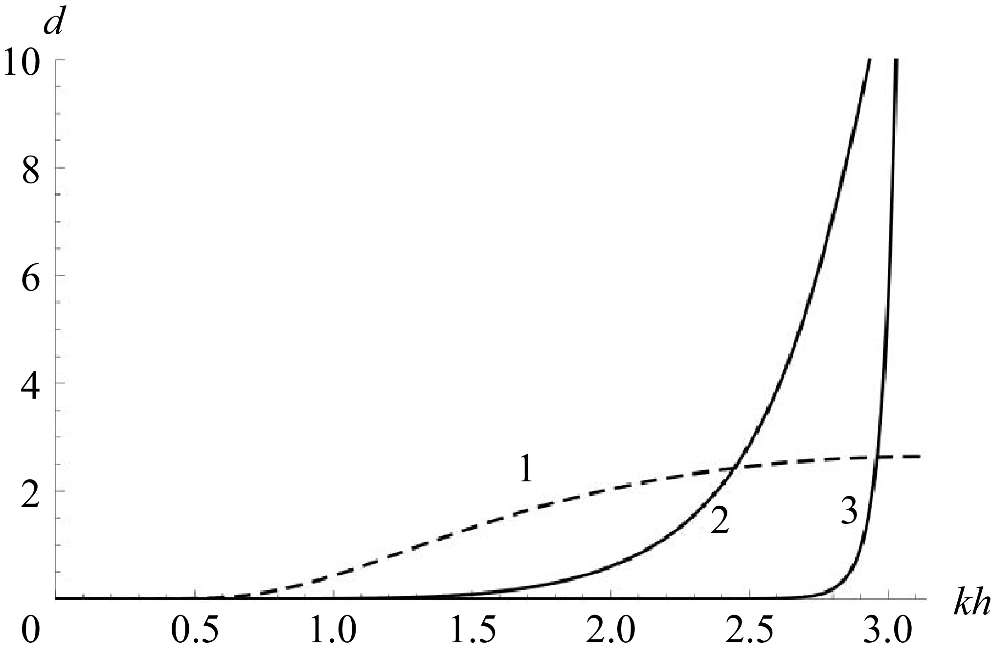
Figure 2 shows variants of the functions
 $d(kh)$
corresponding to different values
 $\bar c_{\textit{min}},\bar c_{\textit{max}}$
. They all have the same asymptotics
 $d=O(\alpha ^{23}),\ \alpha =kh$
, but different intervals
 $kh$
, on which the graphs of these functions are visually close to the abscissa. In the case of curves 1, 2, 3, the actions of the dissipative multi-operator on the Fourier harmonics turn out to be very small at
 $kh\lesssim 0.6$
,
 $kh\lesssim 1.5$
,
 $kh\lesssim 2.7$
, respectively. For brevity, in what follows we will denote the operators corresponding to curves 1, 2, 3 as dissipations 1, 2, 3, respectively.
Spectra of dissipative operators; curves 1, 2, 3 correspond to three different pairs of free parameters.

The term with dissipative operator
 $D_M$
in (2.3) can be considered as an approximation of some source added to the original equation. In the case of its stable solutions, functions
 ${\hat D}_M(kh)$
and constant
 $C$
can only affect the monotonic properties of the numerical solutions in the presence of large gradients. However, in the case of unstable exact solutions, despite the contribution of the order of
 $O(h^{23})$
to the approximation error, this source is a small disturbance capable of exciting unstable modes. Then its spectral properties can significantly affect the formation of numerical solutions describing the emerging non-stationary solutions regimes. This was confirmed in the case of the excitation of Tollmien–Schlichting waves in the flat plate boundary layer (Tolstykh & Shirobokov Reference Tolstykh and Shirobokov2020).
The main results presented in this study are obtained using dissipation 2 from figure 2. Limited calculation data for dissipation 1 are given below to confirm the role of controlled dissipation.
2.1.2. Application to the Navier–Stokes equations
The inviscid part of the Navier–Stokes equations was approximated according to the scheme using the approximations of the derivatives and dissipative component described above. To approximate terms with viscosity assumed to be independent on temperature, three-point central differences were used. Preliminary calculations using compact fourth-order approximations showed that we do not expect the second order of these differences at large Reynolds numbers to have a noticeable effect on the structure of the resulting solutions, but it significantly simplifies parallel codes for supercomputer calculations. The semi-discrete scheme constructed in this way is stable in the
 $L_2$
norm in the frozen coefficient approximation. The fourth-order Runge–Kutta method used as the time stepping procedure makes it conditionally stable. Methodical calculations have shown that in the case of sufficiently small time steps, natural for describing non-stationary processes, the accuracy of spatial approximations is not compromised.
2.1.3. Parallel implementation
In parallel implementation of the described algorithm, the key point is that the main computational time costs are associated with numerous inversions of bidiagonal matrices by means of so-called ‘runnings’ computations with left sweeps and similar right sweeps, independent of each other. Using this property of the above-described multi-operators, in Lipavskii & Konshin (Reference Lipavskii and Konshin2022) a parallel code implementing the scheme in the case of the Euler equations is described, with the main attention paid to the study of its message passing interface (MPI) implementation. In the present study, the code was extended to the case of the Navier–Stokes equations without noticeable changes in its parallel efficiency. The parallel efficiency of the current MPI + OpenMP implementation turned out to be very close to ideal when using up to 1024 computational cores.
2.2. Problem formulations
Numerical solutions of the Navier–Stokes equations describing unsteady flows in a three-dimensional subsonic unheated round jet emerging into an ambient gas at rest are considered. We assumed constant viscosity and Prandtl number equal to unity. In the calculations, the Cartesian coordinate system
 $x$
,
 $y$
,
 $z$
was used, the coordinates being normalised by the nozzle radius
 $r$
. The velocity components
 $u$
,
 $v$
,
 $w$
along the axes
 $x$
,
 $y$
,
 $z$
, and density
 $\rho$
, were normalised, respectively, by the velocity and density in the centre of the nozzle exit cross-section. The computational domain was a rectangular parallelepiped
 $0\leqslant x\leqslant 300$
,
 $-300\leqslant y\leqslant 300$
,
 $-300\leqslant z\leqslant 300$
in which the jet was directed along the
 $x$
-axis, i.e. along the line
 $y=0$
,
 $z=0$
. The work area, i.e. the part of the computational domain in which the obtained solutions were analysed, was much smaller:
 $0\leqslant x\leqslant 30$
,
 $-3.8\leqslant y\leqslant 3.8$
,
 $-3.8\leqslant z\leqslant 3.8$
. The rest of the domain was considered as sponge zones with rapidly increasing mesh sizes. For each of the spatial directions, the grid points of the
 $541\times 145\times 145$
mesh were condensed via smooth transformations in the domain of the supposed rapid change of the solutions. This gives mesh sizes in the work area that do not exceed
 $0.08$
.
Despite large mesh sizes in the sponge zones at the lateral and outflow remote boundaries (which are sufficient to absorb outgoing disturbances), characteristic non-reflecting boundary conditions were used. They were used also at the
 $x=0$
plane. In the nozzle exit area, the boundary conditions mimicking outlet flow parameters were specified. The horizontal velocity was imposed as
 \begin{align} u(r) =\frac 12 + \frac 12\tanh \left (\frac {\theta }4\left (\frac 1r-r\right )\right ), \end{align}
where
 $r$
is the radius of the nozzle, and
 $\theta =50$
. The pressure was assumed to be equal to its ambient value. The internal energy and density were determined from the Crocco–Buzeman relations with the temperature ratio equal to unity and the Mach number based on the inflow axial velocity equal to
 $0.5$
. This type of the inflow conditions turned out to be sufficient to reproduce the typical structure of cold subsonic jets in numerical solutions of the Navier–Stokes equations using the considered scheme with modest mesh sizes.
The calculations were performed for two Reynolds numbers based on the nozzle radius using the standard fourth-order Runge–Kutta time stepping procedure. The initial conditions were assumed to be the flow parameters of a round jet independent of the
 $x$
-coordinate.
3. Numerical results
Starting from the initial flow field, the time stepping process included the relaxation to the statistically established unsteady regime followed by the time interval for getting statistics of that regime. Below are descriptions of the numerical solutions at the final stage of calculations, and their analysis.
3.1. Flow fields described by numerical solutions
Figure 3 shows snapshots of the vorticity norms calculated from the values of the velocity components for the Reynolds numbers equal to
 $10^3$
and
 $3\times 10^5$
, and dissipation 2. Figures 3(a,c) show the vorticity patterns in the
 $z=0$
plane, and figures 3(b,d) show their three-dimensional images. Each of these variants characterises a well-known structure of jets flowing out of nozzles with a laminar–turbulent transition. It consists of the initial stage of instability development downstream of the nozzle exit, the transition region with coherent structures, and the region of turbulent regime. These regions are most clearly represented in the case of a small Reynolds number. In the first of them, toroidal vortices formed in an extended region of the laminar regime are visible, characterising the development of the Kelvin–Helmholtz (KH) instability. In the second region, large irregular vortex structures are noticeable. In the third region, chaotic, densely packed small vortices are filled.
Snapshots of vorticity fields for two Reynolds numbers: (a,b)
 $Re=10^3$
, (c,d)
 $Re=3\times10^5$
, for (a,c) the meridional plane, and (b,d) a three-dimensional view.

As follows from figure 3, in the case of a large Reynolds number, the breakdown of the laminar regime occurs significantly closer to the nozzle exit than in the case of small Reynolds number
 $Re=10^3$
. Figure 4 shows a fragment of the vortex field for
 $Re=3\times 10^5$
from figure 3(d). It is evident that the extended region of vortex rings observed in the case
 $Re=3\times 10^5$
is absent, and large vortex structures are formed immediately after small changes in the regular flow regime.
The presented instantaneous fields characterise the general form of the solutions, which does not change significantly over time at the stage of the established turbulent regime. At the same time, as methodical calculations have shown, the solutions are sensitive to small changes in the boundary conditions at the nozzle outlet. For example, the lengths of the potential cores turn out to be noticeably different even with small changes in the specified velocity values for
 $x=0$
. It can be assumed that the geometry of the nozzle lips and other details of the boundary conditions at
 $x=0$
can also affect the solutions at their laminar stages.
Vorticity field near the nozzle exit; details as in figure 3,
 $Re=3\times 10^5$
.

In figure 5, in the plane
 $z=0$
for the same Reynolds numbers, the fields of time-averaged longitudinal velocity (figures 5
a,c) and kinetic energy of its pulsations (figures 5
b,d) are presented. The figure clearly shows the difference in the sizes of potential cores in the cases of small and large Reynolds numbers, as well as the absence of pulsations in the region of its existence. It can also be noted that the regions of maximum pulsations in all cases are located approximately immediately behind the regions of potential cores.
Time-averaged
 $x$
-velocity fields and energy of velocity pulsations for two Reynolds numbers, meridional plane: (a,b)
 $Re=10^3$
, (c,d)
 $Re=3\times 10^5$
, for (a,c) velocity, and (b,d) velocity pulsations energy.

The calculations were also performed for the Reynolds number
 $Re=3\times 10^5$
with dissipation 2 replaced by dissipation 1 (see figure 2).
A comparison of the snapshots of the vorticity fields for two dissipations and the time of the vortex fields of figure 3 is shown in figure 6. While maintaining the general structure of the solutions, a significant delay in the transition to the stochastic regime is noticeable. Such a change in the solution confirms the influence of the dissipative mechanism and consequently the possibility of using it for partial control of the type of solutions.
Influence of numerical dissipation. Snapshots of vorticity fields in the cases (a,b) dissipation 2 and (c,d) dissipation 1 from figure 2. Here,
 $Re=3\times 10^5$
.

It is interesting to note that the study Shur et al. (Reference Shur, Spalart and Strelets2005) presents comparisons of the jet vorticity fields obtained within the framework of ILES (i.e. when solving the Navier–Stokes equations without SGS models) using two dissipative schemes of the third and fifth orders. It turned out that in the case of a more dissipative scheme of the third order, the transition occurred at larger distances from the nozzle. This fully corresponds to the observed effect of dissipation 1, which is more intense compared to dissipation 2 in the actual range of wavenumbers. This is also consistent with the diversity of the sizes of potential cores obtained when using different versions of the LES schemes.
As for the effect of using dissipation 1, its explanation possibly looks as follows. The excited instability waves have relatively small wavenumbers. The action of dissipation operator 2 in the Fourier space has virtually no effect on harmonics of this type; only the natural viscous dissipation operator acts on them. This effect is small due to the high Reynolds number. In the case of dissipation 1, the spectrum of the dissipation operator is shifted towards small wavenumbers, i.e. towards the wavenumbers of instability waves. At the same time, for such waves, the dissipation of the scheme increases. Accordingly, the range of harmonic wavenumbers with increased numerical dissipation expands, bringing the latter closer to viscous dissipation at lower Reynolds numbers.
3.1.1. Comparisons with experiments
Following the comparisons with experimental data commonly used in publications, figure 7 shows the distributions along the axis of the mean centreline axial velocity and the centreline axial velocity root mean square in the solutions obtained for Reynolds number
 $3\times 10^5$
. It also shows the experimental data for the inflow parameters that are relatively close to this variant. It should be noted that the calculated and experimental data available in the literature indicate the proximity of the shapes of the curves describing them. Their main differences are associated with the different lengths of the laminar flow regions, which, for the same values of the Mach numbers and Reynolds numbers, can depend on other parameters of the flow fields (e.g. background turbulence, nozzle lips geometry). These differences seem quite explainable, since even small details can affect the development of instability both under experimental conditions and in numerical solutions. In the case of the present numerical solutions, this conclusion is confirmed by comparing the solutions obtained for dissipations of types 1 and 2 in figures 3 and 6, respectively. Taking into account the scatter of experimental data in figure 7, one can speak of agreement at a qualitative level of the solutions obtained with the experimental data. The same can be said about the comparison with LES results. The figure shows the LES curves chosen as being close enough to the calculated curves.
Comparisons of the present
 $Re=3\times 10^5$
calculations with experiments and LES calculations with more or less close inflow parameters. (a) Mean centreline axial velocity, where solid and dotted lines correspond to present calculations and calculations of Bodony & Lele (Reference Bodony and Lele2005), and triangles and circles correspond to Morris & Zaman (Reference Morris and Zaman2010) and Souza et al. (Reference Souza, Proença, de Almeida and Self2017). (b) Centreline axial velocity root mean square, where solid, dashed and dotted lines correspond to present calculations and calculations of Bodony & Lele (Reference Bodony and Lele2005) and Bogey & Bailly (Reference Bogey and Bailly2004), and triangles correspond to Lau (Reference Lau1981).

3.2. Fine details of numerical solutions near the nozzle lips
Using the large extent of the laminar regime region at low Reynolds number 1000, we consider the details of the numerical solutions at small distances from the nozzle lips.
To describe them, it makes sense to turn to the studies of small oscillations in the vicinity of the sharp leading edge of a flat plate generating the Tollmien–Schlichting waves (Tolstykh & Shirobokov Reference Tolstykh and Shirobokov2020, Reference Tolstykh and Shirobokov2022, Reference Tolstykh and Shirobokov2024). The following technique was used to detect them in the case of the longitudinal velocity
 $u(x)$
close to the surface against the background of its visually smooth variation along
 $x$
. Numerical solutions of the Navier–Stokes equations at successive time moments at small intervals
 $[a,b]$
of
 $x$
were used to construct the polynomials
 $p_n(x )$
of the best mean square approximation of degree
 $n$
, using the values at the grid nodes
 $x_1, x_2,\ldots , x_m$
.
The polynomials were constructed as a solutions to the following problem. For a given integer
 $n$
, find the coefficients of the polynomial
 $p_n(x)$
such that the condition
 $\sum _{i=1}^m(u(x_i)-p_n(x_i))^2=\min$
is satisfied. If function
 $u(x)$
is a function on which small oscillations are superimposed, then for some range
 $n$
, the polynomial turns out to be a smooth approximation to
 $u(x)$
that does not contain the extrema of these oscillations. Then the difference
 $\delta U=u(x_i)-p_n(x_i)$
can clearly reproduce the oscillations of
 $u(x)$
relative to the reference function
 $p_n(x)$
, and thereby detect their existence, as well as approximately estimate their amplitudes and wavelengths. In this case, one can geometrically imagine that the graph of
 $p_n(x)$
is the graph of some ‘average’ curve passing between the local extrema of the function
 $u(x)$
created by small oscillations superimposed on it.
However, it should be kept in mind that if
 $u(x)$
is
 $u(x,t)$
, and the extrema of the superimposed oscillations change their positions at different moments in time on the interval
 $[a,b]$
, then
 $\delta U(x_i,t)$
maps the travelling waves to a coordinate system that moves over time along with the carrier function
 $u(x,t)$
. Accordingly, if the positions of the extrema do not change over time, then the oscillations are ‘frozen’ into this function.
It turned out that the differences
 $\delta U=u(x_i)-p_n(x_i)$
in the boundary layer case can reveal very small oscillations of function
 $u$
. Due to the high accuracy of the 16th-order scheme used in Tolstykh & Shirobokov (Reference Tolstykh and Shirobokov2020, Reference Tolstykh and Shirobokov2022, Reference Tolstykh and Shirobokov2024), it was possible to isolate oscillations with amplitudes of the order of
 $10^{-7}$
. These oscillations in the immediate vicinity of the sharp leading edge had the form of standing waves. As the distance from the edge increased to a certain value
 $x$
(i.e. to a certain Reynolds number based on the displacement thickness), in full accordance with the linear theory, wave packets were observed moving downstream with increasing amplitudes. Estimates of the wavenumbers of their fillings showed that they are inside the instability diagram and are the Tollmien–Schlichting waves. Estimates of the amplitude growth rate confirmed this fact. Based on these observations, it was concluded that the boundary conditions discontinuity at the sharp leading edge in the solutions of the Navier–Stokes equations is one of the instability triggers. But at the same time, as calculations with dissipation with a different spectrum showed, the main exciter of instability is the dissipative mechanism (Tolstykh & Shirobokov Reference Tolstykh and Shirobokov2022).
In the numerical solutions under consideration, the role of the sharp edge is played by the nozzle lips, where the derivative of the longitudinal velocity in the radial direction undergoes a discontinuity due to the boundary conditions at
 $x=0$
. Below are some results of the above solutions processing in the region
 $x\lt 14$
, preceding the region of coherent structures.
Figure 8 shows the velocity profiles
 $u(x)$
in the shear layer (
 $x\in [0,14], y=1, z=0$
) at three successive times. They characterise the downstream propagation and growth of the KH waves. The curve displacements allow one to roughly estimate their downstream velocity.
Instability waves in the shear layer,
 $Re=1000$
:
 $u$
-velocity distributions along the upper lipline at
 $t=t_1$
(black),
 $t_2=t_1+0.4$
(blue),
 $t_3=t_1+0.8$
(red).

Taking into account the arbitrariness in visually determining the position of the curve extrema, rough estimates give values of approximately 0.5–0.6. However, using the method described above allows us to establish that these waves carry shorter waves with small amplitudes. To detect them, the main interval
 $x$
was divided into two intervals
 $[0,7]$
and
 $[7,14]$
. For each of them, the polynomials
 $p_n(x)$
were constructed with the Chebyshev polynomials as basis functions.
Figure 9 shows the deviations
 $\delta U(x)$
of the numerical solutions from
 $p_n(x)$
at the times corresponding to the graphs of figure 8. In the interval
 $[0,7]$
, oscillations with very small amplitudes are visible, visually indistinguishable for the time moments considered. They are similar to the oscillations in the immediate vicinity of the sharp leading edge of the plate, and are apparently associated with a discontinuity of the radial derivative of velocity
 $u$
in the boundary conditions at the nozzle lips. In the interval
 $[7,14]$
, where the critical Reynolds number for the shear layer thickness is presumably reached, oscillations of
 $\delta U(x)$
that are different for each time are observed. They show wave packets travelling downstream with increasing amplitudes. A rough estimate of the velocity extrema movement obtained from the graphs yields a value approximately 0.4–0.5. Thus the small oscillations in the vicinity of the nozzle lips look like additional exciters of KH waves.
Small-amplitude waves carried by instability waves. Deviations
 $\delta U$
from the reference polynomials approximating functions displayed in figure 8: black
 $t=t_1$
, green
 $t=t_2$
, blue
 $t=t_3$
, for
 $x$
-intervals (a)
 $[0,7]$
and (b)
 $[7,14]$
.

The amplitudes of the generated waves are small compared to the amplitudes of the main waves, and their role in shaping the jet structure can be expected to be less significant. Based on the visualisation results of these instability waves, it can be concluded that at short distances from the nozzle exit, they are simply carried by the main KH waves. However, as their amplitudes increase downstream, nonlinear interactions can be expected. Unfortunately, it is difficult to extract information about these complex processes from the obtained solutions, and to evaluate how the influence of nozzle lips waves on the jet parameters is reflected in the numerical solutions. Additional calculations are required for this.
A separate issue beyond the scope of this study is the nozzle lips influence on the formation of trapped waves in the potential core of the jets.
3.3. Statistical properties of solutions
One of the important tools for studying the stochastic properties of numerical solutions is the calculation of correlation functions. In this study, by averaging over a sufficiently wide time interval of the steady-state non-stationary regime, the temporal autocorrelations of the axial velocity
 $u(x,t)$
and its autocorrelation coefficients were calculated for different axial positions using formulas of the form
 $B(x,\tau )=\overline {u(x,t)\,u(x,t+\tau )}$
,
 $R_{uu}=B(x,\tau )/B(x,0)$
, where the overbar denotes averaging over an interval
 $t \in [0,T]$
.
The spatial autocorrelation function
 $B(\delta ,t) =\overline {u(x+\delta ,t)\,u(x,t)}$
and the corresponding autocorrelation coefficients
 $R_{uu}$
were also calculated. In the case of the Taylor frozen turbulence hypothesis, these correlations should coincide if we set
 $\delta =\bar u \tau$
. Taking into account such a transformation, figure 10 shows both coefficients of these correlations for the value of
 $x$
in the region of chaotic small eddies at
 $Re=3\times 10^5$
, and the time value at the late stage of calculations. From these graphs it follows first, that the shape of the autocorrelation curves is typical for developed turbulent flows, and second, that the frozen turbulence hypothesis is perfectly fulfilled. The symmetry of the curves relative to the origin also indicates the homogeneity of the turbulence in the direction of the
 $x$
-axis.
Comparison of temporal (solid line) and spatial (dashed line) coefficients of the
 $U$
-velocity autocorrelations.

Figure 11 shows the correlation functions calculated for the sequences of
 $x$
-values in the solutions for two Reynolds numbers. These values are chosen in both cases in the regions of coherent structures and developed turbulence.
Axial velocity autocorrelations for two Reynolds numbers: (a)
 $Re=10^3$
and (b)
 $Re=3\times 10^5$
.

According to figure 11, for smaller distances from the nozzle in the regions of coherent structures, the shapes of these functions for small
 $\tau$
are close to the shapes from figure 10 but have oscillating ‘tails’. This indicates that the solutions combine random modes and deterministic modes of the instability waves. With increasing distances from the nozzle, these ‘tails’ decrease in length, and in the regions of developed turbulence they completely disappear.
Using the calculated temporal autocorrelation functions, their Fourier transforms
 $E(\omega )$
were obtained at fixed points on the
 $x$
-axis. They give the energy spectra since
 $B(x,0)=\overline {(u^{\prime })^2}=\int _0^{\infty }E(\omega )\,\mathrm{d}\omega$
. Figure 12 shows the energy spectrum
 $E(\omega )$
calculated at
 $x=20,\ y=0,\ z=0$
in the case
 $Re=3\times 10^5$
. As a sign of a turbulent regime at that Reynolds number, the ‘
 $-5/3$
’ law line is shown in the figure. In the spectrum, the maximum value of the dimensionless frequency
 $\omega$
(calculated using the nozzle radius as the length scale) reaches a value approximately equal to
 $20$
. It gives value
 $40$
and corresponding Strouhal number approximately
 $6.5$
when using the diameter instead of the radius. Having in mind the relatively coarse mesh used, that value can be compared with the following estimates of the Strouhal numbers of the acoustic spectra in the review of LES results by Bodony & Lele (Reference Bodony and Lele2008): ‘At present, we are capable of predicting frequencies up to
 $Sr \approx 1.5{-}3.0$
, depending on the flow condition. To be more useful to frequency-weighted measurements, we need to get to Strouhal numbers closer to eight’.
The autocorrelation function allows one to calculate the Taylor microscale
 \begin{align} \lambda _t = \left (\frac 12\int _0^{\infty }\frac {B(\tau )}{B(0)}\,\mathrm{d}\tau \right )^{-1/2}. \end{align}
Figure 13 shows its distribution along the
 $x$
-axis in the high Reynolds number case. For comparison, the minimal wavelength resolved by the scheme is also shown in the figure. It corresponds to value
 $kh=2.7$
in table 1.
Energy spectrum in the turbulent region,
 $Re=3\times 10^5$
.

4. Summary and discussion
The paper presents numerical solutions of the Navier–Stokes equations for the subsonic turbulent jets problem with synthetic inflow conditions. They were obtained using a new highly accurate scheme with 24th-order multi-operators approximations. This scheme is characterised by high resolution achieved as a result of optimisation using its free parameters. In this case, the dispersion error of the approximations for dimensionless wavenumbers
 $kh=2.8$
, where
 $h$
is the mesh size, is of the order of
 $0.007$
. With this estimate, the minimum wavelength resolved by the scheme is formally approximately
 $2.2h$
.
The Taylor temporal microscale (line 1) and the minimal resolved wavelength (line 2).

An important feature of the scheme is the presence of added positive self-adjoint multi-operators, which contribute
 $O(h^{23})$
to the approximation error, and define a controlled dissipative mechanism. It can be considered as an analogue of the dissipative mechanism in LES or ILES-type schemes in which dissipation is introduced as a sub-grid modelling or is contained directly in the scheme. It can be assumed that the role of such a mechanism with a broadband spectrum is similar to the role of background turbulence in the excitation of unstable modes leading to a turbulent regime. An example is presented showing that the use of a dissipation multi-operator with different spectral properties while maintaining the general structure of the flow field changed the length of the potential core. However, a detailed study of the influence of the dissipation spectra specified in the scheme, and the constant controlling its intensity, on the numerical solutions requires additional calculations. It is beyond the scope of this paper. Questions remain open about the extent to which the numerical solutions can mimic the presence of background turbulence of various types.
The presented numerical solutions were obtained without any artificial excitation and other additional settings. They reproduce the well-known structure of subsonic jets at sufficiently high Reynolds numbers with regions of the KH waves, transition regions of coherent structures, and regions of developed turbulence.
The averaged characteristics of the flow fields were within the scatter of the experimental data and numerical solutions based on the LES schemes. Such a scatter seems natural in view of the influence on numerical solutions of even small details of both the wind tunnel experiments and the schemes used.
An analysis of the numerical solutions in the vicinity of the nozzle lips at
 $Re=1000$
showed that the KH waves carry wave packets of very low intensity (deviations from the carrier waves are of the order of 0.001–0.0001). Taking into account a similar analysis of the previously obtained numerical solutions of the Navier–Stokes equations in the vicinity of the sharp leading edge of a flat plate, it can be assumed that the source of these waves is the sharp nozzle lips in the formulation of the inflow conditions. At some distance from the nozzle, they become unstable, forming an ‘additional’ source of KH waves. Their consequence is also trapped waves in the potential core. Their analysis requires further research and is beyond the scope of the present paper.
The paper presents the results of statistical analysis of the solutions. Calculation of the autocorrelation functions of velocity in the turbulent regime region at the large Reynolds number showed not only their typical form for turbulent flows but also excellent fulfilment of the Taylor hypothesis of frozen turbulence. The calculated autocorrelations made it possible to see the difference between the solutions in the region of coherent structures and developed turbulence for small and large Reynolds numbers. Based on them, the values of Taylor microscales for the larger Reynolds number are presented.
The discrete Fourier transform of the autocorrelation functions was used to calculate the turbulent energy spectra, which showed the fulfilment of the
 $-5/3$
law. In the presented spectrum, the cut-off value of the dimensionless frequency based on the nozzle diameter is approximately
 $40$
, which gives Strouhal number approximately
 $6.5$
. That value is expected to increase when using lesser mesh sizes. Referring to the review paper of Bodony & Lele (Reference Bodony and Lele2008), the Strouhal number for acoustic spectra in LES calculations does not exceed
 $3$
. Together with the theoretical estimates of the dispersion errors of the present scheme, this indicates the possibility of its applications with sufficiently deep penetration into small scales of turbulence.
In conclusion, we note that in this study, the simplest formulation of the problem was used, in which the synthetic inflow data completely determined the flow structure with the establishment of turbulence at different distances from the nozzle exit. This formulation can be complicated by adding to it certain details that are characteristic of real flows. Such details can be e.g. the geometry of the nozzle lips. Another example is the situation when the flow is already turbulent at the nozzle exit. In this case, following the accepted principle of using the Navier–Stokes equations, it would be necessary to include at least a part of the internal region of the nozzle in the computational domain; reasonable imitations of the internal turbulent flow are also possible. All this requires additional research. In all cases, it can be expected that the use of highly accurate schemes and reasonably detailed meshes creates good opportunities both for studying turbulent regimes and for solving real problems.
Acknowledgements
The research was carried out using the infrastructure of the Shared Research Facilities ‘High Performance Computing and Big Data’ (CKP ‘Informatics’) of FRC CSC RAS (Moscow).
Declaration of interests
The authors report no conflict of interest.