2. A hidden technical implication

Assume that the minimum wage is indexed to half the average wage of the previous year. Let $ {\overline{w}}_t $ be the average monthly wage in year $ t $ . Thus, for year $ t+1 $ , the minimum wage will be set to $ \frac{{\overline{w}}_t}{2} $ . It follows that those who earned less in year $ t $ will receive this amount in year $ t+1 $ , ceteris paribus. But this means that the average wage will rise above $ {\overline{w}}_t $ (i.e. $ {\overline{w}}_t<{\overline{w}}_{t+1} $ ), therefore another minimum wage increase will be needed in year $ t+2 $ to strive to reach the 50-percent ratio. This is a system of recurrence relations, where equation $ i $ is

(1) $$ {w}_{i,t+1}=\max \left\{{w}_{i,t},{\overline{w}}_t\theta \right\}=\max \left\{{w}_{i,t},\frac{{\sum \limits}_{j=1}^n{w}_{j,t}}{n}\theta \right\}, $$

where $ {w}_{i,t} $ is the wage of worker $ i $ , $ n $ is the number of workers, and $ \theta $ is the min-to-average target ratio (0.5 in our example).

Let us take a simple example. There are five workers in the economy with 500-, 1000-, 2000-, 3000- and 3500-euro wages at $ t=0 $ . The average wage is 2000 euros, the minimum wage is 500 euros. A target ratio of 0.5 is declared. Thus, for the next year ( $ t=1 $ ), the minimum wage is set to $ {\overline{w}}_0\theta =2000\cdot 0.5=1000 $ euros. The process described above begins: a worker’s wage at $ t=1 $ will be the higher of (i) his wage at $ t=0 $ and (ii) half the average wage at $ t=0 $ (see Equation 1). The initial wage distribution is such that, in the first year, the process only affects the wage of the first worker ( $ {w}_{1,0}=500<{\overline{w}}_0\theta =1000={w}_{2,0} $ ). Ceteris paribus, the limit of the recurrence sequence (i.e. when the first worker’s wage reaches half the average wage) is

(2) $$ \underset{t\to \mathrm{\infty}}{\lim }{w}_{1,t}=\underset{t\to \mathrm{\infty}}{\lim}\frac{w_{1,t}+{w}_{2,0}+{w}_{3,0}+{w}_{4,0}+{w}_{5,0}}{5}\cdot 0.5 $$

$$ 10\underset{t\to \infty }{\lim }{w}_{1,t}=\underset{t\to \infty }{\lim }{w}_{1,t}+{w}_{2,0}+{w}_{3,0}+{w}_{4,0}+{w}_{5,0} $$

$$ \underset{t\to \mathrm{\infty}}{\lim }{w}_{1,t}=\frac{w_{2,0}+{w}_{3,0}+{w}_{4,0}+{w}_{5,0}}{9}, $$

which, after substituting concrete values, is

$$ \underset{t\to \infty }{\lim }{w}_{1,t}=\frac{1000+2000+3000+3500}{9}=1055.\dot{5}. $$

Since $ {w}_{2,0}<1055.\dot{5} $ , it follows that without the ceteris paribus assumption, the initially second-lowest wage would also increase at some point of the process. It also follows that (at least) the two lowest wages would eventually be equal. Therefore, by removing the restriction on $ {w}_{2,0} $ in Equation 2 and substituting $ \underset{t\to \infty }{\lim }{w}_{2,t}=\underset{t\to \infty }{\lim }{w}_{1,t} $ , we get

$$ \underset{t\to \mathrm{\infty}}{\lim }{w}_{1,t}=\underset{t\to \mathrm{\infty}}{\lim}\frac{2{w}_{1,t}+{w}_{3,0}+{w}_{4,0}+{w}_{5,0}}{10} $$

$$ 10\underset{t\to \infty }{\lim }{w}_{1,t}=\underset{t\to \infty }{\lim }2{w}_{1,t}+{w}_{3,0}+{w}_{4,0}+{w}_{5,0} $$

$$ \underset{t\to \mathrm{\infty}}{\lim }{w}_{1,t}=\frac{w_{3,0}+{w}_{4,0}+{w}_{5,0}}{8}, $$

which, after substituting concrete values, is

$$ \underset{t\to \infty }{\lim }{w}_{1,t}=\frac{2000+3000+3500}{8}=1062.5. $$

The new wage structure in the economy would be 1062.5, 1062.5, 2000, 3000 and 3500 euros with an average of 2125 euros. As $ \frac{2125}{2}=1062.5<{w}_{3,0} $ , the system is converged, that is reached its steady state.

It is easy to see that any change in the wage ratios triggers such an iterative process. That is, it arises whenever the growth rates of individual wages differ, which happens all the time. Consequently, this is a permanent issue.

3. A simulated example

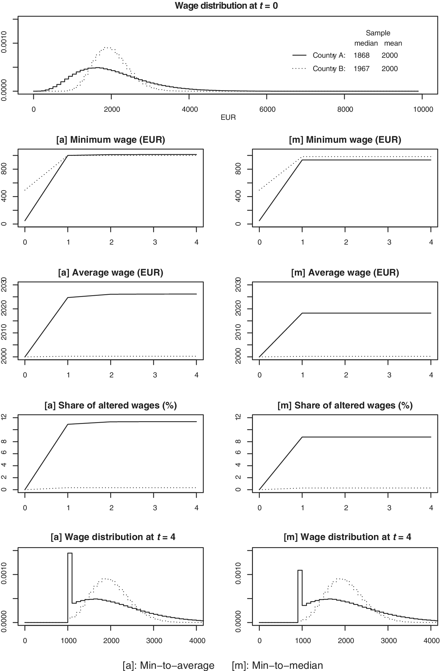
Let us simulate the outcome for two hypothetical countries. Assume that, in year 0, country A has a right-skewed wage distribution, Gamma(5, 400), while country B has a more symmetric one, Gamma(10, 200). I draw a sample of one million from each distribution; the probability densities with 100-euro bins are shown at the top of Figure 1. The average of both samples is $ {\overline{w}}_0\approx 2000 $ euros, agreeing with the theoretical value, i.e. the product of the shape and scale parameters of the gamma distribution (there is no closed-form expression for the median). The median, which is the level that splits the ascending order of wages into half, is of course lower in country A than in country B. In addition to the case of min-to-average indexing, I also examine the case of min-to-median indexing. For better comparability, I assume 50-percent ratio in both cases ( $ \theta =0.5 $ ). This gives a total of 4 scenarios (2 countries ∙ 2 indexing), the simulation results of which are shown in Figure 1.

Figure 1.

Simulation results for $ \theta =0.5 $ .

Figure 1. Long description

The figure consists of nine panels. A legend indicates Country A is a solid line and Country B is a dotted line.

1. Top Panel: Wage distribution at t equals 0. The x-axis is E U R from 0 to 10000. Both countries show a mean of 2000. Country A has a median of 1868 and a wider, lower peak. Country B has a median of 1967 and a taller, narrower peak.

2. Second Row: Minimum wage in E U R. Left panel [a] Min-to-average and right panel [m] Min-to-median. Both show a sharp linear increase from t equals 0 to t equals 1, then plateau. In [a], Country A and B converge. In [m], Country B remains slightly higher than Country A.

3. Third Row: Average wage in E U R. In [a], Country A increases from 2000 to approximately 2025, while Country B remains flat at 2000. In [m], Country A increases to approximately 2018, while Country B remains flat.

4. Fourth Row: Share of altered wages in percent. In [a], Country A rises to 11 percent while Country B stays near 0. In [m], Country A rises to 9 percent while Country B stays near 0.

5. Bottom Row: Wage distribution at t equals 4. Both panels [a] and [m] show a new sharp vertical spike for Country A at the 1000 E U R mark, representing the implementation of a minimum wage, while the rest of the distribution remains similar to t equals 0.

3.1. Min-to-average indexing

As the mean of the two initial wage distributions are equal (2000 euros), the minimum wage rose to 1000 euros in both countries in the first year. However, there is a huge difference in the number of workers affected and the size of their wage increments, and thus the cost pressure exerted on the economy. In country A, more than 10 percent of the workers received raises of varying degrees, some several times their previous wages, while in country B, less than half a percent of the workers were affected, and at best they take home about double. Moreover, after year 1, an infinite convergence of the variables to their new equilibrium levels begins. True, the lion’s share of this will take place within a year or two.

As a result, the average wage will increase by $ \underset{t\to \infty }{\lim }{\overline{w}}_t^{\mathrm{A}}-{\overline{w}}_0=26.2 $ euros in country A, which average surplus is built into the wages forever. To quantify the present value of this amount, we need to divide it into two parts. In the first year, the rise is $ {\overline{w}}_1^{\mathrm{A}}-{\overline{w}}_0=24.7 $ euros, while the rise beginning from the second year to full convergence is $ \underset{t\to \infty }{\lim }{\overline{w}}_t^{\mathrm{A}}-{\overline{w}}_1^{\mathrm{A}}=1.5 $ euros. Recall that the aftershock largely subsides by the second year, i.e. $ \underset{t\to \infty }{\lim }{\overline{w}}_t^{\mathrm{A}}\approx {\overline{w}}_2^{\mathrm{A}} $ . Thus, for simplicity, calculating with the annual sums ( $ 24.7\cdot 12=296.4 $ and $ 1.5\cdot 12=18 $ euros) and a 5 percent annual discount rate, the average present values areFootnote ⁵

$$ \mathrm{PV}\left(\mathrm{first}\ \mathrm{rise}\right)=\frac{296.4}{1.05}+\frac{296.4}{1.05^2}+\cdots =\frac{296.4}{0.05}=5928 $$

$$ \mathrm{PV}\left(\mathrm{aftershock}\right)\approx \frac{18}{1.05^2}+\frac{18}{1.05^3}+\cdots =\frac{18}{0.05}/1.05=342.9, $$

i.e. about 6271 euros per worker.

Note that aftershocks also occur if the indexation is less frequent (e.g. every 4 years, which is the maximum window allowed by the Directive, Article 5(5)). In this case, the present value of aftershocks is reduced because of the delayed convergence, which of course only means that this slice of the problem is ‘elegantly’ postponed to later years.

4. Estimating impact on the EU

The present values per worker in the above example may not seem a lot, but at the level of millions it is a visible amount. To get an idea of the scale, let us estimate the impact on each member state and thus the EU as a whole.

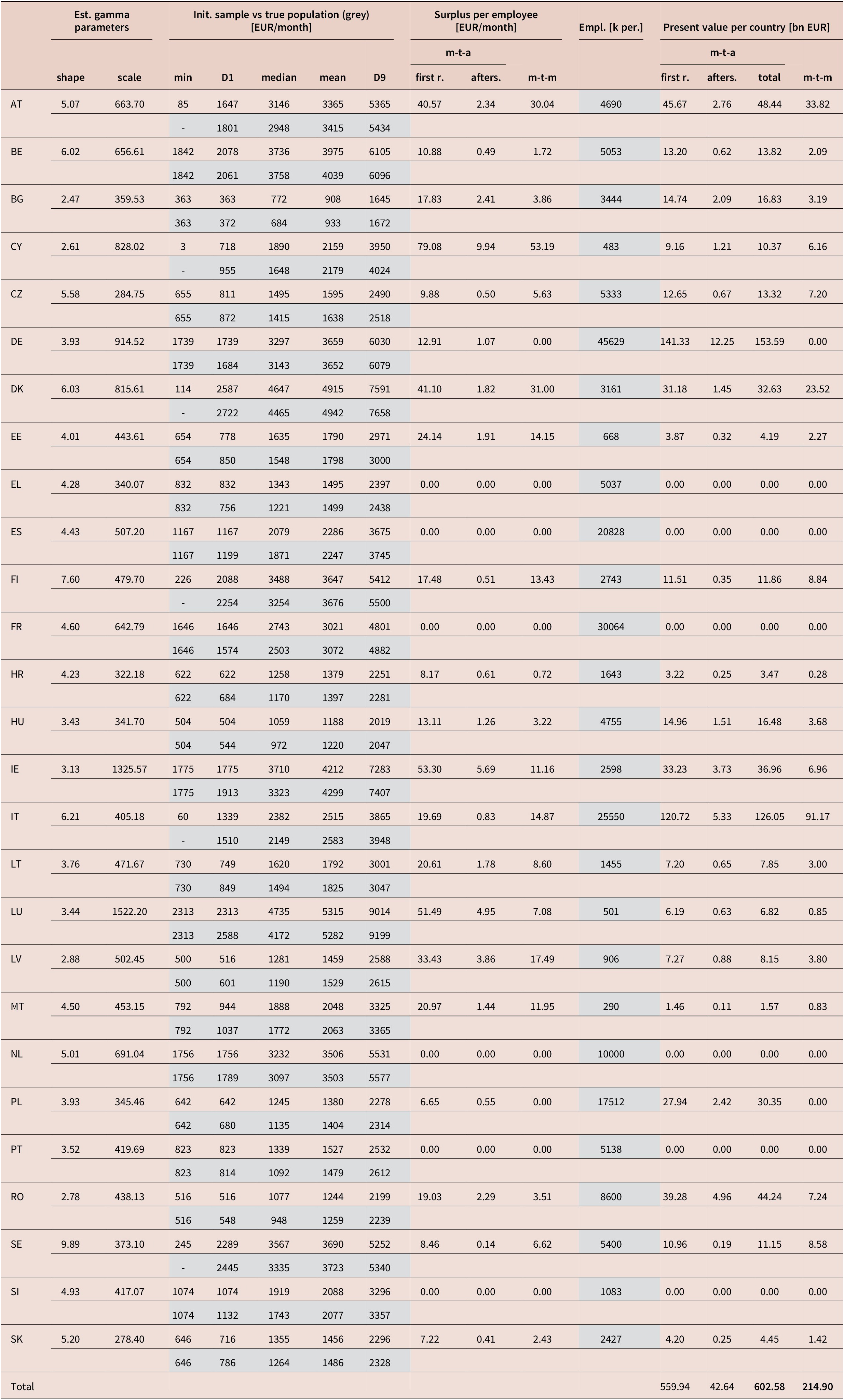
Every 4 years Eurostat publishes some distributional characteristics of the monthly earnings, such as first and ninth deciles, median (i.e. fifth decile) and average. Using the latest available data for industry, construction and services except public administration, defence and compulsory social security (Eurostat, 2022a, in euro, full-time equivalent), I prepare the country-specific wage samples as follows. I fit gamma distributions by minimising loss function

$$ \mathrm{L}\left({D}_1,{D}_5,{D}_9\right)={\left({D}_1-{D}_1^{\ast}\right)}^2+{\left({D}_5-{D}_5^{\ast}\right)}^2+{\left({D}_9-{D}_9^{\ast}\right)}^2, $$

where $ {D}_1 $ , $ {D}_5 $ and $ {D}_9 $ are the first, fifth and ninth deciles (the data are marked with asterisk). I draw a sample of ten million from each resulting wage distribution. In the samples of 21 countries that already had a minimum wage in 2022, I replace all items below the minimum wage with minimum wage (Eurostat, 2022b second semester). And finally, I run the simulations as discussed in the previous section. Table 1 summarises the estimated gamma parameters, the deciles of the initial samples and (for comparison) the true populations, and the simulation results. The national present value is calculated by multiplying the average employee’s present value by the number of employees in the domestic concept (Eurostat, 2022c). The Eurostat data used are highlighted in grey.Footnote ⁶

Table 1.

Simulation results for the EU (gamma distribution, $ \theta =0.5 $ , $ r=0.05 $ )

Table 1. Long description

The table presents simulation results for E U countries using a gamma distribution with theta equals 0.5 and r equals 0.05. It is structured with five primary header groups: Estimated gamma parameters (shape and scale), Initial sample versus true population in E U R per month (minimum, D 1, median, mean, and D 9), Surplus per employee in E U R per month (m-t-a first r., m-t-a afters., and m-t-m), Employment in thousands of persons, and Present value per country in billions of E U R (m-t-a first r., m-t-a afters., m-t-a total, and m-t-m).

Key data points include:

* AT (Austria): Shape 5.07, Scale 663.70, Mean 3365, Total m-t-a present value 48.44.

* BE (Belgium): Shape 6.02, Scale 656.61, Mean 3975, Total m-t-a present value 13.82.

* DE (Germany): Shape 3.93, Scale 914.52, Mean 3659, Employment 45629, Total m-t-a present value 153.59.

* FR (France): Shape 4.60, Scale 642.79, Mean 3021, Employment 30064, Total m-t-a present value 0.00.

* IT (Italy): Shape 6.21, Scale 405.18, Mean 2515, Employment 25550, Total m-t-a present value 126.05.

* PL (Poland): Shape 3.93, Scale 345.46, Mean 1380, Employment 17512, Total m-t-a present value 30.35.

The bottom row shows totals for the present value per country: m-t-a first r. 559.94, m-t-a afters. 42.64, total m-t-a 602.58, and m-t-m 214.90.

Note: Bold-face values indicate comparable totals (last two columns).

If the minimum wage is indexed to the average, the total present value for the EU is 603 billion euros, of which the aftershock itself accounts for a significant amount, 43 billion. If the minimum wage is indexed to the median, the present value is only about one-third, 215 billion euros. In both cases, some countries are not affected at all, while others are severely affected. Although these are rough estimates, they give an idea of the magnitude of the consequences. The big question is: what spillover effect will such a cost shock have on Europe’s already ailing competitiveness, or at least on the countries directly concerned?

It should be added that these numbers are conservative estimates, for two reasons. First, the calculations are based on 2022 data, while since then the unit labour cost has increased by well over 10 percent on average in the EU (Eurostat, 2025). Second, the calculation only takes into account the initial increase (that occurs upon the measure’s introduction) and, in the case of min-to-average indexing, the intrinsic aftershocks. However, this is merely a theoretical lower limit, as other spillover effects also come into play. For example, wages that are slightly higher than the minimum wage also tend to rise when the minimum wage is increased. Another important phenomenon is the faster growth of higher wages (for up-to-date US evidence on the rising income inequality, see Blanchet et al., Reference Blanchet, Saez and Zucman2022). As Section 2 showed, aftershocks always occur when the wage ratios change for whatever reasons, i.e. these spillover effects trigger continuous adjustments and thus increase costs beyond themselves. Note that there are no intrinsic aftershocks if the minimum wage is indexed to the median. Hence, in this case, spillover effects affecting wage distribution do not interact with an intrinsic adjustment mechanism.

4.1. Sensitivity to distribution and target ratio

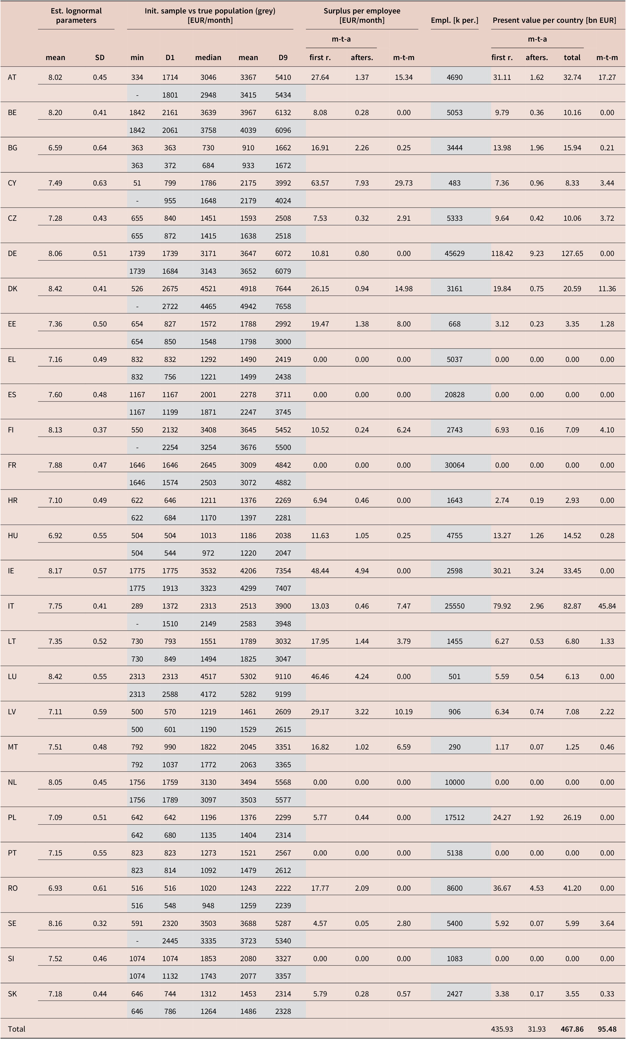
In the literature, the distribution of wages is typically characterised by lognormal distribution. This is slightly more leptokurtic than the gamma distribution. My approach is to ensure that the estimate fits the available data as close as possible considering the whole spectrum of countries. Recall that the available information includes the first, fifth and ninth deciles for each country (as well as employment data). The sensitivity analysis shows that the loss (obtained as the sum of the squared differences between the estimated values and the actual data) is smaller for every country except Belgium when using lognormal distribution; the employment-weighted loss for the EU is about 60 percent smaller.Footnote ⁷ Table 2 shows the simulation results assuming lognormal distribution.

Table 2.

Simulation results for the EU (lognormal distribution, $ \theta =0.5 $ , $ r=0.05 $ )

Table 2. Long description

The table is structured with five main header groups: Estimated lognormal parameters (mean and S D), Initial sample versus true population in grey (minimum, D 1, median, mean, D 9), Surplus per employee (m-t-a first r., m-t-a afters., and m-t-m), Employment in thousands of persons, and Present value per country in billions of E U R (m-t-a first r., m-t-a afters., m-t-a total, and m-t-m).

Key data points include:

* A T: Mean 8.02, S D 0.45, Employment 4690, Total present value 32.74.

* B E: Mean 8.20, S D 0.41, Employment 5053, Total present value 10.16.

* D E: Mean 8.06, S D 0.51, Employment 45629, Total present value 127.65.

* E S: Mean 7.60, S D 0.48, Employment 20828, Total present value 0.00.

* F R: Mean 7.88, S D 0.47, Employment 30064, Total present value 0.00.

* I T: Mean 7.75, S D 0.41, Employment 25550, Total present value 82.87.

* P L: Mean 7.09, S D 0.51, Employment 17512, Total present value 26.19.

* R O: Mean 6.93, S D 0.61, Employment 8600, Total present value 41.20.

The final Total row shows a combined m-t-a total present value of 467.86 billion E U R and an m-t-m total of 95.48 billion E U R.

Note: Bold-face values indicate comparable totals (last two columns).

Under a lognormal distribution, we get significantly smaller numbers, but the magnitude is still huge. Note that governments do not face uncertainty about the distribution, since they can run simulations on the population itself, using the complete anonymised dataset of national tax administrations.

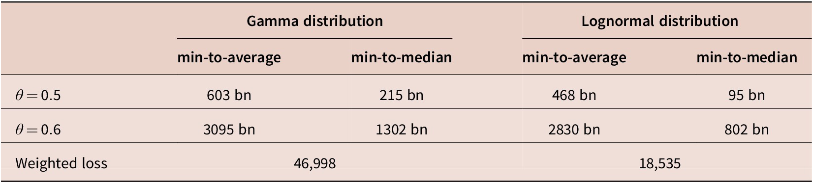
As for sensitivity to the target ratio, Table 3 shows that the cost pressure can rise quickly as the ratio increases, especially for min-to-average indexing. How do the two recommendations of the Directive relate to each other? In the case of a gamma distribution, the present value would be more than double with a 60 percent min-to-median target ratio than with a 50 percent min-to-average target ratio. With a lognormal distribution, the difference is smaller but still significant, about 70 percent. Thus, comparing the two concepts with different target ratios (i.e. min-to-median with $ \theta =0.6 $ vs min-to-average with $ \theta =0.5 $ ) may raise new dilemmas: higher cost pressure without aftershock or lower cost pressure with permanent aftershocks.

Table 3.

Sensitivity of total PV to $ \theta $ and distribution ( $ r=0.05 $ )

Table 3. Long description

The table is structured with two main distribution categories: Gamma distribution and Lognormal distribution. Each distribution is further divided into two metrics: min-to-average and min-to-median.

* Row 1: theta equals 0.5.

- Gamma distribution: min-to-average is 603 bn; min-to-median is 215 bn.

- Lognormal distribution: min-to-average is 468 bn; min-to-median is 95 bn.

* Row 2: theta equals 0.6.

- Gamma distribution: min-to-average is 3095 bn; min-to-median is 1302 bn.

- Lognormal distribution: min-to-average is 2830 bn; min-to-median is 802 bn.

* Row 3: Weighted loss.

- Gamma distribution: 46,998 (spanning both metrics).

- Lognormal distribution: 18,535 (spanning both metrics).

The constant r equals 0.05 applies to all data points.