1 Introduction
Richtmyer–Meshkov instability (RMI) ensues when a shock wave travels from a lighter (density,
 $\unicode[STIX]{x1D70C}_{1}$
) fluid to a more dense (density,
 $\unicode[STIX]{x1D70C}_{2}$
) fluid (or vice versa), with a misalignment between the shock (
 $\unicode[STIX]{x1D735}P$
) and the interface (equivalently
 $\unicode[STIX]{x1D735}\unicode[STIX]{x1D70C}$
). With an almost instantaneous deposition of vorticity along the interface due to baroclinic production from this mismatch (
 ${\sim}\unicode[STIX]{x1D735}P\times \unicode[STIX]{x1D735}\unicode[STIX]{x1D70C}$
), the interface is unstable and any small perturbations grow in time. This growth is found to be linear in time using linear analysis at the early stages, but grows nonlinearly as the perturbation amplitudes grow to the order of their wavelengths (Brouillette Reference Brouillette2002). This nonlinearly growing instability, if not dominated by the action of viscosity (high Reynolds number,
 $Re$
condition), will lead to transition to turbulence and subsequent mixing of the two fluids. This latter turbulent behaviour of RMI at high
 $Re$
occurs when the initial deposition of the vorticity is significantly large due to sufficient shock strength (large
 $\unicode[STIX]{x1D735}P$
or equivalently Mach number,
 $M$
), density mismatch of the fluid (
 $\unicode[STIX]{x1D735}\unicode[STIX]{x1D70C}$
, or equivalently Atwood number,
 $A=(\unicode[STIX]{x1D70C}_{2}-\unicode[STIX]{x1D70C}_{1})/(\unicode[STIX]{x1D70C}_{2}+\unicode[STIX]{x1D70C}_{1})$
) or misalignment of the two gradients.
Understanding this nonlinear growth transition to turbulence and the ensuing turbulent mixing of the two gases is important for many engineering applications. For example, in an attempt to ignite a fusion reaction using inertial confinement fusion (ICF) (Lindl et al. Reference Lindl, Landen, Edwards and Moses2014), a deuterium-filled fuel capsule is imploded using high energy lasers, driving the fuel to fusion-sustaining temperatures and pressures (Lindl et al. Reference Lindl, Landen, Edwards and Moses2014). The shock resulting from ablation of the fuel surface, which contains unavoidable small defects (perturbations), passes through material interfaces, leading to the occurrence of RMI. Its growth and subsequent turbulent mixing leads to the quenching of fuel and reduces the efficiency of the ignition (Zhou Reference Zhou2017a ,Reference Zhou b ). On larger application scales, understanding RMI also aids in clearing of important scientific and engineering bottlenecks in designing scramjets (Marble, Hendricks & Zukoski Reference Marble, Hendricks and Zukoski1989) and understanding supernovae (Arnett Reference Arnett2000).
The first theoretical formulation of the RMI was performed by Richtmyer (Reference Richtmyer1960), where he extended the analysis of Taylor (Reference Taylor1950) on gravity-driven Rayleigh–Taylor instability (RTI) to develop a linear growth model for RMI perturbation growth at early times. RMI was formulated as an equivalent of RTI, but with impulsive acceleration in lieu of gravity. These formulations of linear growth by Richtmyer (Reference Richtmyer1960) were verified experimentally on a shock tube by Meshkov (Reference Meshkov1969), where the gases were separated by a thin membrane (
 $1~\unicode[STIX]{x03BC}\text{m}$
) of nitrocellulose producing a nearly sinusoidal initial perturbation. Other early experiments that investigated the linear and nonlinear growth of the RMI can first be classified into two regimes – membrane and membraneless interfaces. While the membranes provide the versatility and repeatability in creation of the initial interface, it was shown by Vetter & Sturtevant (Reference Vetter and Sturtevant1995) that the effect of membrane fragments in the flow is significant at the early stages of RMI growth. The late nonlinear growth stages, however, were found to be relatively insensitive to the presence of the membrane, with the growth rates agreeing well with the theoretical predictions (Erez et al.
Reference Erez, Sadot, Oron, Erez, Levin, Shvarts and Ben-Dor2000). Most of the recent works on RMI in gases have moved towards membraneless interfaces using thin and diffuse gaseous interfaces, curtains and spherical inhomogeneities (Ranjan, Oakley & Bonazza Reference Ranjan, Oakley and Bonazza2011).
A second important consideration in studying RMI is the influence of modal content of the initial interface on the growth and mixing of the RMI. The growth of mixing width for a predominantly single-mode interface has been found to be different compared to a multi-mode interface. While imparting modal content on the interface is relatively easy using solid membranes to separate the gases, this is more complicated with membraneless experiments. Lateral oscillations have been used to generate standing waves on an interface (Jacobs & Sheeley Reference Jacobs and Sheeley1996; Jones & Jacobs Reference Jones and Jacobs1997). Removable splitter plates have also been used (Bonazza & Sturtevant Reference Bonazza and Sturtevant1996). Thin gas curtains with prescribed corrugations have been used (Balakumar et al. Reference Balakumar, Orlicz, Tomkins and Prestridge2008), and transverse shear has been imparted to perturb the interface (Weber et al. Reference Weber, Haehn, Oakley, Rothamer and Bonazza2012; Mohaghar et al. Reference Mohaghar, Carter, Musci, Reilly, McFarland and Ranjan2017). In the case of multi-mode interfaces, most are characterized as stochastic in nature as they are non-repeatable and non-uniform from experiment to experiment.
Evolution of the aforementioned interfaces has been observed in various ways as knowledge of RMI and technology evolved. The earliest of the studies on RMI have been on the growth of the perturbations and the interface growth using line-of-sight-averaged methods such as schlieren and X-ray photography. But with the advent of planar optical diagnostic techniques such as quantitative planar laser induced fluorescence (PLIF) and particle image velocimetry (PIV), recent studies have also investigated transition to turbulence and the subsequent turbulent mixing. Several works such as Orlicz et al. (Reference Orlicz, Balasubramanian, Vorobieff and Prestridge2015) have attempted to compare their results to the criterion of Dimotakis (Reference Dimotakis2005) on mixing transition in RMI. This transition is typically achieved using a sufficiently strong shock (
 $M$
) (Vetter & Sturtevant Reference Vetter and Sturtevant1995; Orlicz et al.
Reference Orlicz, Balakumar, Tomkins and Prestridge2009; Lombardini, Pullin & Meiron Reference Lombardini, Pullin and Meiron2012; Orlicz, Balasubramanian & Prestridge Reference Orlicz, Balasubramanian and Prestridge2013; Reese et al.
Reference Reese, Ames, Noble, Oakley, Rothamer and Bonazza2018), large Atwood number (
 $A$
) (Balakumar et al.
Reference Balakumar, Orlicz, Tomkins and Prestridge2008; Motl et al.
Reference Motl, Oakley, Ranjan, Weber, Anderson and Bonazza2009), modal content of initial interface perturbation (Weber et al.
Reference Weber, Haehn, Oakley, Rothamer and Bonazza2012, Reference Weber, Haehn, Oakley, Rothamer and Bonazza2014) or by using the reflected shock to perturb the RMI a second time (Balakumar et al.
Reference Balakumar, Orlicz, Ristorcelli, Balasubramanian, Prestridge and Tomkins2012; Mohaghar et al.
Reference Mohaghar, Carter, Musci, Reilly, McFarland and Ranjan2017). For example, Weber et al. (Reference Weber, Haehn, Oakley, Rothamer and Bonazza2012) observed a transition to turbulence, and a broad range of scales even before reshock using an interface with a continuous broadband spectrum perturbation consisting of structures with small separation of length scales. Alternatively, works such as Balakumar et al. (Reference Balakumar, Orlicz, Ristorcelli, Balasubramanian, Prestridge and Tomkins2012) have shown late time nonlinear growth of RMI, but transition to turbulence only after reshock. Note that the vorticity deposition from reshock will occur on a more corrugated interface and in the opposite sense (heavy to light gas) of the initial vorticity deposition. As pointed by Zhou (Reference Zhou2007), it should be noted that the mixing transition only reflects the beginning of the formation of the inertial range. The ‘minimum state’ must be achieved in order to have a sufficiently long inertial range that separates the energy-containing scale from the dissipation range. Thus, a higher Reynolds number of
 $1.6\times 10^{5}$
is required. An important goal of investigating turbulent mixing flows such as RMI is to estimate the dynamically significant quantities and aid models for computational tools (particularly Favre-averaged quantities for Reynolds-averaged Navier–Stokes (RANS) closure (Livescu & Ristorcelli Reference Livescu and Ristorcelli2008)). For example, Tomkins et al. (Reference Tomkins, Balakumar, Orlicz, Prestridge and Ristorcelli2013) investigated the terms in the evolution equation of the density self-correlation in a high-
 $A$
RMI from a near-sinusoidal curtain that is twice shocked (incident and reshock) to the turbulent mixing regime. Previous works on the current facility by Mohaghar et al. (Reference Mohaghar, Carter, Musci, Reilly, McFarland and Ranjan2017) have also observed the effect of initial condition modal content on evolution of velocity–density correlations.
On the computational front, RANS (Schwarzkopf et al. Reference Schwarzkopf, Livescu, Baltzer, Gore and Ristorcelli2016; Morgan, Schilling & Hartland Reference Morgan, Schilling and Hartland2018) and large eddy simulation (LES) (Hill, Pantano & Pullin Reference Hill, Pantano and Pullin2006; Thornber et al. Reference Thornber, Drikakis, Youngs and Williams2012) have been employed to investigate RMI in a similar sense. Schilling & Latini (Reference Schilling and Latini2010), Morán-López & Schilling (Reference Morán-López and Schilling2013, Reference Morán-López and Schilling2014) have also used weighted essentially non-oscillatory (WENO) flux reconstruction in simulations to study the variable density physics and associated evolution of turbulent kinetic energy in RMI. Latini, Schilling & Don (Reference Latini, Schilling and Don2007) and Schilling, Latini & Don (Reference Schilling, Latini and Don2007) have also shown the necessity for higher-order WENO simulations to accurately capture the instabilities inside the roll-ups in the RMI. There have also been combined computational–experimental works evaluating the computational tools (Leinov et al. Reference Leinov, Malamud, Elbaz, Levin, Ben-Dor, Shvarts and Sadot2009; McFarland, Greenough & Ranjan Reference McFarland, Greenough and Ranjan2011; Morgan et al. Reference Morgan, Aure, Stockero, Greenough, Cabot, Likhachev and Jacobs2012; McFarland, Greenough & Ranjan Reference McFarland, Greenough and Ranjan2014a ; McFarland et al. Reference McFarland, Reilly, Black, Greenough and Ranjan2015).
In the current work, the evolution, transition and turbulent mixing of a strongly shocked RMI are investigated in a late transitional/early turbulent regime. For RMI to be sufficiently strong to transition to a fully turbulent regime before dissipating, a strong deposition of baroclinic vorticity is required (high
 $M$
or
 $A$
) coupled with a long development length (
 $\equiv$
time) in the shock tube facility. To the best of the authors’ knowledge, barring the recent work of Reese et al. (Reference Reese, Ames, Noble, Oakley, Rothamer and Bonazza2018) (
 $M=2.2$
), the RMI investigation using simultaneous PLIF/PIV has typically been in the
 $M<1.6$
regime. Further, the effect of incident shock Mach number on RMI was investigated with
 $1.2<M<1.5$
in the previous experimental works which employed an initial condition of a varicose perturbed heavy gas curtain (Orlicz et al.
Reference Orlicz, Balakumar, Tomkins and Prestridge2009, Reference Orlicz, Balasubramanian and Prestridge2013, Reference Orlicz, Balasubramanian, Vorobieff and Prestridge2015). The current work is an extension of the previous efforts to study the effect of Mach number on the modal content, RMI evolution and late time behaviour of a strongly shocked density interface. We leverage the presence of a well-defined dominant mode (i.e. inclined interface) and a superposed multi-mode perturbation. Additionally, this work investigates turbulence statistics in the post-reshock regime. The following sections are organized into: first, an overview of the experimental set-up, then a thorough qualitative and quantitative investigation of the evolution of RMI, followed by analysis of large ensembles of highly resolved, simultaneous velocity–density measurements used to compute several turbulence statistics.
2 Experimental set-up
2.1 Facility
All of the experiments in the current study were performed on the inclined shock tube at the Shock Tube and Advanced Mixing Laboratory (STAM Lab). The shock tube is 9 m in total length, and can be inclined at any angle from a horizontal configuration all the way to vertical with respect to the ground. This enables sustaining of a stably stratified gas interface which is always perpendicular to the local gravitational acceleration, and inclined to the incident shock, allowing control of the shock–density-gradient misalignment. More details on the construction and instrumentation of the shock tube facility can be found in previous works (McFarland et al. Reference McFarland, Reilly, Creel, McDonald, Finn and Ranjan2014b ; Reilly et al. Reference Reilly, McFarland, Mohaghar and Ranjan2015; Mohaghar et al. Reference Mohaghar, Carter, Musci, Reilly, McFarland and Ranjan2017). Only details relevant to the current work are presented here.
Of particular relevance to the current set of experiments is the mechanism of shock generation, which allows control of the Mach number. While the driver side of the shock tube has a circular cross-section, the driven side has a square cross-section with area
 $11.43\times 11.43~\text{cm}^{2}$
, and is separated from the driver by a diaphragm which is hydraulically clamped between the two sections. An X-shaped knife edge is located below the diaphragm such that the diaphragm bulges against it when under sufficient pressure. Rapid pressurization of the driver section (via a fast-acting boost valve) leads to dynamic rupture of the diaphragm at a specific, repeatable burst pressure. Due to the sudden release of pressure, a shock front is formed which coalesces to a planar shock before impinging on the interface. Although Mach number can also be controlled by changing the gas in the driver and driven sections, in the current work it is controlled by using a different diaphragm with higher rupture pressure. A pair of pressure transducers located just above the test section and spaced 10 cm apart is used to measure the shock speed and to trigger the data acquisition systems. Further, the shock speed and rupture pressure are used to qualify the data, where, if a large variation is detected, the data are excluded from the ensemble.
Finally, because the interface is accelerated by the impinging shock, it travels down the tube. Thus, overlapping windows on either side of the shock tube between the interface location and the end wall provide optical access to investigate the entire RMI evolution as the interface translates down the shock tube. A dynamic pressure transducer at the end wall indicates the time of shock reflection from the end wall (reshock), and a pair of transducers on the side wall measures the reshock speed.
For the current work, a nitrogen stream is passed through an acetone bubbler, which is heated to control saturation temperature, and then diluted with pure nitrogen; this composes the light gas, and carbon dioxide is used as the heavy gas. This results in an effective Atwood number (
 $A=(\unicode[STIX]{x1D70C}_{2}-\unicode[STIX]{x1D70C}_{1})/(\unicode[STIX]{x1D70C}_{2}+\unicode[STIX]{x1D70C}_{1})=0.22$
, where
 $\unicode[STIX]{x1D70C}_{2}$
and
 $\unicode[STIX]{x1D70C}_{1}$
are heavy and light gas densities). A separate stream of nitrogen was used as driving gas to pressurize and rupture the diaphragm. The acetone bubbling in the lighter gas is used as a fluorescence marker to measure the concentration of the light gas, and thus the densities.
2.2 Diagnostics
To investigate the shock induced mixing between the two gases, a two-camera system was used to perform simultaneous PIV and PLIF measurements over an overlapping field of view. The PIV system consisted of a TSI PowerView 29 MP CCD camera viewing the light sheet normally and a dual-head Nd:YAG laser producing
 $532~\text{nm}$
light. The PLIF system consisted of an identical TSI PowerView 29 MP CCD camera viewing the same plane as the PIV camera, but at a slight angle in order to maintain the same pixel resolution. Thus, a Scheimpflug mount is used to adjust the plane of focus to coincide with the light sheet. A frequency quadrupled dual-head Nd:YAG Litron laser producing
 $266~\text{nm}$
UV light is used to excite the acetone in the light gas side. The laser beams are combined using beam-combining optics, passed through a spherical lens to produce a beam waist at the imaging location, then through a sheet-generating cylindrical lens and directed into the shock tube through a quartz window at the bottom of the shock tube. The sheet is aligned normal to the plane of the propagating shock and slices the inclined interface, with a measured width of approximately
 $0.7~\text{mm}$
at the beam waist. By using a
 $532~\text{nm}$
band-pass filter on the PIV camera and a
 $532~\text{nm}$
notch-filter (OD4) on the PLIF camera, the PIV and PLIF signals from the field of view are imaged separately.
The detailed evolution of the velocity and density fields as the interface translates with time is captured from an ensemble of experiments at the various interface locations by controlling the delay between shock detection and the PIV–PLIF acquisition. A calibration image is taken with both cameras each time the cameras are moved so as to register the PIV and PLIF measurements to each other.
The PIV processing is performed using TSI Insight 4G software, recursively decreasing the window size from
 $64\times 64~\text{px}^{2}$
to a final window size of
 $24\times 24~\text{px}^{2}$
. This gives a final in-plane vector spacing of
 $358~\unicode[STIX]{x03BC}\text{m}$
in each linear dimension. The PLIF processing is performed in house, where each raw PLIF image is corrected for laser intensity variations, striations and for Beer’s law attenuation. This correction is based on Weber et al. (Reference Weber, Haehn, Oakley, Rothamer and Bonazza2012, Reference Weber, Haehn, Oakley, Rothamer and Bonazza2014), and the details can be found in Mohaghar et al. (Reference Mohaghar, Carter, Musci, Reilly, McFarland and Ranjan2017). The resolution of PLIF images is
 $68~\unicode[STIX]{x03BC}\text{m}~\text{pixel}^{-1}$
. Finally, in order to measure density–velocity cross-statistics, PLIF images and PIV data are registered (Mohaghar et al.
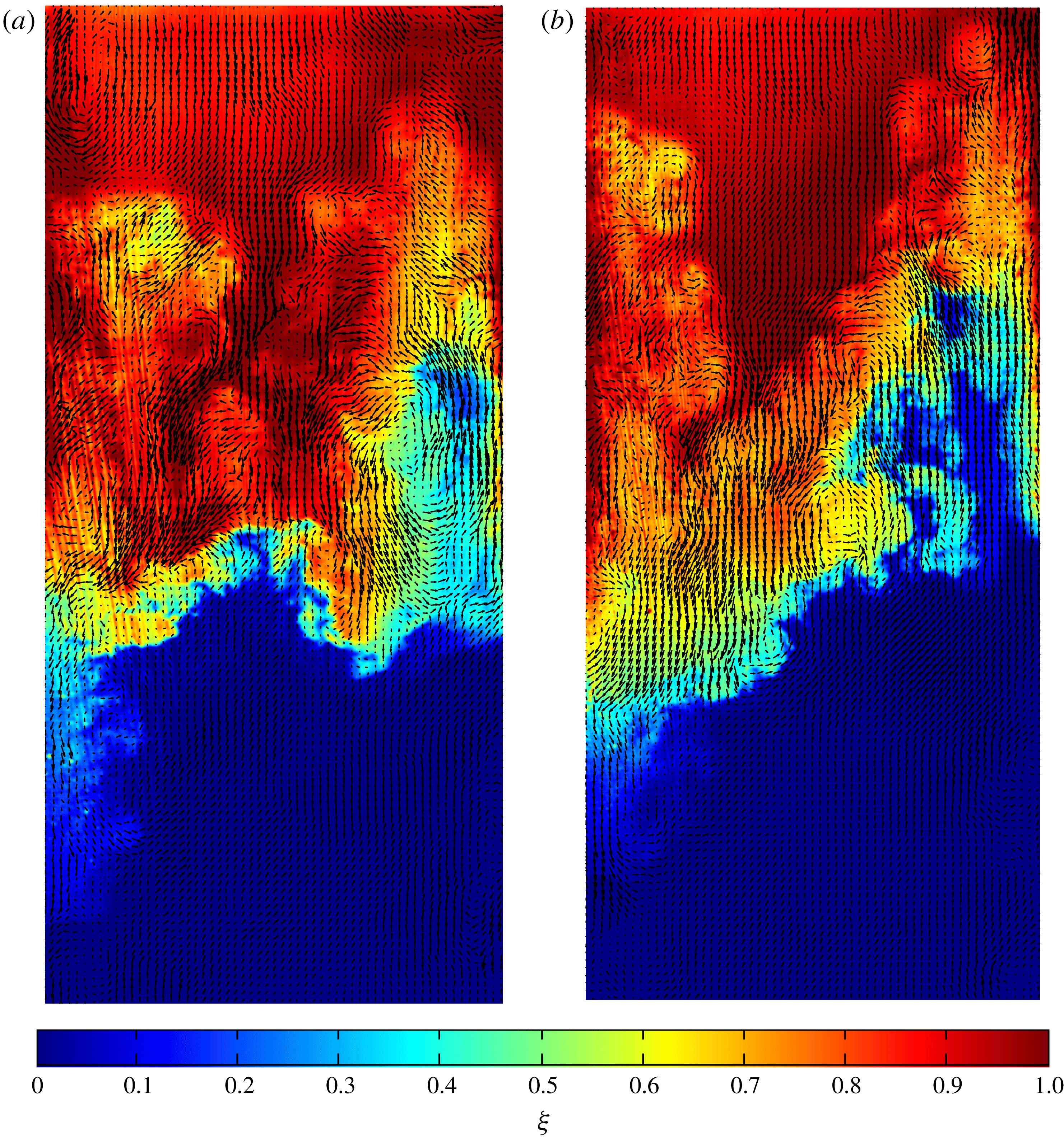
Reference Mohaghar, Carter, Musci, Reilly, McFarland and Ranjan2017). Figure 1 shows an example of registered PIV vectors with the corresponding PLIF field for both single- and multi-mode cases at the latest time after reshock for
 $M\sim 1.9$
, indicating the fidelity of the measurements made.
Simultaneous PLIF/PIV field showing velocity vectors over pseudocolour concentration (
 $\unicode[STIX]{x1D709}$
) fields at the latest time after reshock (
 $\unicode[STIX]{x1D70F}=4.35$
) at
 $M\sim 1.9$
, indicating several vortical structures in the flow, fidelity of measurements and accuracy of registry process. Only
 $1/5$
of calculated vectors shown for clarity. (a) Single-mode at latest time after reshock. (b) Multi-mode at latest time after reshock.
2.3 Experimental runs
The current experiments measure the evolution of the
 $\text{N}_{2}/\text{CO}_{2}$
interface inclined at
 $80^{\circ }$
with respect to the horizontal (
 $10^{\circ }$
mismatch between shock and interface). Two sets of measurements with an incident shock strength of Mach 1.9 are performed as part of the current experiments: an initial sweep of experimental times is done using only PLIF measurements to characterize the instability growth and the facility for both the single- (S) and multi-mode (M) interface conditions, which is followed by more detailed (and large ensemble) measurement sets using simultaneous PIV and PLIF at two times corresponding to the evolution from incident shock (
 $t=2~\text{ms}$
and 3.75 ms) and two times corresponding to post reshock (
 $t=4.6~\text{ms}$
and 6 ms). Here
 $t$
corresponds to experimental time relative to initial shock–interface interaction. The method of non-dimensionalized time calculation was explained in Mohaghar et al. (Reference Mohaghar, Carter, Musci, Reilly, McFarland and Ranjan2017). Non-dimensional time after incident shock is
 $\unicode[STIX]{x1D70F}_{i}=k{\dot{h}}_{0}t$
, and after reshock is computed using
 $\unicode[STIX]{x1D70F}_{r}=k\dot{h^{\prime }}_{0}t^{\prime }$
where
 $\dot{h^{\prime }}_{0}$
and
 $t^{\prime }$
are initial mixing-width growth rate and experimental time after reshock, respectively. In the current work, in order to have a continuous non-dimensional time (
 $\unicode[STIX]{x1D70F}$
),
 $\unicode[STIX]{x1D70F}_{r}$
(non-dimensional time after reshock) is added to the latest
 $\unicode[STIX]{x1D70F}_{i}$
(non-dimensional time after incident shock). The latest non-dimensional time after incident shock (
 $\unicode[STIX]{x1D70F}_{i}$
) is approximately 2.4 for both low and high Mach numbers. Therefore,
 $\unicode[STIX]{x1D70F}=\unicode[STIX]{x1D70F}_{i}$
before reshock, and
 $\unicode[STIX]{x1D70F}=\unicode[STIX]{x1D70F}_{r}+2.4$
after reshock. Table 1 summarizes the list of experimental times and ensemble sizes used for the current work for single- and multi-mode initial conditions. The observations from the time swept evolution experiments and those from the more detailed experiments are discussed in §§ 3 and 4.
Summary of experiments.

2.4 Initial condition creation
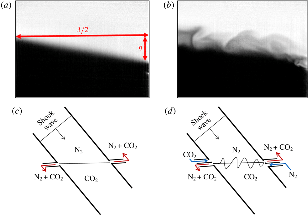
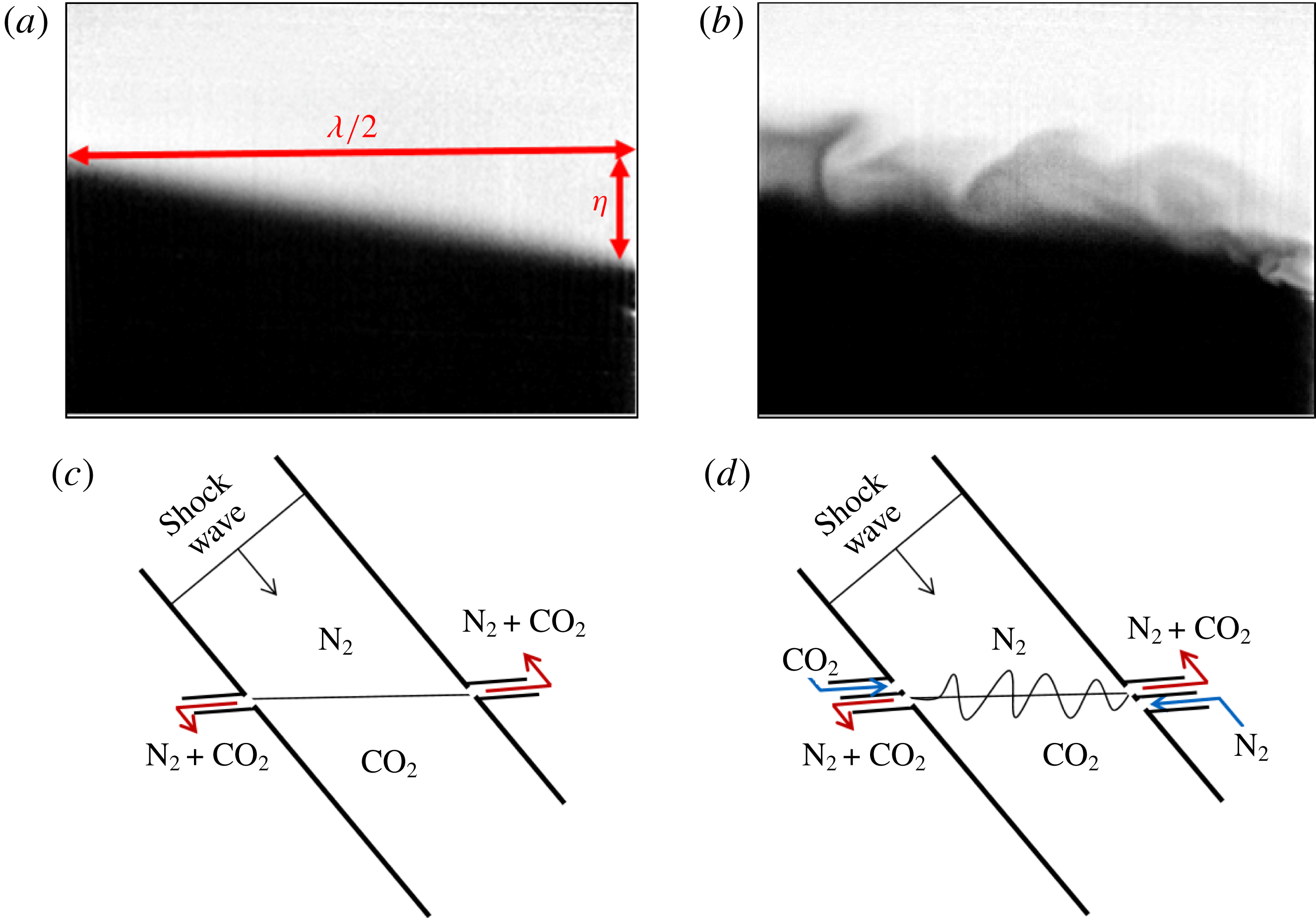
In order to create a consistent, slightly diffuse (less than 1 cm) interface, the light and heavy gases are injected from opposite sides of the driven section in a controlled manner at low mass flow rates – light gas through a port on the side wall just downstream of the diaphragm, and heavy gas from a port on the bottom end wall. Bleed slots on either side wall of the shock tube (aligned parallel to the ground) enable a stable free surface to be sustained between the light and heavy gases being injected. The inclined interface can be viewed as a half-wavelength of a sawtooth wave, and is henceforth referred to as the single-mode interface (S). Additionally, via a controlled cross-flow of the light and heavy gases, just below and above the interface, respectively, gentle shear between the two gases can be sustained along with buoyancy effects, leading to additional small-scale perturbations superposed on the predominantly single-mode interface due to Kelvin–Helmholtz and Rayleigh–Taylor instabilities. This interface is henceforth referred to as the multi-mode interface (M). The effects of these perturbations on RMI evolution are studied in this paper at
 $M\sim 1.9$
and compared with results at similar non-dimensional times at
 $M\sim 1.55$
(Mohaghar et al.
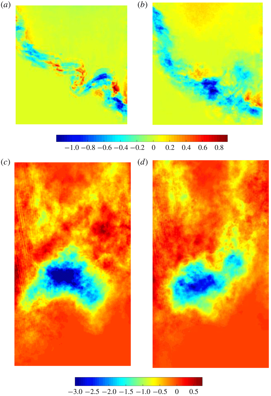
Reference Mohaghar, Carter, Musci, Reilly, McFarland and Ranjan2017). Figure 2 shows an example single-mode interface (where the cross-flow is turned off) and the multi-mode interface (where shear and buoyancy perturbs the interface). In both cases, the main feature is the inclination by
 $10^{\circ }$
with the incident shock, with the smaller perturbations superposed in the latter case. The initial condition characterization – the statistical description, the range of scales involved and the modal energy content of the density fluctuations in the multi-mode interface – was previously discussed by Mohaghar et al. (Reference Mohaghar, Carter, Musci, Reilly, McFarland and Ranjan2017).
Single- and multi-mode initial condition creation: (a,b) sample corrected single- and multi-mode initial condition images where nitrogen is light and carbon dioxide is dark. (c,d) Simplified schematic showing the general method of interface creation by outflowing the mixture of gases at the interface, shown as red arrows, and flowing pure nitrogen and carbon dioxide below and above the interface respectively (blue arrows) to create shear and buoyancy effects. In the schematic, the angle of the interface is slightly exaggerated for clarity. In both depictions gravity acts normal to the interface. The actual inlets and outlets consist of small perforations to prevent disturbance of the shock. (a) Sample single-mode initial condition. (b) Sample multi-mode initial condition. (c) Schematic of single-mode initial condition creation. (d) Schematic of multi-mode initial condition creation.
3 Analysis of flow development
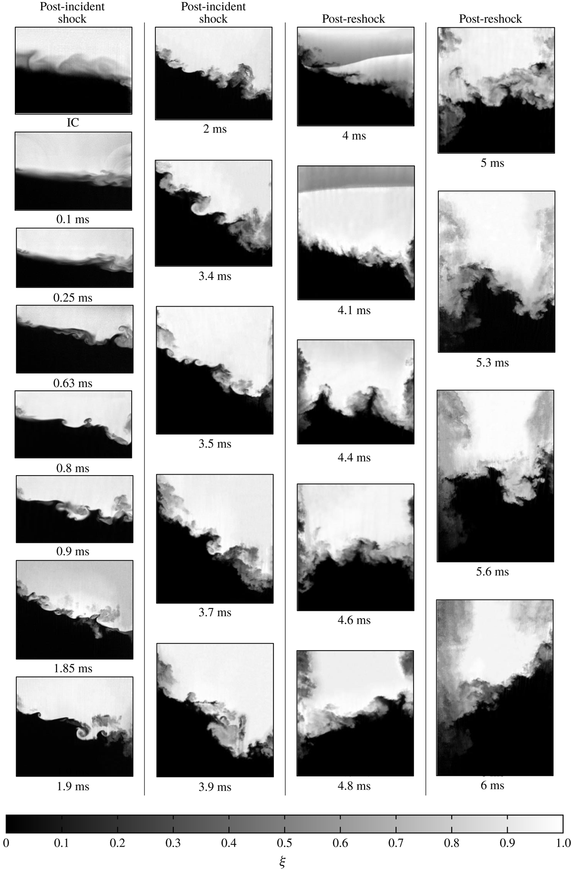
To understand the unique morphology of the RMI resulting from a particular set of parameters, the evolutions of the concentration fields are analysed to identify the interface mechanics through its development. This evolution for single and multi-mode cases at high Mach (
 $M\sim 1.9$
) is shown in figures 3 and 4. In the single-mode case (figure 3), the compression of the interface by the incident shock can be observed in the range
 $0<t<0.1~\text{ms}$
, which results in intensification of the scalar gradient across the interface. Few other developments are noticeable at the earliest times. A subtle, nearly sinusoidal waveform can be observed at
 $t=0.9~\text{ms}$
at a wavelength approximately equal to the width of the tube. After this time, the overall growth of the interface amplitude and further intensification resulting from its stretching are noticeable. Additional features with shorter wavelengths develop, some of which eventually grow to significant amplitudes. More importantly, the complex topology of the interface is evident with two well-developed roll-up features in the range
 $3.7~\text{ms}<t<3.9~\text{ms}$
, the late times before reshock. This forms the initial condition for reshock.
Concentration (
 $\unicode[STIX]{x1D709}$
) field evolution of single-mode initial condition at
 $M\sim 1.9$
with experimental times shown. Reshock arrives at the interface at
 $t\approx 4~\text{ms}$
(
 $\unicode[STIX]{x1D70F}\approx 2.4$
).

The main difference between the two Mach numbers (the current work at
 $M\sim 1.9$
and Mohaghar et al. (Reference Mohaghar, Carter, Musci, Reilly, McFarland and Ranjan2017)) at
 $M\sim 1.55$
before reshock, is the interface features at late times that are especially apparent in the single-mode case. While both the low and high Mach interfaces are fairly smooth and organized, the high Mach number case contains additional small perturbations and a complete roll-up feature which is visually evident in the single-mode case. These features are largely due to the tendency of vorticity along the surface to concentrate and roll up via the Kelvin–Helmholtz instability. These differences will also be discussed quantitatively in § 3.5.
At
 $t=4~\text{ms}$
the shock has been reflected off the bottom wall of the tube (reshock) and is travelling upwards, appearing as a sharp gradient in the PLIF image. The shock has been shaped by the interface and is beginning to replanarize at this time. The interface is compressed by reshock (as with the initial shock), and some small-amplitude, short-wavelength features can clearly be observed immediately after its traversal. As the long-wavelength perturbation undergoes a phase inversion, the additional features are also observed to invert, although their signature is much more subtle. Between images at 3.9 and 4.8 ms, the interface inverts, and the uppermost extent of heavy fluid before reshock becomes the lowest extent of light fluid. Additionally the two prominent roll-up features, where the heavy fluid penetrates into the light fluid before reshock, are inverted and are observed as two regions of light fluid penetrating into heavy fluid after reshock. After 4.8 ms these features become indistinguishable, and the interface begins to look increasingly chaotic. As the phase inversion at the long wavelength continues, a breakdown of scales and consequent increase in mixed material is observed.
A similar sequence showing the RMI evolution resulting from the multi-mode initial condition is presented in figure 4. Before reshock, the multi-mode case shows additional small-scale features throughout the evolution that were previously not seen with the single-mode interface. These observations are anticipated, owing to the greater modal content in the initial condition, and are similar to those observed in the low Mach number case (Mohaghar et al. Reference Mohaghar, Carter, Musci, Reilly, McFarland and Ranjan2017). Also, due to a larger modal content in the features present in the multi-mode case at late times before reshock, the interface seems to have fewer large-scale features immediately after reshock. This phenomenon is due to increased interaction of features which have different-signed vorticity, leading to a greater breakdown of coherent medium-sized features.
Concentration (
 $\unicode[STIX]{x1D709}$
) field evolution of multi-mode initial condition at
 $M\sim 1.9$
with experimental times shown. Reshock arrives at the interface at
 $t\approx 4~\text{ms}$
(
 $\unicode[STIX]{x1D70F}\approx 2.4$
).

3.1 Mixing width, mixed-mass thickness and mixed mass
With a qualitative understanding of the evolution of the single- and multi-mode interfaces, the quantitative aspects of the same using mixing width, mixed-mass thickness and mixed mass are discussed here. Mixing width (
 $h$
) is defined as the
 $5{-}95\,\%$
extent (in the shock propagation direction) of spanwise-averaged nitrogen volume fraction (Olson & Jacobs Reference Olson and Jacobs2009; Weber et al.
Reference Weber, Haehn, Oakley, Rothamer and Bonazza2012), and is a measure of the amplitude, or largest length scale, of the instability. The growth of the mixing width is dependent on the velocity jump of the interface (proportional to the Mach number of the initial shock/reshock).
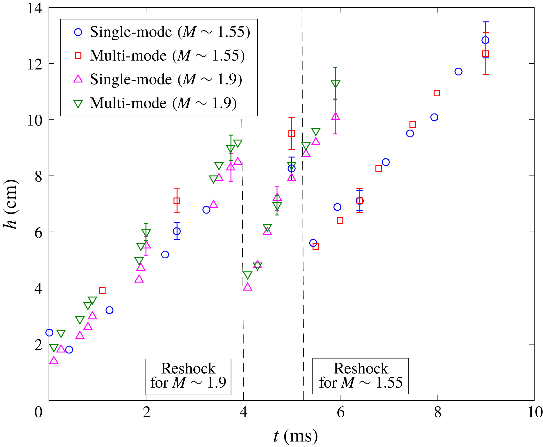
Figure 5 shows the evolution of the mixing width from the current experiments at
 $M\sim 1.9$
, alongside the
 $M\sim 1.55$
experiments of Mohaghar et al. (Reference Mohaghar, Carter, Musci, Reilly, McFarland and Ranjan2017) for both initial condition configurations. The dependence of the mixing width growth on the Mach number is evident, as explained before, with the slope of the
 $M\sim 1.9$
mixing width consistently higher than the
 $M\sim 1.55$
cases before and after reshock. The single- and multi-mode interfaces, however, show identical growth behaviour in the mixing width. This independence of the smaller modal content is anticipated as the growth in
 $h$
is predominantly driven by the largest mode of the initial perturbation (inclined interface in both the interfaces). The error bars indicate the statistical error which was computed based on standard deviation from the total number of experiments at each time where a large ensemble of simultaneous PLIF/PIV data were collected.
Comparison of overall mixing width (amplitude
 $h$
) of the interface after incident shock and after reshock for single and multi-mode initial conditions at both
 $M\sim 1.55$
and
 $M\sim 1.9$
. Error bars indicate the statistical error at times that larger ensembles of simultaneous PLIF/PIV data were collected. Data without error bars are from single experiments.
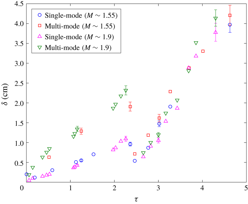
At any time, the mixing width only denotes the extent of the instability, and not the modal content or the scalar mixing. An additional length scale, termed the ‘mixed-mass thickness (
 $\unicode[STIX]{x1D6FF}$
)’, is defined in order to highlight the mixing dynamics below the large scale in the flow and to emphasize the effect of the initial condition. This definition considers the average streamwise thickness of the mixed material in the range
 $4Y_{N_{2}}Y_{CO_{2}}>0.84$
. This value is chosen based on the mass fraction range from 30 to 70 % light gas in order to consider highly mixed material. Here,
 $Y_{N_{2}}$
and
 $Y_{CO_{2}}$
are the mole fractions of light and heavy gases at each spanwise location, and
 $\unicode[STIX]{x1D6FF}$
is calculated as
 $$\begin{eqnarray}\unicode[STIX]{x1D6FF}=\frac{\displaystyle \int \int 4Y_{N_{2}}Y_{CO_{2}}\,\text{d}x\,\text{d}y}{\displaystyle \int \text{d}y}.\end{eqnarray}$$
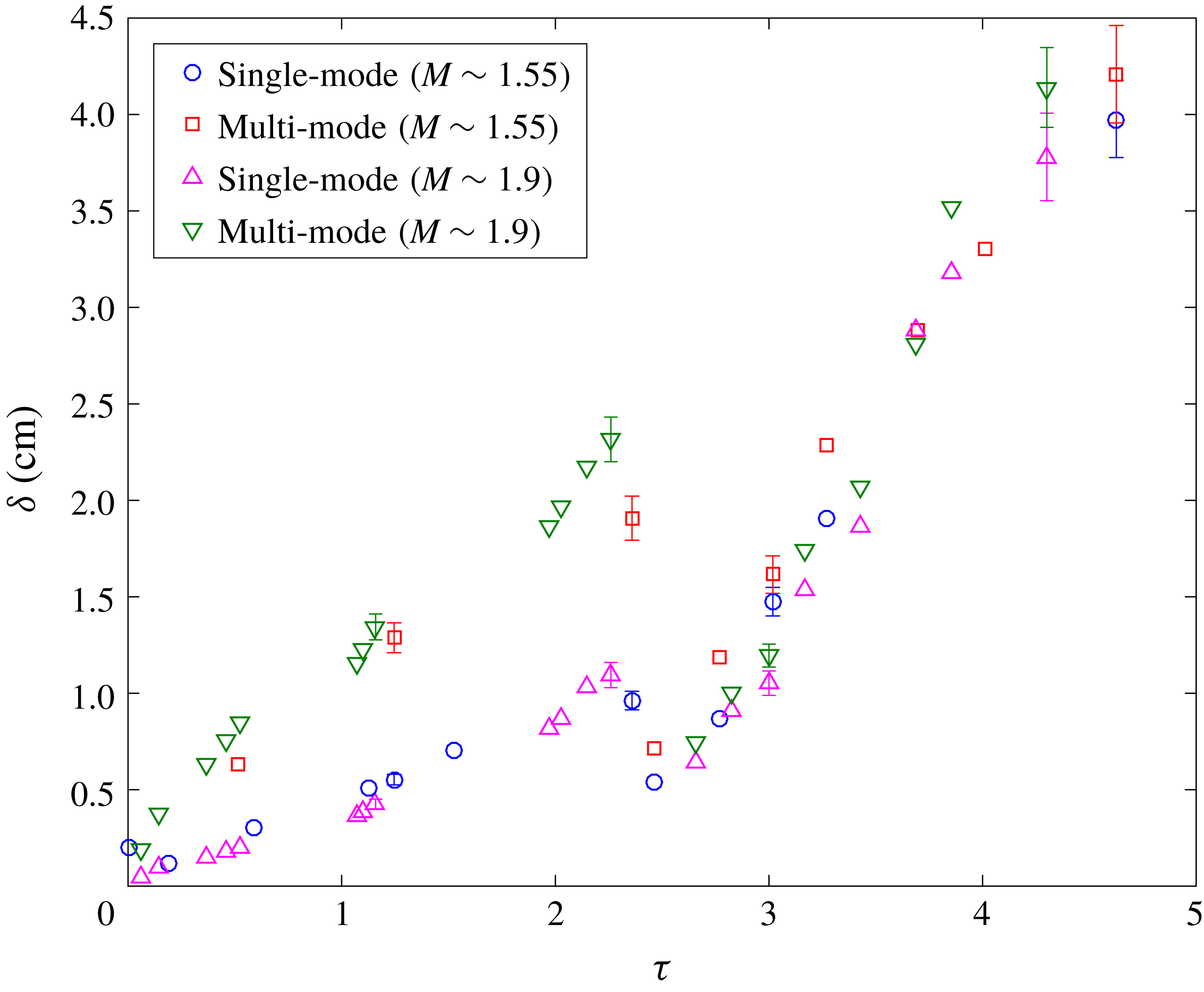
Figure 6 shows the evolution of
 $\unicode[STIX]{x1D6FF}$
, but with non-dimensionalized time instead. It must be noted that the multi-mode interface starts with a higher initial
 $\unicode[STIX]{x1D6FF}$
than the single-mode interface. As expected from the observations in figure 4, the
 $\unicode[STIX]{x1D6FF}$
of the multi-mode interface consistently grows faster than the single-mode case before reshock at both Mach numbers. Further, the
 $M\sim 1.9$
case has a slightly higher mixed-mass thickness than the
 $M\sim 1.55$
case, owing to the stronger growth and mixing in the former. After reshock, this quantity is not sensitive to the additional modal content of the multi-mode interface, largely due to the interface compression from reshock, as all the cases continue to evolve similarly to each other. Mixed-mass thickness is also used in § 4 for the investigation of mixing transition, as this is considered by the authors to be a more accurate indicator of the mixing dynamics in the flow than the mixing width.
Evolution of integral mixed-mass thickness (
 $\unicode[STIX]{x1D6FF}$
) in non-dimensional time,
 $\unicode[STIX]{x1D70F}$
for all cases.
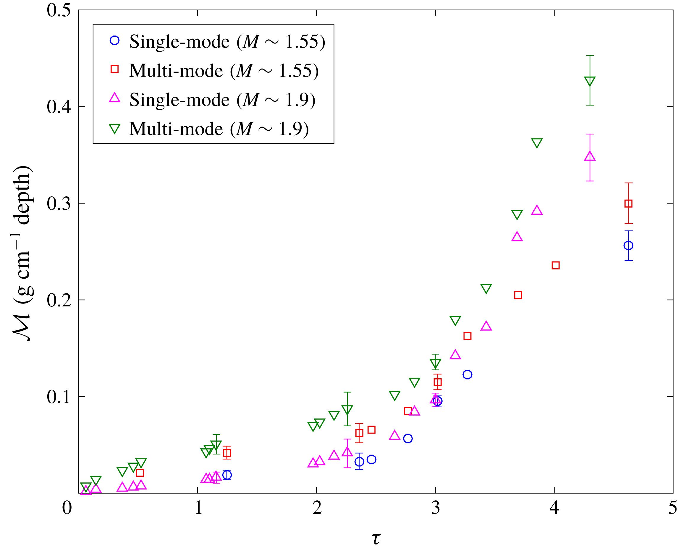
Mixed mass, which is a measure of how much mixed product exists in the flow, further quantifies the actual mixing of the gases at each evolution time investigated. The calculation of mixed mass assumes that material is distributed uniformly at sub-pixel scales. An important feature of this quantity is that it is monotonically increasing, and unlike mixing width and mixed-mass thickness, does not decrease with passage of reshock (Zhou, Cabot & Thornber Reference Zhou, Cabot and Thornber2016; Zhou Reference Zhou2017b
). Also, the mixed-mass calculation does not include the entrained, but unmixed, fluid. The mixed mass (
 ${\mathcal{M}}$
) is calculated as
 $$\begin{eqnarray}{\mathcal{M}}=\int 4\unicode[STIX]{x1D70C}Y_{N_{2}}Y_{CO_{2}}\,\text{d}V.\end{eqnarray}$$
Mixed mass is shown at various non-dimensional times in figure 7. A linear trend is observed for all cases before reshock, and, similar to mixed-mass thickness, the multi-mode case has a higher growth rate of mixed mass compared to the single-mode case. The single- and multi-mode cases at high Mach have slightly higher mixed mass compared to low Mach number cases before reshock at the same non-dimensional times. Post-reshock, however, unlike the trends in mixed-mass thickness, mixed mass is noticeably higher for the
 $M\sim 1.9$
case, due to the larger density jump, particularly with reshock. The ratio of the density after reshock to the one before reshock on average in the high Mach number case is 2.3 whereas this ratio is 1.8 in the low Mach number case. Also, the ratio of density in the high Mach number case to the low Mach number case is close to 1.3 and 1.6 before and after reshock, respectively. These higher values of density magnitude and higher increase in density magnitude due to reshock in the high Mach case lead to higher values and growth rate in mixed mass especially after reshock for the
 $M\sim 1.9$
case. This observation (of similar mixed-mass thickness but higher mixed mass in the post-reshock
 $M\sim 1.9$
cases) implies that the rate of entrainment is similar between the two Mach numbers, while the rate of molecular mixing is higher in the high Mach number case. This mixing paradigm will be further explored in the following section.
Evolution of integral mixed mass (
 ${\mathcal{M}}$
) in non-dimensional time,
 $\unicode[STIX]{x1D70F}$
for all cases.
3.2 Mixedness
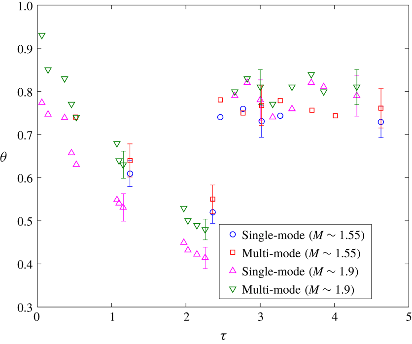
To compute the fraction of entrained material that is molecularly mixed, the mixedness,
 $\unicode[STIX]{x1D703}$
is calculated as
 $$\begin{eqnarray}\unicode[STIX]{x1D703}=\frac{\displaystyle \int \overline{X(1-X)}\,\text{d}x}{\displaystyle \int \overline{X}\,\overline{(1-X)}\,\text{d}x},\end{eqnarray}$$
where heavy fluid has a mole fraction of
 $$\begin{eqnarray}X=\frac{\unicode[STIX]{x1D70C}-\unicode[STIX]{x1D70C}_{1}}{\unicode[STIX]{x1D70C}_{2}-\unicode[STIX]{x1D70C}_{1}}.\end{eqnarray}$$
The evolution of this average mixedness in the mixed region at various nondimensional times is shown in figure 8. The average mixedness initially decreases after the initial shock passage due to the stretching of the interface and the high rate of entrainment as the two fluids undergo penetration within each other. Before reshock, the difference in mixedness between single-mode and multi-mode interfaces is more pronounced at higher Mach number. Further, due to a higher amount of entrained (but unmixed) fluid, the mixedness is observed to be lower for the high Mach number case than the low Mach number case, despite a higher amount of mixed material in the former. Similar behaviour was observed by Orlicz et al. (Reference Orlicz, Balasubramanian and Prestridge2013) in the gas curtain experiment at early times after incident shock. Weber et al. (Reference Weber, Haehn, Oakley, Rothamer and Bonazza2014) also observed similar behaviour for a higher Mach number at early times in a comparable metric to mixedness.
Contrarily, after reshock, higher mixedness is observed in the higher Mach number case; which is consistent with the aforementioned observations that the overall growth (mixing width) and mixed-mass thickness were similar between the two Mach numbers, but that the amount of mixed mass was higher in the high Mach number case after reshock. Mixedness is similar between the single- and multi-mode cases after reshock, as was also seen with
 $\unicode[STIX]{x1D6FF}$
in figure 6.
Evolution of integral mixedness (
 $\unicode[STIX]{x1D703}$
) in non-dimensional time,
 $\unicode[STIX]{x1D70F}$
for all cases.
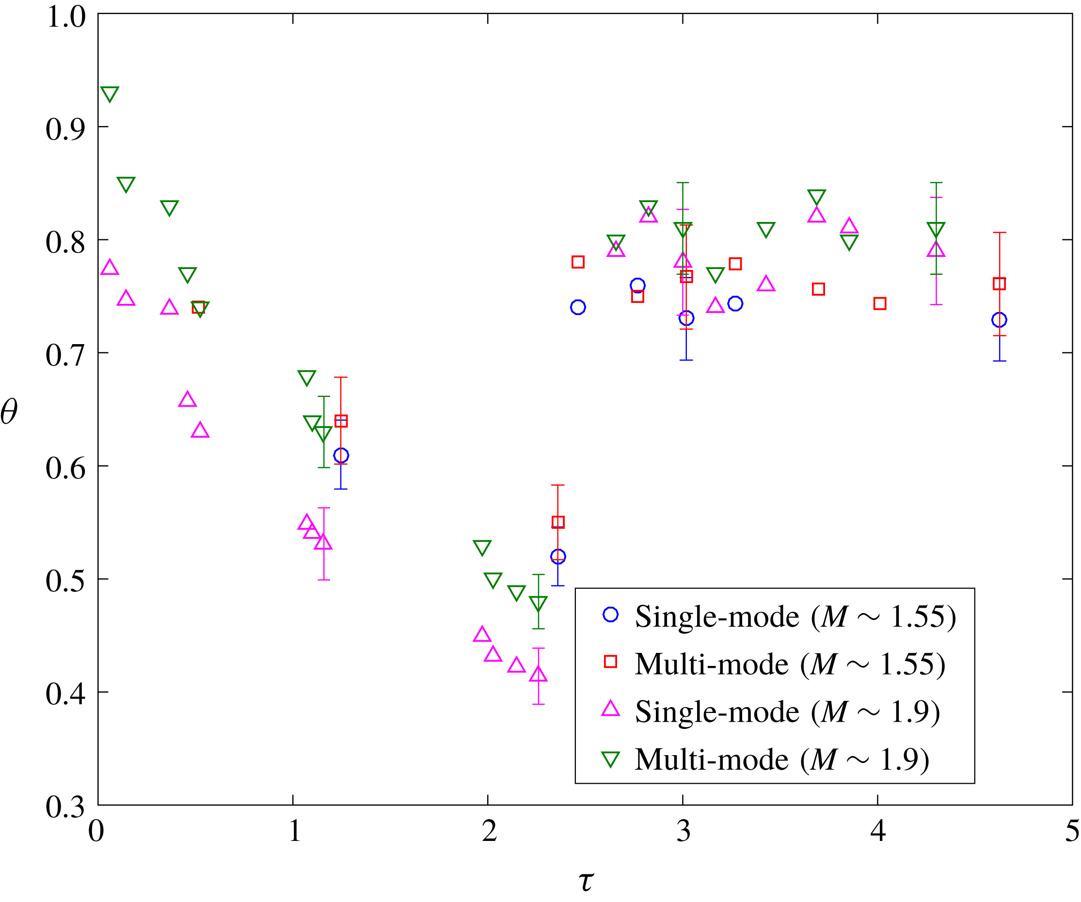
There has been much discussion of how the entrainment (due to pure fluid entering the mixing zone on either end) and molecular mixing rates might balance as the interface approaches a nonlinear state. Asymptotic values at late times have been proposed. In the current work, the interface at late times after reshock is beginning to display nonlinear behaviour and the value of mixedness is fairly constant. The late time value of mixedness for low Mach number is
 $0.76\pm 0.04$
and for high Mach number is
 $0.82\pm 0.04$
. Zhou et al. (Reference Zhou, Cabot and Thornber2016) found an asymptotic value (
 ${\sim}0.8$
) for similar Atwood and Mach numbers, and Tritschler et al. (Reference Tritschler, Olson, Lele, Hickel, Hu and Adams2014) found a similar asymptote value of 0.85 for
 $M=1.5$
and higher Atwood number, which are in reasonable agreement with the current work. Orlicz et al. (Reference Orlicz, Balasubramanian and Prestridge2013) observed that the average asymptotic value increases with increasing Mach number, consistent with the findings of the current work. However, the final value was found to be
 $0.94-0.97$
for the different Mach numbers which can be due to the gas curtain experiments having two interfaces unlike the current interface.
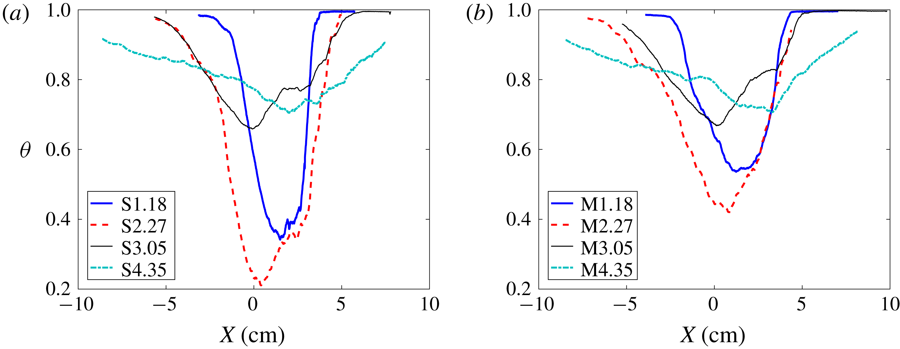
To investigate the effect of initial condition, it is useful to examine the profile of the spanwise average of mixedness at various streamwise locations along the mixing region. Figure 9 shows this at two times before and two times after reshock for the
 $M\sim 1.9$
cases investigated in the current work. While the overall trend is similar between the two interfaces, the multi-mode case shows much higher mixedness before reshock. Additionally, the spike side (
 $x<0$
, upward) is more mixed after reshock while entrainment is outpacing molecular mixing on the bubble side (
 $x>0$
, downward).
Effect of initial condition on temporal evolution of mixedness (
 $\unicode[STIX]{x1D703}$
) profiles in the streamwise direction before and after reshock at
 $M\sim 1.9$
for the (a) single-mode (S) and (b) multi-mode (M) cases.
 $X$
is distance from centre of mass.
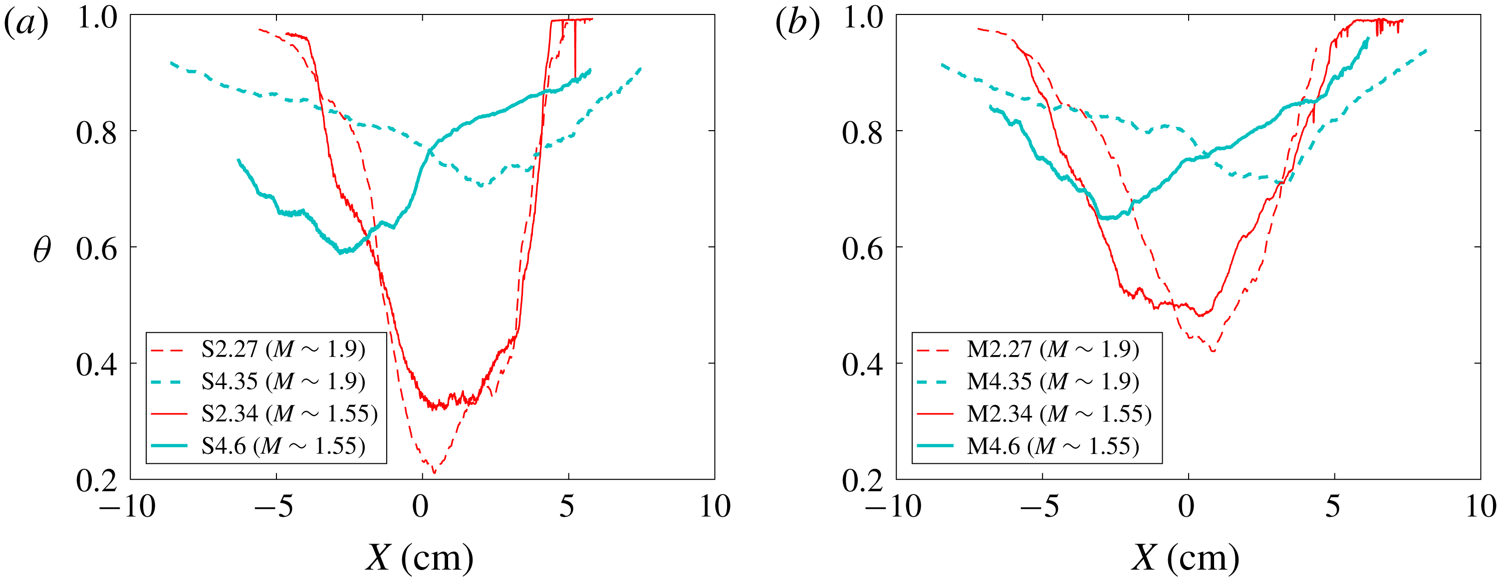
The effect of Mach number on the mixedness can be seen in figure 10. Before reshock, although the overall trend is similar, mixedness in the higher Mach number case is slightly lower than the lower Mach number case as was seen in the integral measurement in figure 9. After reshock there is a significantly higher amount of entrained and mixed fluid in the spike region (
 $x<0$
) of the high Mach number case for both single- and multi-mode conditions. This trend is reversed, however, in the
 $M\sim 1.55$
case where the bubble region (
 $x>0$
) shows higher
 $\unicode[STIX]{x1D703}$
. This behaviour is due to higher penetration of the spike into the core of the flow and subsequent breakdown of scales in the higher Mach number case, where the core of the flow is more mixed. Regarding the effect of Mach number on mixedness for different initial conditions, the spatial distribution of the mixedness is not changed by the additional perturbations of the multi-mode initial condition, but the magnitude is still noticeably larger before reshock and slightly larger after reshock for the multi-mode case. This suggests that the effects of Mach number and initial condition on this measurement could be independent of each other.
Effect of Mach number on temporal evolution of mixedness profiles in the streamwise direction before and after reshock at for (a) single-mode (S) and (b) multi-mode (M) cases.
 $X$
is distance from centre of mass.
3.3 Density self-correlation
The density-specific volume correlation, also referred to as the density self-correlation (DSC), is the correlation between density fluctuations and specific volume fluctuations (
 $b=-\langle \unicode[STIX]{x1D70C}^{\prime }(1/\unicode[STIX]{x1D70C})^{\prime }\rangle$
). This is an important statistic in the closure of many turbulence models, and is typically termed the
 $b$
parameter in Besnard et al. (Reference Besnard, Harlow, Rauenzahn and Zemach1992), or the BHR model. The parameter has been thoroughly investigated in previous studies such as Balakumar et al. (Reference Balakumar, Orlicz, Ristorcelli, Balasubramanian, Prestridge and Tomkins2012) and Mohaghar et al. (Reference Mohaghar, Carter, Musci, Reilly, McFarland and Ranjan2017). These works can be referred to for a more thorough analysis of DSC and the effect of the averaging choice in computing the same. Particularly in spatially inhomogeneous flows, specific volume fluctuations computed via spatially averaged quantities show apparent increase in the DSC values, when compared with the fluctuations with respect to the ensemble average. Furthermore, the information about the spatial variance of density is already contained within mixedness (Livescu & Ristorcelli Reference Livescu and Ristorcelli2008), and the two variables embody similar information about the flow. Figure 11 highlights this similarity between trends of the profiles of mixedness and the DSC, when fluctuations are computed from spanwise-averaged quantities. It shows that for both single- and multi-mode cases after incident shock, the DSC increases as the interface stretches, causing sharpening in the gradient of density. After reshock, the flow evolves to a more homogeneously mixed state, which is indicated by the decrease in DSC with time after reshock.
Temporal evolution of density self-correlation profile (DSC, b) along the streamwise direction before and after reshock with fluctuations computed from spanwise-averaging method at
 $M\sim 1.9$
for the (a) single-mode (S) case and (b) multi-mode (M) case.
 $X$
is distance from centre of mass.
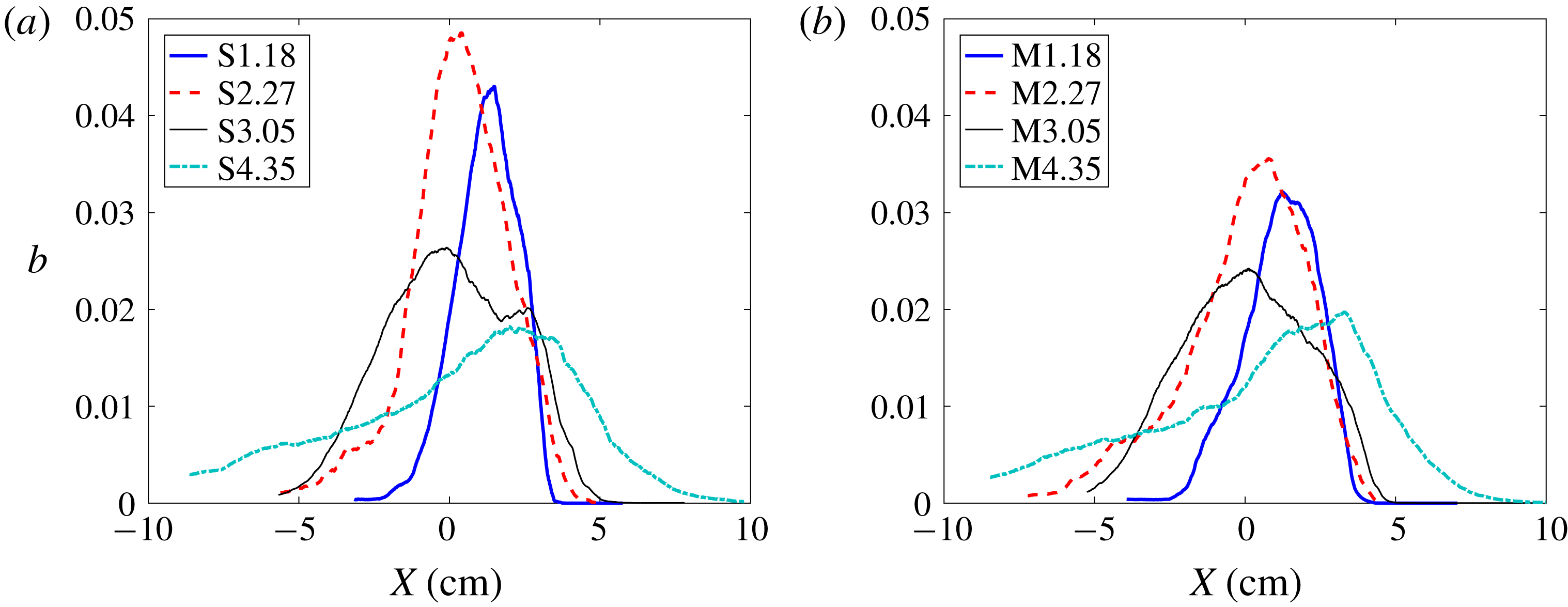
Similar to previous work (Mohaghar et al.
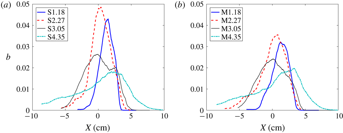
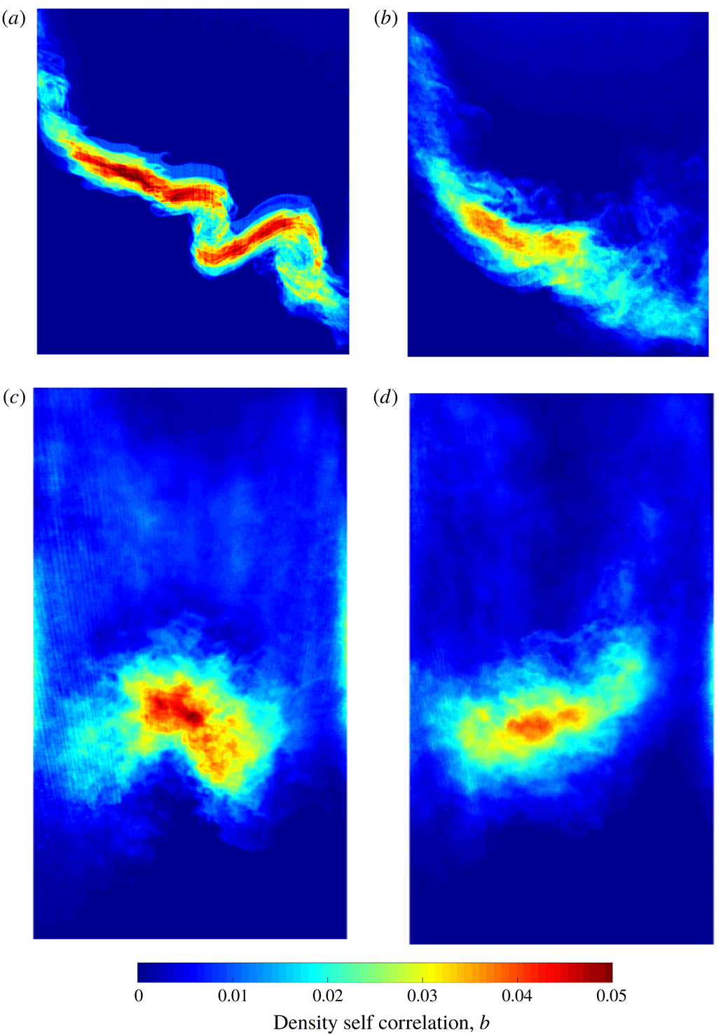
Reference Mohaghar, Carter, Musci, Reilly, McFarland and Ranjan2017), the DSC is also calculated from the ensemble-averaging method of calculating fluctuations. In this method, the DSC represents the mixing which is occurring in the flow, whereas mixedness indicates the portion of entrained fluid which has already mixed. This method results in a DSC field, which can then be spanwise averaged to yield a profile. Figures 12 and 13 show the profiles and ensemble-averaged fields, respectively, of the DSC, with this method. The similarity between the single-mode and multi-mode cases is evident. A double peak at
 $\unicode[STIX]{x1D70F}=2.27$
(late time before reshock) can be seen in the single-mode case and corresponds to the more organized structures in the spatial field. A slightly larger tail is also seen at
 $\unicode[STIX]{x1D70F}=4.3$
(late time after reshock) in the single-mode case due to a secondary spike that commonly occurs at the centre of the field. As a result of the variability in the multi-mode case, this tail is slightly smaller. Although the intensity observed in the fields is similar before and after reshock, the peak of the DSC profile increases after reshock because the active mixing region on the bubble side is oriented parallel to the spanwise direction.
Effect of initial condition on temporal evolution of the density self-correlation profile (DSC, b) along the streamwise direction before and after reshock where fluctuations are computed from the ensemble-averaging method at
 $M\sim 1.9$
for the (a) single-mode (S) case and (b) multi-mode (M) case.
 $X$
is distance from centre of mass.

Figure 13 shows the DSC fields from which the profiles in figure 12 are calculated. The value of this visualization method is emphasized, by first noting that although the spanwise average of the DSC is nearly identical between the single-mode and multi-mode cases, the fields show striking differences in structures spatially. The variability of the multi-mode case results in larger areas of more diffuse fluctuation intensity, while the consistency of the single-mode case yields small, concentrated regions where fluctuations display greater variance in the ensemble. This is true before and after reshock.
Fields of density self-correlation before (a,b) and after reshock (c,d) at
 $M\sim 1.9$
for the (a,c) single-mode (S) case and (b,d) multi-mode (M) case.

For a clearer comparison between Mach numbers, figure 14 shows just one time before reshock and one time after reshock of the
 $M\sim 1.55$
and
 $M\sim 1.9$
cases. There is a significantly greater DSC for the high Mach number case before and after reshock, and there is a reversal in the side of the flow that contains the most mixing. This observation and trend reversal were also seen in the mixedness profiles after reshock in figure 8. Furthermore, the difference between the single- and multi-mode cases is not very striking for the
 $M\sim 1.9$
case. The low Mach number case is also very similar after reshock. Before reshock, however, there is a significant difference where the single-mode interface has three peaks which are much more distinct. Overall, the increase in Mach number increases the mixing before and after reshock, and smears regions of intense mixing before reshock.
Effect of Mach number on temporal evolution of density self-correlation profile along the streamwise direction before and after reshock computed from ensemble-averaging method for the (a) single-mode (S) case and (b) multi-mode (M) case.
 $X$
is distance from centre of mass.

In addition to the DSC itself, analysis of each term of the DSC budget can yield insights into the mechanisms that are affecting the local rate of change of the variable (Tomkins et al. Reference Tomkins, Balakumar, Orlicz, Prestridge and Ristorcelli2013). The following is one form of the evolution equation (Besnard et al. Reference Besnard, Harlow, Rauenzahn and Zemach1992), which shows this relationship and numerically identifies each term of interest.
 $$\begin{eqnarray}\displaystyle \frac{\unicode[STIX]{x2202}b}{\unicode[STIX]{x2202}t}+\widetilde{U}_{j}b_{,j}[1] & = & \displaystyle 2a_{j}b_{,j}[2]-2a_{j}(1+b)\frac{\overline{\unicode[STIX]{x1D70C}}_{,j}}{\overline{\unicode[STIX]{x1D70C}}}[3]+\overline{\unicode[STIX]{x1D70C}}\left(\frac{\langle u_{j}^{\prime }\unicode[STIX]{x1D70C}^{\prime }(1/\unicode[STIX]{x1D70C})^{\prime }\rangle }{\overline{\unicode[STIX]{x1D70C}}}\right)_{,j}[4]\nonumber\\ \displaystyle & & \displaystyle +\,2\overline{\unicode[STIX]{x1D70C}}\langle (1/\unicode[STIX]{x1D70C})^{\prime }\unicode[STIX]{x1D735}\boldsymbol{\cdot }u^{\prime }\rangle [5].\end{eqnarray}$$
The numbers in square brackets (
 $[1-5]$
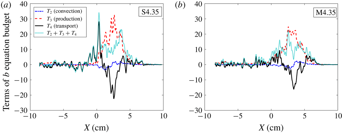
) refer to various terms in the equation. Of particular interest are terms 2 through 4, since term-1 is advection and term-5 is negligible compared to the others. The individual terms were first measured experimentally by Tomkins et al. (Reference Tomkins, Balakumar, Orlicz, Prestridge and Ristorcelli2013), where the fluctuations were calculated from the spanwise-averaging method to compare with simulations. Contrarily, figure 15 shows the spanwise-averaged profiles of the field calculated from ensemble-averaged means for each term of interest
 $[2-4]$
at the latest time after reshock. The ensemble fields themselves are shown subsequently in figure 16. Comparing the two initial conditions, the single-mode case shows sharper profiles indicating greater gradients in certain areas of the flow, while the multi-mode case has smaller maxima and is more evenly distributed. Otherwise, the morphology of the profiles is similar between the two cases. Both cases have a peak in the sum of terms which closely represents the overall rate of change and additional local peaks throughout the mixing region. Terms 2 (convection) and 4 (transport) undergo changes in sign. The more relevant observation being that transport term changes from positive, to negative, and back to positive, generally, with small undulations. This is more obvious in the multi-mode case. This implies that the transport term increases the DSC near the edges of the mixed region and transports it from its centre. Term three shows that production is higher interior to the mixing region with a bias towards the bubble side (
 $x>0$
).
Comparison of the relative magnitudes of term 2 (convection), term 3 (production) and term 4 (transport) in the DSC evolution equation at the latest time after reshock (
 $\unicode[STIX]{x1D70F}=4.35$
) for both (a) single-mode and (b) multi-mode cases at
 $M\sim 1.9$
.

Figure 16 provides further details on the mechanics of the DSC. While the main observable differences in spanwise-averaged profiles between the single and multi-mode cases were in magnitude, the fields of DSC terms provide further illumination of physical behaviour of the flow. The fields in figure 16 highlight a difference in the shape of the spatial distribution more obviously. Also, the DSC term fields are observed to have slightly more intense regions and more variation in sign than was observable in the spanwise-averaged plots in which these features lead to lower values.
Comparison between fields of different terms in the DSC evolution equation at the latest time after reshock (
 $\unicode[STIX]{x1D70F}=4.35$
) for both (a) single-mode and (b) multi-mode cases at
 $M\sim 1.9$
.
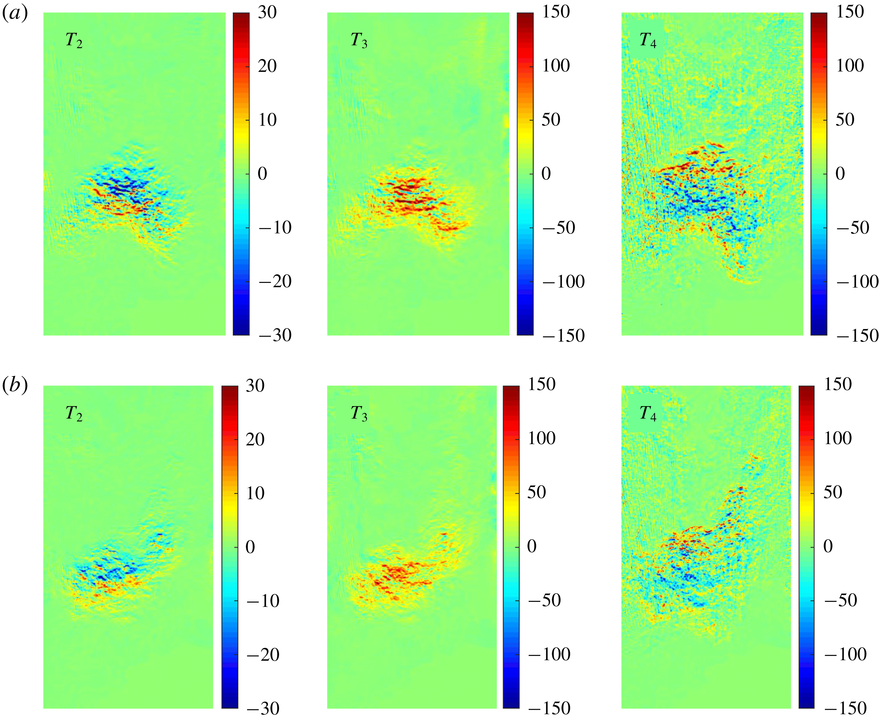
Between the single- and multi-mode cases, the consistently different morphology of the multi-mode interface is observable in all of the fields of these terms. All of the terms are slightly stronger in the single-mode case due to the higher level of consistency (low variance) of the interface shape, placing fluctuations in concentrated areas along the interface, while the multi-mode case terms are more diffuse due to higher variability/nonlinearity of the interface.
Regarding the relative contribution of each term to the total budget, term 2 (convection), which is characterized by turbulent mass flux,
 $a$
, is of much lower magnitude than the production and transport terms. This term is observed to decrease the DSC on the light gas side, but to increase it on the heavy gas side of the mixing region.
It is observed that production term 3, primarily affects the interior of the mixing region. This term is mostly positive in both cases; however, the single-mode case is larger and displays small pockets of negative production, which are likely to be damped out due to the more random interface of the multi-mode case. The transport term (term 4) is similar in magnitude to production, but the configuration of the two terms (3 and 4) is complementary; while the DSC is produced in the interior of the mixing region, it is transported out (negative values of term 4) of the centre of the mixing region to the edges. This finding should be considered in light of current discussion of the asymptotic value of mixedness, suggesting a connection between the mixing dynamics in the interior of the mixing region and the influx of pure fluid at the edges which propagates a balance between entrained and molecularly mixed fluid at late times.
3.4 Methods of velocity field decomposition
In general, fluctuations should be calculated from averages over homogeneous dimensions (average fluctuating quantities are invariant with that dimension). In many turbulent flows there may be multiple spatial dimensions, and possibly the temporal dimension, which provide this necessary homogeneity. Furthermore, in flows where there is dimensional dependence of a fluctuating quantity, averaging should not be performed over dimensions in which this inhomogeneity occurs. The RMI is temporally evolving, which precludes temporal averaging. Furthermore, in most RMI flows there is significant spatial inhomogeneity throughout the flow even after transition to turbulence. This spatial inhomogeneity can be due to the dependence on initial conditions, continued influx of pure fluid with a velocity preference at the edges of the mixing region, and conditional dependence (correlation) of velocity and density fluctuations. This spatial inhomogeneity can be seen, for example, in figure 13 for late times before and late times after reshock, where the fields of density self-correlation are clearly not homogeneous.
The comparison between ensemble and spanwise averaging, and the large difference between them were discussed in the previous work (Mohaghar et al.
Reference Mohaghar, Carter, Musci, Reilly, McFarland and Ranjan2017). Ensemble averaging in this work is identified by brackets (
 $\langle \bullet \rangle$
) whereas spatial averaging is indicated by an overbar (
 $\overline{\bullet }$
). In addition, a moving boxcar averaging method is used in the recent work by Reese et al. (Reference Reese, Ames, Noble, Oakley, Rothamer and Bonazza2018), where the spatial filter window size was chosen as
 $1/20$
of the average mixing height. To compare these two methods of averaging, relative velocity fluctuations (
 $u_{rel}^{\prime }$
) calculated using the boxcar averaging method are compared with velocity fluctuations from ensemble averaging (
 $u^{\prime }$
) at the latest time after reshock for a velocity field sample and are shown in figure 17. The velocity fluctuation for the ensemble-averaging method is defined as follows:
 $$\begin{eqnarray}\displaystyle & \displaystyle u_{b}=(\overline{u_{i}})_{x,y} & \displaystyle\end{eqnarray}$$
 $$\begin{eqnarray}\displaystyle & \displaystyle u_{rel}=u_{i}-u_{b} & \displaystyle\end{eqnarray}$$
 $$\begin{eqnarray}\displaystyle & \displaystyle u^{\prime }=u_{rel}-\langle u_{rel}\rangle , & \displaystyle\end{eqnarray}$$
while for the boxcar averaging method, it is calculated as
 $$\begin{eqnarray}u_{rel}^{\prime }=u_{rel}-(\overline{u_{rel}})_{boxcar},\end{eqnarray}$$
where the boxcar average is taken over the filter window.
Decomposition of a sample velocity field at the latest time after reshock: (a) velocity relative to the bulk flow, its ensemble average and its fluctuating component and (b) velocity relative to the bulk flow, its boxcar average and the difference between these two. The results are averaged in the spanwise direction for clarity.
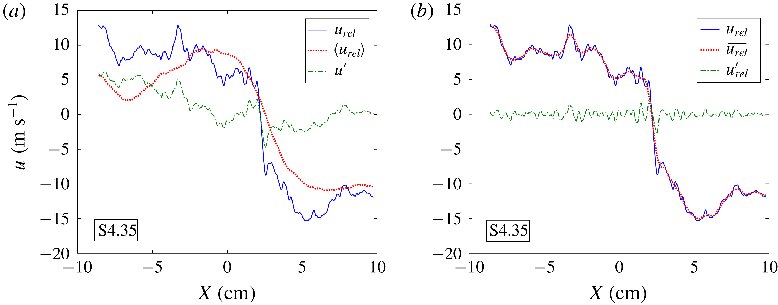
The comparison between ensemble and boxcar averaging (figure 17) shows that fluctuations from the boxcar averaging method indicate fine-scale features in each realization, based on local spatial variance rather than fluctuations from the ensemble dataset. Also, this method is very sensitive to the filter size. Therefore, in this work, consistent with the previous work (Mohaghar et al. Reference Mohaghar, Carter, Musci, Reilly, McFarland and Ranjan2017), fluctuations are calculated from ensemble averages, with the exception of calculations used to exemplify differences in the averaging methods.
3.5 Analysis of vortex sheet roll-ups in the single mode case
In this section, the effect of different shock strengths on the distribution of vortex roll-up features along the interface is investigated. This is an important topic, but has received limited attention thus far (Zabusky Reference Zabusky1999). The latest time before reshock for the single-mode interface at both Mach numbers was chosen to analyse the vorticity concentration and roll-up features. This case was chosen because the vortex roll-up features are repeatable and distinguishable.
In order to extract the location of the interface between the two gases, the gradient-based Canny edge detection method is applied to concentration fields. This method computes an approximate pixel by pixel gradient, and is thresholded locally or globally to distinguish steep gradients. This can be accomplished for the current work using a simple threshold (Canny Reference Canny1986). This method has been used widely in the combustion field for flame edge detection (Malm et al.
Reference Malm, Sparr, Hult and Kaminski2000; Sweeney & Hochgreb Reference Sweeney and Hochgreb2009; Slabaugh, Pratt & Lucht Reference Slabaugh, Pratt and Lucht2015; Reisenhofer, Kiefer & King Reference Reisenhofer, Kiefer and King2016; Fries et al.
Reference Fries, Ochs, Saha, Ranjan and Menon2019). Because there is a sharp gradient between the two fluids in the case shown, this method gives an accurate interface location. Additionally, to increase the accuracy of the measurement and reduce error, corrected PLIF images are pre-processed with a
 $3\times 3$
Gaussian filtering to reduce the effect of noise in the interface region. The vorticity fields are obtained by taking the discrete curl of two-dimensional velocity fields (Reilly et al.
Reference Reilly, McFarland, Mohaghar and Ranjan2015; Mohaghar et al.
Reference Mohaghar, Carter, Musci, Reilly, McFarland and Ranjan2017). Finally, to characterize and compare localized vorticity and roll-up locations, vorticity concentration fields are registered with the interface locations identified using edge detection. The results are shown in figure 18.
The figure shows concentration fields (left) and interface edges superimposed over vorticity fields (right) for the single-mode case at the latest time before reshock for (a)
 $M\sim 1.55$
and (b)
 $M\sim 1.9$
, respectively. Also shown are streamwise averages of (c) vorticity profiles and (d) interface crossings (from canny edge detection) for these two cases.

The interface crosses any streamwise line (vertical in figure 18) multiple times at any roll-up location. Therefore, roll-up locations are identified by calculating the total length of interface crossings (
 $N_{crossings}\ast \text{d}x$
) at each streamwise line. This is ensemble averaged and shown along the spanwise direction in figure 18(c). Furthermore, to analyse regions of vorticity localized within the roll-ups, the vorticity fields are averaged in the streamwise direction (
 $X$
) similarly, and shown in figure 18(d). It is observed that there is a strong correlation between the peaks of the interface crossings and vorticity concentration, which indicates that regions of vorticity concentration coincide with roll-up locations.
Comparison between high and low Mach numbers suggests that there are 3 large and 3 small roll-ups and peaks in vorticity concentration in the high Mach number case whereas there are 1 large and 2 small roll-ups and vorticity peaks in the low Mach number case. Finally, the total interface length is computed and averaged over the ensemble. The ratios of this quantity to ensemble average of mixing width for each case are also calculated, which are
 $39.72/8.56=4.64$
for high Mach (
 $M\sim 1.9$
) compared to
 $24.12/8.26=2.92$
for
 $M\sim 1.55$
. Overall, comparison of the number of roll-ups and arc-length to mixing-width ratio indicates that the high Mach number results in greater vorticity deposition which leads to more roll-ups (higher secondary perturbation wavenumber) and consequently more stretching of the interface.
4 Mixing transition analysis
4.1 Turbulent mass flux, Reynolds stress and anisotropy analysis
The turbulent mass-flux velocity,
 $a(x,y)_{i}=\langle \unicode[STIX]{x1D70C}^{\prime }u_{i}^{\prime }\rangle /\langle \unicode[STIX]{x1D70C}\rangle$
is closely related to the
 $b$
parameter (density self-correlation), since
 $b$
appears in the production of turbulent mass flux. Additionally, turbulent mass flux appears in the primary production term of turbulent kinetic energy (Livescu & Ristorcelli Reference Livescu and Ristorcelli2008; Tomkins et al.
Reference Tomkins, Balakumar, Orlicz, Prestridge and Ristorcelli2013). It also appears in the second term of the Reynolds stress decomposition. The averaging performed over the ensemble yields one field of turbulent mass flux for each case at each time. Then, to obtain a profile, these fields are averaged in the spanwise direction similar to the presentation of
 $b$
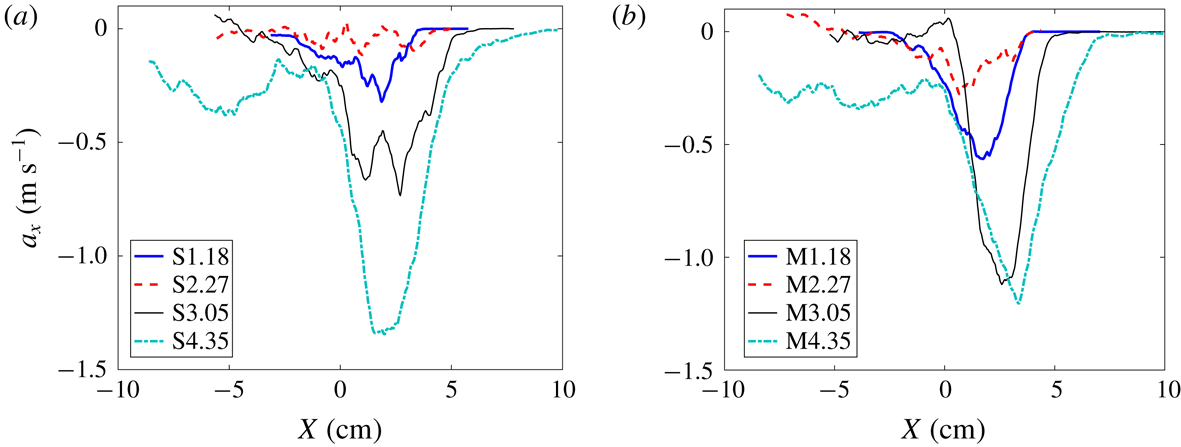
fields and profiles. Since the streamwise component of velocity fluctuation is dominant in this flow, the streamwise mass-flux velocity is shown here. The results for fields are shown for the high Mach number case in figure 20 in addition to spanwise-averaged profiles (figure 19) to have a better understanding of the physics of the flow.
Effect of initial condition on temporal evolution of turbulent mass-flux (
 $a_{x}$
) profiles along the streamwise direction before and after reshock at
 $M\sim 1.9$
for the (a) single-mode (S) case and (b) multi-mode (M) case.

The turbulent mass flux indicates intense penetration of the gases within each other driven by turbulent fluctuations. Where lighter than average fluid moves with higher than average velocity (causing negative density fluctuations coupled with a positive streamwise velocity fluctuation), this leads to a negative turbulent mass flux. On average, this phenomenon is seen throughout most of the flow. An interesting feature that can be identified in the mass-flux fields before reshock is the location of roll-up features, especially in the single-mode case where there are alternating positive and negative turbulent mass-flux regions due to the cresting motion of the roll-ups. In the location of a roll-up, the heavy gas tends to penetrate upward (negative direction) and the light gas tends to push downward near the top of the roll-up. However, on the crest and interior of the roll-up, heavy gas tends to move down and light gas moves upward resulting in regions of positive mass-flux velocity. In the multi-mode case, since the fluctuations are distributed over a larger portion of the flow, and there is more mixed material, this behaviour in turbulent mass flux is less evident than in the single-mode case. After reshock, similar to the density self-correlation fields, density and velocity fluctuations are more concentrated in one part of the flow in the single-mode case, compared to the more diffuse distribution of fluctuations along the interface in the multi-mode case due to higher variability or nonlinearity of the initial interface perturbation.
Fields of turbulent mass flux (
 $a_{x}$
) before (a,b) and after reshock (c,d) at
 $M\sim 1.9$
for the (a,c) single-mode (S) case and (b,d) multi-mode (M) case.

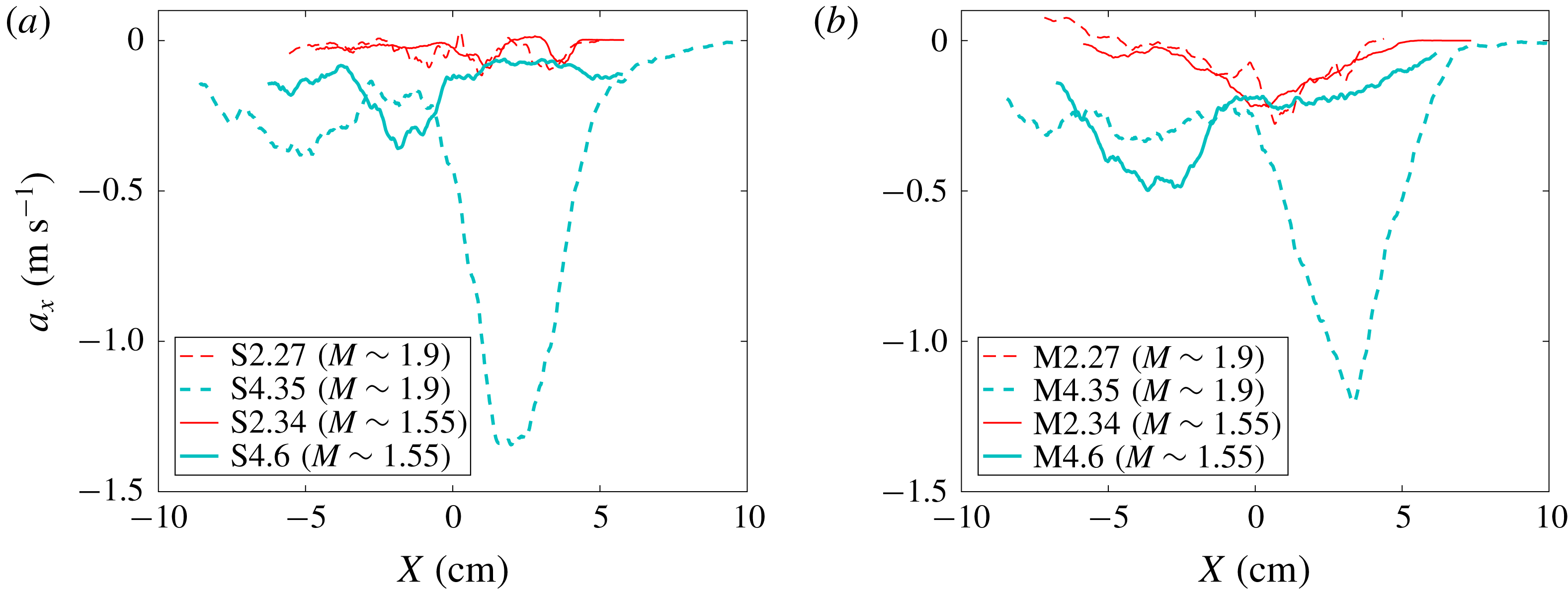
These interesting features are concealed in spanwise-averaged profiles, especially before reshock, in this inhomogeneous flow. However, the relative magnitude of turbulent mass flux between low and high Mach number cases can be observed in the spanwise-averaged profiles in figure 21. The magnitude of turbulent mass flux after reshock is almost three times higher than the low Mach number case. Moreover, similar to density self-correlation profiles, the peak of turbulent mass flux is shifted to the bubble side in the high Mach number case compared to the low Mach number case where this occurs on the spike side. This indicates that active mixing and greater production of turbulent kinetic energy is occurring on the bubble side for the high Mach number case. This phenomenon occurs in the flow due to higher fluctuations in the streamwise direction and therefore higher penetration of heavy gas to the core of the flow on the spike side which creates more mixed material on that side in the high Mach number case.
Mach number comparison on the temporal evolution of turbulent mass-flux (
 $a_{x}$
) profiles along the streamwise direction before and after reshock at both
 $M\sim 1.55$
and
 $M\sim 1.9$
for the (a) single-mode (S) case and (b) multi-mode (M) case.
Another measure related to turbulence intensity and transport is the Favre-averaged Reynolds stress. The components of the Reynolds stress, including the aforementioned term containing mass flux, are given by:
 $$\begin{eqnarray}\unicode[STIX]{x1D619}_{ij}=\langle \unicode[STIX]{x1D70C}u_{i}^{\prime \prime }u_{j}^{\prime \prime }\rangle =\langle \unicode[STIX]{x1D70C}\rangle \langle u_{i}^{\prime }u_{j}^{\prime }\rangle -\langle \unicode[STIX]{x1D70C}\rangle \langle a_{i}\rangle \langle a_{j}\rangle +\langle \unicode[STIX]{x1D70C}^{\prime }u_{i}^{\prime }u_{j}^{\prime }\rangle ,\end{eqnarray}$$
where the double prime indicates Favre averaging (
 $u_{i}^{\prime \prime }=u_{i}-\langle \unicode[STIX]{x1D70C}u_{i}\rangle /\langle \unicode[STIX]{x1D70C}\rangle$
). The streamwise profile of relative contribution of the three terms in the Reynolds stress for
 $\unicode[STIX]{x1D619}_{11}$
is shown in figure 22 for both single and multi-mode cases at
 $M\sim 1.9$
before and after reshock. The first term, which is the mean density times the velocity fluctuation correlation, is clearly the dominant contributor at each time for both cases. A similar trend was observed for the components,
 $\unicode[STIX]{x1D619}_{11},\unicode[STIX]{x1D619}_{12}$
and
 $\unicode[STIX]{x1D619}_{22}$
, of the Reynolds stress tensor. The turbulent mass-flux term (
 $T_{2}$
) is at least 1000 times smaller than the first term. The third term, which is the triple correlation term, is approximately 10 times larger than the second term and 100 times smaller than the first term. This finding indicates the importance of the contribution of the first term to the Reynolds stress and its significance for modelling, which was also observed by Balakumar et al. (Reference Balakumar, Orlicz, Ristorcelli, Balasubramanian, Prestridge and Tomkins2012) and Shankar & Lele (Reference Shankar and Lele2014) at higher Atwood number. In addition, the spanwise average of these terms highlights that the main differences for different initial conditions before and after reshock occur in the second term (turbulent mass-flux term). The ratio of the second term to the first term for the multi-mode case before reshock is uniformly distributed, and slightly larger compared to the single-mode case, which is due to uniform distribution of density–velocity fluctuations along the interface in the multi-mode case whereas there are concentrated fluctuations in the roll-up locations in the single-mode case due to coherent structures and less mixing (figure 23
a). The reshock effect on the mass-flux term is shown in figure 23(b). After reshock,
 $T_{2}/\unicode[STIX]{x1D619}_{11}$
increases significantly, which is expected due to higher velocity and density fluctuations. However, even if the ratio is almost 10–100 times larger than this ratio before reshock, the contribution of the mass-flux term is still less than 0.01 of the first term’s contribution.
Relative contribution of three terms in the Reynolds stress equation before (a,b) and after reshock (c,d) for (a,c) single-mode and (b,d) multi-mode cases at
 $M\sim 1.9$
.

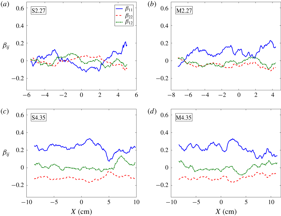
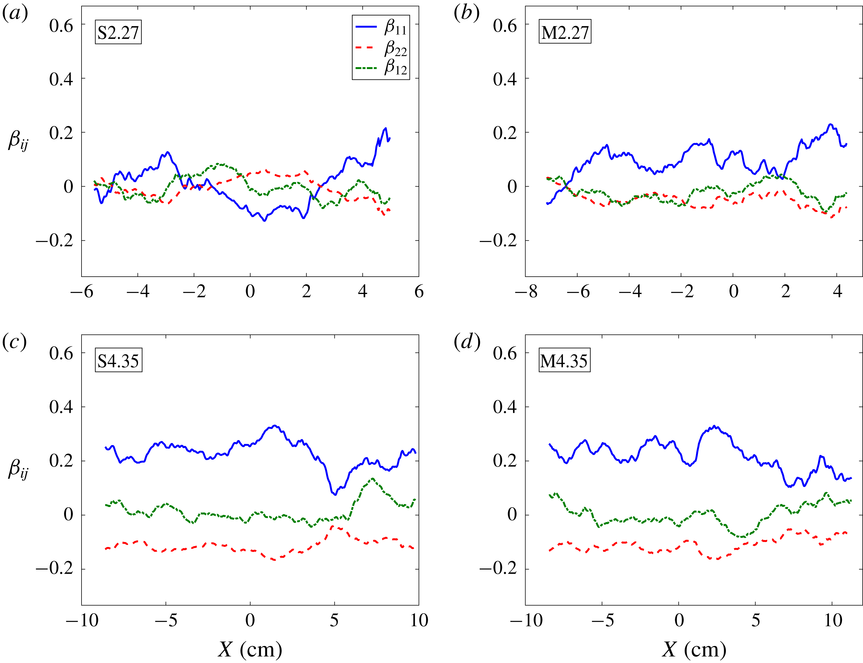
Another important parameter related to Reynolds stress is anisotropy. The normalized anisotropy is defined as
 $$\begin{eqnarray}\unicode[STIX]{x1D6FD}_{ij}=\frac{\unicode[STIX]{x1D619}_{ij}}{\unicode[STIX]{x1D619}_{kk}}-\frac{1}{3}\unicode[STIX]{x1D6FF}_{ij}.\end{eqnarray}$$
Anisotropy has been discussed previously for the low Mach number case (Mohaghar et al.
Reference Mohaghar, Carter, Musci, Reilly, McFarland and Ranjan2017). The normalized anisotropy has a limited range:
 $\unicode[STIX]{x1D6FD}_{kk}=-1/3$
,
 $\unicode[STIX]{x1D6FD}_{kk}=+2/3$
and
 $\unicode[STIX]{x1D6FD}_{kk}=0$
; corresponding to zero turbulent kinetic energy in the
 $k$
-direction, all turbulent kinetic energy in that direction and the isotropic turbulence limit, respectively. Additionally, the magnitude of the anisotropy tensor,
 $\Vert \unicode[STIX]{x1D737}\Vert =\unicode[STIX]{x1D6FD}_{ij}\unicode[STIX]{x1D6FD}_{ij}$
at each time is important to understand the physical reason for the variations in scaling of the turbulent kinetic energy spectra. Similar to the analysis of anisotropy in Mohaghar et al. (Reference Mohaghar, Carter, Musci, Reilly, McFarland and Ranjan2017), since only the streamwise and spanwise components of velocity are available, the velocity fluctuations in the out-of-plane direction is assumed to be equal to those of the spanwise direction.
Effect of (a) initial condition and (b) reshock on the contribution of the second component of Reynolds stress. (a) Contribution of mass flux term for single- and multi-mode cases at latest time before reshock. (b) Contribution of mass flux term for multi-mode cases before and after reshock.

The spanwise average of the normalized anisotropy tensor for the high Mach number case for both initial conditions is plotted in figure 24. In addition, to investigate the effect of Mach number on anisotropy, the spanwise average of the magnitude of the anisotropy tensor for both Mach numbers is shown in figure 25. After incident shock, at the latest time before reshock, the anisotropy magnitude in the high Mach number case for the single-mode case is less than the low Mach number case, specifically close to the centre of mass, which is due to transfer of energy from streamwise to spanwise direction in the two large roll-up locations, but this difference is not significant. However, in the multi-mode case before reshock, and noticeably after reshock, the anisotropy is significantly higher in the high Mach number case. This large difference is due to higher turbulent kinetic energy in the flow, especially in the streamwise component, because of the stronger incident shock and reshock. As a result of this higher energy in the shock direction, more time is needed for the flow to transfer energy from the shock-direction component to the spanwise and out-of-plane components to reduce anisotropy. High anisotropy is particularly noticeable in the high Mach number case on the bubble side (light gas side), since the flow is still strongly inhomogeneous and active mixing is occurring in that region for both initial conditions. Overall, before reshock at high Mach, similar to the low Mach number case, turbulent kinetic energy in the flow at some regions near the centre of mass is transferred from the shock direction toward the spanwise direction and there is localized isotropy in the flow. However, after reshock in the higher Mach number case, there is a strong anisotropy in the flow and energy in the streamwise direction is dominant. Even at late time after reshock, Tritschler et al. (Reference Tritschler, Olson, Lele, Hickel, Hu and Adams2014) observed that the anisotropy reached a small asymptotic value, but did not reach zero.
Normalized anisotropy tensor components before (a,b) and after (c,d) reshock for both (a,c) single-mode and (b,d) multi-mode cases at
 $M\sim 1.9$
.
Effect of Mach number on the magnitude of the normalized anisotropy tensor along the streamwise direction before and after reshock at both
 $M\sim 1.55$
and
 $M\sim 1.9$
for the (a) single-mode (S) case and (b) multi-mode (M) case.

4.2 Turbulent length scales, Reynolds number and energy spectra
Using simultaneous PLIF/PIV measurements, it is possible to compute different length scales to study mixing transition. Taylor microscales and integral scales can be calculated from velocity fluctuations (Pope Reference Pope2000). The integral scale is calculated from the longitudinal spatial covariance of velocity fluctuations using
 $$\begin{eqnarray}L_{i}=\int f(r)\,\text{d}r,\end{eqnarray}$$
where
 $f(r)$
is the velocity autocorrelation function defined as
 $$\begin{eqnarray}f(r)=\frac{\langle u_{i}^{\prime }(x)u_{i}^{\prime }(x+r)\rangle }{\langle (u_{i}^{\prime })^{2}\rangle }.\end{eqnarray}$$
The Taylor microscale then can be calculated from the curvature of the autocorrelation function (Champagne, Harris & Corrsin Reference Champagne, Harris and Corrsin1970; Ramaprabhu & Andrews Reference Ramaprabhu and Andrews2004; Weber et al. Reference Weber, Haehn, Oakley, Rothamer and Bonazza2014; Mohaghar et al. Reference Mohaghar, Carter, Musci, Reilly, McFarland and Ranjan2017; Reese et al. Reference Reese, Ames, Noble, Oakley, Rothamer and Bonazza2018),
 $$\begin{eqnarray}\unicode[STIX]{x1D706}_{T}=\left[-\frac{1}{2}\frac{\text{d}^{2}f(0)}{\text{d}r^{2}}\right]^{-1/2}.\end{eqnarray}$$
By fitting a quadratic function to the central three points of the autocorrelation of streamwise and spanwise velocity fluctuations, Taylor microscales in the streamwise (
 $\unicode[STIX]{x1D706}_{T,u^{\prime }}$
) and spanwise (
 $\unicode[STIX]{x1D706}_{T,v^{\prime }}$
) directions, respectively, can be computed. The combined Taylor microscale from the autocorrelation function is obtained by
 $\unicode[STIX]{x1D706}_{T,corr}=$
 $\sqrt{\unicode[STIX]{x1D706}_{T,u^{\prime }}^{2}+\unicode[STIX]{x1D706}_{T,v^{\prime }}^{2}}$
. To increase the reliability of results, the Taylor microscale is also calculated using the variance and gradient of velocity fluctuations (Pope Reference Pope2000),
 $$\begin{eqnarray}\unicode[STIX]{x1D706}_{T,u_{i}}=\sqrt{\frac{2\langle u_{i}^{\prime ^{2}}\rangle }{\langle (\unicode[STIX]{x2202}u_{i}^{\prime }/\unicode[STIX]{x2202}x_{i})^{2}\rangle }}.\end{eqnarray}$$
It was shown that the order of magnitude from the two methods is similar (Mohaghar et al.
Reference Mohaghar, Carter, Musci, Reilly, McFarland and Ranjan2017). The combined Taylor microscale from the gradient method is found by
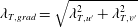 $\unicode[STIX]{x1D706}_{T,grad}=\sqrt{\unicode[STIX]{x1D706}_{T,u^{\prime }}^{2}+\unicode[STIX]{x1D706}_{T,v^{\prime }}^{2}}$
, similar to the combined Taylor microscale calculated from the correlation function. Finally, the total Taylor microscale is measured by averaging the results from the correlation and gradient methods,
 $\unicode[STIX]{x1D706}_{T}=(\unicode[STIX]{x1D706}_{T,grad}+\unicode[STIX]{x1D706}_{T,corr})/2$
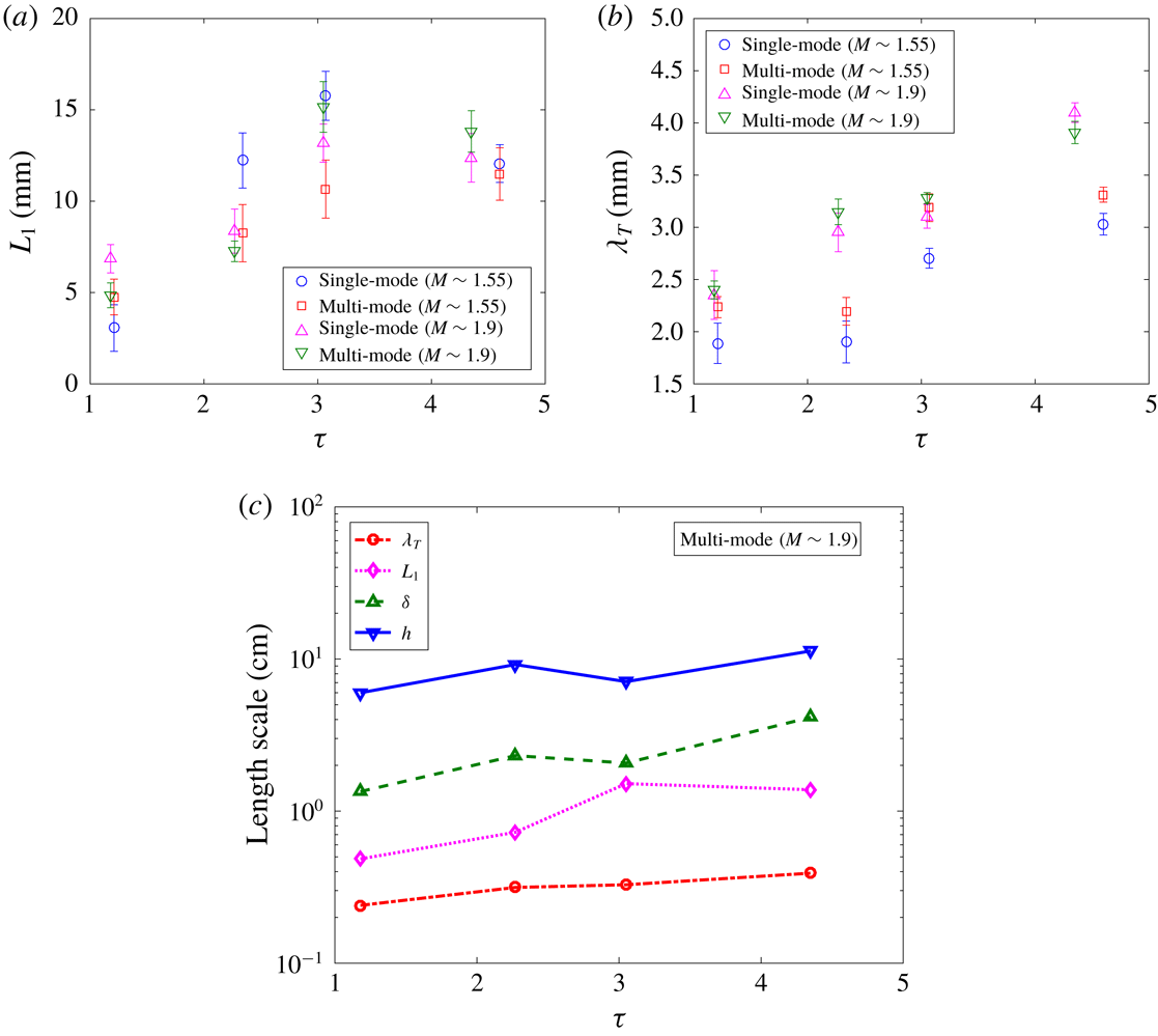
. The time evolution of the integral scale and Taylor microscale for both single- and multi-mode cases and at both Mach numbers are plotted in figure 26(a,b). The magnitude of the integral scale is not affected by Mach number, and similar values are obtained for both Mach numbers at each time. Although the trend in the Taylor microscale is similar to that of
 $M\sim 1.55$
of (Mohaghar et al.
Reference Mohaghar, Carter, Musci, Reilly, McFarland and Ranjan2017), the magnitude of the
 $M\sim 1.9$
Taylor microscale is a factor of
 $1.25\pm 0.05$
times that of the former at similar non-dimensional times. This is due to stronger fluctuations in the current case. Additionally, a Reynolds number scaling which is found to have the best agreement with the velocity-based Taylor microscale in this particular flow is
 $\unicode[STIX]{x1D706}_{T}=18\unicode[STIX]{x1D6FF}Re^{-1/2}$
, whereas Orlicz et al. (Reference Orlicz, Balasubramanian, Vorobieff and Prestridge2015) found a scaling of
 $\unicode[STIX]{x1D706}_{T}=10\unicode[STIX]{x1D6FF}Re^{-1/2}$
in their gas curtain experiments. Finally, in order to get an overall picture of scale separation, the different length scales computed in the current work (from the largest scale, mixing width, computed in § 3.1 to the Taylor microscale) are plotted in figure 26 for the multi-mode case at higher Mach.
Temporal evolution of (a) integral scale (
 $L_{1}$
) at both Mach and initial conditions, (b) Taylor micro-scale (
 $\unicode[STIX]{x1D706}_{T}$
) at both Mach and initial conditions and (c) summary of length scales at
 $M\sim 1.9$
for multi-mode case.
 $\unicode[STIX]{x1D70F}$
is non-dimensional time.
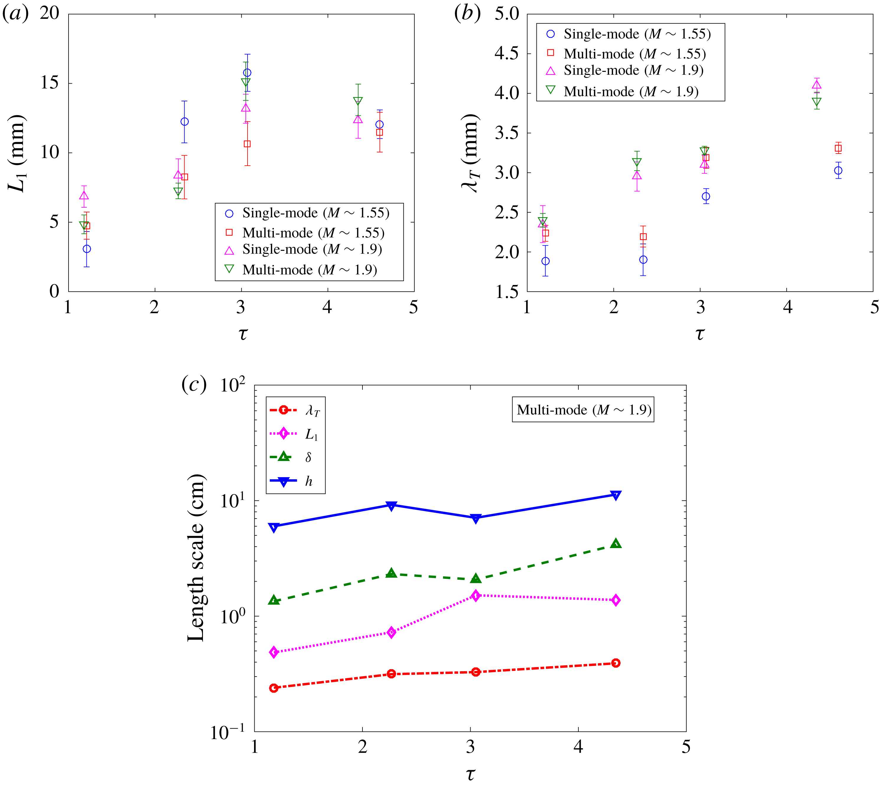
To evaluate mixing transition and inertial range formation, the ratio of Liepmann–Taylor (
 $\unicode[STIX]{x1D706}_{L}$
) to inner-viscous (
 $\unicode[STIX]{x1D706}_{\unicode[STIX]{x1D708}}$
) scales can be investigated, with the assumption that the flow will have an established inertial range if
 $\unicode[STIX]{x1D706}_{L}/\unicode[STIX]{x1D706}_{\unicode[STIX]{x1D708}}\gg 1$
(Lombardini et al.
Reference Lombardini, Pullin and Meiron2012). To evaluate this criterion and to determine whether mixing transition may have occurred in this particular flow (Dimotakis Reference Dimotakis2000), the ratio is calculated using
 $$\begin{eqnarray}\frac{\unicode[STIX]{x1D706}_{L}}{\unicode[STIX]{x1D706}_{\unicode[STIX]{x1D708}}}\approx \frac{5Re^{-1/2}\unicode[STIX]{x1D6FF}}{50Re^{-3/4}\unicode[STIX]{x1D6FF}}\approx \frac{1}{10}Re^{1/4}.\end{eqnarray}$$
This criterion is equivalent to
 $Re>10^{4}$
which is suggested by Dimotakis (Reference Dimotakis2000) for the onset of mixing transition. Therefore to investigate the satisfaction of mixing transition criteria (Dimotakis Reference Dimotakis2005) and the minimum state of Zhou (Reference Zhou2007), the local Reynolds number based on turbulent kinetic energy is calculated (Tomkins et al.
Reference Tomkins, Balakumar, Orlicz, Prestridge and Ristorcelli2013; Orlicz et al.
Reference Orlicz, Balasubramanian, Vorobieff and Prestridge2015) as
 $$\begin{eqnarray}Re=\frac{u_{rms}\unicode[STIX]{x1D6FF}}{\unicode[STIX]{x1D708}_{mix}},\end{eqnarray}$$
where
 $u_{rms}=\sqrt{\overline{u_{i}^{\prime ^{2}}}}$
,
 $\unicode[STIX]{x1D708}_{mix}$
is the kinematic viscosity of the mixture (details of calculation discussed in Mohaghar et al. (Reference Mohaghar, Carter, Musci, Reilly, McFarland and Ranjan2017)), and mixed-mass thickness is chosen for the length scale
 $\unicode[STIX]{x1D6FF}$
instead of mixing width (
 $h$
). Mixed-mass thickness is a more representative mixing length scale in this type of flow, analogous to the length scales chosen in other canonical flows, which were outlined by Dimotakis (Reference Dimotakis2005).
The kinematic viscosity before and after reshock are approximately
 $6.27\times 10^{-6}$
and
 $4.08\times 10^{-6}~\text{m}^{2}~\text{s}^{-1}$
at
 $M\sim 1.55$
, and
 $5.49\times 10^{-6}$
and
 $3.14\times 10^{-6}~\text{m}^{2}~\text{s}^{-1}$
at
 $M\sim 1.9$
, respectively. The local Reynolds number for both single and multi-mode cases at both Mach numbers is plotted in figure 27. The dashed lines represent the mixing transition criterion (
 $Re=1-2\times 10^{4}$
, Dimotakis (Reference Dimotakis2000)) and the dotted line indicates the minimum state criterion (
 $Re\approx 1.6\times 10^{5}$
, Zhou (Reference Zhou2007)). Before reshock at early times, the Reynolds numbers are below the transition criterion for all cases, but the multi-mode case has a significantly higher
 $Re$
than the single-mode case. At late time, although
 $Re$
increases for all cases, only the multi-mode case at higher Mach exceeds both criterion for mixing transition. After reshock, due to an impulse jump in turbulent kinetic energy, there is a rapid increase in
 $Re$
for all cases. Both single- and multi-mode cases have similar values for the two Mach numbers at early times after reshock, though the
 $M\sim 1.9$
 $Re$
increases at a faster rate due to the higher growth rate of mixed-mass thickness. The Reynolds number criterion for mixing transition is also satisfied at all times after reshock.
Reynolds number estimation with non-dimensional time (
 $\unicode[STIX]{x1D70F}$
) based on turbulent kinetic energy and mixed-mass thickness. Dashed lines indicate a threshold for turbulent mixing (Dimotakis Reference Dimotakis2000) and the dotted line indicates the minimum state criterion (
 $Re\approx 1.6\times 10^{5}$
, Zhou (Reference Zhou2007)).

In addition to the Reynolds number criterion, the other important criterion to consider for mixing transition is proposed by Robey et al. (Reference Robey, Zhou, Buckingham, Keiter, Remington and Drake2003) and Zhou, Robey & Buckingham (Reference Zhou, Robey and Buckingham2003), particularly for time-evolving flow like RMI flow. The new time-dependent scale which is proposed for the upper bound of the inertial range is
 $\unicode[STIX]{x1D706}_{D}=5\times (\unicode[STIX]{x1D708}t)^{1/2}$
. Robey et al. (Reference Robey, Zhou, Buckingham, Keiter, Remington and Drake2003) and Zhou et al. (Reference Zhou, Robey and Buckingham2003) suggested an extension to the mixing transition work of Dimotakis (Reference Dimotakis2000) when the Liepmann scale is strongly evolving with time. According to this criterion, the inertial range forms in the flow when the viscous diffusion scale (time-dependent critical scale) is larger than the inner-viscous scale (i.e.
 $\unicode[STIX]{x1D706}_{D}/\unicode[STIX]{x1D706}_{\unicode[STIX]{x1D708}}>1$
, where
 $\unicode[STIX]{x1D706}_{\unicode[STIX]{x1D708}}=50Re^{-3/4}\unicode[STIX]{x1D6FF}$
). The inner-viscous scales and the time-dependent scale at each time for both Mach numbers and both initial conditions are plotted in figure 28. The ratio
 $\unicode[STIX]{x1D706}_{D}/\unicode[STIX]{x1D706}_{\unicode[STIX]{x1D708}}$
is greater than one only at the latest time after reshock, and is close to one at the latest time before reshock for the higher Mach number cases and early time after reshock for both Mach numbers. Therefore, unlike the Reynolds number criterion, the latest time after reshock is the only time that mixing transition occurs in the flow based on this time-dependent criterion.
Time-dependent transition criterion evaluation using the ratio of diffusion to inner-viscous scales. (a)
 $M\sim 1.55$
. (b)
 $M\sim 1.9$
.

The evolution and distribution of the turbulent kinetic energy spectra can also be investigated to note any development of inertial ranges. Several computational and experimental works observed the existence of a
 $k^{-5/3}$
scaling over a small range of wavenumbers for density and velocity fluctuation spectra at late times in the RMI flow, when breakdown of scales occurs (Vorobieff, Rightley & Benjamin Reference Vorobieff, Rightley and Benjamin1998; Vorobieff et al.
Reference Vorobieff, Mohamed, Tomkins, Goodenough, Marr-Lyon and Benjamin2003; Hill et al.
Reference Hill, Pantano and Pullin2006; Schilling & Latini Reference Schilling and Latini2010; Weber et al.
Reference Weber, Haehn, Oakley, Rothamer and Bonazza2014). In the recent work by Reese et al. (Reference Reese, Ames, Noble, Oakley, Rothamer and Bonazza2018),
 $k^{-5/3}$
scaling is observed at late times after the incident shock for kinetic energy spectra computed from the relative velocity (termed global velocity fluctuations in their work). However, the scaling of RMI flow is still not well understood when the large scales in the flow still have not broken down completely and the flow is strongly inhomogeneous and anisotropic. Thornber et al. (Reference Thornber, Drikakis, Youngs and Williams2011) clearly showed that when the flow is still in early development after reshock, the slope is steeper than
 $-5/3$
(
 $-2$
for the broadband case), but it can reach
 $-5/3$
or
 $-3/2$
for late time development in the flow.
Due to the high anisotropy observed in this flow, especially in the
 $M\sim 1.9$
case after reshock (owing to strong, large-scale, streamwise fluctuations produced by large-scale shear), it is important to investigate the scaling of the energy spectra. Turbulent kinetic energy spectra before and after reshock at
 $M\sim 1.9$
for the two initial conditions are shown in figure 29. The method of calculation of energy spectra has been explained in previous works (Reilly et al.
Reference Reilly, McFarland, Mohaghar and Ranjan2015; Mohaghar et al.
Reference Mohaghar, Carter, Musci, Reilly, McFarland and Ranjan2017). From figure 29, it is clear that the turbulent kinetic energy at early times after reshock is almost one decade greater than at late times before reshock due to additional energy deposited by the reshock. Schilling & Latini (Reference Schilling and Latini2010) also observed approximately a decade increase in energy after reshock in their computational work.
Evolution of turbulent kinetic energy spectra before and after reshock at
 $M\sim 1.9$
for both (a) single-mode and (b) multi-mode cases.

Local slope of spectra (logarithmic derivative) and compensated energy spectra at latest times after reshock for both initial conditions at
 $M\sim 1.55$
and
 $M\sim 1.9$
. (a) Spectral slope. (b) Compensated energy spectra.

Additionally, to study the formation of different ranges in the energy spectra and to identify any power law slopes, the slopes of the spectra are computed using
 $\text{d}(\log (E(k_{y})))/\text{d}(\log (k_{y}))$
(Kerstein Reference Kerstein1991; Miller & Dimotakis Reference Miller and Dimotakis1996). Mixing transition occurrence implies that an inertial range has formed after reshock. Therefore, it is reasonable to investigate spectral scaling at the latest time in the flow. Slopes of the energy spectra are shown in figure 30(a), and the energy spectra, compensated based on the slopes found for both low and high Mach numbers at the latest time after reshock, are plotted in figure 30(b). Due to the high energy deposited by reshock, which increases anisotropy, spectral slopes noticeably steeper than
 $-5/3$
are observed. The computed slopes are close to
 $-1.8\pm 0.05$
for the low Mach (in the range
 $k_{y}\approx 300-3000$
) and
 $-2.1\pm 0.1$
for the high Mach number case (in the range
 $k_{y}\approx 300-2000$
) after reshock. The spectral slope is steeper in the higher Mach number case due to higher anisotropy, which results from a larger deposition of energy to the shock-direction component of the flow by the higher strength reshock.
5 Conclusion
Effects of incident shock strength and initial conditions on the nature of mixing and transition to turbulence in shock-driven flows are investigated using simultaneous density–velocity (PLIF/PIV) diagnostics. Measurements were performed at two times before reshock, and for the first time in this regime at two times after reshock for both single- and multi-mode initial conditions at
 $M\sim 1.9$
and
 $A\sim 0.22$
and are compared with the results at
 $M\sim 1.55$
(Mohaghar et al.
Reference Mohaghar, Carter, Musci, Reilly, McFarland and Ranjan2017).
Analysis of mixing width (amplitude), mixed-mass thickness and mixed mass is performed to highlight the initial condition effect on the temporal development of this flow at different scales. Results indicate that mixing width is not sensitive to the initial conditions, since it is more indicative of large-scale features. However, mixed-mass thickness and mixed mass do differentiate the single- and multi-mode cases as they are more accurate measurements of the actual amount of mixing. Larger mixed-mass thickness and higher amounts of mixed mass are observed before reshock in the multi-mode case at both Mach numbers. After reshock, although mixed-mass thickness is similar for all cases, mixed mass displays a higher growth rate at
 $M\sim 1.9$
than
 $M\sim 1.55$
due to the higher density jump after reshock in the former. In addition, the ratio of molecular mixing to entrained fluid is investigated using mixedness. Before reshock, measurements show that mixedness is lower in the high Mach number case due to larger amounts of entrained fluid. However, after reshock the trend is vice versa and entrained fluid is more mixed molecularly in the high Mach number case.
The density self-correlation at both Mach numbers and initial conditions and the different terms in its evolution equation at the latest time after reshock are measured. The spanwise-averaging method is compared with the ensemble-averaging method of calculation and it was shown that there is a significant difference in results when the flow is inhomogeneous. In addition, the DSC computed from ensemble averaging, and fields of different terms in the evolution equation are shown for the first time to illuminate important physics in the flow which are concealed by spanwise-averaged profiles. Transport and production terms are observed to be much larger than convection terms in the streamwise direction, and they indicate complementary behaviour, which indicates that, while the DSC is being produced in the core of the flow, it is being transported to the edges of the mixing region where faster mixing is occurring.
Simultaneous PLIF/PIV measurements are used to analyse the effect of Mach number on localized vorticity and roll-up locations at the latest non-dimensional time before reshock in the single-mode case. The correlation between interface crossings and vorticity is observed at the roll-up locations. A higher number of peaks in the vorticity concentration and interface crossings profiles is observed in the higher Mach number case. Also, the ratio of total interface length to mixing width is computed and the magnitude for
 $M\sim 1.9$
is observed to be nearly twice that of
 $M\sim 1.55$
which indicates a higher perturbation wavenumber, more interface curvature and greater interface stretching in the high Mach number case.
The turbulent mass-flux fields are shown in addition to spanwise-averaged profiles to further increase understanding of the turbulent mixing in the flow. Before reshock, there is alternating positive and negative turbulent mass flux along the mixing layer although the amount of negative mass flux is higher. After reshock, there is a strong negative correlation between velocity and density fluctuations, which indicates transportation of lower density fluid into higher density fluid by positive velocity fluctuations and vice versa. In addition, in analysis of the contribution of each term in the Favre-averaged Reynolds stress, the mass-flux term was observed to be the most dependent term on the effects of initial condition and reshock.
The state of turbulence in the flow is investigated by analysing the length scales and Reynolds number. According to the Reynolds number criterion suggested by Dimotakis (Reference Dimotakis2000) (
 $Re\approx 10\,000{-}20\,000$
), it was observed that the incident shock does not induce mixing transition before reshock, although the multi-mode case at
 $M\sim 1.9$
is observed to be in the threshold range. After reshock, there is a sharp increase in the Reynolds number, and mixing transition occurs in the flow. However, this flow is still not a fully developed turbulent flow, and does not meet the minimum state criterion of Zhou (Reference Zhou2007) to reproduce the spectral range corresponding to an astrophysical event. Since Reynolds number criteria were derived based on turbulent jets, and to facilitate further analysis, the time-dependent or diffusion length scale (
 $\unicode[STIX]{x1D706}_{D}$
) criterion, which is suggested by Robey et al. (Reference Robey, Zhou, Buckingham, Keiter, Remington and Drake2003) and Zhou et al. (Reference Zhou, Robey and Buckingham2003) for mixing transition in time-dependent flows (
 $\unicode[STIX]{x1D706}_{D}/\unicode[STIX]{x1D706}_{\unicode[STIX]{x1D708}}\geqslant 1$
), is also examined in this work. According to the finding from this method, the only time where
 $\unicode[STIX]{x1D706}_{D}/\unicode[STIX]{x1D706}_{\unicode[STIX]{x1D708}}>1$
is at the latest time after reshock. The ratio is close to 1 at the latest time before reshock for the high Mach number case and early times after reshock for both Mach numbers.
Turbulent kinetic energy spectra are measured, and showed a jump after reshock, as expected, due to higher energy deposition by reshock to a range of scales. In addition, since the results of mixing transition analysis suggest that an inertial range forms after reshock, scaling of turbulent kinetic energy spectra at the latest time after reshock is investigated. Power law scaling of
 $-1.8\pm 0.05$
for the low Mach number case and
 $-2.1\pm 0.1$
for the higher Mach number case are observed which can be related to the high energy, large-scale, streamwise fluctuations produced by large-scale shear which causes high anisotropy in this flow, and indeed this is found to be the case in the anisotropy analysis, especially in the high Mach number case.
Acknowledgement
This work was supported by the National Science Foundation Faculty Early Career Development (CAREER) Award (award no. 1451994).