Kohn–Sham density functional theory

Materials consist of atoms, molecules, nanostructures, solids, and surfaces. They are all systems constructed from many interacting electrons and nuclei. Compared to the electrons, the nuclei are heavy and almost classical, and we often treat them as classical particles that obey Newton’s laws of motion. On the other hand, the electrons must be described using quantum mechanics. We are usually interested in the measurable ground-state properties of a system, such as the total energy, E, and changes of the total energy due to adding or removing an electron, stretching or compressing a bond, removing an atom, and other processes. We are also interested in the electron density $n\left( {\vec r} \right)$, which is a function of position $\vec r$ in the material, and in the electron spin densities $n_ \uparrow (\vec r)$ and $n_ \downarrow (\vec r)$. We further want to know the positions of the nuclei in equilibrium and the vibration frequencies for the nuclei. Kohn–Sham DFT can provide us with answers to all of these questions.

Fundamental quantum mechanics provides answers that are more rigorous and precise, but those answers are computationally very difficult to find. Using the direct quantum mechanical approach with correlated wave functions, it is necessary to solve the many-electron Schrödinger equation. The Hamiltonian or quantum-mechanical energy operator in this equation must include the kinetic energy of all the electrons, the interaction of each electron with an external potential (which is actually the Coulomb attraction between that electron and all of the nuclei), the Coulomb repulsion among the nuclei, and the Coulomb repulsion among the electrons. The wave function is therefore a function of the positions of all N electrons and the z-components of the spins of all N electrons, a very complicated object.^{Reference Kohn8} We are usually more interested in a simpler object such as the density (number of electrons per unit volume at each point in space), which we can obtain in principle if not always in practice by squaring the wave function and integrating over all the coordinates but one (the one representing the chosen point in space) and summing over all of the spins.

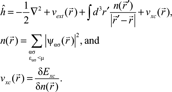
In the Schrödinger equation, the motion of each electron is coupled to the motion of every other electron through Coulomb repulsion among the electrons. As a result, the computational time increases very rapidly with the number of electrons in the system, so this method is impractical for large molecules or nanostructures or many other real materials. A computationally efficient alternative is the Kohn–Sham DFT, developed in 1965,^{Reference Kohn and Sham1} for which Walter Kohn received the Nobel Prize in Chemistry in 1998.^{Reference Kohn8} The main idea of the theory is that we can, in principle, find the exact ground-state energy E and the exact ground-state electron density $n\left( {\vec r} \right)$ by solving an effective one-electron Schrödinger equation:

(1)$$\hat h{\rm{\psi }}_{{\rm{\alpha \sigma }}} = {\rm{\varepsilon }}_{{\rm{\alpha \sigma }}} {\rm{\psi }}_{{\rm{\alpha \sigma }}} ,$$

(2)$$\eqalign{ & \hat h = - {1 \over 2}\nabla ^2 + v_{ext} (\vec r) + \int {d^3 } r'{{n(\vec r')} \over {\left| {\vec r' - \vec r} \right|}} + v_{xc} (\vec r), \cr & n(\vec r) = \sum\limits_{\scriptstyle {\rm{\alpha \sigma }} \hfill \atop \scriptstyle {\rm{\varepsilon }}_{{\rm{\alpha \sigma }}} {\rm{ < \mu }} \hfill} {\left| {{\rm{\psi }}_{{\rm{\alpha \sigma }}} (\mathord{\buildrel{\lower3pt\hbox{$\scriptscriptstyle\rightharpoonup$}}\over r} )} \right|} ^2 ,\,{\rm{and}} \cr & v_{xc} (\vec r) = {{{\rm{\delta }}E_{xc} } \over {{\rm{\delta }}n(\vec r)}}. \cr} $$

Here $\vec r$ and $\vec r'$ are different positions in space.

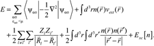
It is much easier to deal with a wave function for one electron (an orbital) than to deal with a correlated wave function for N electrons when N is large. Equation 1 is a one-electron Schrödinger equation with a one-electron Hamiltonian (Equation 2), which is actually an effective Hamiltonian because it includes (in order of presentation) the kinetic energy of that electron, the interaction of that electron with the external potential from the nuclei, the Coulomb repulsion of the electron density acting on that electron, and the exchange-correlation potential, which is only a function of position but in practice has to be approximated. Similarly, the total energy consists of a similar series of terms:

(3)$$E = \sum\limits_{\scriptstyle {\rm{\alpha \sigma }} \hfill \atop \scriptstyle {\rm{\varepsilon }}_{{\rm{\alpha \sigma }}} {\rm{ < \mu }} \hfill} {\left\langle {{\rm{\psi }}_{{\rm{\alpha \sigma }}} \left| { - {1 \over 2}\nabla ^2 } \right|{\rm{\psi }}_{{\rm{\alpha \sigma }}} } \right\rangle } + \int {d^3 r} n(\vec r)v_{ext} (\vec r) + {1 \over 2}\sum\limits_{l \ne l'} {\sum\limits_{l'} {{{Z_l Z_{l'} } \over {\left| {\mathord{\buildrel{\lower3pt\hbox{$\scriptscriptstyle\rightharpoonup$}}\over R} _l - \mathord{\buildrel{\lower3pt\hbox{$\scriptscriptstyle\rightharpoonup$}}\over R} _{l`} } \right|}}} } + {1 \over 2}\int {d^3 r} \int {d^3 r'{{n(\vec r)n(\vec r')} \over {\left| {\vec r' - \vec r} \right|}}} + E_{xc} \left[ n \right].$$

Equation 3 includes (in order of presentation) the kinetic energy for all of the electrons (obtained from the expectation value of the kinetic energy operator using each occupied orbital), the interaction of the electron density with the external potential, the Coulomb repulsion among the nuclei, and Coulomb repulsion among the electrons. The last term is the exchange-correlation energy E _xc as a function of the electron density $n(\vec r)$; E _xc[n] must also be approximated in this theory. The two quantities that must be approximated are related; we obtain the exchange-correlation potential by taking the functional derivative of the exchange-correlation energy with respect to the density. So, in practice, we only need to approximate E _xc. If we knew the exact E _xc as a functional of the density, we could predict the exact ground-state energy and the exact ground-state density by solving these Kohn-Sham equations self-consistently. In practice, the exact E _xc cannot be computed, and we need to make approximations. The way we make these approximations is the main subject of this talk.

A functional is a rule that assigns a number to a function. In this case, it is a rule that assigns an energy, a scalar number, to each electron density $n\left( {\vec r} \right)$. The exchange-correlation energy is a negative energy that represents the lowering of the energy of the system due to the fact that the electrons avoid each other as they move through the density. The electrons are like a swarm of bees. There is an average density of bees, which is a function of position, and the bees move around within this swarm, but they do not move completely randomly because they sense each other, and they avoid each other. Electrons do the same. Because of the Pauli principle and Coulomb repulsion, electrons avoid each other. This lowers their electrostatic energy, and this energy reduction is the exchange-correlation energy (apart from a small positive piece that represents the kinetic energy of correlation). It is a relatively small fraction of the total energy, but it is very important for all aspects of materials science, because the exchange-correlation energy is what I refer to as “nature’s glue.”^{Reference Kurth and Perdew9} It binds the atoms together into molecules and solids. Without this energy, the atoms would either not be bound together or they would be too loosely bound with weak binding energies and long bond lengths. Without E _xc, we would have a completely unrealistic description of materials.

Local density approximation

How do we approximate this exchange-correlation energy functional? The earliest approximation was the local density approximation (LDA) of Kohn and Sham.^{Reference Kohn and Sham1} This is a non-empirical approximation, in the sense that it has no parameter fitted to experimental data. Instead, it uses information about the uniform electron gas, obtained from accurate quantum mechanical calculations, for example from quantum Monte Carlo computations, from which we obtain the exchange-correlation energy per electron of an electron gas of uniform density n. The density is assumed to be uniform over all space. This is a solvable problem. We then treat a nonuniform system—a real atom or molecule or solid—as if it locally consisted of infinitesimal volume elements, each of which is a locally uniform electron gas. This assumption leads to Equation 4:

(4)$$E_{_{xc} }^{LDA} [n] = \int {d^3 r} n(\vec r){\rm{\varepsilon }}_{xc}^{unif} (n(\vec r)),$$

where ${\rm{\varepsilon }}_{xc}^{unif} (n)$ is the exchange-correlation energy per particle of an electron gas of uniform density n.^{Reference Perdew and Wang10,Reference Vosko, Wilk and Nusair11}

Kohn and Sham proposed this approximation in 1965. It started to become popular in the early 1970s, when solid-state physicists began to realize that they could obtain accurate results for lattice constants, phonon frequencies, and other properties they wanted to calculate using this approximation. The approximation is exact for a uniform density, and it is correct and accurate for a density that varies slowly over space, but, in fact, it also works reasonably well for atoms, molecules, and surfaces. This was surprising at the time, but the reason was understood in the 1970s:^{Reference Langreth and Perdew12,Reference Gunnarsson and Lundqvist13} The LDA satisfies certain exact constraints on the exchange-correlation energy as a functional of the density. In other words, it includes certain features of the exchange-correlation energy that remain true even when the density is far from uniform. That explanation was the basis for a ladder^{Reference Perdew, Schmidt, Van Doren, Van Alsenoy and Geerlings14} of approximations of increasing sophistication to this exchange-correlation energy (see Figure 1). Today, most chemists and many materials scientists use a higher rung of the ladder than the LDA.

Figure 1.

Jacob’s ladder of density functional approximations. The rungs are labeled on the left, and their added ingredients are shown on the right.

Jacob’s ladder of density functional approximations

The strategy behind the construction of the ladder is to try to include additional exact constraints into approximations beyond the LDA, in the hope that those additional exact constraints will make the functional even more accurate. I call this hierarchy “Jacob’s ladder of density functional approximations.”^{Reference Perdew, Schmidt, Van Doren, Van Alsenoy and Geerlings14} In the Bible, the patriarch Jacob dreamed of a ladder reaching from earth up to heaven, with the angels ascending and descending. In the Jacob’s ladder of density functional approximations, earth is the Hartree approximation (E _xc = 0), and heaven is the realm of high accuracy. The angels are the users, who can choose the rung that best fits their needs and computational resources. The basic idea is that the exchange-correlation energy is written as an integral over the three-dimensional space of some function ${\rm{\varepsilon }}_{xc}^{approx}$ of the local density $n\left( {\vec r} \right)$ at each point $\vec r$, the gradient or derivative of the local density $\nabla n\left( {\vec r} \right)$ at each point $\vec r$, and possibly some other ingredients, such as the orbital kinetic energy density $\tau (\vec r)$,

(5)$$E_{xc}^{approx} [n] = \int {d^3 rn(\vec r){\rm{\varepsilon }}_{xc}^{approx} \left( {n(\vec r),\nabla n(\vec r),{\rm{\tau }}(\vec r),...} \right)} ,$$

where ${\rm{\tau }}(\vec r) = {1 \over 2}\sum\limits_{\scriptstyle {\rm{\alpha \sigma }} \hfill \atop \scriptstyle {\rm{\varepsilon }}_{{\rm{\alpha \sigma }}} {\rm{ < \mu }} \hfill} {\left| {\nabla {\rm{\psi }}_{{\rm{\alpha \sigma }}} (\vec r)} \right|} ^2 $ is the positive kinetic energy density.

The lowest rung of the ladder is the LDA,^{Reference Kohn and Sham1,Reference von Barth and Hedin15} which employs only the local density. The second rung of the ladder is the generalized-gradient approximation (GGA),^{Reference Langreth and Perdew16–Reference Perdew, Burke and Ernzerhof19} which adds a second ingredient, the gradient of the density. The third rung is the meta-GGA,^{Reference Becke20–Reference Sun, Haunschild, Xiao, Bulik, Scuseria and Perdew25} which adds a third ingredient, the orbital kinetic energy density. These first three rungs are semi-local functionals that are computationally very efficient. The fourth and fifth rungs are non-local functionals, which are computationally more expensive because they require at least a double integration over three-dimensional space but are potentially more accurate. On the fourth rung, we have hybrid functionals^{Reference Becke26–Reference Adamo and Barone29} that use some exact exchange information, such as the exact exchange energy density or the exact exchange energy itself. On the fifth rung, we have the random-phase-approximation-like functionals^{Reference Langreth and Perdew16,Reference Furche30,Reference Harl, Schimka and Kresse31} that use the unoccupied Kohn–Sham orbitals, and on that rung DFT starts to resemble traditional many-body theory.

The orbital kinetic energy density is a positive quantity obtained by summing the squares of the gradients of the occupied orbitals. We can obtain the orbitals from a Kohn–Sham calculation, and then we can easily compute ${\rm{\tau }}(\vec r)$. In the ladder strategy, when we add an ingredient, we can satisfy additional exact constraints, and we can achieve greater accuracy, but for some increase in computational cost.

Some of the exact constraints will now be described. We know a great deal about the exchange-correlation energy, thanks to work by David Langreth, Olle Gunnarson, Bengt Lundqvist, Mel Levy, and others. We also know several exact expressions for E _xc. They are not computable in practice, but they are formally exact, for example:^{Reference Langreth and Perdew12,Reference Gunnarsson and Lundqvist13}

(6)$$E_{xc} = {1 \over 2}\int {d^3 r} n(\vec r)\int {d^3 } r'{{n_{xc} (\mathord{\buildrel{\lower3pt\hbox{$\scriptscriptstyle\rightharpoonup$}}\over r} ,\mathord{\buildrel{\lower3pt\hbox{$\scriptscriptstyle\rightharpoonup$}}\over r} ')} \over {\left| {\mathord{\buildrel{\lower3pt\hbox{$\scriptscriptstyle\rightharpoonup$}}\over r} - \mathord{\buildrel{\lower3pt\hbox{$\scriptscriptstyle\rightharpoonup$}}\over r} '} \right|}} = E_x + E_c ,$$

where $n_{xc} (\mathord{\buildrel{\lower3pt\hbox{$\scriptscriptstyle\rightharpoonup$}}\over r} ,\mathord{\buildrel{\lower3pt\hbox{$\scriptscriptstyle\rightharpoonup$}}\over r} ') = n_x (\vec r,\vec r') + n_c (\vec r,\vec r')$ is the density at $\mathord{\buildrel{\lower3pt\hbox{$\scriptscriptstyle\rightharpoonup$}}\over r} '$ of the (coupling-constant averaged) exchange-correlation hole (xc hole) around an electron at $\mathord{\buildrel{\lower3pt\hbox{$\scriptscriptstyle\rightharpoonup$}}\over r} $, with

$$n_x (\mathord{\buildrel{\lower3pt\hbox{$\scriptscriptstyle\rightharpoonup$}}\over r} ,\mathord{\buildrel{\lower3pt\hbox{$\scriptscriptstyle\rightharpoonup$}}\over r} ') \le 0,\,\int {d^3 } r'n_x (\mathord{\buildrel{\lower3pt\hbox{$\scriptscriptstyle\rightharpoonup$}}\over r} ,\mathord{\buildrel{\lower3pt\hbox{$\scriptscriptstyle\rightharpoonup$}}\over r} ') = - 1,\,{\rm{and}}\,\int {d^3 } r'n_c (\mathord{\buildrel{\lower3pt\hbox{$\scriptscriptstyle\rightharpoonup$}}\over r} ,\mathord{\buildrel{\lower3pt\hbox{$\scriptscriptstyle\rightharpoonup$}}\over r} ') = 0.$$

Equation 6 tells us that the exchange-correlation energy is the electrostatic interaction between the electron density at point $\mathord{\buildrel{\lower3pt\hbox{$\scriptscriptstyle\rightharpoonup$}}\over r} $ and the density at point $\mathord{\buildrel{\lower3pt\hbox{$\scriptscriptstyle\rightharpoonup$}}\over r} '$ of the exchange-correlation (xc) hole that surrounds an electron at $\mathord{\buildrel{\lower3pt\hbox{$\scriptscriptstyle\rightharpoonup$}}\over r} $. This can be divided into an exchange part and a correlation part in a very simple way, and the exact expressions also provide us with certain properties of the hole—exact constraints that can be used to model the functional. For instance, the exchange hole density is non-positive everywhere. The integral of the exchange hole density is –1, and the integral of the correlation hole density is zero. So the idea of the exchange-correlation hole is similar to that of the personal space around a bee in a swarm. There is a region of space around each bee, which the other bees tend to avoid, and this creates a hole in the density. The same thing is true for electrons—each electron is surrounded by a hole in the density, from which we can obtain the exchange-correlation energy.

These constraints help to explain why the LDA works better than expected. The exchange-correlation hole of the LDA is negative, with an integral of –1, and its correlation hole density integrates to zero. These constraints are satisfied automatically by LDA, not only for uniform density but for any density.^{Reference Langreth and Perdew12,Reference Gunnarsson and Lundqvist13} There are other exact constraints that have been discovered over the years, applicable not to the hole but more directly to the energy. If the density varies slowly over space, there is a density gradient expansion for the exchange-correlation energy.^{Reference Ma and Brueckner32–Reference Svendsen and von Barth34} If the density is scaled uniformly or non-uniformly, there are scaling relations, equalities, and inequalities for the exchange and correlation energies.^{Reference Levy and Perdew35,Reference Levy36} There is a Lieb–Oxford lower bound on the exchange-correlation energy,^{Reference Lieb and Oxford37} and there are many other known exact constraints. The higher-level approximations on the higher rungs of the ladder attempt to keep the constraints satisfied by the lower-level rungs, and then add additional constraints in the hope that they will lead to a more accurate functional, and typically they do.

The Hamiltonian in Equation 1 has no magnetic field, which means there is nothing that couples to the z-components of the spin or to the current density, and as a result, we only require, in principle, the exchange-correlation energy as a functional of the total density. If we have external fields that couple to the z-component of the electron spin, then we need to include the up- and down-spin electron densities; that is spin-DFT.^{Reference von Barth and Hedin15} In practice, even if there is no such field coupling to the spin, we use spin-density functionals to achieve higher accuracy at a given level of approximation. It is not difficult to see the reason for this. More information is inputted to a spin-density functional than to a density functional, so the spin-density functional approximations typically work better and provide more useful outputs.

Spin-density functionals are especially useful for open-shell systems, such as typical atoms.^{Reference Gunnarsson, Lundqvist and Wilkins38} We can also use spin-DFT to predict spontaneous magnetization, such as the ferromagnetism of iron. Approximations sometimes predict a spurious spin-symmetry breaking,^{Reference Gunnarsson and Lundqvist13} which leads to a spurious spin density but to a significant improvement in the exchange-correlation energy and in the total energy. This tends to happen in strongly correlated systems. An example of this is stretched H₂. We take the H₂ molecule, stretch out the bond length toward infinity, and try to describe that system through spin-DFT. At some large bond length, the spin symmetry will break in a semi-local approximation, which will no longer yield a singlet ground state but instead will yield a broken-symmetry state with spin up on one nucleus and spin down on the other. This is actually a better description, because it is similar to having separated atoms, so this spin-symmetry breaking can be good for describing the energy at the semi-local level. To simplify the notation, $n_ \uparrow$ and $n_ \downarrow$ will not be shown, but in practice, all the functionals considered here are spin-density functionals.

Approximation desiderata

What are we looking for when we make an approximation to the exchange-correlation energy? There are three properties that are useful in an approximate functional:

1. (1) The approximation should be non-empirical. It should be constructed from exact constraints or from a derivation and not from fitting to data sets. The reason is that non-empirical functionals tend to be more universally useful, because the constraints themselves are universal. Non-empirical functionals tend to work for wider classes of systems than functionals fitted to data sets, and they also provide a better test of our understanding of the physics of the exchange-correlation energy. So if a non-empirical functional works, it is probably because we understood something. If an empirical functional works, it works in part because it was fitted. The first three rungs of our ladder, which define the semi-local functionals—local density approximation, GGA, and meta-generalized-gradient approximation—are semi-local; they are not fully non-local, and we have non-empirical constructions for functionals on all of those rungs. On the fourth rung, we have the hybrid functionals, which can be very accurate, but typically they have at least one empirical parameter, and some of them have as many as 40 empirical parameters. The fifth rung includes the random phase approximation (RPA), where we once again have a non-empirical approximation, but we still need to make corrections to the RPA because it is not exact, and, to date, the best corrections are empirical. So the first three rungs are almost completed and non-empirical, and the fourth and fifth rungs still contain some empiricism.

2. (2) We require this functional to be computationally efficient. When we perform a calculation for a material, we would like to have a result in a week or even in a few days or a few hours. The semi-local functionals are all computationally very efficient, because they evaluate the exchange-correlation energy as a single integral over three-dimensional space, which is computationally simple. The hybrid functionals, which require some exact exchange component, such as the exact exchange energy density,^{Reference Jaramillo, Scuseria and Ernzerhof39,Reference Perdew, Staroverov, Tao and Scuseria40} can be slower by a factor of 10 or 100, depending on the system and on the numerical program used. The random phase approximation can be 100 times slower than the semi-local functionals. Semi-local functionals require approximately the same computer time. GGA is possibly twice as slow as LDA, while the meta-GGA might require another 30% of the computer time compared to the GGA. That is quite acceptable, because it is not a factor of 10 or 100.

3. (3) Finally, we require our approximations to be accurate. The approximations need not be exact, but they must provide useful information.

Local density approximation

Let us consider some of these functionals, starting with the LDA^{Reference Kohn and Sham1} or the local spin-density approximation (LSDA):^{Reference von Barth and Hedin15}

• • It satisfies the exchange-correlation hole sum rules.^{Reference Langreth and Perdew12,Reference Gunnarsson and Lundqvist13}

• • It is exact for uniform densities.^{Reference Perdew and Wang10,Reference Vosko, Wilk and Nusair11}

• • It satisfies some of the scaling relations.^{Reference Levy and Perdew35,Reference Levy36}

• • It satisfies the general Lieb–Oxford lower bound.^{Reference Lieb and Oxford37}

• • It is accurate for the linear response of a uniform density.^{Reference Moroni, Ceperley and Senatore41}

In practice, the LDA is useful for some simple solids. It predicts lattice constants that are typically 1% or 2% too short, and it predicts total surface energies that are rather realistic. However, if we examine the atomization energy—the energy to break a material or a molecule up into atoms—we find that the LDA yields very serious errors, strongly over-binding atoms into molecules and onto surfaces. So the LDA is not used much in chemistry, but if we are not interested in breaking off atoms, then LDA often works very well.

Generalized gradient approximation

The second rung of the ladder is the GGA,^{Reference Langreth and Perdew16–Reference Perdew, Burke and Ernzerhof19} which can be constructed to satisfy different sets of exact constraints. There is some incompatibility associated with the limited form of the GGA—we can satisfy some subset of possible constraints, but we cannot satisfy all of them with the same GGA, so we need to select the constraints. One of the standard GGAs is the Perdew–Burke–Ernzerhof (PBE) approximation.^{Reference Perdew, Burke and Ernzerhof19} PBE recovers the second-order gradient expansion for correlation for a slowly varying density, while preserving the accurate LSDA linear response of a uniform density. It adds a scaling relation for correlation that LSDA does not satisfy. With regard to accuracy, the PBE GGA substantially reduces and improves the overbinding of atoms into molecules and solids. It still overbinds in most cases but much less than LSDA. PBE overcorrects the lattice constants. Calculated lattice constants are too short in LDA, and they are a little too long in GGA. Also, if we examine the surface energy, we find that PBE improves the separate exchange surface energy and correlation surface energy, but the sum of the two is actually less accurate than in LDA. Despite its shortcomings, PBE is still a useful functional.

There is a variant of GGA, “PBEsol”^{Reference Perdew, Ruzsinszky, Csonka, Constantin, Zhou, Vydrov, Scuseria and Burke42} or “PBE for solids,” which, unlike PBE, recovers the second-order gradient expansion for the exchange energy over a wide range of slowly varying densities. This is an alternative set of constraints to satisfy; instead of recovering the linear response of the uniform gas, this approximation satisfies the gradient expansion of the exchange energy. PBEsol is in some sense between LDA and PBE. It works very well for simple solids (as do other GGAs for solids)^{Reference Armiento and Mattsson43,Reference Wu and Cohen44} and gives accurate lattice constants and accurate surface energies. It can be useful for many solid-state problems, but it is not useful for chemistry problems, because the atomization energies are still too large, somewhere between the strongly overbound LDA atomization energies and the moderately overbound PBE atomization energies. In order to have a really accurate description of typical atoms, molecules, and solids near their equilibrium geometries—an important desideratum—we need to climb to the third rung, the meta-GGA level.

Meta-GGA approximation

Meta-GGAs^{Reference Becke20–Reference Sun, Haunschild, Xiao, Bulik, Scuseria and Perdew25} have another ingredient—the orbital kinetic energy density—and we can use that ingredient to satisfy some additional exact constraints. For instance, we can recover the gradient expansion of the exchange energy—not just to the second order as in PBEsol but even to the fourth order^{Reference Svendsen and von Barth34} in the gradients. At the same time, we can preserve an accurate linear response of the uniform density, which means that the GGA need to select constraints is avoided. The meta-GGAs can also cancel out the correlation energy for any one-electron density, which is desirable because a one-electron system has no correlation. We can also calculate the exchange energy exactly, not for all densities but for some particular density, such as the density of a one-electron atom. By using this extra ingredient—the orbital kinetic energy density—meta-GGA can recognize regions of space in which one orbital shape dominates the electron density. For instance, in the hydrogen and helium atoms, there is only one orbital shape per atom. In a typical covalent chemical bond, there is one dominant orbital shape—the shape of the bonding orbital, and these regions can be treated differently from regions of slowly varying density, even when the density gradient reduces to zero. This means that the meta-GGA is able to recognize the difference between a slowly varying density and a one- or two-electron ground-state density, and this capability has proved to be very useful in correctly describing both solid-state physics and chemistry.

One of the meta-GGAs that we favor is revTPSS^{Reference Perdew, Ruzsinszky, Csonka, Constantin and Sun23} (a revised Tao–Perdew–Staroverov–Scuseria^{Reference Tao, Perdew, Staroverov and Scuseria22} meta-GGA). In comparison with GGAs, it gives accurate lattice constants for solids simultaneously with accurate surface energies and accurate binding energies for atoms, as well as the binding energies of molecules to surfaces. It performs a number of calculations needed in materials science very well.^{Reference Wu and Cohen44–Reference Hao, Sun, Csonka, Philipsen and Perdew46} My group recently developed a “meta-GGA made simple,”^{Reference Sun, Xiao and Ruzsinszky24,Reference Sun, Haunschild, Xiao, Bulik, Scuseria and Perdew25} which can even describe intermediate-range van der Waals interactions that are important for the chemistry and physics of soft matter but are less-reliably described in GGAs and in the revTPSS meta-GGA. These semilocal functionals—LDA, GGA, and meta-GGA—will never get the long-range part of the van der Waals interaction right, which requires a nonlocal functional like the RPA. However, they can, in fact, describe the short- and intermediate-range part of the van der Waals interaction, which can be important for binding one atom to another in soft matter. For instance, in graphite, one layer of carbon atoms is bound to the next layer of carbon atoms, not by a covalent bond or a metallic bond, but rather by a van der Waals bond, and much of that van der Waals bond is described by this “meta-GGA made simple.” At the same time, it performs like revTPSS for calculating the other properties previously mentioned.^{Reference Sun, Haunschild, Xiao, Bulik, Scuseria and Perdew25}

If we have a system that is near mechanical equilibrium, where the bond lengths and the lattice constants are close to their equilibrium values, then a meta-GGA can come very close to satisfying our three desiderata: (1) It is typically non-empirical—there is no need to fit to experimental data sets. (2) It is computationally efficient—not much slower than the LDA. (3) And it has useful accuracy for atoms, molecules, solids, and surfaces for a wide range of systems we might be interested in, provided the bonds are not stretched too much. Meta-GGAs are now available in many standard electronic-structure codes for molecules and solids, including VASP and GAUSSIAN.

We would like to improve the meta-GGA, and we think this is possible because it is a very flexible form. Even for a spin-unpolarized system, it has three arguments. There are rich possibilities for building a better meta-GGA, and we would like to build one that will satisfy all the exact constraints that can be satisfied by a meta-GGA, including one that no one has ever tried to satisfy before, the tight Lieb–Oxford lower bound on the exchange energy of any one-electron density.^{Reference Lieb and Oxford37} The exchange energy of any one-electron density is very tightly bounded by its Lieb–Oxford lower bound, which means that the functional is almost determined by the lower bound for one-electron densities, and we would like to make use of this. We think that such a meta-GGA could be useful in its own right, but it could also be the basis for the construction of a more accurate fully non-local functional, for instance, via the Perdew–Zunger self-interaction correction,^{Reference Perdew and Zunger47} which removes (on an orbital-by-orbital basis) the self-interaction error that all semi-local functionals have in their exchange part. A meta-GGA can be a component of a hybrid functional, where typically we mix in some exact exchange, and it can also be used in RPA to help make the short-range correction to that approximation.

Stretched bonds

What happens when we deviate from equilibrium bond lengths? If we have stretched bonds, the functionals typically need to be non-local.^{Reference Perdew, Staroverov, Tao and Scuseria40} When bonds are stretched, the exact exchange-correlation hole around an electron can spread out over two or more atomic centers. A classic example of this is stretched H₂⁺. This is a molecule with two protons and one electron. The distance between the protons is greatly elongated, so that when the electron is sitting on one of the nuclear centers, half of its exchange hole is on that center and half is on the far-distant center. This situation cannot be described by a semi-local functional. It requires real non-locality, and without that non-locality, we have an incorrect description. The semi-local approximations localize the exchange-correlation hole around its electron, which means in this case the calculated exchange-correlation energy is too negative for stretched H₂⁺. This is a typical self-interaction error, and it can only be corrected by a non-local approximation. These stretched bonds arise in binding energy curves. If we take a binding energy curve for a molecule and stretch out a bond length, and if an electron is shared between the two ends of the bond, there will eventually be a problem—a failure of the semi-local functionals.

Non-local stretched bonds also arise in the transition states of chemical reactions. When two molecules come together, they form a transition state, a complex or super-molecule. In this super-molecule, the bonds are typically weak and long. They are effectively stretched bonds, in which there is a significant non-locality. In order to describe the barrier height to a chemical reaction—the energy of the transition state, which is typically higher than the energy of the reactants or of the products—we must include real non-locality in our functional.

If we examine systems that have atomic-like d and f electrons, then even at equilibrium the d and f bonds can be stretched. Of course, the total bond is in equilibrium, but if we think of the bond as being made up of an s part and a d part, then the d part may actually be stretched, and so we also have such effects potentially occurring in these systems, which are often called “strongly correlated systems.” The transition-metal oxides such as NiO and VO₂ are well-known examples. With the right amount of non-locality, we might also obtain a better description of strongly correlated materials, and this requires the two highest rungs of the ladder, either the hybrid functionals or the RPA-like functionals, to describe these stretched-bond, strongly correlated situations.

Hybrid functionals

Hybrid functionals^{Reference Becke26–Reference Adamo and Barone29} include an exact exchange component. One of the simplest of these is the PBE0 hybrid,^{Reference Perdew, Ernzerhof and Burke27–Reference Adamo and Barone29} which mixes a fraction of exact exchange with a complementary fraction of PBE-GGA exchange and full PBE correlation. A typical fraction is 25% exact exchange. We can think of that 25% as a semi-empirical parameter, because the non-empirical argument for it^{Reference Perdew, Ernzerhof and Burke27} is not precise. This functional is usually much more accurate than PBE for the atomization energies of molecules and lattice constants of solids. It also improves the calculation of surface energies and energy barriers, compared to PBE. It gives improved but still inaccurate dissociation limits, but this is at least an improvement on semi-local functionals. We can also obtain a better prediction of energy gaps in materials,^{Reference Brothers, Izmaylov, Normand and Scuseria48} because the potential in the hybrid functional is not a Kohn–Sham local potential but a mixture of a Hartree–Fock non-local potential with a Kohn–Sham local potential. (Hartree–Fock theory gives the energetically best non-interacting wave function to approximate the true correlated wave function.) The non-locality in the potential can mimic that of the self-energy and provide a reasonable description of bandgaps that would not be accurate even from the orbital energies of the exact Kohn–Sham density functional.

One criticism is that all successful hybrid functionals require at least one empirical parameter, and some have as many as 40. This means that we are missing some understanding of how to construct them. We are trying to develop non-empirical hybrids, for instance based on models for the exchange-correlation hole that use the exact exchange hole as an input.

Random phase approximation

The fifth-rung functionals are the RPA-like functionals.^{Reference Langreth and Perdew16,Reference Furche30,Reference Harl, Schimka and Kresse31} RPA in a density functional context was proposed in the 1970s. It is a many-body approximation that includes unoccupied Kohn–Sham orbitals, unlike the first four rungs, which use only the occupied orbitals. RPA is nearly exact for the long-range part of the exchange-correlation hole, but the short-range part is in error. The total error from RPA is actually very large, –0.5 eV per electron in a typical system. That is a huge error, but almost all of that error cancels out from the energy differences we are interested in, if we make a change in the system that leaves the number of electrons unchanged. RPA can actually be useful for materials science, even without a correction, because of this remarkable cancellation of errors. For molecules, the error cancellation is somewhat imperfect,^{Reference Furche30} so by itself the RPA is not very useful. However, Georg Kresse applied the RPA to solids in the past few years (e.g., Reference 30), and he found a much more nearly perfect error cancellation—similar to the error cancellation we had expected^{Reference Yan, Perdew and Kurth49} to find in the 1990s. Kresse and others have found that RPA can yield very accurate lattice constants, surface energies, cohesive energies, and solid-state reaction energies. In our group, we have also found that RPA can yield accurate structures and accurate transition pressures^{Reference Xiao, Sun, Ruzsinszky, Feng and Perdew50} for structural phase transitions in solids. RPA also provides a good description of the long-range van der Waals interaction, which is missing from the first four rungs of the ladder. The RPA and the hybrid functionals—the fully non-local functionals—are available in VASP and other codes. We would like to construct a non-empirical non-local correction to RPA, which is required more for molecules than for solids.

Summary

Kohn–Sham density functional theory is currently the most widely used method for electronic structure calculation in materials science, condensed matter physics, and quantum chemistry, used not only by theorists but even by experimentalists. It is neither the only method nor the most accurate one, but it is often a very efficient and useful method. This method has a rigorous foundation for ground-state energies, ground-state electron densities, and geometric structures (i.e., equilibrium positions of the nuclei). It also has a hierarchy of approximations—the “Jacob’s ladder”—of increasing sophistication for the exchange-correlation energy as a functional of the density. The ladder is still not complete. From my point of view, the first two rungs are complete, but we can still improve the third, fourth, and fifth rungs, and hopefully we can therefore make the functionals more accurate, more non-empirical, and more useful.