Over the last decade, there has been renewed interest in determining whether inequality affects the development of commercial banks and credit. Stanley Engerman, Elisa Mariscal, and Kenneth Sokoloff (Reference Engerman, Mariscal and Sokoloff2002) and Raghuram Rajan (Reference Rajan2009) argue that the existence of a large gap between “haves” and “have nots” may have been sufficient to establish inefficient institutions. According to Rajan (Reference Rajan2009, p. 1): “When citizens in a poor constrained society are very unequally endowed, they are likely to find it hard to agree on reforms, even though the status quo hurts them collectively.” Engerman and Sokoloff (Reference Engerman and Sokoloff2002), Douglas North, John Wallis, and Barry Weingast (Reference North, Wallis and Weingast2009), and Daron Acemoglu and James Robinson (Reference Acemoglu and Robinson2012) argue that elites in most societies use their endowments to shape institutions in order to maintain their preferred access to economic opportunities. On the other hand, they also show that some societies have successfully made the transition from governments dominated by elites to open access societies where large numbers of people are free to compete and improve their economic welfare. While the United States successfully made this transition early in its development, Jonathan Weiner (Reference Weiner1975) and Oded Galor, Omer Moav, and Dietrich Vollrath (Reference Galor, Moav and Vollrath2009) raise questions about the openness of the southern economy even after the Civil War.
Rajan and Rodney Ramcharan (Reference Rajan and Ramcharan2011) performed a test of the hypothesis that settings with more inequality lead to restricted access to credit in lesser developed economies. Specifically, they examined the relationship between inequality in the size of farm operations and the extent of banking activity in 1920s America. They argued that elites were providing informal credit to small farmers and tenants and saw commercial banks as potential rivals in the provision of that type of credit; therefore, the elites worked to prevent commercial banks from developing in their areas. Their results show that greater inequality in the size of farm operations was associated with less bank activity per capita in the 1920s.
In this article we create a new dataset that covers all banks in the United States in the census years between 1870 and 1900 to test the relationship between inequality and banks during the late nineteenth century when the provision of informal credit by local elites in the agricultural sector was at its height. The combination of the Civil War, the National Banking Acts, and a tax on state bank notes led to the general absence of commercial banks in agricultural counties throughout the nation in 1870. The situation in the South was compounded further by the end of slavery, which led to substantial changes in the economic and institutional relationships between elites and their work force.
Our findings suggest that the relationship between inequality and bank activity in rural economies changed substantially between 1870 and 1900–1920. In the early phases when the banking sector was starting over from scratch after the National Banking Acts and the Civil War, elites appear to have taken action to start or attract banks to build up access to credit in their counties. After 1900, when nearly all counties had at least one bank and many had multiple banks, it looks more like a situation where the elites who were trying to stop bank entry were the bank owners themselves rather than the plantation owners and merchants who were making consumption loans to croppers and tenants. After all, many of the plantation owners and merchants were themselves borrowing from the banks and likely would have welcomed more competition among bankers when seeking credit.Footnote 1
REBUILDING THE COMMERCIAL BANKING SYSTEM IN THE POST-BELLUM PERIOD
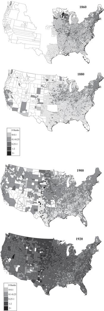
Access to existing state banks (including state banks, trust companies, and savings banks) was virtually eliminated in the nation's agricultural areas during the 1860s. Nearly all southern banks closed during the Civil War, whereas many rural Midwest banks closed after a prohibitive tax on state bank notes was passed in 1865 (Jaremski Reference Jaremski2013). Following the Civil War, national banks emerged and state banks rebounded. The number of incorporated banks grew from around 2,000 banks to more than 10,000 by 1900, but Figure 1 shows that growth was more concentrated in the Northeast and Midwest, than in southern agricultural areas. Even as late as 1900, 30 percent of southern counties did not have a bank, compared to 15 percent of non-southern counties.
TOTAL NUMBER OF BANKS PER THOUSAND PEOPLE BY COUNTY (1860–1920)

Largely due to a lack of a formal charter or specific regulation, private bankers fared somewhat better during the Civil War. Their number nearly doubled between 1860 and 1870. They typically had very small capital levels. In cities they were often adjuncts to brokerage businesses, while many operated in small communities and agricultural areas where there was not sufficient capital or people to create an incorporated bank (Barnett Reference Barnett1911, p. 206). That said, while private brokerage banks expanded in financial centers such as Chicago and New York City, the growth of private bankers across southern agricultural areas was slow over the late 1800s, especially as capital requirements of state and national banks were lowered.Footnote 2
There are several potential reasons why banks did not return quickly to agricultural areas after the Civil War. National banks were largely prohibited from providing loans on real estate, and banks tended to make short-term loans to finance operating expenses rather than long-term mortgages, which led to short-term, self-liquidating loans. Therefore, unlike the 1920s decade studied by Rajan and Ramcharan, the majority of bank loans before 1900 provided operational and seasonal liquidity rather than long-term mortgage debt. Kenneth Snowden (Reference Snowden, Lamoreaux and Raff1995, Table 7.1, p. 220) reports that only 30 percent of all U.S. mortgage debt around 1890 was provided by financial intermediaries, and the share was lowest in the agricultural South (12 percent) and Midwest (28 percent). Moreover, mortgages in these agricultural regions were often from building and loan associations, life insurance companies, and large mortgage companies rather than standard banks.
Lewis Haney (Reference Haney1914) and Richard Keehn and Gene Smiley (Reference Keehn and Smiley1977) argue that some national banks circumvented the restrictions, but the evidence indicates that mortgages at national banks were relatively uncommon. Indeed, state banks lent a much larger proportion and value of their funds on real estate. According to the Board of Governors of the Federal Reserve System (1959), more than 40 percent of all loans by state banks, trust companies, and savings banks in 1896 were on real estate compared to 9 percent by national banks. While the Board of Governors only lists private bankers for a few states, the data suggest that they too provided few mortgages.
National bank capital requirements and a prohibitive tax on state bank notes are a frequently cited reason for the lack of incorporated banks in rural communities (Sylla Reference Sylla1969). The National Banking Act of 1864 required national banks in a city with more than 50,000 people to have $200,000 in capital, those with 6,000 to 49,999 people to have $100,000, and those in smaller cities to have $50,000.Footnote 3 The intent was to prevent the emergence of risky and undercapitalized banks, but the result was the elimination of national banks in many rural areas. State banks generally had lower capital requirements, but their inability to issue bank notes slowed their growth until deposit accounts became more popular.Footnote 4 As a result private bankers often were able to operate in rural areas without much competition from incorporated banks.
Even in the short run, agricultural lending was inherently risky. Bad local weather or good foreign weather would dramatically affect farmers' ability to repay their loans. Barry Eichengreen (Reference Eichengreen1984, Reference Eichengreen1987) and Snowden (Reference Snowden1987) argue that greater risk and higher transactions costs contributed to higher interest rates on mortgages in the West and South than in the East in the early 1890s.Footnote 5 While we lack loan default data for banks, the high failure rates of local merchants, which generally provided small and short-term loans, support the argument that lending for consumption credit was risky. For instance, Scott Marler (Reference Marler2011, pp. 231–34) finds that only 35 percent of the 72 stores in a Louisiana cotton county established between 1863 and 1878 survived until 1878, and only 52 percent survived in a Louisiana sugar county.Footnote 6
Other banking regulations decreased the return and increased the risk of agricultural lending. Reint Gropp, John Scholz, and Michelle White (Reference Gropp, Scholz and White1997) argue that laws preventing the seizure of homes discouraged banks from providing loans secured by real estate, while usury laws effectively prevented them from lending to small risky farmers without collateral. Charles Calomiris and Carlos Ramirez (Reference Calomiris and Ramirez2004) and Mark Carlson and Kris Mitchener (Reference Carlson and Mitchener2006) argue that the general absence of branch banking prevented banks from diversifying their loan portfolios across agricultural regions.Footnote 7
The accumulation of all these forces led to the slow recovery of banks after the Civil War, and a complicated story of how agriculture was financed in the postbellum period. Indeed, as discussed later, financing not only varied across the various types of banks, but also across the various regions of the country.
SOURCES OF CREDIT, 1865–1900
When the Civil War ended, America was on the cusp of a rapid expansion in agriculture. Between 1870 and 1900 the number of farms and the acreage planted nearly doubled as a result of transportation improvements and the series of Homestead Acts, intensifying the demand for credit. Opening up new land for production involved extensive up-front investment in work, time, and capital, and most farmers took out large loans to purchase land as well as machinery and work stock to start a farm. Since payments for a successful harvest came only after the farmer had incurred all of the expenses, tenants, croppers, and even established farm owners extensively used small loans to pay for annual farm expenses like seed, hiring of labor, and purchases of tools, typically repaying the loans after the harvest ended.Footnote 8
Agricultural growth occurred in nearly every state; however, the composition of growth differed across regions.Footnote 9 In the Midwest and West, there was a large amount of open land and eastern migrants often had some cash and education to start their farms. As a result, most farms were family farms with a mixture of owner operators and cash and share tenants. In the South, there was less available land and most freed slaves had no cash or education. Existing owners sought new ways to work their land and non-landowners struggled to purchase their own land. Some landowners farmed their land with the help of unpaid family workers, but many former plantation owners hired wage labor; brought in share croppers, who were laborers working a specific plot for a share of the crop; or rented land to share tenants for a share of the crop or cash tenants for a fixed payment. These differences led to differences in the way credit was supplied.
Credit in the Midwest and West
In the West and Midwest the void in farm mortgages left by commercial banks was largely filled by other institutional sources of credit. John Hicks (Reference Hicks1931, pp. 7, 20–1) describes a farming boom fueled by ample mortgage credit from railroads and mortgage brokers in the late 1860s and early 1870s. Railway companies offered credit in selling off their lands. Some farmers settled the public lands under the rules of the Homestead Act of 1862. Despite hard times in the mid to late 1870s, western farming boomed in the 1880s, and in response, larger mortgage companies developed central offices in major cities and had local agents in many smaller farm communities.Footnote 10 In the late 1880s there were between 137 and 200 mortgage corporations in Kansas and Nebraska. In 1890, Kansas, Nebraska, North and South Dakota, and Minnesota all ranked in the top nine states in terms of per capita mortgage debt. By the early 1890s insurance companies were making 23 percent of the mortgages in the West North Central and 33 percent of the mortgages in the West South Central regions (Snowden Reference Snowden, Lamoreaux and Raff1995, Table 7.1).
Banks provided short-term credit for production for larger farms as well as landowners and tenants with assets and good credit history. Most banks did not lend to owner operators and tenants without collateral, backing from an alternative source, or a thorough vetting of the borrower (Mormon Reference Morman1924, pp. 287–312; Lee Reference Lee1930, pp. 65–170, 273–322; see also Haney Reference Haney1914 for Texas). Owners could put up their land, while both tenants and owner-operators could use mules and tools as collateral. Although pure consumption or emergency loans were generally considered too risky, owners and tenants with good records and who were already borrowing for mules and tools typically could draw credit for family consumption purposes with collateral in the form of work stock, warehouse receipts, crop liens, or personal notes. This smaller credit was typically drawn in amounts of $50 to $100 as needed, thus the farmer could reduce the interest payments by delaying borrowing until the cash was needed.Footnote 11 Local merchants often filled the void for smaller owner/operators and tenants by providing store credit in return for promissory notes or crop liens. Merchants themselves often borrowed from banks and their own vendors using store goods, promissory notes, and crop liens from their customers as collateral.
Common in city and country stores, store credit often came in the form of higher prices for credit than cash purchases. Interest rates on store credit were substantially higher than on bank credit for multiple reasons: (1) merchants themselves were borrowing funds and would seek interest rates higher than their borrowing costs, (2) lending was risky because store customers had lower incomes, little or no collateral to offer, and were borrowing for consumption purchases, which meant non-repayment if the crop failed, and (3) merchants had more short-run market power in counties with fewer stores (Mormon Reference Morman1924, pp. 287–312; Lee Reference Lee1930, pp. 65–170, 273–322; see also Haney Reference Haney1914 for Texas).
Credit in the South
Due to the readjustment of agricultural after the abolition of slavery as well as the virtual loss of banking during the Civil War, expansion in agriculture was delayed by a decade or more in the South relative to the Plains and Western states.Footnote 12 Matthew B. Hammond (Reference Hammond1897) and Haney (Reference Haney1914) show that the planters and merchants in the 1870s and 1880s and in Texas circa 1910 heavily relied on credit from financial intermediaries and cotton brokers. Before the Civil War most planters obtained credit from cotton factors in southern ports, the Northeast, and England. After the war the factors tried to reestablish the same arrangements, but postwar problems with labor, output, and cotton prices caused substantial losses on both sides. The primary creditors to planters and merchants thus became cotton brokers who mediated between the textile manufacturers and farmers. The cotton brokers and leading northeastern and English manufacturers established offices in major southern cities and sent out agents to negotiate for the coming year's crops. Particularly in the immediate aftermath of the war, neither the large landlords nor the merchants had enough cash or capital on hand to survive the long season between the planting of the crop and the harvest, so they often borrowed from the brokers and textile manufacturers using their property and the coming crop as collateral. In a number of cases they consigned a share of the anticipated crop to specific brokers and companies in return for advances that would allow them to survive the year and also provide credit to tenants, croppers, and small land owners. In fact, Hammond (Reference Hammond1897, pp. 143–44) describes a situation where the crop lien saved the landlord and merchant as they could use their crop liens on tenants, croppers, or small farmers as collateral when applying for their own seasonal credit loan (see also Woodman Reference Woodman1999, pp. 302–9). From a bank's perspective, owner operators and/or landlords were the best borrowers.
The most detailed description of banking behavior in the rural South was provided by Haney (Reference Haney1914) for Texas around 1910–1913. While this is later than our period, it provides insight into the lending practices of commercial banks. Haney claims that roughly 95 percent of farm owners borrowed from banks, typically year after year.Footnote 13 Most of the loans made by banks to land owners were to “make the crop,” and roughly 90 percent of loans were secured by collateral, like mules and tools and crop liens. The usual items funded by these loans were feed, seed, groceries, and perhaps mules. Haney compares large loans over $1,000 with those for $50 or less. The large loans were typically made on machinery or land. The small loans were typically for labor, feed, and seed costs, with some going to the purchase of mules, plows, and improvements. Only one-eighth of the small loans were consumption loans of the type that merchants offered and these were typically only made to farmers who had already borrowed from the bank for other purposes. Farmers typically borrowed a total of about $300 for the year in smaller increments with the modal and mean small loans lasting about three months. The most common interest rate on long-term loans was about 9.3 percent, while the shorter loans were at 10.8. Even though the usury law rate was 10 percent, reports from farmers claim rates of 10.7 for large loans and 13 for small loans. The most common rate was 11.1 percent after taking into account that all interest was paid up front on the loan (Haney Reference Haney1914).
In Haney's data banks most commonly made about 50 percent of their loans to tenant farmers. However, the value of the loans to tenant farmers accounted for only about 5 percent of the total value of the banks' loans. Tenant farmers borrowed multiple small loans of $50 to $75 dollars that aggregated up to between $200 and $600 to “make the crop.” The loans were typically for about 7–9 months with chattel mortgages on teams, stock, implements, and crops and “not infrequently” the personal security of the landlord or of a friend. “Tenant farmers with good standing and acceptable collateral” could typically borrow at 8–10 percent, but would pay from 10–30 percent when borrowing from “outside parties” (Haney Reference Haney1914, p. 51).
Haney (Reference Haney1914, p. 51) considered store credit and crop liens to be a “dark place in the Texas farm credit system.” Unable to access banks, fewer than 10 percent of farm owners, but nearly all black tenants and 75–90 percent of white tenants regularly depended on advances from the local storekeeper for food, clothes, and various supplies, and posted their crop and any other property they may own, if they owned. The merchant rationed the credit based on the amount of acreage and the anticipated productivity of the borrower. Nearly all of the tenants involved with the store also borrowed from their landlord for mules, feed, and other expenses. Where present, large plantation owners typically preferred to lend to their tenants and croppers so that they could maintain more control over the crop choices and operations of their tenants and croppers (McGuire and Higgs Reference McGuire and Higgs1977).
Landlords' Interest in Preventing Banks
Roger Ransom and Richard Sutch (Reference Ransom and Sutch1972, Reference Ransom and Sutch1977), Hicks (Reference Hicks1931), Weiner (Reference Weiner1975), and Pete Daniel (Reference Daniel1973) all suggest that the informal consumption credit provided by merchants and landlords were highly profitable for the lender, and Rajan and Ramcharam (Reference Rajan and Ramcharan2011) argue that powerful landlords and merchants worked to keep banks from entering allowing them to maintain these high profits. Peter Temin (Reference Temin1979), Claudia Goldin (Reference Goldin1979), Price Fishback (Reference Fishback1989), and Gavin Wright (Reference Wright1986, pp. 111–13), however, argue that the profitability of these loans was limited by the mobility of tenants and croppers, who typically paid off their consumption loans at harvest and could switch stores when seeking credit the next year.Footnote 14 Haney (Reference Haney1914) and Hammond (Reference Hammond1897, pp. 142–43) also argue that while loans were profitable, they point out that the merchants and landlords borrowed funds to finance the credit they offered.Footnote 15 The interest paid by merchants to banks was usually 8 percent. As security, the merchants endorsed and turned over to the banks the farmers' notes and crop mortgages as collateral at a discount value. Haney (Reference Haney1914, p. 54) concludes that “the country merchants act as the banker's agents in making crop mortgage loans.”
Temin (Reference Temin1979), Goldin (Reference Goldin1979), Haney (Reference Haney1914), and Hammond (Reference Hammond1897) all find that the higher interest rates on the consumption loans were associated with higher risk. After noting that stores might have profited from high credit prices, Hammond (Reference Hammond1897, p. 156) states “[A]nd yet it is questionable whether the business of merchandising in the South presents such great possibilities of becoming speedily wealthy as the earlier price quotations would seem to indicate.” After describing the dishonesty of many purchasers offered credit by merchants, he argues:
the danger of losses involved by doing business on credit with this class of purchasers has been the prime cause of the great difference between cash and “time” prices, while the frequent failures of advancing merchants, and the unsettled accounts which even the most careful and shrewd of those merchants are obliged to carry over from year to year, do not furnish proof to the statement that, “the road to wealth in the South, outside of the cities and apart from manufactures, is merchandising.”
Marler (Reference Marler2011) shows that country stores of all sizes and credit ratings faced failure rates ranging from 12.5–42 percent in Louisiana in the 1870s.Footnote 16 Would the banks have stepped in to replace the merchants and landlords in providing such consumption credit? Haney (Reference Haney1914) says no because the banks did not want to make the small nine-month loans with only the crop as collateral because they did not want to closely supervise the operation of small farms. He argues that the banks would rather make the loan to the merchant or landlord and let them perform the supervision. This is one reason why merchants and landlords were still providing consumption credit in the 1920s, long after the entry of numerous banks into many agricultural counties (Morman Reference Morman1924; Lee Reference Lee1930). The expansion of commercial banks likely would not have had much impact on these loans because they would not have made these types of loans.
The entry of banking in agricultural areas was likely driven by expansions in the number of farms and the amount of farmland under cultivation by owners and tenants who had land, mules, and tools that could be used for collateral. Rajan and Ramcharan (Reference Rajan and Ramcharan2011) seem to suggest that the new banks would have been started by outsiders, yet another possibility is that successful local landowners and merchants with capital were likely to be the ones to start the banks, sometimes in conjunction with outside investors. Hammond (Reference Hammond1897, p. 161–62) describes just such a process in a number of counties in South Carolina in the 1870s when a group of local landowners joined together to start their own banks. Larry Schweikart (Reference Schweikart1987, p. 210) notes “Merchants, factors, and banks seem to have changed places frequently throughout the South. Even a switch from planter to bank to merchant, then back to planter again, was not unusual in the less urban areas.” Indeed, many merchants became landowners as they kept some of the underlying land acquired from defaulted loans, and then eventually moved into banking as they expanded their business. Local merchants and landowners had an advantage over outsiders because they knew the potential customers and the structure of opportunities in the area.Footnote 17 Further, starting a local bank raised the possibility that the landowners and merchants could diversify their investments and help them finance more diverse economic activities. Recent studies show that the presence of a bank led to future growth in output and population in the 1800s (Bodenhorn and Cuberes Reference Bodenhorn and Cuberes2010; Jaremski and Rousseau Reference Jaremski and Rousseau2013). It therefore is just as likely that the local elites, particularly successful ones, would have been interested in starting a bank as they would have been interested in preventing a bank from starting. Ultimately, the relationship between large landowners and financial development is an empirical question.
DATA ON BANKS AND AGRICULTURE
Lack of county-level bank data for the late nineteenth century has prevented a comprehensive examination of U.S. agricultural and banking to this point. Seminal financial studies by Lance Davis (Reference Davis1965), Richard Sylla (Reference Sylla1969, Reference Sylla1975), and John James (Reference James1976a, Reference James1976b) focus on regional differences, whereas the few bank-level studies focus on small geographic areas (Redenius Reference Redenius2002) or national banks (Fulford Reference Fulford2015). While most agricultural states did not publish bank balance sheet data before 1900, bank directories throughout the period provided “a full and complete list of banks, bankers, and savings banks in the United States” (Rand McNally Bankers Directory 1899, p. i). Using the Merchants and Bankers' Directory and Rand McNally Bankers' Directory from 1870–1900, we assemble the first nation-wide bank database. These annual directories provide the location of every bank in operation, as well as, whether they were chartered by a state legislature (state bank, trust company, or savings bank) or the Comptroller of the Currency (national bank), and thus provide a measure of the size of banking in any given county.Footnote 18
Following Rajan and Ramcharan (Reference Rajan and Ramcharan2011), we measure wealth inequality using the degree of land inequality among farm operators. Specifically, we calculate the Gini coefficient based on the distribution of farm sizes at the county-level provided by the census records compiled by Michael Haines (Reference Haines2004).Footnote 19 The tabulated data contain the number of farms within seven acreage bins (less than 9 acres, 10–19 acres, 20–49 acres, 50–99 acres, 100–499 acres, 500–1,000 acres, and more than 1,000 acres), and we construct the estimate using the midpoint of acreage between the values in each bin.Footnote 20 Taking a value between 0 and 1, a large coefficient implies that a greater proportion of agricultural land was farmed by a few farm operators, whereas a low coefficient would imply uniformly small, medium, or large farms. A high Gini coefficient signals that a few individuals held a great deal of power, whereas a low coefficient implies that no small group of individuals had the power and self-interest to influence county-level institutions.
There are two potential sources of measurement error in measuring inequality of wealth and land ownership with this particular measure of inequality. First, farm size may not fully account for wealth or the power of local interest groups when land was used for mining, manufacturing, or residences. Although the evidence suggests that agriculture made up 68 percent of land in the average county, some of the remaining “land” was likely rivers, lakes, and other uninhabitable areas. Wealth not captured by the Gini would be limited and generally confined to large urban and manufacturing areas, especially for the South, which is why we remove counties containing a city of more than 25,000 people from the regression analysis and control for manufacturing output.Footnote 21
We test whether the farm size Gini is a good proxy for wealth inequality using the IPUMS 1 percent sample of the Census of 1870 (Ruggles, Alexander, Genadek, et al. Reference Ruggles, Trent Alexander and Genadek2010). The 1870 Census was the last census to ask households about their wealth. Because there were often few sampled households per county in the IPUMS sample, we aggregated to the state level before calculating the Gini coefficient.Footnote 22 The correlation between the wealth Gini and the farm operation size Gini across all states is 0.57, but varies by region. It is 0.34 for the Northeast, 0.14 for the Midwest, 0.72 for the South, and 0.43 for the West. The farm size Gini thus seems to match the inequality of wealth for the more agricultural South than in areas where there was relatively more non-land based wealth.
Second, farm sizes reported in the census are not a perfect match for the size of agricultural landholdings. The census did not consistently report information on the amount of land owned by people. Instead, it reported information on the size of farms for farm operators, which included owner/operators, tenants (cash or share) and share croppers. For example, a plantation on which the landowner farmed part of his acreage, rented to 13 cash tenants, and hired 20 share croppers would show up as 34 farm operations rather than one plantation with a single land owner. The distribution of farm size only matches the distribution of agricultural landholdings in locations where landowners farmed all the land themselves, otherwise it underestimates the inequality of land holdings. We limit the impact of this type of measurement error by controlling for the fraction of tenant farms in the eventual regression analysis.
We perform two tests to see how much the Gini for farm land holdings differs from the Gini for farm operations. The 1945 Agricultural Census was the first to publish detailed size distributions for multi-unit farm operations like plantations in the South (U.S. Census Bureau 1947). Focusing only on the exact distribution of the size of each owner's holdings rather than the distribution of tenant farms within those holdings, the correlation across counties between the Gini of all farm operations versus the Gini that treats each multi-unit operation as only one farm is 0.945. When tenants are counted as farmers with no land, the correlation becomes 0.8047.Footnote 23 To see whether the structure of plantations changed over time, we performed a second comparison using data on the size of owner operated farms in 1880 and 1890 (1870 and 1900 were unavailable). The correlation between the Gini for owner operators and the Gini for farm operation size is 0.91. The ratio of the size of tenant and cropper farms to the size of owner-operator farms also remained relatively constant across the two decades. Therefore, to the extent that these relationships remained constant across the entire period, we argue that the Gini coefficient provides a reasonable proxy for the inequality of farm owners and county-fixed effects should control for much of the measurement error.
LAND INEQUALITY AND FINANCIAL DEVELOPMENT BEFORE 1900
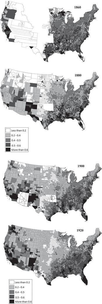
There was a great deal of variation in the Gini coefficient across locations and time. Figure 2 shows that land in farm operations was more unequally distributed in the South and West than in the Northeast and Midwest.Footnote 24 In the Midwest and Northeast, the inequality measure displayed relatively little variation, in contrast with the large degree of variation within the South and West. In fact, farm inequality in the South marches with cotton production. The Gini coefficient was higher in the cotton counties on either side of the Mississippi River and along the Atlantic coast, but lower for the non-cotton counties of Georgia and Tennessee. The finding suggests that variables such as soil quality, topography, and climate could have shaped the amount of inequality over time by altering the types of crops that could be farmed (Higgs Reference Higgs1977; Ransom and Sutch Reference Ransom and Sutch1977).
GINI COEFFICIENT BY COUNTY (1860–1920)

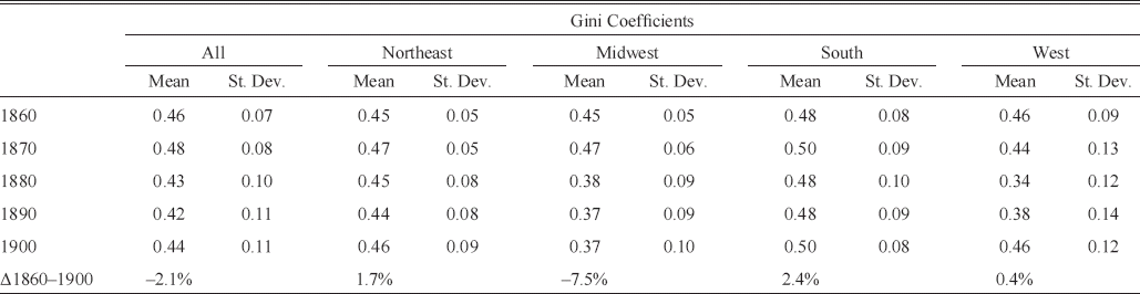
Table 1 indicates that the inequality in the size of farm operations was rising in the South and Northeast and falling in the Midwest and West. Between 1860 and 1900, inequality rose by almost 2 percentage points in the Northeast and 2.4 percentage points in the South, but declined by 2.9 percentage points in the West and 7.4 percentage points in the Midwest. Despite the release of former slaves into the southern labor market, farm size inequality only slightly increased between 1860 and 1870 and had nearly returned to its original value by 1880. This temporary increase was likely caused by the time it took freedmen to become farm operators.
TRENDS IN LAND CONCENTRATION BY REGION (1860–1900)

Note: Table presents the average Gini coefficient of each region in each year.
Sources: Gini coefficient calculated from Haines (Reference Haines2004). See text for calculation details.
In order to properly observe the relationship between inequality and banks, we need to control for the large number of characteristics and institutions that could have been driving both factors. We, therefore, proceed with a regression analysis at the county-level aggregated up to their 1860 boundaries. To examine local conditions of interest groups in agricultural regions rather than relationships in areas where agriculture was not important, we drop any county that was larger than 7,000 square miles as well as those that had fewer than 20 farms or a city of 25,000 people or more.Footnote 25 First, the square mile limit was imposed because the aggregation to counties based on 1860 boundaries creates a few large counties where it is inconceivable that a landowner or even a group of landowners would have had the power and self-interest to effect change over such as broad area. Moreover, the larger the county is the harder it is to get a proper measure of inequality. For example, the effect of inequality of a region is very different if all the large landowners are competing in the same market versus spread out amongst many locations where they have no local competition. By dropping the extremely large counties, we avoid this type of measurement error. The cutoff was chosen based on a relative break in the distribution county size and excludes about 1.5 percent of counties with most being located on the western frontier (e.g., California, Oregon, or Texas). Second, counties with few farmers are dropped because it is unlikely that farming in these counties was important to the local community. The cutoff was chosen to eliminate the lowest 1 percent of counties. Finally, urban areas in any year are dropped because they tended to focus on manufacturing and had many types of financial institutions. The cutoff was chosen by how the Census defines a large city. About 4.5 percent of counties were dropped, mostly in the manufacturing areas of the Northeast and eastern Midwest. The resulting panel contains information for 1870, 1880, 1890, and 1900 for 1,564 counties in 38 states.Footnote 26
Following Rajan and Ramcharan (Reference Rajan and Ramcharan2011), we estimate a county's financial development over the period using a linear model.Footnote 27 However, we take further steps in the analysis by pooling the data over time and using county fixed effects to control for time-invariant features for each county, year fixed effects to control for nation-wide shocks, and state by year fixed effects to control for state-specific shocks in each year. Each observation is a county-year. The dependent variable, Banks i,t, is the number of banks per thousand residents in county i in year t (called banks per capita).Footnote 28 The full model is as follows:

X i,t –10 is the vector of time-varying county-level controls from the prior census year described later, T is a vector of year fixed effects, S is a vector of state fixed effects, u i denotes a vector of county-level fixed effects,Footnote 29 and e i,t is the error term. The vector of county fixed effects controls for features of the county, such as nearness to rivers, coast-lines, elevation, soil quality, type of agriculture, and other factors that varied across counties but not over time. The vector of year fixed effects controls for national-level shocks to the money supply and national legislation related to excise taxes and tariffs. The vector of state fixed effects interacted with the year-fixed effects controls for differences in state policies over time. For instance, Sylla (Reference Sylla1969) and James (Reference James1976) argue that the lowering of state-specific and national minimum capital requirements increased the number of banks and decreased interest rate differentials across regions.
The key parameter estimated is β 1 the coefficient on the Gini measure from the previous census year (Gini i,t –10). We measure the Gini during the previous census year to reduce problems with simultaneity and endogeneity. The models of Philippe Aghion and Patrick Bolton (Reference Aghion and Bolton1997), Abhijit Banerjee and Andrew Newman (Reference Banerjee and Newman1991), and Galor and Joseph Zeira (Reference Galor and Zeira1993) indicate that economic inequality is shaped by credit availability. In our context, the Gini in year t would likely have been influenced by Banks in year t, leading to a correlation with the error term e i,t. The Ordinary Least Squares (OLS) estimation of Banks i,t on Gini i,t thus would lead to a bias to the extent that increases in the financial development affected inequality. Because serial correlation in most economic series rarely extends beyond five years, it is not likely that the farm inequality Gini from ten years earlier would be correlated with the error term in year t in the bank equation (e i,t).
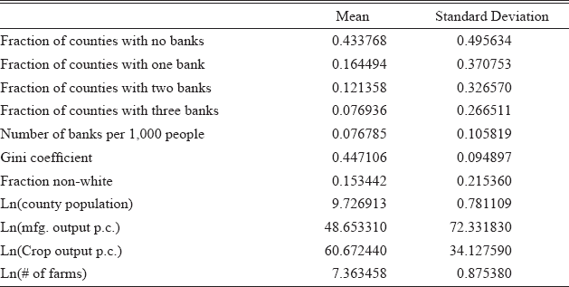
We work to eliminate any additional endogeneity bias that might arise from the omission of variables that were correlated with both banks and farm inequality. First, we control for time varying county demographics. The demand for banking services is captured by the logarithm of population, and the impact of race on credit, social, and economic relationships is captured by the fraction of the county's population that was non-white. Second, we control for the economic environment. County production is measured as the logarithms of crop output per capita and manufacturing output per capita. The size of the agricultural sector is the logarithm of the number of farms. Because the presence of a bank has been shown to lead to future growth in output and population, we use the lagged values of the county-level variables to avoid simultaneity and endogeneity. The summary statistics of the variables are presented in Table 2.
SUMMARY STATISTICS FOR 1870, 1880, 1890, AND 1900

Notes: Table presents the summary statistics of the county-level panel used in panel regressions from 1870 through 1900.
Sources: See text for data sources.
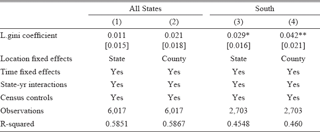
In Table 3 we present the results. The coefficients on the lagged Gini coefficient are positive, but statistically insignificant for the entire country. Because agricultural wealth was not an important driver of institutions in many areas of the country, the estimates are not unexpected. We separately estimate the model for just the southern states to see if the effects differ because most stories of powerful landlords and merchants are centered on the South. For this region, the positive effect of the Gini is statistically significant and is twice the size as the effect for all states. The evidence thus indicates that inequality had its largest impact on banks in locations where the influence of agricultural interests would have been the largest.
REGRESSION ESTIMATES EXPLAINING NUMBER OF BANKS PER 1,000 PEOPLE WITH A PANEL FOR 1870, 1880, 1890, AND 1900

* = Significant at the 10 percent level.
** = Significant at the 5 percent level.
*** = Significant at the 1 percent level.
Notes: The table presents individual linear regressions. The dependent variable is the number of banks per 1,000 people. Panel formed by aggregating counties to boundaries in 1860. Based on the Census designations, the South region defined by Alabama, Arkansas, Delaware, Florida, Georgia, Kentucky, Louisiana, Maryland, Mississippi, North and South Carolina, Oklahoma, Tennessee, Texas, Virginia, and West Virginia. County-level lagged variables: ln (population), fraction non-white, ln (manufacturing output per capita), ln (agricultural output per capita), ln (# of farms). Counties with more than 7,000 square miles, fewer than 20 farms, or any city of 25,000 or more are dropped. Dollar values are deflated to 1860 using Officer (Reference Officer2008). Robust standard are provided in brackets.
Sources: See text for data sources.
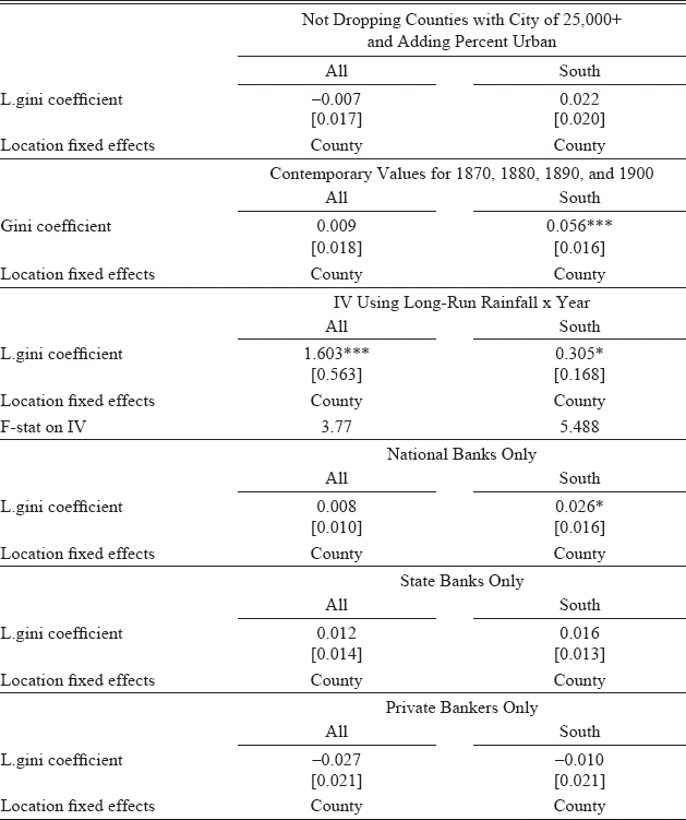
Additional specifications are reported in Table 4 to test whether the positive relationship between banks and land concentration is the result of choices about the sample and/or the inclusion of different sets or correlates. First, dropping counties with large cities helps us eliminate measurement error from locations with non-agricultural wealth and few farms. We, therefore, re-estimate equation (1) including large cities and adding a control for the fraction of people living in an urban area on the right hand side. When urban areas are included, the coefficient on the Gini in the first panel of Table 4 decreases in value and losses its statistical significance in the South. The results provide additional evidence that including areas where agricultural interests played less of a role leads to a more negative relationship between farm inequality and banks that is statistically insignificant.
IMPACT OF FARM INEQUALITY ON THE NUMBER OF BANKS PER 1,000 PEOPLE WITH ALTERNATIVE SPECIFICATIONS AND SAMPLES

* = Significant at the 10 percent level.
** = Significant at the 5 percent level.
*** = Significant at the 1 percent level.
Notes: The table presents robustness checks on individual linear regressions. The dependent variable is the number of banks per 1,000. All specifications contain county-level lagged variables: ln(population), percent black, ln(manufacturing output per capita), ln(agricultural output per capita), ln(# of farms). All specifications contain county-fixed effects, time fixed effects and the interaction between state fixed effects and time fixed effects. See text for sample composition and region definitions. Counties with more than 7,000 square miles, fewer than 20 farms, or any city of 25,000 or more are dropped. Dollar values are deflated to 1860 using Officer (Reference Officer2008). Robust standard are provided in brackets.
Sources: See text for data sources.
Using lagged values avoids the potential for auto-correlation with the error term, but could also be diluting the results. We, therefore, re-estimate equation (1) using contemporary values for all county-level variables to make sure that the results are robust to our chosen specification.Footnote 30 In the second panel of Table 4, the results using the county variables in the same year are roughly equivalent to those using lagged values in Table 3, suggesting that the results are not driven by our choice of model specification.
We take the additional step of using an Instrumental Variables estimation (IV) procedure in case the use of lagged values for the Gini does not resolve the endogeneity problem. The IV is based on the average rainfall instrument used by Rajan and Ramcharan. The presence of county-fixed effects prevents us from using long-run rainfall as the instrument and the lack of sufficient weather stations before 1896 prevents us from using rainfall per decade. In the third panel of Table 4 we interact the long-run average rainfall for 1896 to 1930 with a dummy for 1880, 1890, and 1900 to allow for variations in the effect of the rainfall on the Gini in each of the four years. Though the IV estimates likely suffer from weak instrument bias with F-statistics of 3.77 and 5.49, the IV approach produces larger coefficients than those in the OLS model. In this case, the coefficient on the Gini is positive and statistically significant for the entire nation as well as the South.
The fourth and fifth specifications are separate models with the number of state banks per thousand people and the number of national banks per thousand as dependent variables.Footnote 31 As national banks could not provide loans on real estate directly, they would have served a different purpose in agricultural regions than did state banks and would not have competed with large landowners in the provision of farm mortgage loans; therefore, the relationship between the number of banks and inequality could have been different for the two types of banks. The overall results show a positive relationship between inequality and the number of banks of any kind. While the coefficients are always positive, the relationship with inequality is only statistically significant for national banks in the South.
The final specification examines the effect of the Gini coefficient on the number of private bankers per thousand people. As previously highlighted, private bankers were unincorporated and generally were not subject to state or national regulations. They typically had little to no formal capital stock and only provided short-term consumption loans to farmers. We have not included these institutions in prior specifications because we wanted to focus on incorporated commercial banks as did Rajan and Ramcharan for 1920 and 1930. However, analyzing the relationship between private bankers and the Gini coefficient gives a sense of how land concentration affected the unincorporated banking sector. While statistically insignificant, the negative coefficients suggest a different relationship between the Gini and the number of private bankers from the ones for either national or state banks.Footnote 32 Land concentration, therefore, may have led to more incorporated banks and fewer unincorporated ones. Areas with high land concentration seem to have had commercial banks whereas those with low concentration relied more on private bankers.
WHY DO OUR RESULTS CONFLICT WITH RAJAN AND RAMCHARAM'S RESULTS FOR 1920 AND 1930
The positive relationship between banking and farm operation inequality in the late nineteenth century contrasts with the negative relationship found by Rajan and Ramcharan (Reference Rajan and Ramcharan2011) for 1920 and 1930. There are two non-mutually exclusive reasons why the results in our article differ from theirs: time period and identification strategy.
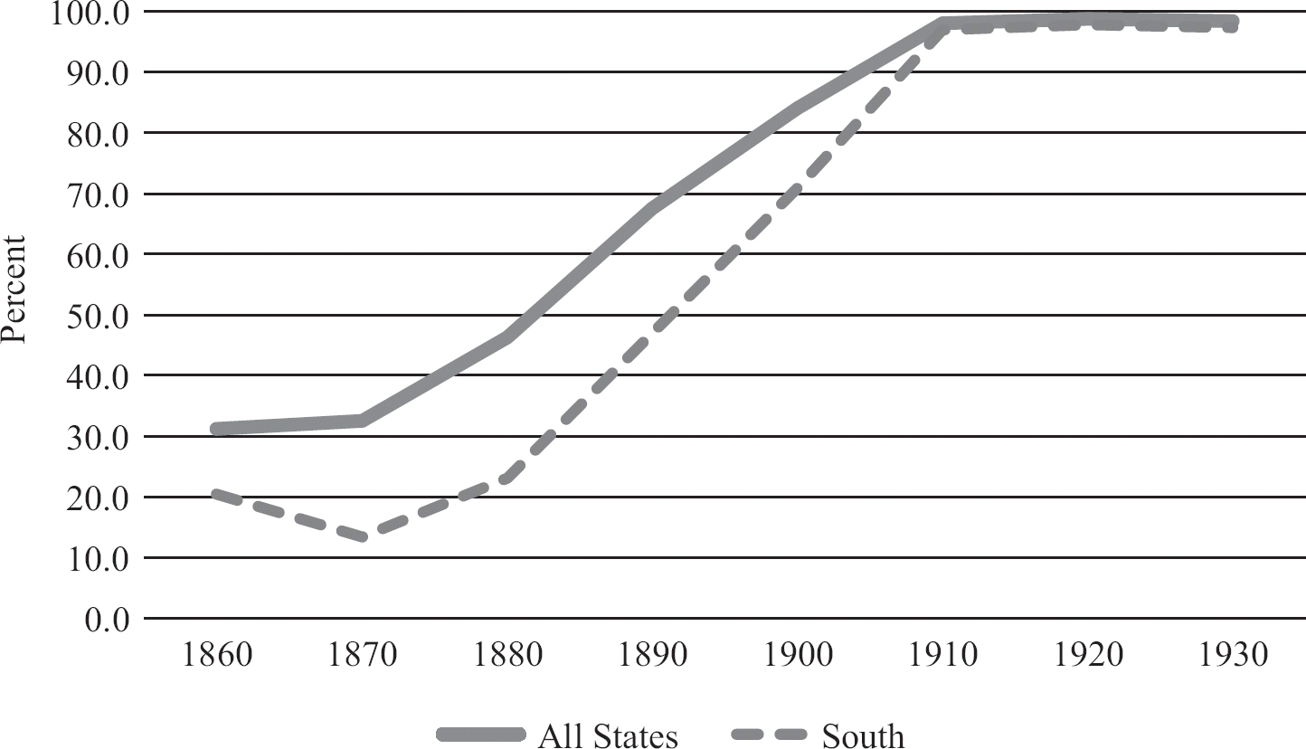
There was a substantial transformation of the financial system between 1870 and 1920. The rural banking system essentially started from scratch after the Civil War and the National Banking Acts, and the commercial banking structure was significantly more mature in 1920. As seen in Figure 3, only 32 percent of counties had at least one bank in 1870, yet more than 95 percent of counties had at least one bank by 1910 and most had multiple banks competing for business. Many of these new banks were owned by former private bankers who had operated in areas without commercial banks (Barnett Reference Barnett1911). Towards the end of the 1880s and more strongly after 1900, states explicitly attempted to stamp out private bankers by preventing them from using the word “bank” in the name as well as making them subject to state supervision and minimum capital requirements. Thus, after 1900 banks were often competing against other banks for business within the same county.
PERCENT OF COUNTIES WITH AT LEAST ONE BANK (1860–1930)

The competition for agricultural loans intensified when the federal government provided startup money for Federal Land Banks and joint stock banks after 1916. Both types of banks were created to provide funding for low interest loans to farmers.Footnote 33 Moreover, the creation of the Federal Reserve in 1914 lowered liquidity risk as it allowed member banks to borrow at the discount window to meet seasonal demand, and non-member banks often received seasonal funds indirectly through their correspondents (Calomiris, Jaremski, Park, et al. Reference Calomiris, Jaremski and Park2015). By the 1920s, the financial sector was more like that of the retailing and industrial sectors where incumbents often battled against entry by new stores. This view is consistent with Rajan and Ramcharan's (Reference Rajan and Ramcharan2016) argument that after the Great Contraction from 1929–1933 surviving banks were able to prevent new banks from rising up to take the place of those that closed.
In the 1920s farmers and farm workers had higher incomes and greater flexibility than in the late nineteenth century. For instance, 31 percent of farms had automobiles in 1920. By 1930, 58 percent of farms, 86 percent of farm owners and 48 percent of farm tenants reported having automobiles and more than 34 percent of all households reported having telephones (U.S. Census Bureau Reference Bureau of the Census1922, p. 22; 1933, p. 535; 1943, pp. 451–54).Footnote 34 Farmers, therefore, had greater capacity to go outside their community for loans, creating more cross-county competition among banks. Admittedly, this effect was probably strongest in locations where towns were clustered or in suburbs of large cities. At the same time, increased competition led to more integration of lending markets. Howard Bodenhorn's (Reference Bodenhorn, Bordo and Sylla1996) estimates show that the standard deviation across states in commercial bank interest rates fell from an average of about 5 percentage points in the late 1870s to around 2.7 in the 1890s to around 1 percentage point in the 1920s.
The difference between Rajan and Ramcharan's and our study could also be based on different identification strategies. Our panel analysis identifies the effect of the Gini coefficient based on variation over time within a county while controlling for state-wide shocks in each year. In contrast, the identification in Rajan and Ramcharam's analysis comes from variation across counties within the same state in the same year. Our panel process allows us a longer timespan to better control for omitted variable bias, whereas the Rajan and Ramcharan use an IV to reduce endogeneity and measurement error.
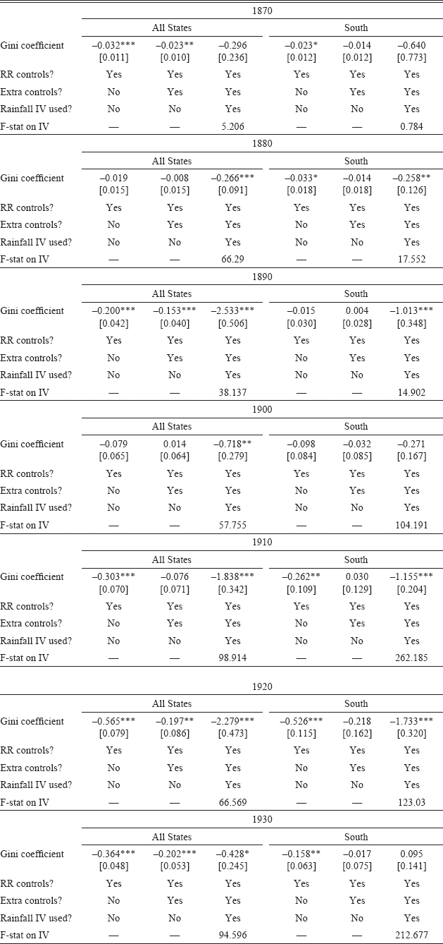
To sort out the reasons why the results differ, we have to determine whether the cross-sectional regressions tend to provide negative results in all periods and whether the additional panel controls lead to a different result in the 1900s. Adding data for 1910, 1920, and 1930, we conduct this analysis in two steps. We first examine decade cross-sections to see if the difference has to do with the additional controls and identification of the panel. We then re-estimate the panel regressions using additional years, but holding the specification fixed in order to see if the changing time-span is responsible.
We present the regression estimates in Table 5 where we apply Rajan and Ramcharam's cross-sectional approach for each decade from 1870 through 1930. Lacking time-series variation, the model is:

CROSS-SECTIONAL REGRESSION ESTIMATES EXPLAINING NUMBER OF BANKS (1870–1930)

* = Significant at the 10 percent level.
** = Significant at the 5 percent level.
*** = Significant at the 1 percent level.
Notes: The table presents individual decade cross-sectional regressions. The column headings provide the year. RR controls: population, land area, whether the county was on a large river or coast, fraction illiterate, fraction young, and fraction non-white, and state-fixed effects. Extra Controls ln (manufacturing output per capita), ln (agricultural output per capita), ln (# of farms), fraction tenants, average rainfall, average temperature, and the standard deviation of temperature, maximum change in elevation, soil moisture, percent of clay in the soil. Counties with more than 7,000 square miles, fewer than 20 farms, or any city of 25,000 or more are dropped. Dollar values are deflated to 1860 using Officer (Reference Officer2008). Robust standard are provided in brackets.
Sources: See text for data sources.
The variables retain the previous definitions with the exception of X i. Because the specifications cannot include county-fixed effects, we include a variety of constant county-level characteristics that could be driving the number of banks in X i: the fraction of the population that was illiterate, the fraction of the population that was aged 8 through 20, and the fraction of farms that are worked by a tenant.Footnote 35 It is particularly important to include the fraction of tenant farms in the county in order to control for potential mismeasurement of the Gini in locations with high shares of tenants and croppers. Because small family farms often did not generate sufficient surplus to avoid foreclosure during bad periods, we would expect locations with low rainfall and extreme temperatures naturally to have a higher concentration of acres in large farms more able to withstand shocks. Due to the lack of early weather stations, we use average rainfall, average temperature, and the standard deviation of temperature from 1895 through 1930.Footnote 36 As a rugged landscape, lack of water, and bad soil would limit agriculture, we control for the difference between the highest and lowest elevations in a county, the amount of moisture in the soil, the percent of clay in the soil, and whether the county had a large river or coast within its borders.Footnote 37
Rajan and Ramcharan's original models do not include all of these control variables. Therefore, to offer a clear comparison to their results, we estimate a regression as close to their specification as possible and then slowly add controls. We start with a model similar to theirs that only contains population, land area, whether the county was on a large river or coast, fraction illiterate, fraction young, fraction non-white, and state-fixed effects.Footnote 38 Next we add the additional census, weather, and topological controls listed earlier. Finally we follow Rajan and Ramcharan and use long-term rainfall as an instrument rather than as a control.
The identification of the impact of the Gini in Table 5 comes from variation across counties within the same state. Looking across the entire nation, the OLS results in 1920 and 1930 are similar to those Rajan and Ramcharan (Reference Rajan and Ramcharan2016) report in their Online Data Appendix. In both years the OLS coefficients for the Gini are negative and statistically significant. As we move earlier in time, however, the negative effect of the Gini becomes less stable, particularly when the additional controls are added. For instance, the coefficients in the OLS model with additional controls are not statistically significant in 1880, 1900, and 1910.
The IV strategy generally leads to a much stronger negative and statistically significant effect of the Gini coefficient on banks than do the OLS estimates. Indeed, the negative relationship is only statistically insignificant in 1870. It is not clear, however, that long-run rainfall is a good instrument in this context. The problem is not with strength, as the F-statistics for the instrument in the first stage are more than 30 in all years except for 1870, when it is 5.2. The problem is with rainfall's excludability: Can we legitimately expect that long-run average rainfall is uncorrelated with the error term? In agricultural areas, access to rainfall is a major consideration in determining economic opportunities; therefore, people considering organizing a bank were likely to consider long-run rainfall patterns when choosing to enter or exit the county. This would be true even while controlling for current or past income in the equation because long-run rainfall covers a much longer time span than just the current year. Whether the current year income was low or high, the long-run rainfall average provides additional information about whether the current year income was a good, bad, or average year. Thus, we might expect that the rainfall measure would belong in the final stage equation as a correlate. In fact, in the OLS cross-sectional analysis with long-run rainfall included as an additional correlate for banks per capita, the rainfall coefficient is negative and statistically significant in every year from 1870 to 1920. The only year in which it is not statistically significant is 1930.
As before, we estimate the cross-sectional models using only counties in the South and find much less negative results. The negative coefficients on the Gini are never statistically significant for southern counties when we include the full set of controls. Moreover, the coefficients from IV regressions are generally smaller in magnitude and are not statistically significant in 1870, 1890, 1900, and 1930. The F-statistics suggest that rainfall is not a powerful instrument of the Gini coefficient in the South until the 1900s.
The cross-sectional results suggest three conclusions. First, the differences in identification strategies lead to different results. Negative coefficients are present when the identification comes from cross-county variation within states, positive coefficients are more common when using variation across time within counties controlling for annual shocks within states. Second, the changing nature of the financial infrastructure also seems to be a factor. Specifically, the negative coefficients on the Gini are larger and more consistently significant after 1900. Third, the mix of agriculture and manufacturing areas in the nation-wide sample biases the results downwards. When focusing on the South and controlling for additional county characteristics, the negative effect of the Gini is never statistically significant.
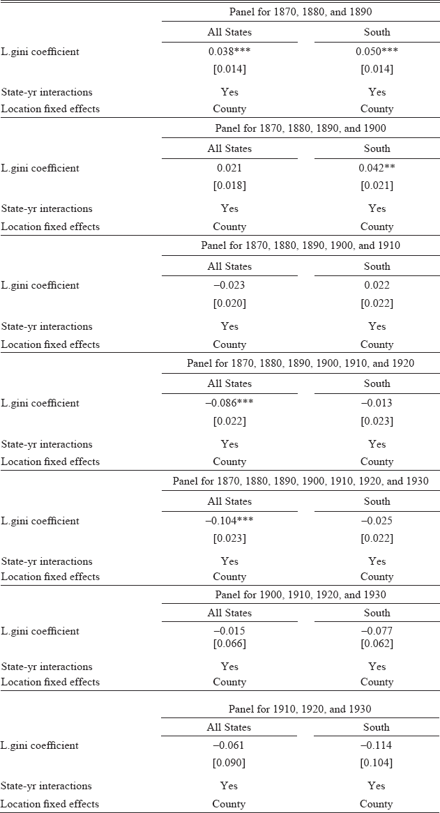
We next test whether the panel structure also picks up this change in the effect of the Gini coefficient. To do so, we extend our panel analysis through additional years. Specifically, we examine the results when adding additional data for 1910, 1920, and 1930.Footnote 39 The first panel of Table 6 shows the results when estimating equation (1) using just 1870 through 1890. Then each subsequent panel adds another decade. Like Rajan and Ramcharam, we control for differences in state regulation of capital, reserve requirements, usury rates, and bank supervision which in the panel context means including state-by-year fixed effects.
EXTENDING PANEL REGRESSIONS FORWARD IN TIME

* = Significant at the 10 percent level.
** = Significant at the 5 percent level.
*** = Significant at the 1 percent level.
Notes: The table presents individual linear regressions. The column headings provide the panel years. All specifications contain county-level lagged variables: ln (population), fraction non-white ln(manufacturing output per capita), ln (agricultural output per capita), ln (# of farms). All specifications contain county-fixed effects, time fixed effects and the interaction between state fixed effects and time fixed effects. See text for sample composition and region definitions. Counties with more than 7,000 square miles, fewer than 20 farms, or any city of 25,000 or more are dropped. Dollar values are deflated to 1860 using Officer (Reference Officer2008). Robust standard are provided in brackets.
Sources: See text for data sources.
In the panels for different time periods, the positive effects of the Gini coefficient are largest for the 1870–1890 and 1870–1900 periods when there were relatively few banks. The coefficients get smaller as more years are added to the panel. The coefficient on the Gini coefficient is statistically significant and positive for the entire country from 1870 through 1890. The coefficients for the full country become statistically insignificant when 1900 is added to the panel, turn insignificant and negative when 1910 is added, and become negative and significant when 1920 is added to the sample. The results for the South only sample show roughly the same pattern but with less negative coefficients. There are statistically significant positive coefficients in the panels for 1870–1890 and 1870–1900, while adding any year after 1900 leads to negative but statistically insignificant coefficients.
The comparisons of the panels suggest that there was a change in the relationship between banks and the Gini sometime after 1900. At the bottom of Table 6 are the panel results for the periods 1900–1930 and 1910–1930. The coefficients on the Gini are all negative although none are statistically significant. The changing nature of the financial system and regulation seem to be leading to a differential effect between the two time periods. Given that it is a change based on time period, it seems likely that the change would be a national one. One candidate for such a change was the new lower capital requirements in small communities for national banks enacted with the Gold Standard Act of 1900. The Act lowered the minimum capital requirement for locations with fewer than 4,000 people to only $25,000. The number of national banks grew rapidly over the next decade. Of the 3,387 national banks created between 1899 and 1909, 2,197 or 65 percent had a capital stock lower than $50,000 (Barnett Reference Barnett1911, pp. 232–33). Even as some state banks converted to a national charter, state bank growth kept pace with national banks as states further lowered their capital requirements. In particular, much of this state bank growth was driven by private bankers taking out formal bank charters as a result of new state regulations. The number of private bankers fell from around 4,300 in 1900 to less than 600 in 1930.Footnote 40 As such, the size of banks decreased over time and more areas were able to create multiple competing banks. Since most counties had a bank by 1900, it would not be a surprise that the banking elite sought to block entry, just as would be the case of any type of firm.
CONCLUSION
We examine the extent to which landed elites affected the development of commercial banking in rural areas following the Civil War from 1870 through 1900. The National Banking Acts during the Civil War forced the commercial banking system in agricultural areas to start anew. We thus examine a period near the height of landowner power, informal farm credit, and during the rebirth of agricultural finance. We find that areas with a higher concentration of farming in larger farm operations, tended to establish more banks.
The results for 1870 to 1900 differ from the finding of a negative relationship between banks and inequality by Rajan and Ramcharan (Reference Rajan and Ramcharan2011) for 1920 and 1930. We believe that there are two reasons for such a difference: a difference in the method of identification and a substantial change in the structure of banking. Rajan and Ramcharam's identification came from cross-sectional variation across counties within the same state, as well as the use of long-run rainfall as an instrument for inequality. When we use Rajan and Ramcharam's identification methods for the late 1800s, the banking-inequality relationship in the cross-section is often negative, as they found for 1920 and 1930. However, there are economic reasons to question the validity of the rainfall measure as an instrument as long-run rainfall is likely an important consideration for the decision to open a bank and likely belongs as a correlated in the final stage bank equation. In fact, it has a statistically significant effect when included alongside the Gini coefficient in the final banking equation. Our identification method is based on variation across time within counties while controlling for state-year specific differences. Using our panel identification methods, we find that there is no longer a positive relationship between banking and inequality after 1900 in most specifications.
There are a variety of reasons why the banking structure in the United States differed substantially between the late 1800s and the 1920s. Nearly every county had a bank by 1910 and most counties had multiple banks. Moreover, the federal government had sharply reduced minimum capital requirements for national banks in small communities with the Gold Standard Act of 1900. The government even began to provide start-up funding for national land banks that made loans to mutual associations of farmers, and the Federal Reserve was created to provide seasonal liquidity to banks. Most states had also begun to force private bankers operating without a charter into the formal banking sector or out of the market. Banking markets thus were more integrated and had government support after 1900.
The new results thus tell a more complex story about the relationship between inequality and financial development. When rural and agricultural areas started from scratch in the decades after the Civil War and the National Banking Acts, the elites in those areas, composed primarily of large landowners, joined forces to invest in local banks to expand credit and the breadth of development beyond agriculture. As the formal credit markets matured and interest rate differentials declined, the relationship weakened and farm operation inequality began to affect banks negatively. As part owners of the banks, landed elites had an incentive to prevent entry, just as retailers and other local businesses had incentives to prevent entry, particularly from expanding chain stores (Rajan and Ramcharan Reference Rajan and Ramcharan2016). It, however, was not until the early 1900s when population and regulation had reached a point where most counties had banks and, thus, had incumbent banks who would seek to prevent entry of new banks. Thus, the opposition to additional banks in rural areas found by Rajan and Ramcharan was more likely to have been driven by local elites protecting banks rather than protection of informal consumption credit that banks rarely ever provided.