I. INTRODUCTION
Object/target tracking refers to the problem of using sensor measurements to determine the location, path, and characteristics of objects of interest [Reference Challa, Morelande, Mušicki and Evans1]. A sensor can be any measuring device, such as radar, sonar, camera, infrared sensor, microphone, ultrasound, or any other sensor that can be used to collect information about objects in the environment [Reference Blackman and Popoli2]. The typical objectives of target tracking are the determination of the number of objects, their identities, and their states, such as positions, velocities, and in some cases their features. There are a number of sources of uncertainty in the object tracking problem that render it a highly non-trivial task. For example, object motion is often subject to random disturbances, objects can go undetected by sensors and the number of objects in the field of view of a sensor can change randomly. The sensor measurements are subject to random noise and the number of measurements received by a sensor from one look to the next can vary and be unpredictable. Objects may be close to each other and the measurements received might not produce enough information to distinguish these objects.
In this paper, we describe an algorithm, for combining range-Doppler (RD) data from multiple sensors to perform multi-target tracking. In particular, we considered the problem of very poor azimuth resolution. In this case, more than two sensors are needed to triangulate target tracks and techniques like multilateration are needed to overcome the problem.
With respect to previous work [Reference Baruzzi, Pasculli and Martorella3], a study of a model for the sea clutter has been carried out and simulated sea clutter has been added to the simulated received signal. This has been done in order to test the robustness of the proposed algorithm in a more realistic scenario since real data is not available yet. The algorithm has also been tested in conditions of nearly constant acceleration (nCA) [Reference Bar-Shalom and Li4–Reference Ristic, Arulampalam and Gordon6] instead of the more limiting scenario of nearly constant velocity (nCV) [Reference Baruzzi, Pasculli and Martorella3].
An approach for combining RD data from multiple sensors is described in [Reference Deming, Schindler and Perlovsky7]. However, this algorithm requires a very large number of iterations, which could lead to the algorithm computational overload.
This paper is organized as follows: Section II describes the detection algorithm used to detect the targets from the RD maps of each of the sensors, Section III provides a description of the tracking algorithm. The description of the simulated signal, of the scenario and the results are shown in Section IV. Finally, conclusions are drawn in Section V and future works are discussed. The processing chain is shown in Fig. 1.
Flow chart.

II. DETECTION
Detections in the RD domain for each sensor are considered as input to the tracking system. As the information related to a detection only contains range and Doppler information (and no azimuth), the target cannot be localized in a two-dimensional (2D) spatial domain (geographical coordinates) with single-sensor information only. Therefore, at least three sensors are needed to localize the target without any ambiguities.
A) RD maps
The RD maps are obtained from the baseband (BB) signal by applying a two dimensional fast Fourier transform (2D-FFT) [Reference Petri, Moscardini, Martorella, Conti, Capria and Berizzi8]. A first FFT is taken along the columns of the matrix. Then a second set of FFTs is then taken along the slow time, that is, the total number N of sweeps. Note that N is dictated by the more stringent parameter between the desired velocity resolution and the desired coherent integration gain (Fig. 3).
B) Constant false alarm rate (CFAR) detector
In detail a cell-averaging CFAR (CA-CFAR) is used [Reference Torres-Huitzil, Cumplido-Parra and López-Estrada9]. It calculates the threshold level by estimating the level of the noise floor around the cell under test (CUT). This can be found by taking a block of cells around the CUT and calculating the average power level. To avoid corrupting this estimate with power from the CUT itself, cells immediately adjacent to the CUT are normally ignored (and referred to as “guard cells”). A target is declared present in the CUT if it is both greater than all its adjacent cells and greater than the local average power level.
C) Clustering
A clustering step is then applied in order to remove the false alarms present in the black and white (BW) map obtained after the CFAR detector as well as overcoming the missed detections. In particular, a closing operation following Matlab functions have been developed which consists of a dilation followed by an erosion (using the same structuring element for both operations). This calculates the number of connected components found and, if that number overtakes a certain threshold value, the smaller ones are removed.
III. TRACKING
A) RD tracker
A first tracking stage in the RD domain has been developed in order to eliminate most of the false alarms. We use a primary tracking stage, which can handle clutter and missed detections, by forming tracks directly in the range/range-rate domain. The tracker used in this section is the same described in the next section, where we assume a third-order motion model. The state vector is given by  $\hat z = (r,\dot r,\ddot r{)^T}$, where r and
 $\dot r$ are measured and
 $\ddot r$ is initialized with zero mean. With this assumption, we restrict the movements of potential tracks to reasonable behavior of range and corresponding range-rate.
B) Cartesian tracker
First of all an algorithm for transforming RD coordinates into Cartesian coordinates has been developed. It consists of a series of operations which are described in detail in [Reference Baruzzi, Pasculli and Martorella3].
Then a multi-target tracking (MTT) algorithm based on a Linear Kalman Filter [Reference Blackman and Popoli2, Reference Bar-Shalom and Li Kirubarajan10] that exploits the measurements in the zero-elevation plane returned by the Clustering algorithm, has been applied. Data association is then performed and the track initiation, confirmation, and cancellation are obtained using a “m out of n” logic.
The main problem of the data association is how to find which measurements correspond to which target (track). The aim of this step is to determine the origin of each measurement by associating them with the existing tracks, new tracks or declaring them to be false detections. Between all techniques, in our work the Global nearest neighbor approach is used to perform the data association. It attempts to find and to propagate the single most likely data association hypothesis at each scan.
In order to simplify the data association, a gating technique, performed for each target is currently being tracked for elimination and unlikely observation-to-track pairings, is implemented. A gate is formed around the predicted measurement and all observations that satisfy the gating relationship (fall within the gate) are considered for track update. The remaining observations that have not been gated are used to initiate potentially new tracks. In detail, an ellipsoidal gate is used since, [Reference Blackman and Popoli2], as it is suitable in the case of the global nearest-neighbor approach. Every un-associated detection (measurement) initiates a tentative track. If in the subsequent scans, a tentative track is associated with some measurements (which fall into its gate), then a tentative track is promoted to a confirmed track. Otherwise, a tentative track is deleted. A confirmed track is deleted if it is not updated by measurements over several scans or a certain period of time. A flowchart, that resume all the MTT algorithm, is represented in Fig. 2)
Tracking algorithm block diagram.
IV. SIMULATION ANALYSIS
A) Simulated signal
In order to perform the multi-sensor/multi-target tracking algorithm, a simulation of the backscattered signal from multiple targets has been developed. We simulated the BB signal (equation (1)) after the matched filter, from which the RD maps for every sensor has been evaluated. After that, we applied the detection algorithm on the maps, in order to estimate the RD coordinates of each centroid for each acquisition in time. The model of the transmit signal is a sawtooth frequency-modulated continuous wave (FMCW) [Reference Jankiraman11]. The frequency at time t within each sweep is given by f = f 0 + tα where α = B/T R is the slope of the ramp, B the signal bandwidth, T R the duration time of a sweep and f 0 the carrier frequency. In particular f 0 = 9.6 GHz, B = 300 MHz, T R = 750 μs, and the observation time is set to 0.2 s
 $$\eqalign{& {s_{bb}}[m,n] = {\rm cos}({\phi _{bb}}[m,n]),\quad n = 1, \ldots, N - 1,\cr & \quad m = 1, \ldots, M - 1}. $$
In equation (1) N is the total number of sweeps, M = T R/T S, where T S is the sample period (T S = (1/f s) = 10 μs) and
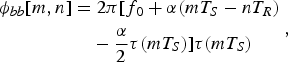 $$\eqalign{{\phi _{bb}}[m,n] & = 2\pi [{f_0} + \alpha (m{T_S} - n{T_R}) \cr & \quad - \displaystyle{\alpha \over 2}\tau (m{T_S})]\tau (m{T_S})}, $$
 $$\tau (m{T_S}) = \displaystyle{{2{R_0}} \over c} + \displaystyle{{2{v_r}} \over c}m{T_S}, $$
where R 0 is the distance of the target from the sensor at the instant t 0, v r is the radial velocity of the target, and c the speed of the light. The signal s bb[m,n] and the relative RD maps are represented in Fig. 3. The RD maps are obtained from the BB signal by applying a 2D-FFT.
Matrix of the BB signal (on the left) and relative RD map (on the right).
B) Sea clutter simulation
In this work, a simulation of a correlated K-distributed model for sea clutter is added to the received signal [Reference Xiaofei and Xiaojian12]. It combines a fast Gamma distributed random variable generation method to make the procedure much simpler. The statistics of a compound K-distributed random variable X are described by the probability density function (PDF):
 $${f_x}(x) = \displaystyle{{2c} \over {\Gamma (\nu )}}{\left( {\displaystyle{{cx} \over 2}} \right)^\nu} {K_{\nu - 1}}(cx), $$
where x > 0, Г(·) is the standard Gamma function, and K v−1(·) is the modified second-kind Bessel function of order v − 1. The K-distribution is completely specified by the shape parameter v which defines the spikiness of sea clutter and by the scale parameter c which is a positive constant related to the power characteristic of returned echo signals: the less is the value of the scale parameter, the more powerful are reflected signals from the sea surface. The shape and the scale parameters are chosen accordingly with [Reference Greco, Watts, Theodoridis and Chellappa13].
The compound K distribution can be regarded as a complex Gaussian process modulated by a process whose PDF is a generalized Chi-distribution. Let X be the K-distributed clutter, it can be expressed as the multiplication of two components as:
 $$X(k) = {X_\chi} (k){X_N}(k),$$
where X χ is a Chi-distributed random sequence, and X N is a complex Gaussian process. Since the Chi-distribution can be regarded as the square root of the Gamma distribution, the final model can be expressed as:
 $$X = \sqrt {{X_G}} {X_N}.$$
Regarding sea clutter reflectivity, a parametrized expression [Reference Gregers-Hansen and Mital14], which could be used as a basis for such a new empirical sea clutter model using the Nathanson tables as the point of reference, has been used. These tables give the value of sea clutter reflectivity as a function of frequency, grazing angle, sea state, and polarization. The proposed expression has the form:
 $$\eqalign{{\sigma _{H,V}} = & {c_1} + {c_2}\log ({\rm sin}(\alpha )) \cr & + \displaystyle{{({c_3} + {c_4}\alpha )\mathop {\log} \nolimits_{10} (f)} \over {(1 + {c_5}\alpha + {c_6}SS)}}{c_7}{(1 + SS)^{{1 \over {2 + {c_8}\alpha + {c_9}SS}}}},} $$
where α is the grazing angle (degrees), SS is the sea state, and f is the radar frequency (GHz). Using the nine parameters, c 1, c 2, …,c 9, the functional form of the equation, from which the sea clutter reflectivity can be calculated, is defined. Different sets of these nine parameters are needed for horizontal and vertical polarization, respectively [Reference Gregers-Hansen and Mital14].
An Autoregressive (AR) model of the first order has been used in order to produce a mathematical model with which the clutter signal can be generated and processed to test the detection algorithm [Reference Xiaofei and Xiaojian12]. This will help to obtain the correlated complex Gaussian process. A more accurate model of radar sea clutter will be developed by considering a higher AR model order, since the higher the order of the AR process, the more accurate the approximation will be.
C) Setup
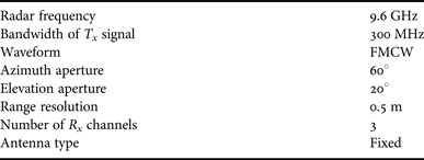
The simulated maritime scenario considered in this paper is a schematic representation of the harbor of Salerno. It is made up of four active high-resolution radars whose parameters of interest are summarized up in Table 1. The target used in the simulations, a Swerling I target model, is a ship [Reference Baruzzi, Pasculli and Martorella3], made of about 2000 scatterers. Since the radars used have high-resolution, the target will appear in more than one resolution cell. Its models for the evolution in time of the state vector have been considered as nCV and nCA. The target velocity has been randomly initialized according to the typical velocities of targets in the considered scenario, while target acceleration is initially set equal to zero. All targets are assumed to be lying on the zero-elevation plane while the radars are placed at a height of 20 m. The origin of the common Cartesian reference system is chosen to coincide with one of the four radars (in this case it was chosen to correspond with the sensor represented in cyan in Fig. 10). Then, for each sensor, we stack the target's detections in the RD domain. False alarms thermal noise and simulated sea clutter are also added to the stack of detections. It is worth mentioning that not all the targets are necessarily visible from every sensor, because of the azimuth aperture limitation. Moreover, some trajectories may be partially formed at the output of one sensor while being complete or partially formed at the output of another sensor.
Parameters of interest of each sensor.
D) Results
First of all, in Fig.s 4–7, we can see the results after the detection step that are the target estimated centroids and bounding box (in red in Figs 4 and 6).
Output from the CFAR detector with estimated centroids and bounding box.
Estimated centroids and bounding box put on top of the RD maps of each sensor.
Zoom of the output from the CFAR detector applied to the RD map of the first sensor.
Zoom of the estimated centroids and bounding box put on top of the RD map of the first sensor.
Then, the first tracking stage represented by the RD tracker, has been used to reduce the amount of false alarms randomly added before the detection step and with the same power of the received target signal. In Figs 8 and 9 two examples of the RD-tracker performance applied, respectively, to the first and third sensor are shown. We can clearly notice that the number of false alarms after this stage is much lower compared with the case where the RD tracking is not applied.
Output relative to sensor 1 from the RD tracker. In blue are represented the real measurements, and in red the estimated tracks.
Output relative to sensor 3 from the RD tracker. In blue are represented the real measurements and in red the estimated tracks.
The successive part is relative to the result of the Cartesian tracking. The results shown are obtained in two different cases: the first one when all the 2000 scatterers that form the target are considered, the second one when only half of the total number of scatterers are taken into account. The considered scatterers are selected by taking only those scatterers that lie in the space closer to the transmitter with respect to the plane passing for the target's centroid and perpendicular to the one given by the intersection between the z-axis and the line of sight that connects the transmitter and the target's centroid (Figs 11 and 12 show the scatterers of the same target seen, respectively, from the first and the second transmitter).
Results obtained by considering all the scatterers that form the target. In blue the real trajectories are shown, while the estimated tracks are represented in red.
Masked target seen by T x 1.
Masked target seen by T x 2.
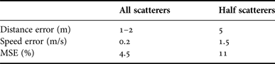
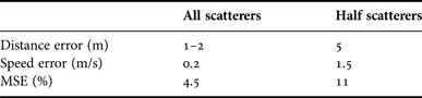
With respect to the first case, Fig. 10 shows the estimated trajectories (red lines) and the actual ones (in blue). It is possible to observe the capability of the algorithm to correctly estimate the position of the target with a mean square error (MSE) value of about 4.5%. As explained accurately in [Reference Baruzzi, Pasculli and Martorella3], during the pre-tracking stage we have to tolerate an error in terms of distance and speed due to the centroids estimation. In this case, the errors are approximately 1–2 m and 0.2 m/s. The algorithm described is also able to handle ghost targets. In fact, it is possible to see that no ghost targets appear. That proves that the algorithm is able to discriminate a real target from a ghost.
Figure 13 shows the case where only half of the 2000 scatterers are considered. Here, the same distance and speed errors as the previous case have been accepted. In Fig. 14, the errors are higher (5 m and 1.5 m/s, respectively). In this case, the algorithm performance falls down from 4.5 to 20% (Fig. 13) to 11% (Fig. 14). This is an obvious consequence of the fact that the centroid of a target seen, for example, from Tx 1 differs from the same centroid seen by another of the remaining transmitters. This error in the centroid position estimation also affects the capability of the algorithm to detect the ghost targets. The algorithm is still capable of reducing the number of ghosts but some ghosts could still persist.
Results obtained by considering only the visible scatterers that form the target. In blue the real trajectories are shown, while the estimated tracks are represented in red. Distance and speed errors are equal to 1–2 m and 0.2 m/s, respectively.
Results are obtained by considering only the visible scatterers that form the target. In blue the real trajectories are shown, while the estimated tracks are represented in red. Distance and speed errors are equal to 5 m and 1.5 m/s, respectively.
V. CONCLUSIONS
This paper presents a multi-target tracking algorithm in a multi-sensor maritime scenario when only range and Doppler information of the target are used. The algorithm has proven to be effective in simulated scenarios and performs well even with regard to the ‘deghosting’ problem and in the presence of sea clutter. The algorithm seems to be robust both for the nCV and the nCA target models for the evolution in time. Table 2 sums up the results of the simulation described in Section IVD).
Results in term of MSE and number of ghost targets.
ACKNOWLEDGEMENTS
This work has been partially funded by the Italian Ministry of University and Research (HABITAT project).
Aurora Baruzzi received her Masters degree in Telecommunication Engineering from the University of Pisa in 2011. She spent, 6 months at the University College London (UCL) in 2011, working on classification of scaled radar target data collected at ultrasound frequencies. For 2 years (2012–2014) she worked as a Research Assistance at Radar and Surveillance Systems (RaSS) National Laboratory in Pisa (Italy), laboratory of Consorzio Nazionale Interuniversitario per le Telecomunicazioni (CNIT). She is a Ph.D. student at the University of Pisa since 2012 and from March 2014 she is working at the Fraunhofer Institute für Hochfrequenzphysik und Radartechnik FHR in Wachtberg (Germany) for the passive radar and anti-jamming techniques department. Her main research interest is multi-sensors multi-targets tracking.
 Marco Martorella received his Ph.D. degree in Remote Sensing in 2003 at the University of Pisa. He is now an Associate Professor at the Department of Information Engineering of the University of Pisa and an external Professor at the University of Cape Town. He is author of about 150 international journal and conference papers, three book chapters, and a book entitled ‘Inverse Synthetic Aperture Radar Imaging: Principles, Algorithms and Applications’. He is a member of the IET Radar Sonar and Navigation Editorial Board, a senior member of the IEEE, and a member of AFCEA. He is also chair of the NATO SET-196 on ‘Multichannel/Multistatic radar imaging of non-cooperative targets’. He has been recipient of the 2008 Italy–Australia Award for young researchers, the 2010 Best Reviewer for the IEEE GRSL, and the IEEE 2013 Fred Nathanson Memorial Radar Award.