
1. Introduction
Turbulent plumes are at the core of several natural phenomena. For example, plumes are formed during volcanic eruptions, and their dynamics controls the transport of fine ash in the atmosphere (Woods Reference Woods2010). In deep oceans, water heats up during the formation of ocean crust, forming plumes which can rise up to 300 m above the sea bed (Speer & Rona Reference Speer and Rona1989). Plumes are also of central relevance in atmospheric cumulus convection (De Rooy et al. Reference De Rooy, Bechtold, Fröhlich, Hohenegger, Jonker, Mironov, Pier Siebesma, Teixeira and Yano2013), which plays a fundamental role in the weather and climate dynamic. The dynamics of plumes has been studied since the seminal, analytical work of Zeldovich (Reference Zeldovich1937), with an increasing scientific interest in the last decades, producing a vast literature thoroughly reviewed by Hunt & van den Bremer (Reference Hunt and van den Bremer2011).
Plumes are usually described as ‘lazy’, if their motion is mostly triggered by buoyancy and the initial momentum at their source is negligible, or otherwise as ‘forced’ (or buoyant jets) if their momentum cannot be neglected (Hunt & van den Bremer Reference Hunt and van den Bremer2011; van Reeuwijk & Craske Reference van Reeuwijk and Craske2015). Forced plumes become jets when buoyancy effects are negligible. By dimensional analysis, one obtains that the ratio between forced and natural convection can be represented either through the Froude number  $Fr=U/\sqrt {g H}$ or the Richardson number
 $Ri=Fr^{-2}$, where
 $U$ is the characteristic flow velocity,
 $g$ is the gravitational acceleration and
 $H$ is the characteristic flow scale (the precise definition of these quantities will be provided in § 2). Due to the relevance of entrainment quantification in these flows, also the flux-balance parameter (Morton Reference Morton1959) is often used to characterize the plume as lazy or forced, as it directly depends on the entrainment coefficient (see van Reeuwijk & Craske (Reference van Reeuwijk and Craske2015) for an exhaustive review on the subject).
Considerable effort has been devoted to the investigation of the local phenomena driving entrainment. The exchange of momentum and scalar concentration takes place across the region known as the turbulent/non-turbulent interface (TNTI), first examined by Corrsin & Kistler (Reference Corrsin and Kistler1955), whose topology determines the mixing and the growth of the turbulent region (see da Silva et al. (Reference da Silva, Hunt, Eames and Westerweel2014) for a detailed review). In this regard, the topology of the TNTI has been thoroughly studied and characterized in jets (Westerweel et al. Reference Westerweel, Fukushima, Pedersen and Hunt2005; da Silva & Taveira Reference da Silva and Taveira2010), wakes (Bisset, Hunt & Rogers Reference Bisset, Hunt and Rogers2002), turbulent boundary layers (Borrell & Jiménez Reference Borrell and Jiménez2016; Watanabe, Zhang & Nagata Reference Watanabe, Zhang and Nagata2018), shear layers (Watanabe et al. Reference Watanabe, Sakai, Nagata, Ito and Hayase2015) and other flow configurations. However, several aspects concerning the dynamics of entrainment (e.g. nibbling and engulfment processes) are still a subject of debate (Mathew & Basu Reference Mathew and Basu2002; Westerweel et al. Reference Westerweel, Fukushima, Pedersen and Hunt2009; Cimarelli & Boga Reference Cimarelli and Boga2021). Krug et al. (Reference Krug, Chung, Philip and Marusic2017) reported that the increased rate of entrainment observed in buoyant plumes, compared with pure jets, may be due to the additional contribution of the baroclinic torque and can be quantified to be of the order of 10 %–15 %.
At late times, temporal plumes will always become lazy, but it is still unclear how the transition from the forced to the lazy regime occurs. In particular, it remains to be assessed whether the two regimes can be independently observed and how the spreading evolves in the transition region. Such a transition is difficult to describe in full-scale phenomena, as the spatially evolving flow adds an intrinsic complexity. For example, a characterization was performed by Mazzino & Rosti (Reference Mazzino and Rosti2021), where the authors studied the turbulence properties of a puff (temporal jet propagating normally to buoyant forces). Another transition from the momentum-dominated to buoyancy-dominated regime has been studied within the combination of Kelvin–Helmholtz and Rayleigh–Taylor instability and mixing (Snider & Andrews Reference Snider and Andrews1994; Akula et al. Reference Akula, Suchandra, Mikhaeil and Ranjan2017), and recently investigated in the turbulent regime (Brizzolara et al. Reference Brizzolara, Mollicone, van Reeuwijk, Mazzino and Holzner2021, Reference Brizzolara, Mollicone, van Reeuwijk and Holzner2023).
A first level of simplification may be achieved considering the planar configuration. In this set-up, azimuthal symmetries are recovered in the spanwise direction. Paillat & Kaminski (Reference Paillat and Kaminski2014) study the entrainment in planar forced plumes, developing a theoretical model to describe the effect of the planar shape on entrainment. Spatial planar plumes were also mathematically characterized by van den Bremer & Hunt (Reference van den Bremer and Hunt2014a,Reference van den Bremer and Huntb), where the authors used the scale diagrams (originally presented by Morton & Middleton Reference Morton and Middleton1973) to provide solutions for several types of plumes (both lazy and forced) and jets.
The complexity due to anisotropy and inhomogeneity can be further reduced by adopting a temporally evolving set-up, better suited to study the transition from the momentum to the buoyancy-dominated regime. In this context, the planar and temporally evolving configuration allows the use of periodic boundary conditions and the recovery of the statistical homogeneity both in the streamwise and in the spanwise directions. Despite its simplification, the framework provided by temporally evolving flows allows to grasp the main flow features. As shown by Krug et al. (Reference Krug, Chung, Philip and Marusic2017) for a temporally evolving plume, this flow paradigm is comparable to the corresponding spatially evolving flow in the presence of a strong co-flow. The combination of planar and temporal configuration has been used both in pure jets (da Silva & Pereira Reference da Silva and Pereira2008; van Reeuwijk & Holzner Reference van Reeuwijk and Holzner2014; Cimarelli et al. Reference Cimarelli, Mollicone, Van Reeuwijk and De Angelis2021) and in plumes (Krug et al. Reference Krug, Chung, Philip and Marusic2017).
The present work addresses the properties of global scalings observed during the transition from forced to lazy plumes, i.e. from momentum- to buoyancy-dominated regimes. The topological and local properties of the entrainment process, thoroughly studied in the literature, are not considered here. In particular, the main focus is devoted to the characterization of the transition regime itself. To this extent, by considering an initial flow condition with a pre-imposed velocity profile of width  $H_0$, it is known that the time evolution of the width scales as
 $H(t)\propto t^{1/2}$ for the momentum-dominated regime, while
 $H(t)\propto t$ is expected for the buoyant-dominated regime. Whether these regimes can be clearly distinguished and if the transition occurs neatly or smoothly are the objects of the present work.
The remainder of this paper is organized as follows. In § 2, we present the mathematical model and the theoretical predictions together with a summary of the numerical simulations. In § 3, we discuss the numerical results, while § 4 is devoted to the conclusions.
2. Theoretical description and numerical methods
2.1. Flow settings and theoretical scaling
We consider a planar, temporal forced plume with an initial velocity and temperature fields given by  $u_x=u_y=0$ and by
 $$\begin{gather} u_z(x,y,z,t=0)= U_0\, f(x/H_0), \end{gather}$$
 $$\begin{gather}\theta(x,y,z,t=0)= T_0\, f(x/H_0), \end{gather}$$
where  $x$ is the cross-stream direction,
 $y$ is the spanwise direction,
 $z$ is the streamwise direction,
 $H_0$ is the initial width of the forced plume,
 $U_0$ is the initial velocity of the forced plume,
 $T_0$ is the difference between the temperature inside and outside the plume (which is assumed to be positive), and
 $f(\xi )$ (with
 $\xi =x/H_0$) is a symmetric, dimensionless function which has a limited support around
 $\xi =0$ such that
 $\int f(\xi ) \,{\rm d}\xi = 1$. By considering an incompressible flow and the Boussinesq approximation, the evolution of the velocity and the temperature fields is governed by
 $$\begin{gather} \frac{\partial {\boldsymbol{u}}}{\partial t} + \boldsymbol{u} \boldsymbol{\cdot} \boldsymbol{\nabla}\boldsymbol{u} +\frac{1}{\rho_0} \boldsymbol{\nabla} p - \nu \nabla^2 \boldsymbol{u} + \beta \boldsymbol{g} \theta =0, \end{gather}$$
 $$\begin{gather}\frac{\partial \theta }{\partial t} + \boldsymbol{u} \boldsymbol{\cdot} \boldsymbol{\nabla} \theta - \kappa \nabla^2 \theta = 0, \end{gather}$$
where  $\nu$ is the kinematic viscosity,
 $\kappa$ the thermal diffusivity,
 $\beta$ the thermal expansion coefficient and
 $\boldsymbol {g}=(0,0,-g)$. The dimensionless parameters which define the initial state are the Reynolds number
 $Re_0=U_0 H_0/\nu$, the Froude number
 $Fr_0=U_0/\sqrt {A_0 g H_0}$ and the Prandtl number
 $Pr = \nu / \kappa$, where
 $A_0=\beta T_0/2$ is the Atwood number. In the present work, all the simulations are done at
 $Pr =1$.
The system of equations (2.3) and (2.4) is solved in a cubic box of size  $L$ by using periodic boundary conditions and the initial conditions (2.1) and (2.2). As a consequence, the flow is statistically homogeneous in the spanwise
 $(y)$ and streamwise
 $(z)$ directions and is statistically symmetric about the
 $x=0$ plane, and the average operator (hereafter denoted as
 $\overline {({\cdot })}$) can be composed by a spatial average in the
 $y$–
 $z$ plane and by an ensemble average over independent samples. In accordance with such statistical symmetries of the flow, the equations for the mean flow solution read
 $$\begin{gather} \frac{\partial \overline{u_z} }{\partial t} = \nu \frac{\partial^2 \overline{u_z} }{\partial x^2} -\frac{\partial \overline{u_z u_x} } {\partial x} +\beta g \bar{\theta} , \end{gather}$$
 $$\begin{gather}\frac{\partial \bar{\theta} }{\partial t}= \kappa \frac{\partial^2 \bar{\theta} }{\partial x^2} -\frac{\partial \overline{\theta u_x} }{\partial x} . \end{gather}$$
Integration over  $x$ gives the equations for the total thermal content
 $C(t) \equiv \int _L \bar {\theta }(x,t)\, {{\rm d}\kern0.7pt x}\equiv C_0$ and the volume flux
 $Q(t) \equiv \int _L \overline {u_z}(x,t)\, {{\rm d}\kern0.7pt x}$, which obey
 $$\begin{gather} \frac{{\rm d} Q }{{\rm d} t} = \beta g C, \end{gather}$$
 $$\begin{gather}\frac{{\rm d} C }{{\rm d} t} = 0, \end{gather}$$
with the obvious solutions
 $$\begin{gather} Q(t)=Q_0 + \beta g C_0 t, \end{gather}$$
 $$\begin{gather}C(t) = C_0 . \end{gather}$$
Given the expressions (2.1) and (2.2) for the initial profiles, we have an explicit expression for the integration constants  $C_0=T_0 H_0$ and
 $Q_0=U_0 H_0$. Equation (2.9) indicates the presence of two different regimes in time. Initially, the constant term
 $Q_0$ dominates the flow rate: this is the shear (or jet) regime. At later times, buoyancy increases the total momentum together with the flow rate
 $Q$: this is the buoyancy (or plume) regime. The transition between the two regimes is expected to occur when the two terms in (2.9) are of the same order, i.e. at the cross-over time
 \begin{equation} t_g = \frac{U_0}{\beta g T_0}= \frac{Fr_0^2}{2} t_0, \end{equation}
where  $t_0=H_0/U_0$ is the shear time. The above relation shows that the transition time to the buoyancy regime increases quadratically with the Froude number. We remark that an equivalent cross-over time has been introduced in the case of unstably stratified shear layers by Brizzolara et al. (Reference Brizzolara, Mollicone, van Reeuwijk, Mazzino and Holzner2021).
In analogy with the initial condition, we rewrite the total thermal content and volume flux as
 $$\begin{gather} Q(t)=U(t) H_U(t), \end{gather}$$
 $$\begin{gather}C_0=T(t) H_{T}(t). \end{gather}$$
The characteristic velocity  $U(t)$ and temperature
 $T(t)$ are defined as
 $$\begin{gather} U(t) = \frac{1}{H_U(t)} \int_L \overline{u_z}(x,t)\, {{\rm d}\kern0.7pt x}, \end{gather}$$
 $$\begin{gather}T(t) = \frac{1}{H_T(t)} \int_L \bar{\theta}(x,t) \,{{\rm d}\kern0.7pt x}. \end{gather}$$
The length scales  $H_{U}(t)$ and
 $H_{T}(t)$ represent the width at time
 $t$ of the velocity and temperature profiles, respectively. Their precise definition is arbitrary, provided that is consistent with the initial value
 $H_{U}(t=0)=H_{T}(t=0)=H_0$. In § 3.1, we will adopt a definition based on the full width at half maximum of the profiles. By inserting (2.12) into (2.9), we obtain
 \begin{equation} U(t)\, H_U(t) = U_0 H_0 + 2 g A_0 H_0 t, \end{equation}
which relates the time evolution of  $H_U(t)$ and
 $U(t)$. Introducing the time-dependent Reynolds number
 $Re(t) = U(t)H_U(t)/\nu$, the exact relation (2.16) can be rewritten as
 \begin{equation} Re(t)=Re_0 \left (1 + \frac{t}{t_g} \right ). \end{equation}
To derive an explicit prediction for the growth of  $H_U(t)$, we further assume the following dimensional relation:
 \begin{equation} \frac{{\rm d}H_U(t)}{{\rm d}t}=\alpha U(t), \end{equation}
where  $\alpha$ represents the entrainment coefficient of the process. The physical motivation for this simple dimensional relation is that the growth of the width of the plume is due to the entrainment process, which is driven by the turbulent flow inside the plume. The hypothesis of self-similarity of the flow implies that the typical intensity of the turbulent velocity fluctuations is proportional to the mean velocity
 $U(t)$. It is worth noticing that, in principle, the entrainment coefficients in the momentum-dominated and buoyancy-dominated regimes could be different. As an example, two distinct values of the entrainment coefficients have been observed in unstable stratified shear layers, depending on the regime (Brizzolara et al. Reference Brizzolara, Mollicone, van Reeuwijk and Holzner2023). Nonetheless, the assumption of a single value for the entrainment coefficient in our model has the advantage to allow the derivation of explicit predictions for the time evolution of
 $H(t)$ and
 $U(t)$.
Combining the relations (2.16) and (2.18), we obtain an explicit expression for the growth of the mixing layer,
 \begin{equation} H_U(t) = H_0 \sqrt{1 + 2 \alpha \left (\frac{t}{t_0} \right ) + \frac{2\alpha}{Fr_0^2} \left (\frac{t}{t_0}\right )^2}, \end{equation}
which can be rearranged to highlight the dependence on the cross-over time,
 \begin{equation} H_U(t) = H_0 \sqrt{1 + \alpha \, Fr_0^2 \left (\frac{t}{t_g}\right) + \frac{\alpha}{2}\, Fr_0^2 \left (\frac{t}{t_g}\right )^2}. \end{equation}
Inserting (2.20) in the exact relation (2.16), we obtain a prediction for  $U(t)$:
 \begin{equation} U(t)=U_0 \frac{H_0}{H_U(t)}\left (1 + \frac{t}{t_g} \right ). \end{equation}
Moreover, inserting (2.13) into (2.10), we get  $T(t) = T_0 H_0 /H_T(t)$. Assuming the the width of the temperature profile
 $H_T(t)$ is proportional to
 $H_U(t)$, so that the ratio
 $\gamma = H_U(t)/H_T(t)$ is constant, we can exploit the model (2.20) to obtain scaling predictions for
 $H_T(t)$ and
 $T(t)$.
From (2.11), we get that, if  $Fr_0 \gg 1$, the cross-over time
 $t_g$ is much longer than the shear time
 $t_0$. In this case, from the expressions (2.19) and (2.20), it is possible to identify two different scaling regimes that follow one another over time. In the range of times
 $t_0 \ll t \ll t_g$, the constant term
 $1$ and the quadratic term
 $(\alpha /2) Fr_0^2 (t/t_g)^2$ in (2.20) can be neglected, and the evolution is dominated by the initial momentum. This leads to the following temporal scaling laws
 \begin{equation} \left.\begin{gathered} H_U(t) = \gamma H_T(t) \simeq \sqrt{2\alpha} H_0 \left({t/t_0} \right)^{1/2} \\ U(t) \simeq \frac{U_0}{\sqrt{2\alpha}} \left({t/t_0} \right)^{{-}1/2} \\ T(t) \simeq \gamma \frac{T_0}{\sqrt{2\alpha}} \left({t/t_0} \right)^{{-}1/2} \end{gathered}\right\}. \end{equation}
The scaling law for  $T(t)$ is a consequence of the constancy of
 $C(t)=C_0$.
These scaling laws are clearly transient, because the quadratic term  $(\alpha /2) Fr_0^2 (t/t_g)^2$ in (2.20) eventually becomes dominant for
 $t \gg t_g$. Therefore, at long times, we expect that the system recovers the plume regime
 \begin{equation} \left.\begin{gathered} H_U(t) = \gamma H_T(t) \simeq \sqrt{\frac{\alpha}{2}} H_g \left({t/t_g} \right) \\ U(t) \simeq \sqrt{\frac{2}{\alpha}} U_g \\ T(t) \simeq \gamma T_g \sqrt{\frac{2}{\alpha}} \left({t/t_g} \right)^{{-}1} \end{gathered}\right\}, \end{equation}
where  $H_g=H_0(U_0/U_g)=H_0 Fr_0$,
 $U_g=(A_0 g H_0)^{1/2}$ and
 $T_g=T_0(U_g/U_0) = T_0/Fr_0$, also known as free-fall quantities. We will refer to (2.22) and (2.23) as the jet and the plume temporal scaling, respectively.
We note that the model (2.20) allows to define exactly the time of the transition between these regimes by intersecting the asymptotic laws for  $H_U(t)$. The transition is expected to occur at
 $t=2t_g$, the mixing thickness and the velocity at the transition are
 \begin{equation} \left. \begin{gathered} H_U(2t_g) {}= \sqrt{1+ 4\alpha} H_0, \\ U(2t_g) {}= (3/ \sqrt{1+ 4\alpha}) U_0 . \end{gathered}\right\} \end{equation}
In addition to the prediction for the global quantities of the system  $H_{U,T}$,
 $U$ and
 $T$, the assumption of self-similarity of the turbulent flow allows to derive also dimensional scaling predictions for other statistical quantities, such as the kinetic energy dissipation rate
 $\varepsilon _\nu = \nu \langle (\partial _j u_i)^2 \rangle$ and the r.m.s. turbulent velocity fluctuations
 $u' = \sqrt {2 k/3 }$, where
 $k = \langle \frac {1}{2} |\boldsymbol {u}-\bar {\boldsymbol {u}}|^2 \rangle$ is the turbulent kinetic energy (here and in the following,
 $\langle {\cdot } \rangle$ indicates the spatial average in the region
 $|x| \leqslant H_U(t)$). From dimensional analysis, one has
 $\varepsilon _\nu (t) \simeq U(t)^3/H_U(t)$, while the scaling of velocity fluctuations
 $u'(t)$ is assumed to be proportional to that of
 $U(t)$. Combining the scaling for
 $\varepsilon _\nu$ and
 $u'$, we can also derive a prediction for the Taylor-microscale Reynolds number
 $Re_\lambda = u' \lambda /\nu = u'^2\sqrt {15/ \nu \varepsilon _\nu }$, where
 $\lambda = \sqrt {15\nu /\varepsilon _\nu } u'$ is the Taylor microscale. In the momentum-dominated regime
 $t_0 \ll t \ll t_g$, we obtain
 \begin{equation} \left.\begin{gathered} \varepsilon_\nu(t) \simeq \frac{U_0^3}{H_0} \left({t/t_0} \right)^{{-}2} \\ Re_\lambda \simeq \sqrt{Re_0} \end{gathered}\right\} \end{equation}
and in the buoyancy-dominated regime  $t \gg t_g$, we get
 \begin{equation} \left.\begin{gathered} \varepsilon_\nu(t) \simeq \frac{U_0^3}{H_0 Fr_0^4} \left({t/t_g} \right)^{{-}1} = \frac{U_g^2}{t}\\ Re_\lambda \simeq \sqrt{Re_0} \left({t/t_g} \right)^{1/2} \end{gathered}\right\}. \end{equation}
We remark that, formally, the pure jet scaling laws (2.22) can be observed only in the case of non-buoyant temporal jet ( $Fr_0=\infty$). Therefore, if the initial Froude number is
 $Fr_0 \leqslant 1$, the jet scaling cannot be observed and the scaling (2.23) holds at all times. Moreover, at finite
 $Fr_0$, we expect that the jet term
 $\alpha Fr_0^2(t/t_g)$ in (2.20) is contaminated by both the constant term
 $1$ at short times
 $t \leqslant t_0$ and by the buoyancy term
 $(\alpha /2)Fr_0^2(t/t_g)^2$ for
 $t \geqslant t_g$, thus preventing the observation of clear jet scaling regime (2.22), unless there is a large scale separation between
 $t_g$ and
 $t_0$, i.e.
 $Fr_0 \gg 1$.
2.2. Direct numerical simulations
Direct numerical simulations of (2.3) and (2.4) have been carried out in a cubic periodic domain of size  $L^3=( 2{\rm \pi} )^3$ with
 $N^3=512^3$ equally spaced gridpoints, by means of a fully parallel standard pseudo-spectral code with a 2/3 dealiasing rule. Time integration is performed using a second-order Runge–Kutta scheme, with implicit integration of linear dissipative terms. The initial conditions are given by (2.1) and (2.2) with the initial width of the forced plume fixed at
 $H_0=L/32$ and
 \begin{equation} f(\xi) = \frac{1 }{2} \left[ 1 + \tanh\left( \frac{1 - 2 |\xi| }{2 \sigma} \right) \right], \end{equation}
where  $\xi = x/H_0$ and
 $\sigma =5/56$. A uniform random noise with relative amplitude
 $0.04$ is superimposed to the velocity and temperature fields into the inner region, to trigger the initial instability.
Six different sets of simulations have been carried out, each one with 10 different realizations of the initial random perturbation to compute statistics on appropriate sample sizes. Each set is characterized by different values of  $U_0$, corresponding to different
 $Re_0$ and
 $Fr_0$, while
 $T_0$,
 $H_0$ and
 $\nu = \kappa$ are kept fixed. An additional set of simulations with
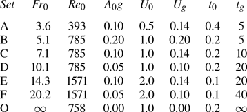
 $A_0 g=0$, corresponding to the case without buoyancy (i.e. a temporal jet with the temperature as a passive scalar) has been carried out for comparison. The complete set of parameters is listed in table 1. The characteristic scales
 $H_U$ and
 $H_T$ are computed as the full width at half maximum lengths, i.e.
 $\overline {u_z}(H_U,t) = \overline {u_z}(0,t)/2$ and
 $\bar {\theta }(H_T,t) = \bar {\theta }(0,t)/2$. This definition is consistent with the initial values
 $H_U(t=0)=H_T(t=0)=H_0$, and it has the advantage that the values of
 $H_U$ and
 $H_T$ remain constant (and equal to
 $H_0$) during the initial diffusive phase of the evolution. All the characteristic quantities reported and discussed are averaged over the 10 realizations of each set.
Parameters of the different sets of simulations, ordered with increasing  $Fr_0$. In addition to the non-dimensional parameters
 $Fr_0 = U_0/U_g$ and
 $Re_0 = U_0 H_0/\nu$, we report the numerical values (in arbitrary units) of the dimensional parameters of the simulations:
 $A_0g$,
 $U_0$,
 $U_g = \sqrt {A_0 g H_0}$,
 $t_0 = H_0/U_0$,
 $t_g=U_0/A_0 g$. The values of the other parameters are common to all simulations:
 $N= 512$,
 $L=2 {\rm \pi}$,
 $H_0=L/32$,
 $T_0 = 1$,
 $\nu =\kappa = 2.5 \times 10^{-4}$.

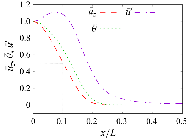
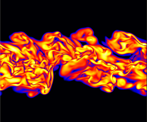
Before addressing the main results of the present work, let us introduce the main flow features by considering the flow case D. The instantaneous pattern taken by the flow is shown in figure 1 through a vertical section of the instantaneous dissipation and temperature field. A strongly convoluted shape of the plume boundaries is observed that leads to entrainment of laminar flow regions up to the very core of the jet. From a statistical point of view, the flow is characterized by profiles of vertical velocity  $\overline {u_z}(x,t)$, temperature
 $\bar {\theta }(x,t)$ and velocity fluctuations
 $\overline {u'}(x,t) = (\frac {1}{3}\overline {|\boldsymbol {u}-\bar {\boldsymbol {u}}|^2})^{1/2}$ that are shown in figure 2. A well-known bell shape is attained by the mean velocity and temperature field with turbulent fluctuations that extend significantly beyond the edge of the plume defined by the mean profile themselves.
Vertical sections in the  $x$–
 $z$ plane of (
 $a$) the dissipation field
 $\varepsilon _{\nu }$ and of (
 $b$) the temperature field from simulation D at time
 $t=25$.

Profiles of mean velocity  $\overline {u_z}$ (dashed line), temperature
 $\bar {\theta }$ (dotted line) and velocity fluctuation
 $\overline {u'}$ (dash-dotted line) for the run D at time
 $t=20$. Data are normalized using their centreline value. The black dotted line represents the extension of
 $H_U$.

We also note that the width of the temperature profile is slightly larger than that of the vertical velocity. This phenomenon is in accordance with the typical value of the turbulent Prandtl number, which is below 1 for jets and plumes (Craske, Salizzoni & van Reeuwijk Reference Craske, Salizzoni and van Reeuwijk2017).
3. Results
3.1. Time evolution of characteristic quantities
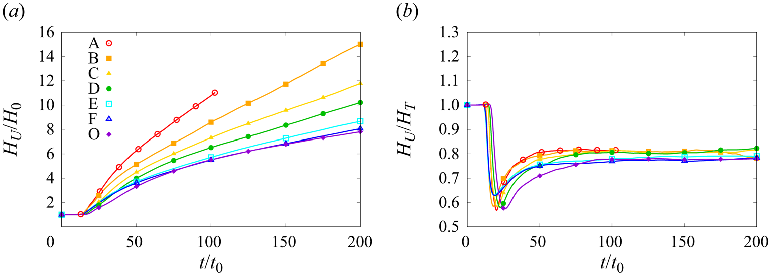
At the initial times the perturbed laminar jet displays the onset of the Kelvin–Helmholtz (KH) instability which eventually develops to a fully turbulent flow. Before the instability, the evolution of the jet is characterized by a constant width  $H_U$, as shown in figure 3(
 $a$). The duration
 $t_D$ of this initial diffusive stage (defined by the region of constant
 $H_U$) appears to be dependent on the initial Reynolds number
 $Re_0$ and we empirically find that
 $t_{D} \simeq 15 t_0$ (note that diffusivity is constant in our simulations).
( $a$) Temporal evolution of the forced plume width
 $H_U$ and (
 $b$) temporal evolution of the ratio between the velocity and temperature widths
 $H_U$ and
 $H_T$. The time is rescaled with
 $t_0$.

Figure 3( $b$) shows that in the turbulent regime, the ratio
 $H_U/H_T$ is approximatively constant (approximately
 $0.8$). For this reason, and for simplicity of the presentation, in the following, we will use
 $H_U$ as the measure of the length scale. Still, it can be observed that this ratio shows a weak dependence on the
 $Fr_0$, i.e. it is inversely proportional to it.
From figure 3( $a$), it is difficult to distinguish between the initial shear regime (2.22) and the buoyancy regime (2.23), although it is evident that the growth of the mixing layer for the three runs at the same
 $Re_0$ (A, B and C) is ordered as the inverse of
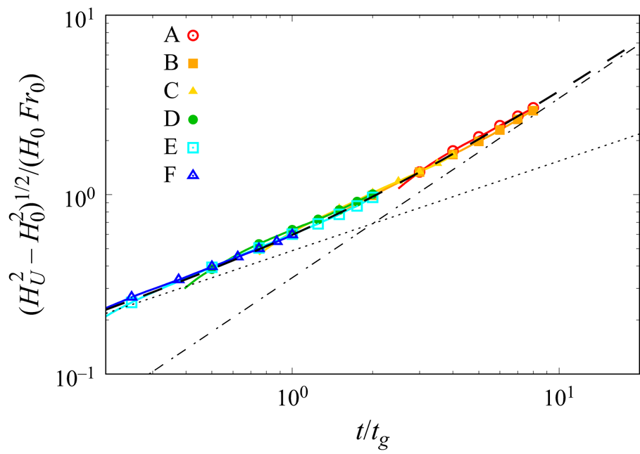
 $Fr_0$ as predicted by (2.19). Moreover, it is clear that the run O without buoyancy does not display a transition to the linear growth, typical of the plume regime. Nonetheless, the model (2.20) reproduces well the evolution of the mixing layer for all the cases considered. This is shown in figure 4, where we plot
 $(H_U^2(t)-H_0^2)/(H_0^2 Fr_0^2)$ as a function of the rescaled time
 $t/t_g$ together with the model (2.20). The value of the entrainment coefficient
 $\alpha =0.237$ has been obtained by fitting with a single curve the ensemble of data of all the simulations from A to F. The initial times (before the development of the turbulent flow) have been excluded from the fit. We remark that
 $\alpha$ is the only free parameter, as the other quantities are defined a priori and not measured.
Temporal evolution of the forced plume width rescaled according to the theoretical model (2.20). The black dashed line represents the expression (2.20) with  $\alpha =0.237$. We also show the asymptotic laws in the momentum-dominated regime (2.22) (black dotted line) and in the buoyancy-dominated regime (2.23) (black dash-dotted line). The intersection of the two asymptotic laws occurs at
 $t/t_g=2$.

Figure 4 shows that the transition between the two asymptotic regimes occurs over a broad range of time scales. Therefore, the cases considered in our study can be considered transitional cases. To fully recover the asymptotic temporal scaling  $(H_U(t)^2-H_0^2)^{1/2}/H_0Fr_0 = \sqrt {\alpha } (t/t_g)^{1/2}$ (dotted line in figure 4) of the jet regime (2.22) and
 $(H_U(t)^2-H_0^2)^{1/2}/H_oFr_0 = \sqrt {\alpha /2} (t/t_g)$ (dash-dotted line in figure 4) of the plume (2.23) regime, it would be necessary to consider cases with larger and smaller
 $Fr_0$, respectively.
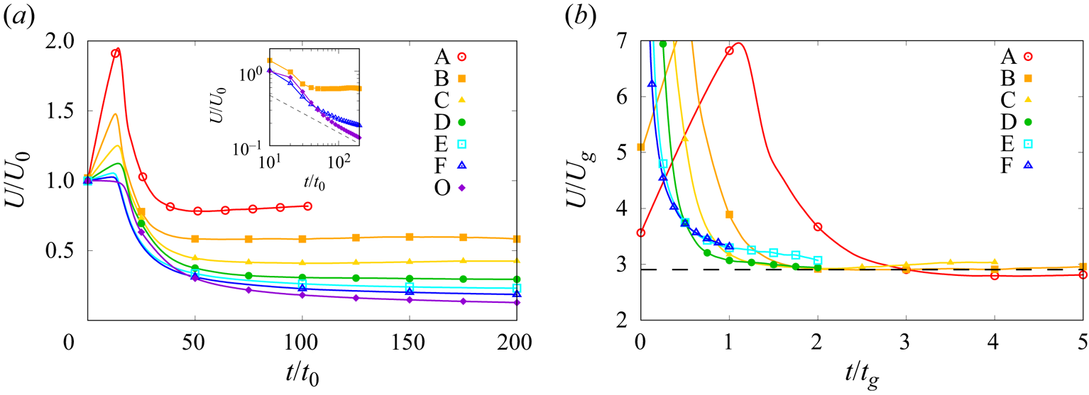
The characteristic velocity  $U(t)$ displays more clearly the transition from the jet regime (where
 $U \propto t^{-1/2}$) to the plume regime (with
 $U \sim U_g$). This is shown in figure 5(
 $a$), where we can observe that, after the initial phase corresponding to the destabilization of the initial laminar profile, the velocity amplitude reaches a constant value for all the simulations with
 $U_g>0$. In contrast, the velocity amplitude for run O (i.e. in the absence of buoyancy forces) does not reach a finite asymptotic value. These two different behaviours are even more clearly discernible in the inset of figure 5(
 $a$), where the same quantity is shown in logarithmic scale together with the jet scaling in (2.22). The case O approaches asymptotically the jet scaling
 $U(t) \simeq t^{-1/2}$, while the case B clearly shows the plateau with constant value of
 $U$. The case F (with large but finite
 $Fr_0$) is initially similar to case O, but at long times, it begins to display a convergence towards a finite value. Velocity amplitudes rescaled with the theoretical predictions (2.23) are shown in figure 5(
 $b$). In all cases, the characteristic velocity rescaled with
 $U_g$ approaches, at
 $t \gg t_g$, a constant value, which is in quantitative agreement with the prediction
 $U/U_g = \sqrt {2/\alpha } \simeq 2.9$ discussed in § 2. We remind that the value of
 $\alpha$ (which fixes the asymptotic value of
 $U/U_g$) depends on the specific definition of the amplitude
 $H_U(t)$. We note also that the rescaling of times
 $t/t_g$ is not perfect because of the presence of the initial diffusive regime that causes an initial offset
 $t_D$, which is not proportional to
 $t_g$. A better collapse of the curves can be obtained by subtracting
 $t_D$.
( $a$) Characteristic streamwise velocity amplitude
 $U$ as a function of
 $t/t_0$. The inset shows cases C, F and O on log-log axis, with a dashed line showing the power-law
 $U \sim t^{-1/2}$. (
 $b$) Scaled values of
 $U$ by free-fall velocity
 $U_g$ as a function of
 $t/t_g$. Dashed line represents the asymptotic prediction
 $U/U_g = \sqrt {2/\alpha }$.

The deviation observed at short times for the case A deserves some comments. In this case, due to the low initial values of  $Re_0$ and
 $Fr_0$, the flow accelerates much more than the other cases before developing a turbulent behaviour. This results in a maximum velocity which is approximately twice as large as its initial value, as shown in figure 5(
 $a$), and in a longer time for reaching the asymptotic value. Indeed, better collapse can be obtained by defining the buoyancy time
 $t_g$ with this maximum velocity instead of
 $U_0$.
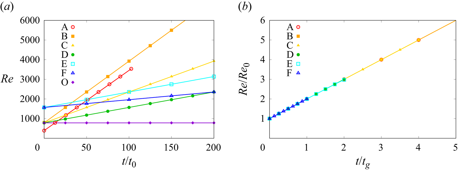
The evolution of the Reynolds number of the flow, defined as  $Re(t)=U H_U/\nu$, is shown in figure 6. We see that in all runs with finite
 $Fr_0$, it increases with time, while for run O, it remains constant. As discussed in § 2, this is a simple consequence of the fact that
 $Re(t)=Q(t)/\nu$ and of (2.9). By rescaling the time with
 $t_g$ and the values of
 $Re(t)$ with their initial value
 $Re_0$, the exact relation (2.17) is very well verified in our simulations as shown in figure 6(
 $b$).
Reynolds number  $Re (t) = U H_U/\nu$ as a function of time
 $t/t0$. (
 $a$) Unscaled values. (
 $b$) Scaled values
 $Re/Re_0$ as a function of
 $t/t_g$.

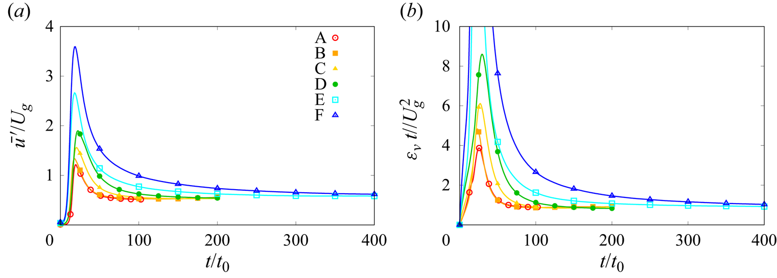
Finally, we consider the time evolution of turbulent quantities. As discussed in § 2, the r.m.s. turbulent velocity fluctuations,  $u' = \langle \frac {1}{3} |\bar {\boldsymbol {u}}-\bar {\boldsymbol {u}}|^2 \rangle ^{1/2}$, are expected to scale in time as the characteristic velocity
 $U(t)$ and, therefore, to reach an asymptotic constant value in the plume regime. Of course, at variance with the characteristic velocity, fluctuations are zero during the initial laminar phase. As shown in figure 7(
 $a$), the convergence towards an asymptotic value is observed for all the runs. At long times, the relative intensity of turbulent fluctuations
 $u'/U$ approaches a constant value
 $u'/U \simeq 0.18$.
( $a$) Amplitude of velocity fluctuations
 $u'$ rescaled with
 $U_g$ as a function of
 $t/t_0$. (
 $b$) Kinetic energy dissipation rate
 $\varepsilon _\nu$ compensated with the prediction
 $U_g^2/t$ (2.26) as a function of
 $t/t_0$.

Average energy dissipation  $\varepsilon _{\nu } = \nu \langle ( \partial _i u_j )^2 \rangle$ is plotted in figure 7(
 $b$), compensated with the dimensional scaling
 $\varepsilon _{\nu } \propto U_g^2 t^{-1}$ expected for the buoyancy-dominated regime (2.26). As for velocity fluctuations, also in this case, we observe the presence of a peak in correspondence with the development of turbulence. When comparing with figure 3(
 $b$), we see that this peak appears at the time at which the evolution of the flow enters the self-similar regime.
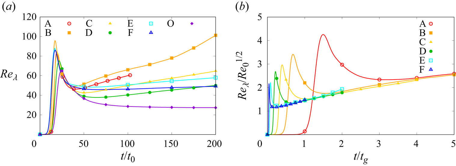
From the values of  $u'$ and
 $\varepsilon _\nu$, it is straightforward to obtain the evolution of the Taylor-microscale Reynolds number
 $Re_\lambda =u'^2\sqrt {15/ \nu \varepsilon _\nu }$, which is shown in figure 8(
 $a$). After the initial diffusive stage, in which
 $Re_\lambda$ is zero, we observe a rapid increase of the value of
 $Re_\lambda$ up to a peak value which is achieved at almost the same time as the maximum of
 $u'$ observed in figure 7(
 $a$). In the simulation with
 $Fr_0 = \infty$ (case O),
 $Re_\lambda$ attains asymptotically a constant value, in agreement with the jet-scaling prediction (2.25). A plateau corresponding to the jet scaling regime is also observed at intermediate times
 $50 t_0 \lesssim t \lesssim 150 t_0$ in the simulation with the largest (finite)
 $Fr_0$ (case F). In all the other cases (A–E),
 $Re_\lambda$ grows in time in the turbulent regime. The convergence towards the asymptotic buoyancy-dominated regime is shown in figure 7(
 $b$), in which the rescaled values
 $Re_\lambda /Re_0^{1/2}$ are plotted as a function of
 $t/t_g$, according to (2.26).
Taylor-microscale Reynolds number as a function of  $t/t0$. (
 $a$) Unscaled values. (
 $b$) Scaled values by the initial Reynolds number
 $Re_0$, as a function of
 $t/t_g$.

3.2. Velocity and temperature profiles
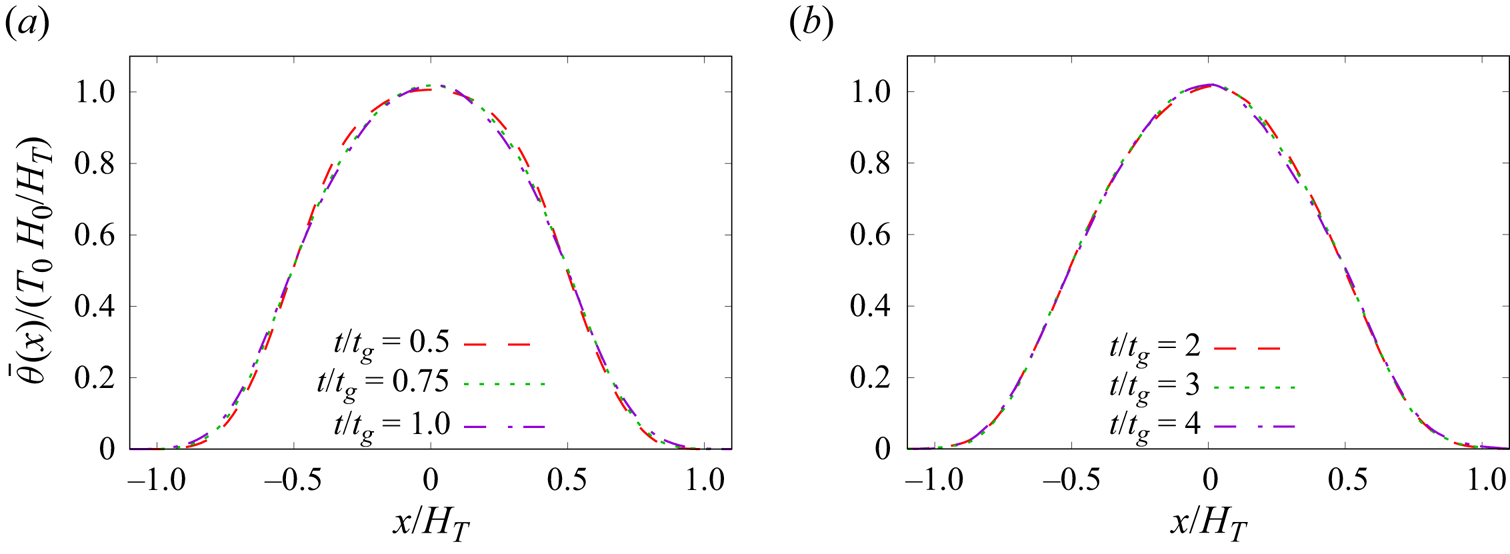
We now consider the mean velocity and temperature profiles. Since the total thermal content  $C(t) = T(t)H(t)$ is a conserved quantity in both the shear-dominated and buoyancy-dominated regimes, we expect that the mean temperature profiles
 $\bar {\theta }(x,t)$ at different times can be simply rescaled by
 $H_T(t)$ and the product
 $T_0 H_0$. Figure 9 confirms this hypothesis, indicating a remarkable self-similar behaviour of the temperature profiles, with almost no differences between the two regimes.
Mean temperature profiles  $\bar {\theta }(x,t)$ for the set C of simulations, at different times, in the (
 $a$) shear- and (
 $b$) buoyancy-dominated regimes, rescaled by the initial total thermal content
 $C_0 = T_0 H_0$ and the characteristic width
 $H_T(t)$.

Based on the hypothesis of self-similarity of the flow, we expect that also the profiles of the vertical component of the velocity  $\overline {u_z}(x,t)$ can be collapsed at all times by rescaling them with the scale
 $H_U(t)$ and characteristic velocity
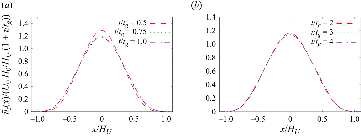
 $U(t)$ obtained from the model (2.20) and (2.21) discussed in § 2. In figure 10, we show the rescaled profiles at different times in the shear-dominated regime for the set D of simulations (panel
 $a$) and in the buoyancy-dominated regime for the set B of simulations (panel
 $b$). In almost all cases,we observe a good collapse to a self-similar profile. Note that, here, we used the same value of the parameter
 $\alpha =0.237$ which has been previously determined by fitting the time evolution of
 $H_U(t)$; therefore, the collapse of the profiles is achieved without further fitting parameters. The small deviations which are observed at short times
 $t= 0.5t_g$ in the case D can be ascribed to the fact that the turbulent regime is not yet fully achieved at that time. This is consistent with figure 9(
 $b$), which shows that in the case D, the asymptotic regime of
 $Re_\lambda$ is achieved at times
 $t > 0.5t_g$. It is interesting to notice that in the buoyancy-dominated regime, analogously to the case of the passive scalar field advected by the jet, the self-similar shapes of the temperature and velocity profiles are different from each other.
Mean profiles of vertical velocity  $\overline {u_z}(x,t)$ for the set D of simulations, at different times, in the (
 $a$) shear-dominated regime and (
 $b$) for the set B of simulations in the buoyancy-dominated regime, rescaled by the characteristic width
 $H_U$ and velocity
 $U(t)$ obtained by the model (2.20) and (2.21) with
 $\alpha =0.237$.

4. Conclusions
The transition from momentum-dominated to buoyancy-dominated regime in buoyant forced plumes is studied in the present work by means of direct numerical simulation. By considering the time evolution of the total thermal content and of the volume flux, we obtain a general model for the temporal growth of the width of the plume  $H_U(t)$ (2.20) and for its characteristic velocity
 $U(t)$ (2.21), which allows to identify two different scaling regimes, separated by a cross-over time
 $t_g$. In the limit of large
 $Re$ and
 $Fr$, the model (2.20), (2.21) prescribes that for
 $t\ll t_g$, the plume dynamic should behave as a non-buoyant jet with scaling laws
 $H_U(t)\propto t^{1/2}$ and
 $U(t) \propto t^{-1/2}$, while at later times
 $t \gg t_g$, the system retrieves the plume-like behaviour with
 $H_u(t)\propto t$ and
 $U(t)\simeq \textrm {const}$. A strong point of our model is that it provides a simple, yet effective parametrization of the transition between the two regimes, with a single fitting parameter, represented by the entrainment coefficient.
The results of the numerical simulations show that our model is indeed able to capture correctly the transitional regime which is observed at finite  $Fr$ and
 $Re$. This is confirmed also by the time evolution of the velocity profiles, which can be collapsed using the characteristic scale and velocity provided by the model. We also found that the asymptotic buoyant temporal scaling laws are always retrieved at late times, while the jet-like scaling laws are not clearly observed in the simulations at finite Froude number. Indeed, buoyancy plays a crucial role in the destabilization and the growth of the plume width, also influencing its initial stage, and hence causing deviations from the pure jet behaviour. The jet behaviour is clearly observed in the non-buoyant case, thus suggesting that, in general, one needs a very large
 $Fr_0$ (i.e. large transition time
 $t_g$) to disentangle the two scaling laws in (2.20). By increasing the initial
 $Re_0$ while keeping a constant
 $Fr_0$ (e.g. decreasing
 $\nu$), it is possible to reduce the initial diffusive stage duration
 $t_D$, anticipating the transition to the turbulent regime. Nevertheless, to observe a clear jet scaling,
 $t_g/t_0 \gg 1$ is required, implying that a high
 $Re_0$ alone is not sufficient to induce a pure jet behaviour in the initial stage. This suggests a possible line of research for future works.
Funding
We acknowledge HPC CINECA for computing resources (INFN-CINECA grant no. INFN23-FieldTurb). L.P. thanks Fondazione CRT for financial support within the project 2021.0858. M.C.-E. acknowledges the financial support given by the Department of Engineering ‘Enzo Ferrari’ of the University of Modena and Reggio Emilia through the action FAR dipartimentale 2024/2025. We also thank one of the Referees for very useful remarks which helped to improve the manuscript.
Declaration of interests
The authors report no conflict of interest.