



1. Introduction
Microbial communities are strongly influenced by the environments they inhabit. For example, the growth and morphology of bacterial colonies and biofilms depend on substrate composition and rheology (Fei et al. Reference Fei, Mao, Yan, Alert, Stone, Bassler, Wingreen and Košmrlj2020; Asp et al. Reference Asp, Thanh, Minh-Tri, Danielle, Carroll, Franceski, Welch, Gopinath and Patteson2022; Faiza, Welch & Patteson Reference Faiza, Welch and Patteson2025; Gonzalez La Corte et al. Reference Gonzalez La Corte, Stevens, Cárcamo-Oyarce, Ribbeck, Wingreen and Datta2025), substrate topography controls motility and nutrient accessibility (Chang et al. Reference Chang, Fragkopoulos, Marquez, Kim, Angelini and Fernández-Nieves2015; Gu et al. Reference Gu, Chen, Song, Brasch, Henderson and Ren2016; Postek et al. Reference Postek, Staśkiewicz, Lilja and Wacław2024), and ambient fluid flows affect morphology and population dynamics (Perlekar et al. Reference Perlekar, Benzi, Nelson and Toschi2010; Pearce et al. Reference Pearce, Song, Skinner, Mok, Hartmann, Singh, Jeckel, Oishi, Drescher and Dunkel2019; Benzi et al. Reference Benzi, Nelson, Shankar, Toschi and Zhu2022). These features, in many cases, arise from a feedback loop among growth, mechanics and chemical sensing (Hallatschek et al. Reference Hallatschek, Datta, Drescher, Dunkel, Elgeti, Waclaw and Wingreen2023).
Microbial communities at or near fluid interfaces arise in a variety of culinary, industrial and environmental contexts, and present a particularly interesting case (Vaccari et al. Reference Vaccari, Molaei, Niepa, Lee, Leheny and Stebe2017). Examples include kilometre-scale algal blooms that are mixed by turbulent oceanic flows (Abraham Reference Abraham1998; Hallegraeff Reference Hallegraeff2003), centimetre-scale pellicles that facilitate kombucha fermentation (Aung & Kim Reference Aung and Kim2024) and millimetric biofilms on oil droplets that can aid in bioremediation (Vaccari et al. Reference Vaccari, Allan, Sharifi-Mood, Singh, Leheny and Stebe2015; Hickl & Juarez Reference Hickl and Juarez2022; Prasad et al. Reference Prasad2023). Experiments of yeast colonies (S. cerevisiae) growing on viscous substrates found that metabolically generated flows, which arise from depletion of dense nutrients in the bulk, can enhance nutrient transport and drive interfacial instabilities (Atis et al. Reference Atis, Weinstein, Murray and Nelson2019; Narayanasamy et al. Reference Narayanasamy, Bingham, Fadero, Bozdag, Ratcliff, Yunker and Thutupalli2025). Particle image velocimetry measurements and simulations of a hydrodynamic model show these metabolic flows manifest as a vortex ring in the bulk and a peak in the surface velocity outside of the colony. It remains, however, unclear how these flows, along with those generated by growth, connect to the colony morphology.
In the system considered by Atis et al. (Reference Atis, Weinstein, Murray and Nelson2019) – a microbial ‘droplet’ growing on the surface of a viscous fluid – growth generates tangential stresses at the surface and nutrient consumption drives bulk convection. The resulting fluid flows then feed back non-locally onto the droplet dynamics. These features place the system within the broader class of problems involving rigid or deformable objects bound to a fluid interface. A foundational example is the translation of a rigid protein through a lipid membrane immersed in a viscous fluid, originally studied by Saffman and Delbrück (Saffman & Delbrück Reference Saffman and Delbrück1975; Saffman Reference Saffman1976) and later extended by many others (Hughes, Pailthorpe & White Reference Hughes, Pailthorpe and White1981; Stone & Ajdari Reference Stone and Ajdari1998; Stone & Masoud Reference Stone and Masoud2015). These works show that accounting for viscous stresses transmitted non-locally through the bulk fluid is essential for predicting the particle mobility. The microbial system experiences analogous viscous stresses, generated not only by growth-induced motions, but also by solutal convection in the sublayer. Importantly, non-local hydrodynamic coupling fundamentally distinguishes this system from classical range expansion on rigid substrates in which the resistive force is proportional to the local cell velocity (Greenspan Reference Greenspan1976; Lowengrub et al. Reference Lowengrub, Frieboes, Jin, Chuang, Li, Macklin, Wise and Cristini2009; Weady et al. Reference Weady, Palmer, Lamson, Kim, Farhadifar and Shelley2024).
A closer analogue to the microbial system, in which the material itself deforms, is the free-boundary evolution of monolayer domains, such as surfactant-rich regions or lipid domains, which may relax under line tension, deform under electrostatic repulsion or spread due to Marangoni stresses (Stone & McConnell Reference Stone and McConnell1995; Alexander et al. Reference Alexander, Bernoff, Mann, Mann, Wintersmith and Zou2007; Manikantan & Squires Reference Manikantan and Squires2020). In more recent contexts, such motions may be driven by active processes within the monolayer domain itself, such as self-propulsion or rotation (Masoud & Shelley Reference Masoud and Shelley2014; Fei, Gu & Bishop Reference Fei, Gu and Bishop2017; Jia, Irvine & Shelley Reference Jia, Irvine and Shelley2022). These additional degrees of freedom enable a wide range of instabilities and pattern-forming behaviours (Troian, Herbolzheimer & Safran Reference Troian, Herbolzheimer and Safran1990; Lubensky & Goldstein Reference Lubensky and Goldstein1996; Matar & Craster Reference Matar and Craster2009). As in the Saffman–Delbrück system, viscous forces imparted by the sublayer significantly modify the droplet mechanics, including the growth or decay rate of boundary perturbations and the form of internal stresses, which are generically singular at the boundary.
All of the above-mentioned systems have a similar mathematical description. Typically, the bulk fluid velocity is described by a partial differential equation (PDE), such as the Stokes equations, coupled through boundary conditions to a constitutive law for the surface rheology, which may vary across domains. For domains with high degrees of symmetry, such as the disk or perturbations thereof, analytical solutions can often be found using integral transforms or eigenfunction expansions in body-fitted coordinates (Schneider, O’Neill & Brenner Reference Schneider, O’Neill and Brenner1973; Stone & McConnell Reference Stone and McConnell1995). When only integrated quantities, such as the total force or translational velocity, are desired, the Lorentz reciprocal theorem can bypass solution of the full flow field (Masoud & Stone Reference Masoud and Stone2014; Stone & Masoud Reference Stone and Masoud2015; Elfring, Leal & Squires Reference Elfring, Leal and Squires2016). For non-structured geometries, a more flexible approach is to express the solution in terms of the associated Green's function of the bulk and/or surface operators (Lubensky & Goldstein Reference Lubensky and Goldstein1996; Chakrabarti Reference Chakrabarti2000; Williams & Squire Reference Williams and Squire2004; Jia et al. Reference Jia, Irvine and Shelley2022; Askham et al. Reference Askham, Hoskins, Nekrasov and Rachh2025). Such formulations provide a generic representation of the droplet dynamics that can be simulated numerically. However, analytically determining the appropriate Green's function can be challenging. This difficulty is particularly acute in the microbial system, where metabolically generated buoyant flows induce a non-uniform body force in the bulk.
In this work, we develop and analyse a mathematical model for a microbial droplet growing, through consumption of an underlying nutrient, on the surface of a viscous fluid. Building on classical models of interfacial flows, the model takes the form of a free-boundary problem driven by three coupled components: (i) an isotropic pressure internal to the evolving droplet arising from growth; (ii) bulk fluid flow driven by this growth pressure; and (iii) buoyancy-driven flows arising from consumption of a nutrient. In § 2, we present the partial differential equations governing the full three-dimensional system. Dimensional analysis and asymptotic reduction simplifies these nonlinear equations to a set of linear PDEs. In § 3, we exploit this linearity to reformulate the model as a system of integro-differential equations defined solely on the droplet. In this formulation, several integral operators appear whose spectral properties we discuss in § 4. These properties provide a clear route to axisymmetric solutions, which we derive in § 5. Finally, in § 6, we analyse the geometric stability of these axisymmetric solutions. This analysis shows growth stabilises axisymmetric geometries, while flows induced by nutrient consumption amplify perturbations. These results offer a rigorous mechanical explanation of the morphological instabilities observed in experiments of growing yeast colonies (Atis et al. Reference Atis, Weinstein, Murray and Nelson2019) and provide a robust mathematical framework for the analysis of microbial communities growing on fluid interfaces.
Schematic of the mathematical model. A growing microbial droplet
 $\varOmega (t)$
(green) sits on the surface
 $S$
of a semi-infinite fluid volume
 $V$
(blue). As the droplet grows, it depletes dense nutrients (red circles) in the fluid which drives buoyant flows.

Figure 1. Long description
The image depicts a schematic of a mathematical model. A growing microbial droplet, colored green, sits on the surface of a semi-infinite fluid volume, colored blue. As the droplet grows, it depletes dense nutrients, represented by red circles, in the fluid, which drives buoyant flows. The droplet is labeled as Omega(t), and the surface is labeled as S. The fluid volume is labeled as V, and the direction of gravity is indicated by a large arrow labeled g pointing downward. The image illustrates the interaction between microbial growth, nutrient depletion, and fluid dynamics.
2. A mathematical model
We consider a two-dimensional microbial droplet
 $\varOmega (t) \subset S$
growing on the surface
 $S = \partial V = \{\boldsymbol{X} = (x, y, 0) \in \mathbb{R}^3\}$
of a semi-infinite volume
 $V = \{\boldsymbol{X} = (x, y, z) \in \mathbb{R}^3 : z \lt 0\}$
of a Newtonian fluid. A schematic of this configuration is shown in figure 1. As the droplet expands, it exerts forces at the fluid surface which drive bulk flows. Simultaneously, microbial nutrient consumption establishes density gradients in the underlying fluid volume which lead to buoyancy-induced flows. The variables to be determined are therefore the bulk fluid velocity
 $\boldsymbol{U} : V \to \mathbb{R}^3$
and pressure
 $P : V \to \mathbb{R}$
, the nutrient concentration
 $c : V \to \mathbb{R}$
and fluid density
 $\rho (c) : V \to \mathbb{R}$
, and the surface growth velocity
 $\boldsymbol{u} : \varOmega \to \mathbb{R}^2$
and growth pressure
 $p : \varOmega \to \mathbb{R}$
, which will be related through constitutive laws and boundary conditions. In the following, we will need to restrict quantities in the fluid volume to the fluid surface. This is conveniently described by the operator
 $T$
which takes a vector field over
 $V$
to its tangential component on the surface, e.g.
 $T[(U_x(x,y,z), U_y(x, y, z), U_z(x, y, z))](x, y) = (U_x(x, y, 0), U_y(x, y, 0))$
.
2.1. Fluid
We assume the substrate is a Newtonian fluid with constant viscosity
 $\mu$
and variable density
 $\rho$
. Conservation of momentum and mass in the fluid are
 \begin{align} \rho \left (\frac {\partial \boldsymbol{U}}{\partial t} + \boldsymbol{U}\boldsymbol{\cdot }\boldsymbol{\nabla} _{{3D}}\boldsymbol{U}\right ) = -\boldsymbol{\nabla} _{{3D}} P + \mu \varDelta _{{3D}} \boldsymbol{U} - \rho g \boldsymbol{e}_z &\quad \textrm {in} \quad V, \\[-12pt]\nonumber \end{align}
 \begin{align} \frac {\partial \rho }{\partial t} + \boldsymbol{\nabla} _{{3D}}\boldsymbol{\cdot }(\rho \boldsymbol{U}) = 0 &\quad \textrm {in} \quad V, \end{align}
where
 $g$
is acceleration due to gravity. Here,
 $\boldsymbol{\nabla} _{{3D}} = (\partial _x, \partial _y, \partial _z)$
is the three-dimensional gradient and
 $\varDelta _{{3D}} = \partial _x^2 + \partial _y^2 + \partial _z^2$
is the three-dimensional Laplacian, with an analogous definition for
 $\boldsymbol{\nabla} _{{2D}}$
and
 $\varDelta _{{2D}}$
in two dimensions.
The nutrient field
 $c$
within the fluid satisfies the advection-diffusion equation
 \begin{equation} \frac {\partial c}{\partial t} + \boldsymbol{\nabla} _{{3D}}\boldsymbol{\cdot }(c\boldsymbol{U}) = D \varDelta _{{3D}} c \quad \textrm {in} \quad V, \end{equation}
where
 $D$
is a diffusion constant. For simplicity, we assume the density increases linearly with the nutrient field,
 $\rho (c) = \rho _0(1 + \alpha c)$
, where
 $\rho _0$
is the fluid density in the absence of nutrients and
 $\alpha \gt 0$
is a constant. Making the Boussinesq approximation, (2.1)–(2.2) become
 \begin{align} \rho _0\left (\frac {\partial \boldsymbol{U}}{\partial t} + \boldsymbol{U}\boldsymbol{\cdot }\boldsymbol{\nabla} _{{3D}}\boldsymbol{U}\right ) = -\boldsymbol{\nabla} _{{3D}} P + \mu \varDelta _{{3D}} \boldsymbol{U} - \rho _0 \alpha c g \boldsymbol{e}_z &\quad \textrm {in} \quad V, \\[-12pt]\nonumber \end{align}
 \begin{align} \boldsymbol{\nabla} _{{3D}}\boldsymbol{\cdot }\boldsymbol{U} = 0 &\quad \textrm {in} \quad V , \end{align}
where we have absorbed the hydrostatic pressure:
 $P \mapsto P - \rho _0 g z$
.
2.2. Growth
Defining
 $\gamma (c)$
to be the microbial areal growth rate, the two-dimensional divergence of the surface velocity satisfies
 \begin{equation} \boldsymbol{\nabla} _{{2D}} \boldsymbol{\cdot }\boldsymbol{u} = \gamma (c) \quad \textrm {in} \quad \varOmega . \end{equation}
The functional form of
 $\gamma$
is a modelling choice, but should be restricted by physical considerations. In particular, we expect
 $\gamma$
to be non-negative, non-decreasing, bounded and satisfy
 $\gamma (0) = 0$
. For the sake of completeness, we do not yet specify an explicit form for
 $\gamma (c)$
; however, our analysis will be concerned with the nutrient-rich case
 $\gamma (c) = 1$
. While this a priori violates the physical constraint
 $\gamma (0) = 0$
, this choice is valid so long as the concentration is everywhere positive, which will hold for sufficiently small domains.
2.3. Boundary conditions
On the droplet, growth forces are balanced by viscous forces. Letting
 $\boldsymbol{f} = [-P{\unicode{x1D644}}_{{3D}} + \mu (\boldsymbol{\nabla} _{{3D}}\boldsymbol{U} + \boldsymbol{\nabla} _{{3D}}\boldsymbol{U}^T)]\boldsymbol{\cdot }\boldsymbol{e}_z$
be the traction vector at the surface, we have
 \begin{equation} \begin{cases} T[\boldsymbol{f}] = -\boldsymbol{\nabla} _{{2D}} p & \textrm {on} \quad \varOmega ,\\[5pt] T[\boldsymbol{U}] = \boldsymbol{u} & \textrm {on} \quad \varOmega ,\\[5pt] \boldsymbol{U}\boldsymbol{\cdot }\boldsymbol{e}_z = 0 & \textrm {on} \quad \varOmega . \end{cases} \end{equation}
The first condition describes the tangential force balance associated with the growth pressure
 $p$
, the second is the no-slip condition and the third requires that the surface remains flat. We assume line tension is negligible (see Appendix A) so that the pressure vanishes along the boundary of the droplet, namely
 \begin{equation} p = 0 \quad \textrm {on} \quad \partial \varOmega . \end{equation}
Note that, because only
 $\boldsymbol{\nabla} _{{2D}} p$
appears in the force balance (2.7), constant shifts of the pressure do not affect the solution. Moreover, the growth pressure is not the restriction of the three-dimensional fluid pressure
 $P$
to
 $S$
. On the rest of the surface, we have
 \begin{equation} \begin{cases} T[\boldsymbol{f}] = \boldsymbol{0} & \textrm {on} \quad S\setminus \overline \varOmega ,\\[5pt] \boldsymbol{U}\boldsymbol{\cdot }\boldsymbol{e}_z = 0 & \textrm {on} \quad S\setminus \overline \varOmega , \end{cases} \end{equation}
with suitable boundary conditions at infinity.
Outside of the droplet, the concentration field satisfies the boundary conditions
 \begin{equation} \begin{cases} \dfrac {\partial c}{\partial z} = 0 & \textrm {on} \quad S\setminus \overline \varOmega ,\\[5pt] c \to c_\infty & \textrm {as} \quad |\boldsymbol{X}| \to \infty . \end{cases} \end{equation}
The first equation says there is no nutrient flux on the open surface while the second sets nutrient supply in the far-field. On the droplet, the boundary condition arises from conservation of mass. Specifically, letting
 $\rho _b(\boldsymbol{x})$
be the microbial mass per unit area, which has units of
 $\textrm {kg} \,\textrm {m}^{-2}$
, the flux of the total microbial mass
 $m_b = \int _\varOmega \rho _b \, {\textrm {d}}\boldsymbol{x}$
is
 \begin{equation} \dot m_b = \int _\varOmega \left (\frac {\partial \rho _b}{\partial t} + \boldsymbol{\nabla} _{{2D}}\boldsymbol{\cdot }(\boldsymbol{u}\rho _b)\right ) {\textrm {d}}\boldsymbol{x}. \end{equation}
Similarly, the flux of the nutrient mass
 $m_c = \int _V c \, {\textrm {d}}\boldsymbol{X}$
is
 \begin{equation} \dot m_c = D\left (\int _\varOmega \boldsymbol{\nabla} _{{3D}} c\boldsymbol{\cdot }\hat {\boldsymbol{n}} \, {\textrm {d}}\boldsymbol{x}\right )\!. \end{equation}
Enforcing
 $\dot m_b + \dot m_c = 0$
, assuming
 $\rho _b$
is constant and using
 $\boldsymbol{\nabla} _{{2D}}\boldsymbol{\cdot }\boldsymbol{u} = \gamma (c)$
, this yields the Robin-type boundary condition
 \begin{equation} D\frac {\partial c}{\partial z} = -\rho _b\gamma (c) \quad \textrm {on} \quad \varOmega . \end{equation}
Finally, owing to growth,
 $\varOmega$
will evolve in time. Letting
 $\boldsymbol{\varGamma }(\theta ) : [0, 2\pi ) \to \partial \varOmega$
be a parametrisation of the boundary of
 $\varOmega$
, this evolution is given by the kinematic condition
 \begin{equation} \frac {\partial \boldsymbol{\varGamma }}{\partial t} = (\boldsymbol{u}\rvert _{\boldsymbol{\varGamma }}\boldsymbol{\cdot }\hat {\boldsymbol{n}})\hat {\boldsymbol{n}}, \end{equation}
where
 $\hat {\boldsymbol{n}}$
is the outward normal vector to
 $\varOmega$
, which is parallel to the surface
 $S$
.
We note that this model is similar to that formulated by Atis et al. (Reference Atis, Weinstein, Murray and Nelson2019). In that model, a no-slip condition
 $\boldsymbol{U} = \boldsymbol{0}$
was applied on the droplet in place of the stress balance (2.7). In the axisymmetric case, these boundary conditions should be equivalent when
 $\gamma \rightarrow 0$
, though the coefficient
 $\rho _b/D$
must be scaled appropriately for the flux boundary condition to remain non-trivial.
2.4. Dimensional analysis
The full set of equations is complex and nonlinear. However, through dimensional analysis and asymptotic approximations, we can reduce the system to a set of linear PDEs. Here, we choose as a characteristic length scale
 $\ell _c = (|\varOmega _0|/\pi )^{1/2}$
(e.g. the radius for an initially circular domain), time scale based on the characteristic growth rate
 $t_c = 1/\gamma _\infty$
with
 $\gamma _\infty = \gamma (c_\infty )$
the saturated growth rate, pressure scale
 $\mu / t_c$
and concentration scale
 $c_\infty$
. Denoting dimensionless variables by primes, (2.4)–(2.5) in dimensionless form are
 \begin{align} \textit{Re}\left (\frac {\partial \boldsymbol{U}'}{\partial t'} + \boldsymbol{U}'\boldsymbol{\cdot }\boldsymbol{\nabla} _{{3D}}'\boldsymbol{U}'\right ) = -\boldsymbol{\nabla} _{{3D}}' P' + \varDelta _{{3D}}'\boldsymbol{U}' - {Ra} c' \boldsymbol{e}_z & \quad \textrm {in} \quad V', \\[-12pt]\nonumber \end{align}
 \begin{align} \boldsymbol{\nabla} _{{3D}}'\boldsymbol{\cdot }\boldsymbol{U}' = 0& \quad \textrm {in} \quad V', \end{align}
where
 $\textit{Re} = (\ell _c^2 / t_c) / (\mu / \rho _0)$
is the Reynolds number, which compares the areal growth rate to momentum diffusion, and
 ${Ra} = (\rho _0 \alpha c_\infty g \ell _c^3) / (\mu \ell _c^2/t_c)$
is the metabolic Rayleigh number, which compares buoyancy forces to growth forces. Similarly, the concentration (2.3) becomes
 \begin{equation} \textit{Pe}\left (\frac {\partial c'}{\partial t'} + \boldsymbol{U}'\boldsymbol{\cdot }\boldsymbol{\nabla} _{{3D}} c'\right ) = \varDelta _{{3D}}' c' \quad \textrm {in} \quad V', \end{equation}
where
 $\textit{Pe} = (\ell _c^2/t_c) / D$
is the Péclet number, which compares the areal growth rate to nutrient diffusion. The divergence condition on
 $\varOmega$
becomes
 \begin{equation} \boldsymbol{\nabla} _{{2D}}'\boldsymbol{\cdot }\boldsymbol{u}' = \gamma '(c') \quad \textrm {on} \quad \varOmega ', \end{equation}
and the corresponding flux condition is
 \begin{equation} \frac {\partial c'}{\partial z'} = -\beta \gamma '(c'), \end{equation}
where
 $\beta = (\rho _b\gamma _\infty \ell _c) / (c_\infty D)$
. (Note that here,
 $\gamma '(c') = \gamma (c_\infty c')/\gamma _\infty$
.) Finally, the concentration satisfies
 $c'\rightarrow 1$
in the far-field. All other boundary conditions keep the same form.
Assuming
 $Re, Pe \ll 1$
, the dimensionless velocity and pressure satisfy the forced Stokes equations
 \begin{align} -\boldsymbol{\nabla} _{{3D}}' P' + \varDelta _{{3D}}' \boldsymbol{U}' - {Ra} c' \boldsymbol{e}_z = \boldsymbol{0} & \quad \textrm {in} \quad V', \\[-12pt]\nonumber \end{align}
 \begin{align} \boldsymbol{\nabla} _{{3D}}\boldsymbol{\cdot }\boldsymbol{U}' = 0 & \quad \textrm {in} \quad V', \end{align}
and the dimensionless concentration satisfies the Laplace equation
 \begin{equation} \varDelta _{{3D}}' c' = 0 \quad \textrm {in} \quad V'. \end{equation}
This asymptotic limit is significantly more tractable mathematically as the PDEs are linear and elliptic in the fluid volume, with all nonlinearity and time dependence coming from boundary conditions and geometry.
From a physical standpoint, the limit
 $Re, \textit{Pe} \ll 1$
holds when
 $\gamma _\infty |\varOmega _0| \ll \mu /\rho _0, D$
, which occurs for small microbial droplets with slow growth. We can estimate these parameters for the experiments of Atis et al. (Reference Atis, Weinstein, Murray and Nelson2019) with the characteristic colony size
 $\ell _c = R \approx 2.5 \, \textrm {mm}$
, time scale
 $t_c = 1/\gamma _\infty \approx 1 \, \textrm {day}$
, viscosity
 $\mu \approx 450 \, \,\textrm {Pa s}$
, density
 $\rho _0 \approx 10^3 \, \textrm {kg} \, \textrm {m}^{-3}$
and solutal diffusivity
 $D \approx 2.4 \times 10^{-4} \, \textrm {mm}^2\,\textrm {s}^{-1}$
. This yields
 $Re \approx 1.6 \times 10^{-10}$
and
 $Pe \approx 0.3$
, both of which plausibly fall within the asymptotic regime. Moreover, using
 $\alpha c_\infty \approx 0.01$
, the metabolic Rayleigh number at viscosity
 $\mu \approx 450 \, \textrm {Pa s}$
is
 $Ra \approx 50$
. Finally, for the specific model
 $\partial c/\partial z = -c/\ell$
proposed by Atis et al. (Reference Atis, Weinstein, Murray and Nelson2019) with depletion length
 $\ell \approx 2\,\textrm {mm}$
, we estimate
 $\beta \approx R/\ell \approx 1.3$
. This will depend on the specific form of
 $\gamma$
, but suggests
 $\beta = O(1)$
in general.
Experimentally, the viscosity ranges over approximately three orders of magnitude and strongly influences the interfacial dynamics. We will therefore ultimately be interested in the dependence of the solution on the metabolic Rayleigh number
 $Ra$
, which is inversely proportional to the viscosity. In the rest of this paper, we assume all variables are dimensionless and we omit primes.
2.5. Comparison to classical interfacial flows
This mathematical formulation is closely related to classical models of interfacial flows, such as those driven by Marangoni stresses in surfactant-laden interfaces (Manikantan & Squires Reference Manikantan and Squires2020) or by electrostatic effects in Langmuir films (Stone & McConnell Reference Stone and McConnell1995). In each of these cases, gradients in a surface field (e.g. the growth pressure, surface tension or electrostatic potential) create stresses and drive fluid flow. As a consequence, the domain dynamics is inherently non-local. Despite these similarities, the present model has important differences. For one, the growth pressure arises from a differential constraint in a compactly supported region, while other surface fields typically evolve through a surface PDE. Moreover, when that PDE is diffusive, such as in surfactant spreading at finite Péclet numbers, the field is distributed across the entire surface. Additionally, the surface and bulk are coupled not only through gradients in the growth pressure, but also through stresses induced by the buoyancy force
 $-Ra c\boldsymbol{e}_z$
, itself generated by surface-bulk coupling.
3. Boundary integral formulation
The three-dimensional system of the above-mentioned equations can, in principle, be studied analytically and/or solved numerically. However, the formulation couples PDEs defined on domains of different dimensions which significantly complicates analysis of the interfacial dynamics. Moreover, the formulation resists numerical solution as the bulk three-dimensional fluid must be discretised and coupled to a two-dimensional moving boundary problem on the surface. This is further complicated by the stress boundary condition on the open surface which generically results in singularities (Stephan Reference Stephan1987; Costabel, Dauge & Duduchava Reference Costabel, Dauge and Duduchava2003). To circumvent these issues, in this section, we reformulate the problem as an integro-differential equation defined solely on the microbial droplet. We derive this equation by solving the system of (2.20)–(2.22) in Fourier space and computing the inverse transform of the solution evaluated on the surface. When buoyancy is neglected (
 $Ra = 0$
), we note that the Lorentz reciprocal theorem provides a simpler approach (Pozrikidis Reference Pozrikidis1992); however, this cannot be exploited for general
 $Ra$
.
3.1. Fourier space solution
Let
 $\boldsymbol{k} \in \mathbb{R}^2$
be a wavevector with magnitude
 $k = |\boldsymbol{k}|$
. Taking the Fourier transform in the
 $xy$
-plane of (2.20)–(2.22), we find
 \begin{align} -\!\begin{pmatrix} {\textrm {i}}\boldsymbol{k} \\[3pt] \partial _z \end{pmatrix} \hat P + \big(-k^2 + \partial _z^2\big) \hat {\boldsymbol{U}} - {Ra} \hat c \boldsymbol{e}_z = \boldsymbol{0}, \\[-12pt]\nonumber \end{align}
 \begin{align} \begin{pmatrix} {\textrm {i}}\boldsymbol{k} \\[3pt] \partial _z \end{pmatrix} \boldsymbol{\cdot }\hat {\boldsymbol{U}} = 0, \\[-12pt]\nonumber \end{align}
 \begin{align} \big(-k^2 + \partial _z^2\big)\hat c = 0 \end{align}
for
 $z \lt 0$
, where
 \begin{equation} (\hat {\boldsymbol{U}}, \hat P, \hat c)(\boldsymbol{k}, z) = \int _{\mathbb{R}^2} (\boldsymbol{U}, P, c)(\boldsymbol{x},z) e^{-{{i}}\boldsymbol{k}\boldsymbol{\cdot }\boldsymbol{x}} \, {\textrm {d}}\boldsymbol{x} \end{equation}
denotes the Fourier transform with
 $\boldsymbol{x} \in \mathbb{R}^2$
. This linear system of ODEs can be solved using standard techniques, and the explicit solution can be found in Appendix B. Evaluating the solution at
 $z = 0$
, we find a balance between the surface velocity, growth pressure and concentration,
 \begin{align} \hat {\boldsymbol{u}}_0 & = {\textrm {i}}\boldsymbol{k}\left (\! -\frac {\widehat {\chi _\varOmega p}}{2k} + \frac {Ra}{8k^3} \hat c_0\right )\!, \end{align}
where
 $\hat {\boldsymbol{u}}_0(\boldsymbol{k}) = \widehat {T[\boldsymbol{U}]}(\boldsymbol{k})$
,
 $\hat c_0(\boldsymbol{k}) = \hat c(\boldsymbol{k}, 0)$
and
 $\widehat {\chi _\varOmega p} = \int _\varOmega p e^{-{{i}}\boldsymbol{k}\boldsymbol{\cdot }\boldsymbol{x}}\,{\textrm {d}}\boldsymbol{x}$
with
 $\chi _\varOmega$
the characteristic function, which naturally provides a zero extension
 \begin{equation} (\chi _\varOmega \nu )(\boldsymbol{x}) = \begin{cases} \nu (\boldsymbol{x}), & \boldsymbol{x} \in \varOmega , \\[3pt] 0, & \boldsymbol{x} \in S\setminus \overline \varOmega . \end{cases} \end{equation}
Note that this calculation uses the boundary condition
 $p = 0$
on
 $\partial \varOmega$
, which allows us to commute
 $\widehat {\chi _\varOmega \boldsymbol{\nabla} _{{2D}} p} = {\textrm {i}}\boldsymbol{k}\widehat {\chi _\varOmega p}$
.
3.2. An integro-differential equation
Equation (3.5) is expressed entirely in terms of quantities defined on the surface. However, the growth pressure is defined only on
 $\varOmega$
, while the concentration is defined on all of
 $S$
. We can further represent
 $c$
by a function supported on
 $\varOmega$
using the fundamental solution of the Laplace equation in 3D,
 \begin{equation} c(\boldsymbol{X}) = 1 - \frac {1}{4\pi } \int _\varOmega \frac {\sigma (\boldsymbol{y})}{|\boldsymbol{X} - \boldsymbol{y}|} \, {\textrm {d}}\boldsymbol{y}, \end{equation}
where
 $\sigma : \varOmega \to \mathbb{R}$
is an a priori unknown density. This expression is harmonic (i.e.
 $\varDelta _{{3D}} c = 0$
in
 $V$
), satisfies
 $\partial c / \partial z = 0$
on
 $S \setminus \varOmega$
and obeys the far-field condition
 $c(\boldsymbol{X})\to 1$
as
 $|\boldsymbol{X}|\to \infty$
. The flux boundary condition
 $\partial c/\partial z = -\beta \gamma (c)$
on
 $\varOmega$
can then be used to solve for
 $\sigma$
. Specifically, noting that
 $\lim _{z\rightarrow 0^-} \partial _z ( \int _\varOmega \sigma (\boldsymbol{y})/|(\boldsymbol{x},z)-(\boldsymbol{y},0)| \, {\textrm {d}}\boldsymbol{y} ) = 2\pi \sigma (\boldsymbol{x})$
, we find an integral equation for
 $\sigma$
, which may in general be nonlinear,
 \begin{equation} \sigma = 2\beta \gamma \left (1 - \mathcal{S}_\varOmega [\sigma ]\right ) \quad \textrm {in} \quad \varOmega , \end{equation}
where
 \begin{equation} \mathcal{S}_\varOmega [\nu ](\boldsymbol{x}) = \frac {1}{4\pi }\int _\varOmega \frac {\nu (\boldsymbol{y})}{|\boldsymbol{x} - \boldsymbol{y}|} \, {\textrm {d}}\boldsymbol{y} \end{equation}
is the single layer potential of the three-dimensional Laplacian. Taking the Fourier transform of (3.7) in the
 $xy$
-plane for
 $\boldsymbol{k} \neq \boldsymbol{0}$
gives
 $\hat c_0(\boldsymbol{k}) = -\widehat {\chi _\varOmega \sigma }(\boldsymbol{k})/(2k)$
so that
 \begin{equation} \hat {\boldsymbol{u}}_0 = -{\textrm {i}}\boldsymbol{k}\left (\frac {\widehat {\chi _\varOmega p}}{2k} + \frac {Ra}{16k^4} \widehat {\chi _\varOmega \sigma }\right )\!. \end{equation}
Taking the inverse Fourier transform and applying the convolution theorem (see Appendix C), we arrive at an integro-differential system of equations on
 $\varOmega$
:
 \begin{align} \boldsymbol{u} + \boldsymbol{\nabla} _{{2D}} \left (\mathcal{S}_\varOmega [p] + \frac {Ra}{16}\mathcal{B}_{\varOmega ,\kappa }[\sigma ] \right ) = \boldsymbol{0} &\quad \textrm {in} \quad \varOmega , \\[-12pt]\nonumber \end{align}
 \begin{align} \boldsymbol{\nabla} _{{2D}}\boldsymbol{\cdot }\boldsymbol{u} - \frac {\sigma }{2\beta } = 0 &\quad \textrm {in} \quad \varOmega , \\[-12pt]\nonumber \end{align}
 \begin{align} \sigma - 2\beta \gamma \left (1 - \mathcal{S}_\varOmega [\sigma ]\right ) = 0 &\quad \textrm {in} \quad \varOmega , \end{align}
where
 \begin{align} \mathcal{B}_{\varOmega ,\kappa }[\nu ](\boldsymbol{x}) &= \frac {1}{8\pi }\int _\varOmega |\boldsymbol{x}-\boldsymbol{y}|^2 \left [\log \left (\frac {|\boldsymbol{x}-\boldsymbol{y}|}{R(\varOmega )}\right ) - 1 + \kappa \right ] \nu (\boldsymbol{y}) \,{\textrm {d}}\boldsymbol{y} \end{align}
is the volume potential of the two-dimensional bilaplacian
 $\varDelta _{{2D}}^2$
. Here,
 $R(\varOmega ) = (|\varOmega |/\pi )^{1/2}$
is a characteristic length scale and
 $\kappa$
is an integration constant relating to an effective domain height; see Appendix D for an explicit characterisation. The system (3.11)–(3.13) forms the complete set of integro-differential equations for the droplet velocity
 $\boldsymbol{u}$
, growth pressure
 $p$
and density
 $\sigma$
.
In this system, the density
 $\sigma$
can be determined independently of
 $\boldsymbol{u}$
and
 $p$
from (3.13). Moreover, taking the divergence of (3.11) and using (3.12), we find
 \begin{equation} \mathcal{N}_\varOmega [p] = -\left (\frac {\sigma }{2\beta } + \frac {Ra}{16}\mathcal{V}_{\varOmega ,\kappa }[\sigma ]\right )\!, \end{equation}
where the operators
 $\mathcal{N}_\varOmega$
and
 $\mathcal{V}_{\varOmega ,\kappa }$
are
 \begin{align} \mathcal{N}_\varOmega [\nu ](\boldsymbol{x}) &:= \varDelta _{{2D}} \mathcal{S}_\varOmega [\nu ](\boldsymbol{x}) = \frac {1}{4\pi }{\int \!\!\!\!\!{\scriptstyle =}}_\varOmega \frac {\nu (\boldsymbol{y})}{|\boldsymbol{x} - \boldsymbol{y}|^3} \, {\textrm {d}}\boldsymbol{y}, \\[-12pt]\nonumber \end{align}
 \begin{align} \mathcal{V}_{\varOmega ,\kappa }[\nu ](\boldsymbol{x}) &:= \varDelta _{{2D}} \mathcal{B}_{\varOmega ,\kappa }[\nu ](\boldsymbol{x}) = \frac {1}{2\pi }\int _\varOmega \log \left (\frac {|\boldsymbol{x} - \boldsymbol{y}|}{R(\varOmega )} + \kappa \right ) \nu (\boldsymbol{y}) \,{\textrm {d}}\boldsymbol{y}, \end{align}
which are the hypersingular operator and the volume potential of the two-dimensional Laplacian, respectively. Here,
 $\int \!\!\!\!\!{\scriptstyle =}$
denotes the Hadamard finite part integral, whose precise interpretation will be discussed in the following section. Given
 $\sigma$
, (3.15) can then be solved for
 $p$
, independently of the velocity. Finally, once
 $p$
and
 $\sigma$
are determined, the velocity is evaluated using (3.11). For the following, we will suppress the
 $2D$
subscript and use the notation
 $\boldsymbol{\nabla }:= \boldsymbol{\nabla} _{{2D}}$
and
 $\varDelta := \varDelta _{{2D}}$
. For concreteness, we take
 $\kappa = 0$
, which can be shown to effectively correspond to a depth
 $H \approx -1$
consistent with the experiments of Atis et al. (Reference Atis, Weinstein, Murray and Nelson2019); see Appendix D.
Before proceeding, it is interesting to note that the integro-differential formulation closely resembles models of tumour growth and proliferating cell collectives on rigid substrates (Greenspan Reference Greenspan1976; Lowengrub et al. Reference Lowengrub, Frieboes, Jin, Chuang, Li, Macklin, Wise and Cristini2009; Weady et al. Reference Weady, Palmer, Lamson, Kim, Farhadifar and Shelley2024). In the simplest case, these models take the form
 \begin{align} \boldsymbol{u} + \boldsymbol{\nabla }p = \boldsymbol{0} &\quad \textrm {in} \quad \varOmega , \\[-12pt]\nonumber \end{align}
 \begin{align} \boldsymbol{\nabla }\boldsymbol{\cdot }\boldsymbol{u} = \gamma &\quad \textrm {in} \quad \varOmega , \\[-12pt]\nonumber \end{align}
 \begin{align} p = 0 &\quad \textrm {on} \quad \partial \varOmega . \end{align}
The present model differs critically in that the growth-induced pressure acts non-locally through the integral operator.
4. Spectral analysis on the unit disk
The integral operators
 $\mathcal{S}_\varOmega$
and
 $\mathcal{N}_\varOmega$
of the previous section commonly arise in boundary integral methods for open surfaces. When that surface is the unit disk
 $D = \{\boldsymbol{x}\in \mathbb{R}^2 : |\boldsymbol{x}| \lt 1\}$
, their spectral properties are well characterised. In this section, we review some of these properties which will be particularly useful in our analysis. We refer to previous works (Wolfe Reference Wolfe1971; Boersma & Danick Reference Boersma and Danick1993; Martin Reference Martin1996) for more thorough discussions.
4.1. Projected spherical harmonics
To start, we introduce the (complex) projected spherical harmonics, which in polar coordinates
 $\boldsymbol{x}(r,\theta ) = r(\cos \theta , \sin \theta )^T$
,
 $(r,\theta ) \in [0,1]\times [0,2\pi )$
, are given by
 \begin{align} y^m_\ell (\boldsymbol{x}) = \sqrt { \frac {2\ell +1}{2\pi } \frac {(\ell - |m|)!}{(\ell + |m|)!} } P^{|m|}_\ell \left (\sqrt {1 - r^2}\right ) e^{{ {i}} m \theta } , \quad \ell \geq 0 \quad \textrm {and} \quad |m|\leq \ell , \end{align}
where
 $P_\ell ^m$
are the associated Legendre polynomials. Defining the weight function
 $\omega (\boldsymbol{x}) = \sqrt {1 - |\boldsymbol{x}|^2}$
, when
 $\ell _1+m_1$
has the same parity as
 $\ell _2 + m_2$
, these functions satisfy the orthogonality relation
 \begin{align} \int _D \frac {y^{m_1*}_{\ell _1}(\boldsymbol{x}) y^{m_2}_{\ell _2}(\boldsymbol{x})}{\omega (\boldsymbol{x})} \, {\textrm {d}}\boldsymbol{x} = \delta _{\ell _1, \ell _2}\delta _{m_1, m_2}, \end{align}
where
 $*$
denotes the complex conjugate. The subsets of functions with
 $\ell + m$
even/odd span two different spaces. Specifically,
 $\{y^m_\ell \}_{\ell + m \, \textit{even}}$
is an orthonormal basis for
 $C^{\infty }(D)$
, while
 $\{y^m_\ell \}_{\ell + m \, \textit{odd}}$
is an orthonormal basis for the space
 $\{\nu (\boldsymbol{x}) : \nu (\boldsymbol{x})/\omega (\boldsymbol{x}) \in C^{\infty }(D)\}$
.
4.2. Generalised eigenfunctions and eigenvalues
The functions
 $y_\ell ^m$
with
 $\ell + m \ \text{even}$
and
 $\ell + m \ \text{odd}$
are generalised eigenfunctions of the operators
 $\mathcal{S}_D$
and
 $\mathcal{N}_D$
, respectively,
 \begin{align} \mathcal{S}_D\left [ \frac {y^m_\ell }{\omega } \right ](\boldsymbol{x}) &= \frac {\lambda ^m_\ell }{4} \, y^m_\ell (\boldsymbol{x}), \qquad \ell + m \, \textrm {even}, \\[-12pt]\nonumber \end{align}
 \begin{align} \mathcal{N}_D\left [ y^m_\ell \right ](\boldsymbol{x}) &= -\frac {1}{\lambda ^m_\ell } \, \frac {y^m_\ell (\boldsymbol{x})}{\omega (\boldsymbol{x})}, \quad \ell + m \, \textrm{odd}, \end{align}
with generalised eigenvalues given by
 \begin{equation} \lambda _\ell ^m \;=\; \frac {\varGamma \!\left (\dfrac {\ell +m}{2}+\dfrac {1}{2}\right )} {\varGamma \!\left (\dfrac {\ell +m}{2}+1\right )} \dfrac {\varGamma \!\left (\dfrac {\ell -m}{2}+\dfrac {1}{2}\right )} {\varGamma \!\left (\dfrac {\ell -m}{2}+1\right )}, \end{equation}
where
 $\varGamma$
is the gamma function. Note that (4.3) and (4.4) imply
 $\mathcal{S}_D$
maps function with
 $1/\omega (\boldsymbol{x})$
singularities to smooth functions, and
 $\mathcal{N}_D$
maps functions that go to
 $0$
as
 $\omega (\boldsymbol{x})$
for
 $|\boldsymbol{x}|\to 1$
to smooth functions.
4.3. Special cases
In our analysis, we will often encounter the specific functions
 $y_m^m$
and
 $y_{m+1}^m$
. For the former, using the fact that
 $P_m^m (\sqrt {1-r^2} ) \propto r^m$
, we find
 \begin{equation} \begin{aligned} y_m^m(\boldsymbol{x}) \propto r^m e^{{ {i}} m\theta }. \end{aligned} \end{equation}
Next, using the recursion relation
 $P_{m+1}^m(x) = (2m+1)xP_m^m(x)$
, we find
 \begin{equation} \begin{aligned} y_{m+1}^m(\boldsymbol{x}) & \propto \sqrt {1 - r^2} r^m e^{{ {i}} m\theta }. \end{aligned} \end{equation}
We will also need the products
 $(1 - r^2)r^m, (1 - r^2)^{3/2}r^m, (1 - r^2)^2r^m$
in terms of
 $P^m_{\ell }$
polynomials, which can be found in Appendix E. These relations also yield identities for the integral operators,
 \begin{align} \mathcal{S}_D[\omega (\zeta ')\zeta ^\prime j] &= \left (\frac {\lambda ^j_j - \lambda ^{j+1}_{j+1} |\zeta |^2 }{8}\right ) \zeta ^j, \\[-12pt]\nonumber \end{align}
 \begin{align} \mathcal{S}_D[\omega ^3(\zeta ')\zeta ^\prime j] &= \frac {3}{32} \left ( \lambda ^j_j - 2 \lambda ^{j+1}_{j+1} |\zeta |^2 + \lambda ^{j+2}_{j+2} |\zeta |^4 \right )\zeta ^j, \end{align}
and
 \begin{align} \mathcal{N}_D[\omega (\zeta ') \zeta ^\prime j] &= -\frac {1}{\lambda ^j_{j+1}}\zeta ^j, \\[-12pt]\nonumber \end{align}
 \begin{align} \mathcal{N}_D[\omega ^3(\zeta ') \zeta ^\prime j] &= \frac {3}{4\lambda ^j_{j+1}} \left (-2 + \left (2 + \frac {1}{j+1}\right ) |\zeta |^2\right ) \zeta ^j. \end{align}
Finally, the eigenvalues satisfy the sum conditions
 \begin{equation} \sum _{j=0}^m \lambda ^j_j = (2m+1) \lambda ^m_m \end{equation}
and
 \begin{equation} \sum _{j=0}^m \frac {1}{\lambda ^j_{j+1}} = \frac {(2m + 3)}{3 \lambda ^m_{m+1}}, \end{equation}
which are straightforward to prove through induction.
5. Axisymmetric solutions
Taking advantage of the spectral properties discussed in § 4, we now seek axisymmetric solutions to the system of integro-differential equations (3.11)–(3.13) on the disk of radius
 $R$
, denoted by
 $D_R = \{ \boldsymbol{x} \in \mathbb{R}^2 : |\boldsymbol{x}| \lt R\}$
. For simplicity, we assume we are in the nutrient-rich regime and take
 $\gamma (c) = 1$
. We individually solve the problems for growth-dominated flow (
 ${Ra} = 0$
) and buoyancy-dominated flow (
 ${Ra} \to \infty$
) from which we can construct the solution for general
 $Ra$
.
5.1. Growth
We first consider the case of growth-dominated flow,
 ${Ra} = 0$
, for which the system of equations reduces to
 \begin{align} \boldsymbol{u}_g + \boldsymbol{\nabla }\mathcal{S}_{D_R}[p_g] &= \boldsymbol{0}, \\[-12pt]\nonumber \end{align}
 \begin{align} \mathcal{N}_{D_R}[p_g] + 1 &= 0. \end{align}
Making the change of variables
 $\boldsymbol{x} = R\boldsymbol{x}'$
,
 $\boldsymbol{u}_g = R\boldsymbol{u}_g'$
and
 $p_g = Rp_g'$
, the equations transform to
 \begin{align} \boldsymbol{u}_g' + \boldsymbol{\nabla }' \mathcal{S}_D[p_g'] &= \boldsymbol{0}, \\[-12pt]\nonumber \end{align}
 \begin{align} \mathcal{N}_{D}[p_g'] + 1 &= 0. \end{align}
These equations are independent of
 $R$
, implying the solution for
 $(\boldsymbol{u}_g, p_g)$
is homogeneous in
 $R$
. Noting that
 $y_1^0 \propto \omega$
and using the property
 $\mathcal{N}_D[y_\ell ^m] = -y_\ell ^m/(\lambda _\ell ^m \omega )$
, the scaled pressure is given by
 \begin{align} p_g'(\boldsymbol{x}') = \lambda _1^0\sqrt {1 - |\boldsymbol{x}'|^2}. \end{align}
We can in principle evaluate
 $\mathcal{S}_D[p_g']$
to compute
 $\boldsymbol{u}_g'$
. However, under the assumption of axisymmetry, the velocity can be derived directly from the condition
 ${\nabla }'\boldsymbol{\cdot }\boldsymbol{u}_g' = 1$
so that
 \begin{equation} \boldsymbol{u}_g'(\boldsymbol{x}') = \frac {\boldsymbol{x}'}{2}. \end{equation}
5.2. Buoyancy
We next consider the limit of buoyancy-dominated flow
 $Ra \to \infty$
. Defining
 $\boldsymbol{u} = (\beta {Ra}) \boldsymbol{u}_b$
,
 $p = (\beta {Ra}) p_b$
and
 $\sigma = \beta \sigma _b$
, and taking
 $Ra\to \infty$
, the system of equations is
 \begin{align} \boldsymbol{u}_b + \boldsymbol{\nabla }\mathcal{S}_{D_R}[p_b] + \frac {1}{16}\boldsymbol{\nabla }\mathcal{B}_{D_R}[\sigma _b] &= \boldsymbol{0}, \\[-12pt]\nonumber \end{align}
 \begin{align} \mathcal{N}_{D_R}[p_b] + \frac {1}{16} \mathcal{V}_{D_R}[\sigma _b] &= 0, \\[-12pt]\nonumber \end{align}
 \begin{align} \sigma _b - 2 &= 0. \end{align}
Again, defining
 $\boldsymbol{x} = R\boldsymbol{x}'$
,
 $\boldsymbol{u}_b = R^3\boldsymbol{u}_b'$
,
 $p_b = R^3p_b'$
and
 $\sigma _b = \sigma _b'$
, we get
 \begin{align} \boldsymbol{u}_b' + \boldsymbol{\nabla }'\mathcal{S}_D[p_b'] + \frac {1}{16}\boldsymbol{\nabla }'\mathcal{B}_D[\sigma _b'] &= \boldsymbol{0}, \\[-12pt]\nonumber \end{align}
 \begin{align} \mathcal{N}_D[p_b'] + \frac {1}{16}\mathcal{V}_D[\sigma _b'] &= 0, \\[-12pt]\nonumber \end{align}
 \begin{align} \sigma _b' - 2 &= 0, \end{align}
which is independent of
 $R$
.
Now, trivially, we have
 $\sigma _b'(\boldsymbol{x}') = 2$
, which we can use to numerically evaluate the concentration field in the bulk
 $V$
. A cross-sectional view of the corresponding concentration field is shown in figure 2, where we see the nutrient is depleted in the vicinity of the droplet and increases outward in the form of concentric ellipsoidal-like contours which become increasingly circular at far distances.
Axisymmetric solution for the nutrient concentration field. Nutrients are depleted near the droplet and the concentration increases in concentric ellipsoidal-like contours which become increasingly circular.

Figure 2. Long description
The heat map illustrates the nutrient concentration field around a droplet, with nutrients depleted near the droplet. The concentration increases in concentric ellipsoidal-like contours that become increasingly circular as they move away from the droplet. The color scale ranges from dark purple at the center, indicating low concentration, to light yellow at the edges, indicating high concentration. The x-axis and z-axis are labeled, showing the spatial distribution of the nutrient concentration.
To compute the pressure, we need to evaluate
 $\mathcal{V}_D[\sigma _b']$
. Using (F5), we find
 \begin{align} \mathcal{V}_D[\sigma _b'](\boldsymbol{x}') &= \frac {|\boldsymbol{x}'|^2 - 1}{2}. \end{align}
The pressure therefore solves the equation
 \begin{equation} \mathcal{N}_D[p_b'](\boldsymbol{x}') = -\!\left (\frac {|\boldsymbol{x}'|^2 - 1}{32}\right )\!. \end{equation}
Using the identities (4.10) and (4.11), we find
 \begin{equation} p_b'(\boldsymbol{x}') = -\frac {\lambda _1^0\sqrt {1 - |\boldsymbol{x}'|^2}}{96}\left (1 + \frac {4}{3}(1 - |\boldsymbol{x}'|^2)\right )\!. \end{equation}
Finally, as before, the axisymmetric velocity can be determined directly from the condition
 $\boldsymbol{\nabla }'\boldsymbol{\cdot }\boldsymbol{u}_b' = 0$
, from which we immediately see
 $\boldsymbol{u}_b' = \boldsymbol{0}$
in
 $D$
.
5.3. General axisymmetric solution
For pure growth (
 ${Ra} = 0$
), we found
 $\boldsymbol{u}_g = R\boldsymbol{u}_g'$
and
 $p_g = Rp_g'$
, where
 $(\boldsymbol{u}_g',p_g')$
are the solution on the unit disk. For buoyancy-dominated flow
 $({Ra} \to \infty )$
, we found
 $\boldsymbol{u}_b = R^3\boldsymbol{u}_b'$
and
 $p_b = R^3p_b'$
, where
 $(\boldsymbol{u}_b', p_b')$
are the solution on the unit disk with unit
 $Ra$
, unit
 $\beta$
and a divergence-free velocity. Using linearity of (3.11)–(3.13), the general solution for the disk of radius
 $R$
may then be written as
 \begin{equation} p(\boldsymbol{x}) = Rp_g'(\boldsymbol{x}/R) + R^3\beta {Ra}p_b'(\boldsymbol{x}/R). \end{equation}
along with the velocity
 \begin{equation} \boldsymbol{u}(\boldsymbol{x}) = \frac {\boldsymbol{x}}{2}. \end{equation}
From this expression for the velocity along with the kinematic boundary condition (2.14), this shows this axisymmetric solution is a radially expanding disk whose radius grows exponentially in time,
 $R(t) = R(0)e^{t/2}$
.
(a) Axisymmetric pressure on the unit disk for growth-dominated flow (green) and buoyancy-dominated flow (purple), each scaled by their value at the origin (
 $p_{g,0} \approx 1.27$
and
 $p_{b,0} \approx -0.031$
) for visualisation. The former is strictly positive, while the latter is strictly negative. (b) Radial velocity for growth-dominated flow (green) and buoyancy-dominated flow (purple) exterior to the droplet. The former is strictly positive and monotonically decreasing, while the latter exhibits a local maximum near
 $r \approx 1.1$
.

Figure 3. Long description
The image contains two line graphs. The first graph on the left shows axisymmetric pressure on a unit disk for growth-dominated flow in green and buoyancy-dominated flow in purple. The pressure values are scaled by their values at the origin for visualization. The growth-dominated flow pressure is strictly positive, while the buoyancy-dominated flow pressure is strictly negative. The second graph on the right displays radial velocity for growth-dominated flow in green and buoyancy-dominated flow in purple exterior to the droplet. The growth-dominated flow velocity is strictly positive and monotonically decreasing, whereas the buoyancy-dominated flow velocity exhibits a local maximum near a specific point.
Cross-sectional streamlines and velocity magnitude in the (a) growth-dominated regime (
 $Ra = 0$
) and (b) buoyancy-dominated regime (
 $Ra\rightarrow \infty$
) for
 $\kappa = 0$
. In the former, fluid is pulled from below and pushed outward, reminiscent of stagnation point flow. In the latter, a vortex ring forms below the droplet, with the core positioned near the droplet edge and a stagnation point at
 $z \approx -1$
.

Figure 4. Long description
The heat map displays cross-sectional streamlines and velocity magnitude in two distinct regimes for microbial communities. In the growth-dominated regime, fluid is pulled from below and pushed outward, creating a pattern reminiscent of stagnation point flow. In the buoyancy-dominated regime, a vortex ring forms below the droplet, with the core positioned near the droplet edge and a stagnation point at a specific location. The color intensity indicates the velocity magnitude, with darker regions representing lower velocities and lighter regions representing higher velocities. The axes are labeled with ‘x’ and ‘z’ coordinates, and the color scale ranges from 0 to the maximum velocity magnitude.
Figure 3(a) shows the axisymmetric pressure due to growth
 $p_g$
and buoyancy
 $p_b$
on the unit disk with
 $\beta = 1$
, scaled by the magnitude of their values at the origin for visualisation (
 $p_{g,0} \approx 1.27$
and
 $p_{b,0} \approx -0.031$
). The former is strictly positive, while the latter is strictly negative. Thus, as the Rayleigh number increases, the pressure will eventually take on negative values. Moreover, the pressure becomes negative everywhere inside
 $D$
when
 $\beta Ra \geq 96$
.
The radial velocity on the surface outside of the disk for both growth- and buoyancy-dominated flow, evaluated numerically, is shown in figure 3(b). For visualisation, the buoyancy-dominated flow is scaled by a factor of 96. For growth-dominated flow, the velocity decreases monotonically from
 $u_g = 1/2$
at
 $r = 1$
, consistent with continuity of the velocity, towards
 $u_g \rightarrow 0$
as
 $r\rightarrow \infty$
. The scaling here is
 $O(1 / r^2)$
owing to the
 $1/r$
kernel in
 $\mathcal{S}_D$
. For buoyancy-dominated flow, the velocity initially increases from
 $u_b = 0$
at
 $r = 1$
, again consistent with continuity, and later decreases after reaching a maximum at
 $r \approx 1.1$
. This maximum is also observed in experiments (Atis et al. Reference Atis, Weinstein, Murray and Nelson2019). The velocity in this case eventually takes on negative values and scales as
 $u = O(r\log r)$
owing to the kernel in the operator
 $\mathcal{B}_D$
. This non-physical divergence of the velocity is similar to the Stokes paradox and arises from the zero
 $Re$
and
 $Pe$
approximation on an unbounded domain. Hence, the solution should be interpreted as an inner solution which is matched to an outer solution by the free constant
 $\kappa$
in the operators
 $\mathcal{B}_{\varOmega ,\kappa }$
and
 $\mathcal{V}_{\varOmega ,\kappa }$
.
A cross-sectional view of the streamlines and velocity field in the bulk is shown in figure 4 for growth-dominated flow (panel a) and buoyancy-dominated flow (panel b). The formulation used for these computations is described in Appendix C. The flow field in the growth-dominated regime resembles a stagnation point flow, where fluid is pulled from beneath the droplet and pushed outward at the surface. The character of the flow changes significantly in the buoyancy-dominated regime, where a vortex ring forms beneath the droplet. This vortex ring extends slightly beyond the droplet, with its core located near the droplet boundary. Note that the extent of this vortex ring is modified by the constant
 $\kappa$
, which sets the position of the lower stagnation point.
6. Linear stability analysis
In this section, we analyse the geometric stability of the axisymmetric solution in the nutrient-rich regime
 $\gamma (c) = 1$
at short times. To assess the evolution of small perturbations to this solution, we make an Ansatz for a parametrisation of the boundary
 $\partial \varOmega _\varepsilon ^m(t)$
of the perturbed domain
 $\varOmega _\varepsilon ^m(t)$
,
 \begin{equation} \boldsymbol{\varGamma }^m(\theta , t) = R(t)\big [\left ( 1 + \varepsilon (t) \cos (m\theta ) \right )\hat {\boldsymbol{r}} + \varepsilon (t) \sin (m\theta )\, \hat {\boldsymbol{\theta }}\big ] \quad \textrm {for} \quad \theta \in [0, 2\pi ), \end{equation}
where
 $\varepsilon (t) \ll 1$
is the perturbation amplitude,
 $m$
is the perturbation frequency, and
 $\hat {\boldsymbol{r}} = (\cos \theta , \sin \theta )^T$
and
 $\hat {\boldsymbol{\theta }} = (-\sin \theta , \cos \theta )^T$
are basis vectors. We will show that, under a suitable tangential velocity which does not affect the geometry, this Ansatz is preserved up to
 $O(\varepsilon ^2)$
. As in the axisymmetric solution, we separate our analysis into the growth-dominated (
 ${Ra} = 0$
) and buoyancy-dominated (
 ${Ra} \to \infty$
) regimes from which we can reconstruct the solution for general
 $Ra$
.
6.1. Representation on the unit disk
Because we are considering geometric deformations and the integral operators depend on the domain, it is critical to define the equations over a fixed reference domain, which we take to be the unit disk
 $D = \{\boldsymbol{\xi } \in \mathbb{R}^2 : |\boldsymbol{\xi }| \lt 1\}$
. To this end, let
 $\boldsymbol{f} : D \to \varOmega$
be an invertible mapping and let
 $\tilde {\boldsymbol{e}}_i(\boldsymbol{\xi }) = \partial \boldsymbol{f}/\partial \xi _i$
be the associated (unnormalised) basis vectors for
 $i = 1,2$
, where
 $\boldsymbol{\xi } = (\xi _1, \xi _2) \in D$
. This yields the metric tensor
 $({\unicode{x1D642}}_{\!\boldsymbol{f}})_{ij} = \tilde {\boldsymbol{e}}_i\boldsymbol{\cdot }\tilde {\boldsymbol{e}}_j$
and Jacobian
 $J_{\!\boldsymbol{f}}(\boldsymbol{\xi }) = \sqrt {\det {\unicode{x1D642}}_{\!\boldsymbol{f}}(\boldsymbol{\xi })}$
. The system of equations is then
 \begin{align} \tilde {\boldsymbol{u}} + {\unicode{x1D642}}_{\!\boldsymbol{f}}^{-1}\left (\tilde {\nabla }\mathcal{S}_{\!\boldsymbol{f}}[p] + \frac {Ra}{16} \tilde {\nabla }\mathcal{B}_{\!\boldsymbol{f}}[\sigma ]\right ) = \boldsymbol{0} &\quad \textrm {in} \quad D, \\[-12pt]\nonumber \end{align}
 \begin{align} J_{\!\boldsymbol{f}}^{-1}\tilde {\nabla }\boldsymbol{\cdot }(J_{\!\boldsymbol{f}}\tilde {\boldsymbol{u}}) - \frac {\sigma }{2\beta } = 0 &\quad \textrm {in} \quad D, \\[-12pt]\nonumber \end{align}
 \begin{align} \sigma - 2\beta = 0 &\quad \textrm {in} \quad D, \end{align}
where
 $\tilde {\boldsymbol{u}} = (\tilde u_1,\tilde u_2)$
is expressed in the basis
 $\tilde {\boldsymbol{e}}_1,\tilde {\boldsymbol{e}}_2$
such that
 $\boldsymbol{u} = \tilde u_1\tilde {\boldsymbol{e}}_1 + \tilde u_2 \tilde {\boldsymbol{e}}_2$
and
 $\tilde {\nabla}$
denotes the gradient operator on
 $D$
. The transformed integral operators are
 \begin{align} \mathcal{S}_{\!\boldsymbol{f}}[\nu ](\boldsymbol{\xi }) &= \frac {1}{4\pi }\int _D \frac {1}{|\boldsymbol{f}(\boldsymbol{\xi }) - \boldsymbol{f}(\boldsymbol{\xi }^\prime )| } \left (\nu \circ \boldsymbol{f}\right )(\boldsymbol{\xi }^\prime )J_{\!\boldsymbol{f}}(\boldsymbol{\xi }^\prime ) \, {\textrm {d}}\boldsymbol{\xi }^\prime , \\[-12pt]\nonumber \end{align}
 \begin{align} \mathcal{B}_{\!\boldsymbol{f}}[\nu ](\boldsymbol{\xi }) &= \frac {1}{8\pi }\int _D |\boldsymbol{f}(\boldsymbol{\xi }) - \boldsymbol{f}(\boldsymbol{\xi }^\prime )|^2\left [\log \left (\frac {\left |\boldsymbol{f}(\boldsymbol{\xi }) - \boldsymbol{f}(\boldsymbol{\xi }^\prime )\right |}{R(\varOmega )}\right ) - 1\right ]\left (\nu \circ \boldsymbol{f}\right )(\boldsymbol{\xi }^\prime )J_{\!\boldsymbol{f}}(\boldsymbol{\xi }^\prime ) \, {\textrm {d}}\boldsymbol{\xi }^\prime . \end{align}
Similarly, the pressure satisfies
 \begin{align} \mathcal{N}_{\!\boldsymbol{f}}[p] = -\!\left (\frac {\sigma }{2\beta } + \frac {Ra}{16} \mathcal{V}_{\!\boldsymbol{f}}[\sigma ]\right )\!, \end{align}
where
 \begin{align} \mathcal{N}_{\!\boldsymbol{f}}[\nu ](\boldsymbol{\xi }) &= \frac {1}{4\pi }{\int \!\!\!\!\!{\scriptstyle =}}_D \frac {1}{|\boldsymbol{f}(\boldsymbol{\xi }) - \boldsymbol{f}(\boldsymbol{\xi }^\prime )|^3} \left (\nu \circ \boldsymbol{f}\right )(\boldsymbol{\xi }^\prime )J_{\!\boldsymbol{f}}(\boldsymbol{\xi }^\prime ) \, {\textrm {d}}\boldsymbol{\xi }^\prime , \\[-12pt]\nonumber \end{align}
 \begin{align} \mathcal{V}_{\!\boldsymbol{f}}[\nu ](\boldsymbol{\xi }) &= \frac {1}{2\pi } \int _D \log \left (\frac {\left |\boldsymbol{f}(\boldsymbol{\xi }) - \boldsymbol{f}(\boldsymbol{\xi }^\prime )\right |}{R(\varOmega )}\right ) \left (\nu \circ \boldsymbol{f}\right )(\boldsymbol{\xi }^\prime )J_{\!\boldsymbol{f}}(\boldsymbol{\xi }^\prime ) \, {\textrm {d}}\boldsymbol{\xi }^\prime . \end{align}
While, in principle,
 $\boldsymbol{f}$
can be any invertible map, it is particularly advantageous to choose it to be conformal so that
 ${\unicode{x1D642}}_{\!\boldsymbol{f}}(\boldsymbol{\xi }) = J_{\!\boldsymbol{f}}(\boldsymbol{\xi }){\unicode{x1D644}}$
. This choice allows us to introduce the complex variable
 $\zeta = \xi _1 + {\textrm {i}}\xi _2$
associated to the point
 $\boldsymbol{\xi } = (\xi _1, \xi _2) \in D$
and the associated complex-valued conformal map
 $f : D \to \varOmega$
. Moreover, it preserves the form of the singularities in the kernel, allowing us to compute shape derivatives (Martin Reference Martin1996). Geometrically, the conformal map also preserves angles so that the normal component of
 $\boldsymbol{u}$
is preserved, i.e.
 \begin{equation} (\boldsymbol{u}\boldsymbol{\cdot }\hat {\boldsymbol{n}})\big(f(e^{{ {i}} \theta })\big) = \big(J_f^{1/2}\tilde {\boldsymbol{u}}\boldsymbol{\cdot }\hat {\boldsymbol{r}}\big) \big(e^{{{i}} \theta }\big). \end{equation}
It is readily seen that
 \begin{equation} f_{\!R,\varepsilon }^m(\zeta , t) = R(t) \big[\zeta + \varepsilon (t) \zeta ^{m+1}\big] \end{equation}
is a conformal map from
 $D$
to
 $\varOmega _\varepsilon ^m(t)$
. The associated basis functions may then be expressed in the polar coordinate system
 $\zeta = re^{{{i}} \theta }$
as
 \begin{align} \tilde {\boldsymbol{e}}_r &= R \big [(1 + \varepsilon (m + 1) r^m \cos m\theta )\hat {\boldsymbol{r}} + \varepsilon (m + 1) r^m \sin m\theta \hat {\boldsymbol{\theta }} \big], \\[-12pt]\nonumber \end{align}
 \begin{align} \tilde {\boldsymbol{e}}_\theta &= R \big[ -\varepsilon (m+1)r^{m+1}\sin m\theta \hat {\boldsymbol{r}} + (1 + \varepsilon (m + 1)r^{m+1}\cos m\theta )\hat {\boldsymbol{\theta }}\big], \end{align}
which notably scale in proportion to
 $R$
. The normal vector, in terms of
 $\theta$
, is then
 \begin{equation} \hat {\boldsymbol{n}} = \frac {\tilde {\boldsymbol{e}}_r}{|\tilde {\boldsymbol{e}}_r|}\Big \rvert _{r = 1} = \hat {\boldsymbol{r}} + \varepsilon (m + 1)\sin m \theta \hat {\boldsymbol{\theta }} + O (\varepsilon ^2). \end{equation}
We similarly define the scaling transformation
 $f_{\!R}(\zeta , t) = R(t)\zeta$
, which describes the radially expanding base state.
6.2. Linearisation
In the following analysis, we will need the shape derivative, with respect to
 $\varepsilon$
, of the Jacobian and the integral operators induced by the conformal map. We will use the natural complexification for which complex-valued functions are interpreted as their real part. The Jacobian is straightforward,
 \begin{align} \delta {J}_{D_{R}}^m = \lim _{\varepsilon \to 0}\frac {J_{f_{\!R,\varepsilon }^m}-J_{f_{\!R}}}{\varepsilon } = 2(m+1)R^2 \zeta ^m. \end{align}
For an integral operator
 $\mathcal{T}_{f_{\!R,\varepsilon }^m}$
, we adopt the following notation for the shape derivative with respect to
 $\varepsilon$
at fixed
 $R$
:
 \begin{align} \delta \mathcal{T}_{D_{R}}^m[\nu ] = \lim _{\varepsilon \to 0 } \frac {\mathcal{T}_{ f_{\!R,\varepsilon }^m}\Big [\nu \circ \left (f_{\!R,\varepsilon }^m\right )^{-1}\Big ] - \mathcal{T}_{f_{\!R}}\Big [\nu \circ f_{\!R}^{-1} \Big ]}{\varepsilon }. \end{align}
Using the identity
 \begin{align} \frac { f_{\!R,\varepsilon }^m(\zeta ) - f_{\!R,\varepsilon }^m({\zeta ^\prime })}{\zeta - {\zeta ^\prime }} = R\!\left (1 + \varepsilon \sum _{j = 0}^m \zeta ^j {\zeta ^\prime }^{m-j}\right ) + O(\varepsilon ^2), \end{align}
a straightforward, but technical, calculation gives
 \begin{align} \delta \mathcal{S}_{D_{R}}^m[\nu ](\zeta ) &= R \left [ 2(m+1) \mathcal{S}_D[ {\zeta ^\prime }^m \nu ({\zeta ^\prime })] - \mathcal{S}_D[C_m(\zeta , {\zeta ^\prime }) \nu ({\zeta ^\prime })] \right ]\!, \\[-12pt]\nonumber \end{align}
 \begin{align} \delta \mathcal{N}_{D_{R}}^m[\nu ](\zeta ) &= R^{-1}\left [ 2(m+1) \mathcal{N}_D[ {\zeta ^\prime }^m \nu ({\zeta ^\prime })] - 3 \mathcal{N}_D[C_m(\zeta ,{\zeta ^\prime }) \nu ({\zeta ^\prime })](\zeta ) \right ]\!, \\[-12pt]\nonumber \end{align}
 \begin{align} \delta \mathcal{V}_{D_{R}}^m[\nu ](\zeta ) &= R^2\left [2(m + 1)\mathcal{V}_D[\zeta ^\prime m \nu (\zeta ')] + \mathcal{I}_{D,0}[C_m(\zeta , \zeta ') \nu (\zeta ')]\right ]\!, \\[-12pt]\nonumber \end{align}
 \begin{align} \delta \mathcal{B}_{D_{R}}^m[\nu ](\zeta ) &= R^4\Big [ 2(m + 1)\mathcal{B}_D[\zeta ^\prime m\nu (\zeta ')] + 2\mathcal{B}_D[C_m(\zeta , \zeta ')\nu (\zeta ')] \nonumber \\ & \hspace {6ex} + (1/4)\mathcal{I}_{D,2}[C_m(\zeta ,\zeta ')\nu (\zeta ')]\Big ], \end{align}
where
 \begin{equation} C_m(\zeta , {\zeta ^\prime }) = \sum _{j=0}^m \zeta ^j {\zeta ^\prime }^{m-j} \end{equation}
and
 \begin{equation} \mathcal{I}_{D,k}[\nu ] = \frac {1}{2\pi }\int _D |\zeta - \zeta '|^k \nu (\zeta ') \, {\textrm {d}}\zeta '. \end{equation}
For a function of two variables
 $\nu (\zeta , \zeta ')$
and integral operator
 $\mathcal{T}_D$
with kernel
 $K(\zeta - \zeta ')$
, we use the slight abuse of notation
 \begin{equation} \mathcal{T}_D[\nu (\zeta , \zeta ')](\zeta ) = \int _D K(\zeta - \zeta ')\nu (\zeta , \zeta ') {\textrm {d}}\zeta ', \end{equation}
where primed variables always denote the integration variable.
6.3. Growth
We first analyse the stability of growth-dominated flow,
 ${Ra} = 0$
. Here, the system of equations on the reference domain is
 \begin{align} \tilde {\boldsymbol{u}}_g + J^{-1}_{f_{\!R,\varepsilon }^m}\tilde{\nabla }\mathcal{S}_{f_{\!R,\varepsilon }^m}[p_g] &= \boldsymbol{0}, \\[-12pt]\nonumber \end{align}
 \begin{align} \mathcal{N}_{f_{\!R,\varepsilon }^m}[p_g] + 1 &= 0. \end{align}
We assume a regular perturbation expansion for each variable,
 \begin{align} \tilde {\boldsymbol{u}}_g &= \tilde {\boldsymbol{u}}_0 + \varepsilon \tilde {\boldsymbol{u}}_1 + O(\varepsilon ^2), \\[-12pt]\nonumber \end{align}
 \begin{align} (p_g\circ f_{\!R,\varepsilon }^m) &= R(p_0 + \varepsilon p_1) + O(\varepsilon ^2). \end{align}
(Recall
 $\tilde {\boldsymbol{u}}$
is expressed in the unnormalised basis so that
 $\boldsymbol{u} = \tilde u_1 \tilde {\boldsymbol{e}}_1 + \tilde u_2 \tilde {\boldsymbol{e}}_2$
scales with
 $R$
.) Substituting and matching powers of
 $\varepsilon$
, the
 $O(1)$
equations are given by the unit disk equations
 \begin{align} \tilde {\boldsymbol{u}}_0 + \tilde {\nabla }\mathcal{S}_D[p_0] &= \boldsymbol{0}, \\[-12pt]\nonumber \end{align}
 \begin{align} \mathcal{N}_D[p_0] + 1 &= 0, \end{align}
and the
 $O(\varepsilon )$
equations are
 \begin{align} \tilde {\boldsymbol{u}}_1 + \delta {J}_{D_{}}^m \tilde {\boldsymbol{u}}_0 + \tilde {\nabla }\mathcal{S}_D[p_1] + \tilde {\nabla }\delta \mathcal{S}_{D_{}}^m[p_0] &= \boldsymbol{0}, \\[-12pt]\nonumber \end{align}
 \begin{align} \mathcal{N}_D[p_1] + \delta \mathcal{N}_{D_{}}^m[p_0] &= 0, \end{align}
where we used
 $\tilde {\boldsymbol{u}}_0 + \tilde {\nabla }\mathcal{S}_D[p_0] = \boldsymbol{0}$
from the
 $O(1)$
equation.
To compute the
 $O(\varepsilon )$
pressure
 $p_1$
, we will need to evaluate
 $\delta \mathcal{N}_{D_{}}^m[p_0]$
. In § 5, we showed
 $p_0(\zeta ) = \lambda _1^0\omega (\zeta )$
. Using the identities (4.10) and (4.13), we find
 \begin{equation} \delta \mathcal{N}_{D_{}}^m[p_0] = -\frac {\lambda _1^0}{\lambda _{m+1}^m}\zeta ^m. \end{equation}
From this, using the fact that
 $y_{m+1}^m(\zeta ) \propto \omega (\zeta )\zeta ^m$
, we can solve (6.32) for
 $p_1$
,
 \begin{align} p_1(\zeta ) = \lambda ^0_1 \omega (\zeta ){\zeta ^m}. \end{align}
To determine the velocity, we need to evaluate
 $\mathcal{S}_D[p_1]$
and
 $\delta \mathcal{S}_{D_{}}^m[p_0]$
. The identity (4.8) directly gives
 \begin{equation} \mathcal{S}_D[p_1] = \lambda ^0_1\left (\frac {\lambda ^{m}_{m} - \lambda ^{m+1}_{m+1} |\zeta |^2}{8}\right ) \zeta ^m. \end{equation}
Finally, using (4.8) and (4.12), we find
 \begin{equation} \delta \mathcal{S}_{D_{}}^m[p_0] = \lambda ^0_1\left (\frac {\lambda ^{m}_{m} - \left (\lambda ^0_0 - \lambda ^{m+1}_{m+1}\right ) |\zeta |^2}{8}\right )\zeta ^m. \end{equation}
This yields the
 $O(\varepsilon )$
interface velocity
 \begin{equation} \begin{aligned} (\tilde {\boldsymbol{u}}_1 \boldsymbol{\cdot }\hat {\boldsymbol{r}})(e^{{ {i}} \theta }) &= -\textit{Re} \left [(m+1) \zeta ^m (\tilde {\boldsymbol{u}}_0\boldsymbol{\cdot }\hat {\boldsymbol{r}}) + \frac {\partial }{\partial r}\left (\mathcal{S}_D[p_1] + \delta \mathcal{S}_{D_{}}^m[p_0]\right ) \right ]\Big \rvert _{\zeta = e^{{ {i}} \theta }}\\ &= \left (\frac {1}{2} - m\frac {\lambda _1^0\lambda _m^m}{4}\right ) \cos m\theta \\ & =: \sigma _g^m \cos m\theta . \end{aligned} \end{equation}
Stability coefficient
 $\sigma _g^m$
for growth-dominated flow (
 $Ra = 0$
). For
 $m = 0$
, which corresponds to a dilation, the coefficient is
 $\sigma _g^0 = 1/2$
, consistent with the
 $O(1)$
solution
 $R(t) = R_0e^{t/2}$
. For
 $m = 1$
, we have
 $\sigma _g^1 = 0$
, which is reflective of translational invariance. All other coefficients are negative, indicating that growth is stabilising, and tend towards negative infinity as
 $O(m^{1/2})$
.

Figure 5. Long description
A line graph showing the stability coefficient for growth-dominated flow. The x-axis represents the mode, ranging from 0 to 30. The y-axis represents the stability coefficient, ranging from −4 to 1. The graph features a single data line with green circles marking data points. The data line shows a downward trend, starting at a stability coefficient of approximately 1 at mode 0 and decreasing to approximately −3.5 at mode 30. A dotted line representing a proportional relationship is also present. All values are approximated.
Values of the coefficient
 $\sigma _g^m$
greater than
 $1/2$
indicate that perturbations are amplified, while negative values indicate they are suppressed. (Note that
 $\sigma _g^m$
is not strictly the growth rate associated with the perturbation owing to the growing domain; see (6.63) for an explicit characterisation.) A plot of
 $\sigma _g^m$
is shown in figure 5. The
 $m = 0$
mode has
 $\sigma _g^m = 1/2$
and reflects a dilation. The
 $m = 1$
mode has
 $\sigma _g^m = 0$
, which is consistent with translational invariance. All other modes are negative, showing growth has a stabilising effect. For large
 $m$
, we find
 $\sigma _g^m = O(m^{1/2})$
, which can readily be derived from the identity
 $\lambda _{m}^m = \varGamma (m+({1}/{2}))\varGamma (1/2)/\varGamma (m+1)$
along with the asymptotic scaling
 $\varGamma (x+1)/\varGamma (x+s) \sim x^{1-s}$
.
It is also interesting to compare this scaling to that of a colony growing on a rigid substrate (3.18)–(3.20), in which the growth pressure acts locally. Linear stability analysis of this simpler model, which is included in Appendix G, gives
 $\sigma _{g, {\textit{rigid}}}^m = -(m - 1) / 2$
. This is also linearly stable, but has a linear scaling with respect to
 $m$
. In this case, we expect perturbations to be suppressed at a faster rate. Notably, the quantitative stabilising behaviour for growth on a viscous substrate is not captured by the local pressure model.
6.4. Buoyancy
We next analyse the stability of buoyancy-dominated flow,
 ${Ra}\to \infty$
. Defining
 $\tilde {\boldsymbol{u}} = (\beta {Ra}) \tilde {\boldsymbol{u}}_b$
,
 $p = (\beta {Ra}) p_b$
and
 $\sigma = \beta \sigma _b$
, and taking
 ${Ra}\to \infty$
, the system of equations is
 \begin{align} \tilde {\boldsymbol{u}}_b + J_{f_{\!R,\varepsilon }^m}^{-1}\left (\tilde {\nabla }\mathcal{S}_{f_{\!R,\varepsilon }^m}[p_b] + \frac {1}{16} \tilde {\nabla }\mathcal{B}_{f_{\!R,\varepsilon }^m}[\sigma _b]\right ) = \boldsymbol{0}&, \\[-12pt]\nonumber \end{align}
 \begin{align} \mathcal{N}_{f_{\!R,\varepsilon }^m}[p_b] + \frac {1}{16} \mathcal{V}_{f_{\!R,\varepsilon }^m}[\sigma _b] = 0&, \\[-12pt]\nonumber \end{align}
 \begin{align} \sigma _b - 2 = 0&. \end{align}
Similar to before, we expand
 \begin{align} \tilde {\boldsymbol{u}}_b &= R^2(\tilde {\boldsymbol{u}}_0 + \varepsilon \tilde {\boldsymbol{u}}_1) + O(\varepsilon ^2), \\[-12pt]\nonumber \end{align}
 \begin{align} p_b\circ f_{\!R,\varepsilon }^m &= R^3(p_0 + \varepsilon p_1) + O(\varepsilon ^2), \\[-12pt]\nonumber \end{align}
 \begin{align} \sigma _b\circ f_{\!R,\varepsilon }^m &= (\sigma _0 + \varepsilon \sigma _1) + O(\varepsilon ^2). \end{align}
Substituting and matching powers of
 $\varepsilon$
, the
 $O(1)$
equations are given by the unit disk equations
 \begin{align} \tilde {\boldsymbol{u}}_0 + \tilde {\nabla }\mathcal{S}_D[p_0] + \frac {1}{16}\tilde{\nabla }\mathcal{B}_D[\sigma _0] &= \boldsymbol{0}, \\[-12pt]\nonumber \end{align}
 \begin{align} \mathcal{N}_D[p_0] + \frac {1}{16} \mathcal{V}_D[\sigma _0] &= 0, \\[-12pt]\nonumber \end{align}
 \begin{align} \sigma _0 - 2 &= 0, \end{align}
and the
 $O(\varepsilon )$
equations are
 \begin{align} \tilde {\boldsymbol{u}}_1 + \tilde {\nabla }\left (\mathcal{S}_D[p_1] + \delta \mathcal{S}_{D_{}}^m[p_0]\right ) + \frac {1}{16}\tilde{\nabla }\left (\mathcal{B}_D[\sigma _1] + \delta \mathcal{B}_{D_{}}^m[\sigma _0]\right ) &= \boldsymbol{0}, \\[-12pt]\nonumber \end{align}
 \begin{align} \mathcal{N}_D[p_1] + \delta \mathcal{N}_{D_{}}^m[p_0] + \frac {1}{16}\left (\mathcal{V}_D[\sigma _1] + \delta \mathcal{V}_{D_{}}^m[\sigma _0]\right ) &= 0, \\[-12pt]\nonumber \end{align}
 \begin{align} \sigma _1 &= 0. \end{align}
Note that we used
 $\tilde {\boldsymbol{u}}_0 + \tilde{\nabla }(\mathcal{S}_D[p_0] + (1/16)\mathcal{B}_D[\sigma _0]) = \boldsymbol{0}$
from the
 $O(1)$
equation to simplify the first equation. In the following, we assume
 $m \geq 1$
; the case
 $m = 0$
is trivial.
The
 $O(1)$
solution
 $p_0$
is given by (5.15) and we trivially have
 $\sigma _0 = 2$
and
 $\sigma _1 = 0$
. To compute the perturbed pressure
 $p_1$
, we must first evaluate
 $\delta \mathcal{N}_{D_{}}^m[p_0]$
and
 $\delta \mathcal{V}_{D_{}}^m[\sigma _0]$
. Using identities (4.10), (4.11) and (4.13), we find
 \begin{align} \delta \mathcal{N}_{D_{}}^m[p_0] = \left [\frac {\lambda ^0_1}{32(m+1)\lambda ^m_{m+1}} \big( (m+2) - (2m+3)(1-|\zeta |^2) \big ) - \frac {1}{16} |\zeta |^2\right ]\zeta ^m. \end{align}
Using the identity (F5) for
 $m \geq 1$
, we have
 \begin{equation} \delta \mathcal{V}_{D_{}}^m[\sigma _0] = \left (|\zeta |^2 - \frac {1}{m}\right )\zeta ^m. \end{equation}
We can then use (6.48) to solve for
 $p_1$
,
 \begin{align} p_1(\zeta ) = \frac {\lambda ^0_1}{96} \left (3 - \frac {6\lambda ^m_{m+1}}{m\lambda ^0_1} - 4 \big(1 -|\zeta |^2\big) \right )\omega (\zeta )\zeta ^m. \end{align}
To compute the velocity, we need to evaluate
 $\mathcal{S}_D[p_1], \delta \mathcal{S}_{D_{}}^m[p_0]$
and
 $\delta \mathcal{B}_{D_{}}^m[\sigma _0]$
. Using the identities (4.8), (4.9) and (4.12), we get
 \begin{align} \mathcal{S}_D[p_1] &= \frac {3}{768}\left [\lambda ^0_1 \left ( \lambda ^{m+1}_{m+1} |\zeta |^2 - \lambda ^{m+2}_{m+2} |\zeta |^4 \right ) - \frac {4}{m} \left ( \frac {2}{2m+1} - \frac {|\zeta |^2}{m+1} \right )\right ]\zeta ^m, \\[-12pt]\nonumber \end{align}
 \begin{align} \delta \mathcal{S}_{D_{}}^m[p_0] &= \frac {1}{768} \left [\lambda ^0_1\left ( -2 \lambda ^m_m - 3 \lambda ^{m+1}_{m+1} |\zeta |^2 + 3 \lambda ^{m+2}_{m+2} |\zeta |^4\right ) + 12 \left (|\zeta |^2 - \frac {|\zeta |^4}{2}\right ) \right ] \zeta ^m. \end{align}
Further, using identity (F11), we find
 \begin{equation} \delta B_D^1[\sigma _0] = \left [\frac {|\zeta |^4}{8} - \frac {5|\zeta |^2}{8} + \frac {1}{4}\right ] \zeta \end{equation}
and
 \begin{equation} \delta \mathcal{B}_{D_{}}^m[\sigma _0] = \left [\frac {|\zeta |^4}{8} - \frac {|\zeta |^2}{4}\left (1 + \frac {1}{m(m+1)}\right ) + \frac {1}{4m(m-1)}\right ]\zeta ^m \quad \textrm {for} \quad m \geq 2. \end{equation}
For
 $m = 1$
, this gives
 $\mathcal{S}[p_1] + \delta \mathcal{S}_{D_{}}^m[p_0] + (1/16)\delta \mathcal{B}_{D_{}}^m[\sigma _0] = 0$
so that
 $\sigma _b^1 = 0$
. Using (6.47), for
 $m \geq 2$
, this yields the
 $O(\varepsilon )$
interface velocity
 \begin{equation} \begin{aligned} (\tilde {\boldsymbol{u}}_1 \boldsymbol{\cdot }\hat {\boldsymbol{r}})(e^{{ {i}} \theta }) &= - \textit{Re} \left [ \frac {\partial }{\partial r}\left (\mathcal{S}_D[p_1] + \delta \mathcal{S}_{D_{}}^m[p_0] + \frac {1}{16}\delta \mathcal{B}_{D_{}}^m[\sigma _0]\right ) \right ]\Big \rvert _{\zeta = e^{{ {i}} \theta }}\\ &= \frac {1}{96}\left [m\frac {\lambda ^0_1 \lambda ^m_m}{4} - \frac {9}{2(m-1)(2m+1)}\right ] \cos m\theta \\ & =: \sigma _b^m \cos m\theta . \end{aligned} \end{equation}
Stability coefficient
 $\sigma _b^m$
for buoyancy-dominated flow (
 $Ra \to \infty$
). For
 $m = 0, 1$
, stability is marginal (
 $\sigma _b^0 = \sigma _b^1 = 0$
), which is reflective of scale and translational invariance, respectively. The coefficient for
 $m=2$
is negative, while all other coefficients are positive, indicating buoyancy-driven flows are destabilising, and tend towards positive infinity as
 $O(m^{1/2})$
.

Figure 6. Long description
The line graph presents the stability coefficient for buoyancy-dominated flow, denoted as sigma sub b, plotted against the mode, m. The x-axis represents the mode, ranging from 0 to 30, while the y-axis represents the stability coefficient, ranging from −0.01 to 0.05. The graph includes a solid blue line with circular markers representing the stability coefficient data points. Additionally, a dotted black line indicates a proportional relationship, denoted as proportional to the square root of m. The stability coefficient starts at 0 for mode 0, increases sharply initially, and then gradually rises, approaching 0.04 as the mode reaches 30. The graph suggests that for specific values of m, stability is marginal, reflecting scale and translational invariance. All other coefficients are positive, indicating that buoyancy-driven flows are destabilizing and tend toward positive infinity as m increases. All values are approximated.
A plot of
 $\sigma _b^m$
is shown in figure 6. Both the
 $m = 0$
and
 $m = 1$
modes have
 $\sigma _b^m = 0$
, which is consistent with scale and translational invariance. The
 $m = 2$
mode, which corresponds to an ellipsoidal-like perturbation, is negative, while all other modes are positive with an asymptotic scaling of
 $\sigma _b^m = O(m^{1/2})$
as in the growth-dominated case. This shows buoyancy-induced flows have a destabilising effect.
6.5. Stability criterion
Combining the two solutions, the interface evolves as
 \begin{equation} \frac {\partial \boldsymbol{\varGamma }^m}{\partial t} = R\left (\frac {1}{2} + \varepsilon \big(\sigma _g^m + R^2\beta {Ra}\sigma _b^m \big) \cos m\theta \right )\hat {\boldsymbol{n}} + O(\varepsilon ^2), \end{equation}
where we emphasise
 $R, \varepsilon$
and
 $\hat {\boldsymbol{n}}$
depend on time. Differentiating the representation (6.1) in time, using
 $\hat {\boldsymbol{n}} = \hat {\boldsymbol{r}} + \varepsilon (m + 1)\sin m\theta \hat {\boldsymbol{\theta }} + O(\varepsilon ^2)$
and matching powers of
 $\varepsilon$
, one can find a set of differential equations for
 $R$
and
 $\varepsilon$
. However, the normal and tangential components are incompatible. This can be resolved by adding an arbitrary tangential velocity
 $\varepsilon T(\theta , t)\sin m \theta \hat {\boldsymbol{n}}^\perp$
to the interface velocity which does not affect the geometry. Equation (6.58) then becomes
 \begin{equation} \begin{aligned} \frac {\dot R}{R}\hat {\boldsymbol{r}} + \dot \varepsilon \big( \cos m\theta \hat {\boldsymbol{r}} + \sin m\theta \hat {\boldsymbol{\theta }} \big) &= \frac {1}{2}\hat {\boldsymbol{r}} + \varepsilon \Bigg [\left (\!-\frac {\dot R}{R} + \sigma _g^m + R^2 \beta Ra \sigma _b^m\right ) \cos m\theta \hat {\boldsymbol{r}} \\&+ \left (-\frac {\dot R}{R} + \frac {(m+1)}{2} + \frac {T(\theta , t)}{R} \right ) \sin m \theta \hat {\boldsymbol{\theta }} \Bigg ] + O(\varepsilon ^2), \end{aligned} \end{equation}
from which we see
 $T(\theta , t) = R [-(m+1)/2 + \sigma _g^m + R^2Ra\sigma _b^m ]$
ensures compatibility in the
 $\hat {\boldsymbol{r}}$
and
 $\hat {\boldsymbol{\theta }}$
components. Matching powers of
 $\varepsilon$
, we therefore have the coupled ODEs
 \begin{align} \dot R &= \frac {R}{2}, \\[-12pt]\nonumber \end{align}
 \begin{align} \dot \varepsilon &= \left (\!-\frac {\dot R}{R} + \sigma _g^m + R^2\beta {Ra} \sigma _b^m\right )\varepsilon , \end{align}
with initial conditions
 $R(0) = 1$
and
 $\varepsilon (0) = \varepsilon _0 \ll 1$
. The
 $O(1)$
solution always evolves as
 $R(t) = e^{t/2}$
, corresponding to the axisymmetric case. Substituting this into the
 $\varepsilon$
equation, we have
 \begin{equation} \frac {{\textrm {d}}\varepsilon }{{\textrm {d}} t} = \left (\!-\frac {1}{2} + \sigma _g^m + e^t \beta {Ra} \sigma _b^m \right )\varepsilon . \end{equation}
The solution to this equation is a combined exponential and double exponential,
 \begin{equation} \varepsilon (t) = \varepsilon _0 e^{(\sigma _g^m-1/2)t + \beta {Ra} \sigma _b^m (e^t-1)}. \end{equation}
For small
 $t$
, we may expand the upper exponential so that
 \begin{equation} \varepsilon (t) = \varepsilon _0 e^{[(\sigma _g^m-1/2) + \beta {Ra} \sigma _b^m]t} + O(t^2). \end{equation}
Thus, on short time scales, the condition for instability of mode
 $m$
, for
 $m \gt 2$
, is
 \begin{equation} Ra \gt {Ra_*^m} := \frac {1/2-\sigma _g^m}{\beta \sigma _b^m} = \frac {96}{\beta }\frac {1}{\left (1 - \dfrac {18}{(m-1)(2m+1)\lambda _1^0\lambda _m^m}\right )}. \end{equation}
A phase diagram depicting this stability threshold is shown in figure 7. The critical Rayleigh number decreases with
 $m$
and asymptotically approaches
 $\lim _{m\rightarrow \infty } \beta Ra_*^m = 96$
. As previously noted, this limit is the threshold for which the axisymmetric pressure is everywhere negative in
 $D$
. From a physical interpretation, negative pressure acts to compress the droplet, but is forbidden to by the divergence constraint. This qualitative change in the pressure, and correspondingly the velocity, can be seen in figure 8, where we also see a local maximum in the radial velocity outside the droplet at the transition point.
Stable (white) and unstable (purple) regions in the
 $m{-}\beta Ra$
plane corresponding to the short-time solution (6.64). The black line and circle markers denote the stability threshold
 $\beta Ra_*^m$
given by (6.65). This critical value decreases with
 $m$
, and asymptotically approaches a positive constant
 $\lim _{m\rightarrow \infty }\beta Ra_*^m = 96$
.

Figure 7. Long description
A line graph displays stable and unstable regions in the plane corresponding to the short-time solution. The white area represents stable regions, while the purple area indicates unstable regions. The black line with circle markers denotes the stability threshold. The Rayleigh number on the y-axis ranges from 0 to 150, and the mode on the x-axis ranges from 3 to 30. The stability threshold decreases with increasing mode and asymptotically approaches a positive constant.
Axisymmetric (a) pressure and (b) velocity near the transition to instability
 $Ra = 96$
(solid line) for
 $\beta = 1$
. In the former, as
 $Ra$
crosses the critical value, the pressure becomes negative everywhere and its normal derivative changes sign. In the latter, the normal derivative of the radial velocity changes sign and a local maximum appears outside the droplet.

Figure 8. Long description
The image contains two line graphs side by side. The first graph on the left shows the pressure (p) as a function of the radial distance (r) near the transition to instability for different values of Ra. The second graph on the right shows the radial velocity (u) as a function of the radial distance (r) near the transition to instability for different values of Ra. Each graph includes multiple lines representing different values of Ra: 85, 90, 96, 100, and 105. In the pressure graph, as Ra crosses the critical value, the pressure becomes negative everywhere, and its normal derivative changes sign. In the velocity graph, the normal derivative of the radial velocity changes sign, and a local maximum appears outside the droplet. The lines are color-coded: green for Ra = 85, light green for Ra = 90, black for Ra = 96, light blue for Ra = 100, and dark blue for Ra = 105. The x-axis represents the radial distance (r), and the y-axis represents pressure (p) in the first graph and radial velocity (u) in the second graph. All values are approximated.
We note that this stability condition is specifically for the constant
 $\kappa = 0$
. The influence of this constant on stability can be found in Appendix D, where we find variations in the critical Rayleigh number are of approximately one order of magnitude over the range of experimental conditions.
7. Discussion
We developed and analysed a model for the growth of a microbial droplet suspended on the surface of a viscous fluid. The integro-differential formulation, which is posed solely on the droplet, naturally lead to axisymmetric solutions and allowed us to rigorously analyse their linear stability. Here, we found growth stabilises the axisymmetric solution at all scales, while buoyancy-induced flows are destabilising, with the smallest scale perturbations growing the fastest.
These results provide an analytical description of the onset of pattern formation observed in yeast colonies growing on viscous substrates (Atis et al. Reference Atis, Weinstein, Murray and Nelson2019). The stability threshold we identified,
 $\beta Ra = 96$
, is of the correct order of magnitude for the initial instability observed in experiments, which occurs at a viscosity of
 $\mu \approx \, 450 \,\textrm {Pa s}$
, or
 $Ra \approx 50$
as estimated in § 2.4. Moreover, instability of high-wavenumber perturbations implies the interface will be rough at the smallest scales, which is also consistent with the thin fingers that are observed. The predicted dependence on a single dimensionless parameter can be tested experimentally by varying the substrate viscosity, droplet size and cell growth rate. These results also extend to a droplet confined between two semi-infinite fluid layers, assuming the interface is impermeable and there are no nutrients in the upper layer, with the viscosity replaced by the sum of the viscosities of the two layers (see Appendix B).
The integro-differential formulation of the model requires the domain to be semi-infinite, while, in reality, experiments are done on relatively shallow domains. Finite depth effects are partially captured by the matching constant
 $\kappa$
, but future work may directly compute the solution for finite size domains. This can be done using a similar approach to that taken by Jia et al. (Reference Jia, Irvine and Shelley2022), where the Fourier transform of the associated Green's function can be found analytically or by using the free-space Green's function of the Boussinesq–Stokes system. Similar to analyses of monolayer domains (Lubensky & Goldstein Reference Lubensky and Goldstein1996), we expect a bottom wall will suppress perturbations when the underlying fluid layer becomes very thin. Moreover, the wall will likely eliminate the Stokes paradox-type divergence of the fluid velocity.
There are several additional features of the experiments of Atis et al. (Reference Atis, Weinstein, Murray and Nelson2019) that are not described by the present model. In particular, the substrate exhibits non-Newtonian rheology at high shear rates, which would require a modification of the bulk constitutive model. Viscoelastic relaxation of the fluid could also be considered, resulting in a time-dependent integral kernel at linear order. Another feature is hole formation and breakup of the droplet in the high metabolic Rayleigh number regime, which could be modelled by allowing the cell density to vary.
Finally, for large deformations of the droplet where linear theory breaks down, we must resort to numerical solution. This is a challenging task owing to both solving the free boundary problem, which requires tracking a highly corrugated interface, and evaluating singular integral operators with non-smooth densities (Bruno & Lintner Reference Bruno and Lintner2013; Helsing & Jiang Reference Helsing and Jiang2022; Zhou, Young & Mori Reference Zhou, Young and Mori2026). The conformal mapping approach used for the linear stability analysis is a first step in this direction; however, adaptive schemes will likely be required when the conformal distortion becomes large. With a fully nonlinear numerical solver in hand, collective behaviours among disjoint domains, such as those that appear following the breakup of the droplet, could then be explored.
Acknowledgements
We thank Severine Atis and Michael Shelley for useful discussions. The Flatiron Institute is a division of the Simons Foundation.
Declaration of interests
The authors report no conflict of interest.
Data availability statement
The data that support the findings of this study are openly available at https://github.com/scottweady/microbial-droplets.
Appendix A. Effects of line tension
Similar to domain boundaries in Langmuir films, we expect the microbial droplet will have a line tension (the analogue of surface tension for a two-dimensional domain), which typically acts to suppress high-frequency perturbations (Stone & McConnell Reference Stone and McConnell1995; Lubensky & Goldstein Reference Lubensky and Goldstein1996; Alexander et al. Reference Alexander, Bernoff, Mann, Mann, Wintersmith and Zou2007). This is described by the boundary condition
 \begin{equation} -p\hat {\boldsymbol{n}} = \lambda k \hat {\boldsymbol{n}} \quad \textrm {on} \quad \partial \varOmega , \end{equation}
where
 $k$
is the curvature and
 $\lambda$
is the line tension constant. Choosing the characteristic length scale
 $\ell _c = R$
, time scale
 $t_c = 1/\gamma _\infty$
and growth pressure scale
 $p_c = \mu \ell _c / t_c$
as in § 2.4, the boundary condition in dimensionless form is
 $-p' = \lambda 'k'$
, where
 $\lambda ' = \lambda /(\mu \gamma _\infty R^2)$
. Using the same estimates as in § 2.4, we find
 $1/(\mu \gamma _\infty R^2) \approx 7.7 \times 10^7$
. The line tension constant
 $\lambda$
requires specific experimental measurements; however, for chemical systems, it is typically of the order of
 $1{-}100\,\textrm {pN}$
(Alexander et al. Reference Alexander, Bernoff, Mann, Mann, Wintersmith and Zou2007). We therefore estimate
 $\lambda ' = O(10^{-5}) - O(10^{-3})$
, so that the boundary condition
 $p' = 0$
is plausible at low to moderate wave numbers, specifically
 $m \ll \lambda ^\prime {-1/2}$
.
Appendix B. Fourier space solution
In § 3.1, we found the system of ODEs for the Fourier coefficients of the velocity, pressure and concentration,
 \begin{align} -\begin{pmatrix} {\textrm {i}}\boldsymbol{k} \\ \partial _z \end{pmatrix} \hat P + \big (-k^2 + \partial _z^2\big ) \hat {\boldsymbol{U}} - {Ra} \hat c \boldsymbol{e}_z = \boldsymbol{0}, \\[-12pt]\nonumber \end{align}
 \begin{align} \begin{pmatrix} {\textrm {i}}\boldsymbol{k} \\ \partial _z \end{pmatrix} \boldsymbol{\cdot }\hat {\boldsymbol{U}} = 0, \\[-12pt]\nonumber \end{align}
 \begin{align} \big (-k^2 + \partial _z^2\big )\hat c = 0, \end{align}
where
 $\boldsymbol{k} \in \mathbb{R}^2$
is a wavevector with magnitude
 $k = |\boldsymbol{k}|$
. Let
 $\hat {\boldsymbol{U}}(\boldsymbol{k}, z) = (\hat {\boldsymbol{u}}, \hat w)(\boldsymbol{k}, z)$
, and define
 $\hat {\boldsymbol{u}}_0(\boldsymbol{k}) = \hat {\boldsymbol{u}}(\boldsymbol{k}, 0)$
,
 $\hat w_0(\boldsymbol{k}) = \hat w(\boldsymbol{k}, 0)$
and
 $\hat c_0(\boldsymbol{k}) = \hat c(\boldsymbol{k}, 0)$
. The concentration can be determined independently, giving
 $\hat c(\boldsymbol{k}, z) = c_0(\boldsymbol{k}) e^{kz}$
, where we choose the solution that decays as
 $z\rightarrow -\infty$
. Further, the no-penetration boundary condition
 $\boldsymbol{U}\boldsymbol{\cdot }\boldsymbol{e}_z = 0$
implies
 $\hat w_0 = 0$
. After some calculation, we then find
 \begin{align} \hat {\boldsymbol{u}}(\boldsymbol{k}, z) &= \big (\hat {\boldsymbol{u}}_0(\boldsymbol{k}) + \hat {\boldsymbol{u}}_1(\boldsymbol{k}) z + \hat {\boldsymbol{u}}_2(\boldsymbol{k}) z^2 \big ) e^{k z}, \\[-12pt]\nonumber \end{align}
 \begin{align} \hat w(\boldsymbol{k}, z) &= \big (\hat w_1(\boldsymbol{k}) z + \hat w_2(\boldsymbol{k}) z^2 \big ) e^{k z}, \\[-12pt]\nonumber \end{align}
 \begin{align} \hat P(\boldsymbol{k}, z) &= \big ( \hat P_0(\boldsymbol{k}) + \hat P_1(\boldsymbol{k}) z\big ) e^{k z}, \end{align}
where the coefficients are
 \begin{align} \hat P_0(\boldsymbol{k}) &= -2\left (({\textrm {i}} \boldsymbol{k}\boldsymbol{\cdot }\hat {\boldsymbol{u}}_0) + \frac {3{Ra}\hat c_0}{8k}\right )\!, \\[-12pt]\nonumber \end{align}
 \begin{align} \hat P_1(\boldsymbol{k}) &= -\frac {{Ra} \hat c_0}{2}, \\[-12pt]\nonumber \end{align}
 \begin{align} \hat {\boldsymbol{u}}_1(\boldsymbol{k}) &= -\frac {{\textrm {i}}\boldsymbol{k}}{k}\left (({\textrm {i}} \boldsymbol{k}\boldsymbol{\cdot }\hat {\boldsymbol{u}}_0) + \frac {{Ra}\hat c_0}{4k}\right )\!, \\[-12pt]\nonumber \end{align}
 \begin{align} \hat {\boldsymbol{u}}_2(\boldsymbol{k}) &= -\frac {{\textrm {i}}\boldsymbol{k}}{8k} {Ra}\hat c_0, \\[-12pt]\nonumber \end{align}
 \begin{align} \hat w_1(\boldsymbol{k}) &= -({\textrm {i}} \boldsymbol{k}\boldsymbol{\cdot }\hat {\boldsymbol{u}}_0), \\[-12pt]\nonumber \end{align}
 \begin{align} \hat w_2(\boldsymbol{k}) &= -\frac {{Ra}\hat c_0}{8}. \end{align}
Taking the Fourier transform of the stress boundary condition
 $T[\boldsymbol{f}]\rvert _{\varOmega } = -\boldsymbol{\nabla} _{{2D}} p$
, we find
 \begin{equation} \begin{aligned} \frac {\partial \hat {\boldsymbol{u}}}{\partial z}\Big \rvert _{z=0} &= -\int _\varOmega e^{-{{i}}\boldsymbol{k}\boldsymbol{\cdot }\boldsymbol{x}} \boldsymbol{\nabla} _{{2D}} p \, {\textrm {d}}\boldsymbol{x} \\ & = +\int _\varOmega (-{\textrm {i}}\boldsymbol{k})e^{-{ {i}}\boldsymbol{k}\boldsymbol{\cdot }\boldsymbol{x}} p \, {\textrm {d}}\boldsymbol{x} - \int _{\partial \varOmega } e^{-{ {i}}\boldsymbol{k}\boldsymbol{\cdot }\boldsymbol{\varGamma }} p(\boldsymbol{\varGamma }) \, {\textrm {d}}\boldsymbol{\varGamma } \\ & = -{\textrm {i}}\boldsymbol{k} \widehat {\chi _\varOmega p}, \end{aligned} \end{equation}
where we used
 $p = 0$
on
 $\partial \varOmega$
in the last equality. Differentiating (B4) in
 $z$
and evaluating at
 $z = 0$
, we find
 \begin{align} \hat {\boldsymbol{u}}_0 & = {\textrm {i}}\boldsymbol{k}\left ( -\frac {\widehat {\chi _\varOmega p}}{2k} + \frac {Ra}{8k^3} \hat c_0\right )\!. \end{align}
Note that this calculation is unchanged if there is an impermeable, nutrient-free fluid above the surface. In this case, the (dimensional) boundary condition becomes
 $T[\mu ^-\partial \boldsymbol{U}^-/\partial z]\rvert _\varOmega - T[\mu ^+\partial \boldsymbol{U}^+/\partial z]\rvert _\varOmega = -\boldsymbol{\nabla} _{{2D}} p$
, where
 $\boldsymbol{U}^-,\boldsymbol{U}^+$
are the bulk velocities of the lower and upper fluids, respectively, and
 $\mu ^-,\mu ^+$
are the corresponding viscosities. In terms of
 $\hat {\boldsymbol{u}}_0$
, the solution in the lower layer is as before and the solution in the upper layer is analogous after taking
 $Ra = 0$
, and changing the sign of
 $w$
and
 $z$
. We therefore find, in dimensionless form,
 \begin{align} (1 + \mu ')\hat {\boldsymbol{u}}_0 & = {\textrm {i}}\boldsymbol{k}\left ( -\frac {\widehat {\chi _\varOmega p}}{2k} + \frac {Ra}{8k^3} \hat c_0\right )\!, \end{align}
where
 $\mu ' = \mu ^+/\mu ^-$
is the viscosity ratio.
Appendix C. Derivation of the integral operators
The real-space velocity is given by the inverse Fourier transform of (B4)–(B5). Defining
 \begin{align} I_n(\boldsymbol{x}, z) = \mathcal{F}^{-1}\big [k^ne^{kz} \big ](\boldsymbol{x}, z) \end{align}
and performing a bit of algebra, the three-dimensional velocity
 $\boldsymbol{U} = (\boldsymbol{u}, w)$
can be expressed as
 \begin{align} \boldsymbol{u}(\boldsymbol{x}, z) &= - \boldsymbol{\nabla} _{{2D}}\left [\left (\frac {1}{2} I_{-1} + \frac {z}{2} I_0 \right )*(\chi _{\varOmega } p) + \frac {Ra}{16} \big ( I_{-4} - zI_{-3} - z^2 I_{-2} \big ) * (\chi _{\varOmega } \sigma )\right ]\!, \\[-12pt]\nonumber \end{align}
 \begin{align} w(\boldsymbol{x}, z) &= -\left [ \frac {z}{2} I_1 * (\chi _{\varOmega } p) + \frac {Ra}{16} \big ( zI_{-2} - z^2 I_{-1} \big ) * (\chi _{\varOmega } \sigma )\right ]\!, \end{align}
where
 $*$
denotes convolution over
 $\mathbb{R}^2$
. We are faced with the difficulty that for
 $n \lt -1$
, the
 $I_n$
are not classically integrable and must be interpreted in a distributional sense. However, notice that
 $\partial _z^j I_n(\boldsymbol{x},z) = I_{n + j}(\boldsymbol{x},z)$
so that we only need to compute
 $I_{-4}$
. We interpret this as the solution to the equation
 $\varDelta _{{2D}}^2(I_{-4}) = \mathcal{F}^{-1}[e^{kz}]$
. The right-hand side is
 \begin{equation} \begin{aligned} \mathcal{F}^{-1} \big[e^{kz}\big] &= \frac {1}{2\pi } \int _0^\infty k e^{kz} J_0(|\boldsymbol{x}| k) \, {\rm d}k \\ & = -\frac {1}{2\pi } \frac {z}{(|\boldsymbol{x}|^2 + z^2)^{3/2}}, \end{aligned} \end{equation}
where
 $J_\alpha$
is the Bessel function of the first kind. We therefore seek solutions in the variable
 $r = |\boldsymbol{x}|$
, which yields the general solution
 \begin{equation} \begin{aligned} 8\pi I_{-4}(r, z) &= c_1 r^2 \log r + c_2r^2 + c_3\log r + c_4 \\ & + \left (-3 z \sqrt {r^2 + z^2} + (z^2 - r^2) \log \left (\frac {r^2}{\sqrt {r^2 + z^2} - z}\right ) - z^2\log \left (\sqrt {r^2 + z^2} - z\right )\right )\!, \end{aligned} \end{equation}
where
 $c_1, c_2, c_3, c_4$
are integration constants, which may depend on
 $z$
. A necessary condition of axisymmetry is
 $\partial _r I_{-4} = \partial _r^3 I_{-4} = 0$
, which implies
 $c_1 = 2$
and
 $c_3 = -2z^2$
. It remains to determine
 $c_2$
and
 $c_4$
. These two constants are related by the condition
 $(\varDelta _{{2D}} + \partial _z^2) I_{-4} = 0$
, which gives
 $c_4'' = -(r^2 c_2'' + 4c_2 + 4)$
. For
 $c_4$
to be independent of
 $r$
, we require
 $c_2(z) = Az + B$
. This shows
 $c_4(z) = -(2A/3) z^3 - 2(B + 1)z^2 + Cz + D$
. Because
 $\boldsymbol{u}$
is a gradient in
 $\boldsymbol{x}$
, it can be shown that the constants
 $A, C, D$
do not affect the solution and can be set to zero without loss of generality. This leaves the single free constant
 $B$
. We can simplify
 $I_{-4}$
to
 \begin{align} I_{-4}(r,z) = \frac {1}{8 \pi } \big ((r^2 - z^2) \big (\log \big (\sqrt {r^2 + z^2} - z \big) + B \big ) - 3 z\sqrt {r^2 + z^2} - \big ( \log \big (\sqrt {r^2 + z^2} - z \big ) + (B+2) \big )z^2 \big ). \end{align}
The expressions for
 $I_{-3}, I_{-2}, I_{-1}, I_0, I_1$
can be recovered by differentiating this with respect to
 $z$
; however, the full expressions are cumbersome and we omit them here. For
 $z = 0$
, the relevant operators are
 \begin{align} I_{-4}(r, 0) &= \frac {1}{8\pi } r^2 \left (\log r + B\right )\!, \\[-12pt]\nonumber \end{align}
 \begin{align} I_{-1}(r, 0) &= \frac {1}{2\pi } \frac {1}{r}, \end{align}
from which (3.11) follows. For analytical convenience, we set
 $B = -\log R - 1 + \kappa$
for some constant
 $\kappa$
.
Dependence of stability on
 $\kappa$
. (a)
 $\kappa$
as a function of the effective domain height
 $H$
over the range of experimentally relevant values along with the asymptotic scaling
 $\kappa \sim 1 - \log 2|H|$
. (b) Corresponding critical Rayleigh number
 $Ra_{*,\kappa }$
at
 $m\rightarrow \infty$
as a function of
 $H$
. The critical value ranges over approximately one order of magnitude.

Figure 9. Long description
The image contains two line graphs. The first graph on the left shows the relationship between stability, represented by the variable kappa, and the effective domain height, denoted as H. The x-axis ranges from 1 to 7, and the y-axis ranges from -2 to 0.5. The solid blue line represents the variable kappa, while the dashed black line represents the asymptotic scaling 1 minus log base 2 of H. The second graph on the right shows the corresponding critical Rayleigh number, denoted as Ra sub star kappa, as a function of the effective domain height H. The x-axis ranges from 1 to 7, and the y-axis ranges from 0 to 100. The blue line indicates that the critical Rayleigh number decreases as the effective domain height increases. The critical value ranges over approximately one order of magnitude.
Appendix D. Effect of the integration constant
The constant
 $\kappa$
in the previous section relates to the far-field behaviour of the velocity, which non-physically diverges when
 $Ra \gt 0$
. We interpret the integro-differential equation as an inner solution and
 $\kappa$
as a matching constant which is chosen such that the vertical velocity vanishes at a (dimensionless) domain depth
 $(r,z) = (0,H)$
and, thus, is small in the region
 $r/|H| \ll 1$
. Figure 9 shows
 $\kappa$
as a function of
 $|H|$
over the experimental range
 $7/8 \lt |H| \lt 7$
reported by Atis et al. (Reference Atis, Weinstein, Murray and Nelson2019). An asymptotic analysis of the expression (C3) shows
 $\kappa \sim 1 - \log 2|H|$
, which gives a good characterisation of the numerical solution even at small
 $|H|$
. The choice
 $\kappa = 0$
used in the main analysis corresponds to an effective depth
 $|H| \approx 1$
.
Now, expanding the operator
 $\mathcal{B}_{\varOmega ,\kappa }$
and using the notation
 $\mathcal{B}_\varOmega := \mathcal{B}_{\varOmega , 0}$
, the velocity satisfies
 \begin{equation} \boldsymbol{u} + \boldsymbol{\nabla }\mathcal{S}_\varOmega [p] + \frac {Ra}{16}\mathcal{B}_\varOmega [\sigma ] = -\frac {Ra\kappa }{16} \boldsymbol{\nabla }\left (\frac {1}{8\pi } \int _\varOmega |\boldsymbol{x}-\boldsymbol{y}|^2 \sigma (\boldsymbol{y}) \, {\textrm {d}}\boldsymbol{y}\right )\!. \end{equation}
We write
 $p = p' + p_\kappa$
, where
 $p'$
solves the system with
 $\kappa =0$
and
 $p_\kappa$
satisfies
 \begin{equation} \mathcal{N}_\varOmega [p_\kappa ] = -\frac {Ra\kappa }{16}\left (\frac {1}{2\pi }\int _\varOmega \sigma (\boldsymbol{y}) \, {\textrm {d}}\boldsymbol{y}\right )\!. \end{equation}
For the nutrient rich case
 $\gamma (c) = 1$
for which
 $\sigma = 2\beta$
, the right-hand side is constant and we see
 $p_\kappa = (R^2\beta Ra\kappa /16)p_g$
. Following the same stability calculation, this yields
 \begin{equation} \frac {{\textrm {d}}\varepsilon }{{\textrm {d}} t} = \left [\left (1 + \frac {R^2\beta Ra\kappa }{16}\right )\left (- \frac {1}{2} + \sigma _g^m\right ) + R^2\beta Ra\sigma _b^m \right ]\varepsilon . \end{equation}
So long as
 $\kappa /16 \lt \sigma _b^m / (1/2-\sigma _g^m)$
, the condition for instability of mode
 $m \geq 2$
becomes
 \begin{align} Ra \gt Ra^m_{*,\kappa } := \frac {1}{\beta }\frac {\dfrac {1}{2} - \sigma _g^m}{\sigma _b^m + \dfrac {\kappa }{16}\left (-\dfrac {1}{2} + \sigma _g^m\right )} \gt 0. \end{align}
First, note that the pure growth case
 $Ra = 0$
is unaffected by
 $\kappa$
and the axisymmetric solution is always stable. When
 $Ra \gt 0$
, the stability threshold depends on
 $\kappa$
. In particular, because
 $(-1/2+\sigma _g^m) \lt 0$
when
 $m \geq 2$
, in the limit
 $\kappa \rightarrow -\infty$
, which corresponds to infinite depth, all modes are unstable, while for
 $\kappa \gt 1/6$
, all modes are stable. Figure 9 shows
 $Ra_{*,\kappa } := \lim _{m\rightarrow \infty } Ra_{*,\kappa }^m$
as a function of
 $|H|$
. We find
 $Ra_{*,\kappa }$
ranges over approximately one order of magnitude for the experimental range
 $7/8 \lt |H| \lt 7$
and an instability is predicted in all cases.
Appendix E. Recursion relations for the associated Legendre polynomials
Our calculations use several non-standard recursion relations of the associated Legendre polynomials. These are
 \begin{align} P^\ell _{\ell +2}(x) &= \frac {2\ell +1}{2}\big ( -1 + (2\ell +3)x^2 \big )P^\ell _{\ell }(x), \\[-12pt]\nonumber \end{align}
 \begin{align} P^\ell _{\ell +3}(x) &= \frac {2\ell +3}{2}\left ( -1 + \left (\frac {2\ell +5}{3}\right ) x^2 \right )P^\ell _{\ell +1}(x), \\[-12pt]\nonumber \end{align}
 \begin{align} P^\ell _{\ell +4}(x) &= \frac {(2\ell +1)(2\ell +3)}{8}\left (1-2(2\ell +5)x^2 + \frac {1}{3}(2\ell +5)(2\ell +7)x^4\right )P^\ell _{\ell }(x), \\[-12pt]\nonumber \end{align}
which also give the convenient identities
 \begin{align} x^2 (1-x^2)^{\ell /2} &= \frac {(-1)^\ell }{(2\ell +3)!!} \big ( (2\ell +1)P^\ell _{\ell }(x) + 2P^\ell _{\ell +2}(x) \big ), \\[-12pt]\nonumber \end{align}
 \begin{align} x^3(1-x^2)^{\ell /2} &= 3\frac {(-1)^{\ell }}{(2\ell +5)!!} \big((2\ell +3)P^{\ell }_{\ell +1}(x) + 2P^{\ell }_{\ell +3}(x)\big), \\[-12pt]\nonumber \end{align}
 \begin{align} x^4 (1-x^2)^{\ell /2} &=3 \frac {(-1)^\ell }{(2\ell +1)!!} \big (8P^\ell _{\ell +4}(x) +4(2\ell +5)P^\ell _{\ell +2}(x) +(2\ell +1)(2\ell +7)P^\ell _{\ell }(x) \big). \end{align}
Appendix F. Evaluation of volume potentials
In this section, we evaluate the volume potentials
 $\mathcal{B}_D[\zeta ^\prime m]$
and
 $\mathcal{V}_D[\zeta ^\prime m]$
. We will encounter integrals of the form
 \begin{equation} A_{p,q}(z) = \int _D \log |z - \zeta | |\zeta |^p \zeta ^q \, {\textrm {d}}\zeta . \end{equation}
For
 $z \in \mathbb{C}\setminus D$
and
 $\zeta \in D$
, we can make use of the expansion
 \begin{equation} \log |z - \zeta | = \log |z| - \sum _{k=1}^\infty \frac {1}{2k}\left [\left (\frac {\zeta }{z}\right )^k + \left (\frac {\bar \zeta }{\bar z}\right )^k\right ]\!. \end{equation}
Using this expansion and orthogonality of the Fourier modes, we find
 \begin{equation} A_{p,q}(z) = \begin{cases} -\dfrac {\pi }{(p+2)|q|} \dfrac {1}{z^{|q|}}, & q \lt 0 \\[12pt] \dfrac {2\pi }{(p+2)} \log |z|, & q = 0 \\[12pt] -\dfrac {\pi }{(p+2+2q)q} \dfrac {z^q}{|z|^{2q}}, & q \gt 0 \end{cases} \quad \textrm {for} \quad z \in \mathbb{C} \setminus D. \end{equation}
F.1. Laplacian
We have
 $\mathcal{V}_D[\zeta ^\prime m](z) = A_{0,m}(z)/2\pi$
and can apply (F3) immediately,
 \begin{equation} \mathcal{V}_D[\zeta ^\prime m](z) = \begin{cases} \dfrac {\log |z|}{2}, &\quad m = 0\\[9pt] -\dfrac {1}{4m(m+1)} \dfrac {z^m}{|z|^{2m}}, &\quad m \gt 0 \end{cases} \quad \textrm {for} \quad z \in \mathbb{C} \setminus D. \end{equation}
Noting that
 $\Delta \mathcal{V}_D[\zeta ^\prime m] = \zeta ^m$
in
 $D$
, we have the general solution on the interior for all
 $m\geq 0$
,
 \begin{equation} \mathcal{V}_D[\zeta ^\prime m] = (a_m|\zeta |^2 + b_m)\zeta ^m \quad \textrm {for} \quad \zeta \in D, \end{equation}
where
 $a_m = 1/(4(m+1))$
. The coefficient
 $b_m$
can be determined by enforcing continuity of the solution across the boundary of
 $D$
, which gives
 \begin{equation} b_m = \begin{cases} 0, & m = 0, \\[5pt] -\dfrac {1}{4m}, & m \geq 1. \end{cases} \end{equation}
F.2. Bilaplacian
Expanding
 $|z-\zeta |^2 = |z|^2 + |\zeta |^2 - z\bar \zeta - \bar z\zeta$
, we have
 \begin{align} \mathcal{B}_D[\zeta ^\prime m](z) = \frac {1}{8\pi }\left [ |z|^2 A_{0,m} - zA_{2,m-1} - \bar z A_{0,m+1} + A_{2,m} - \left (\int _D |z-\zeta '|^2 \zeta ^\prime m {\textrm {d}}\zeta '\right )\right ]\!. \nonumber\\[3pt] \end{align}
We treat the
 $m = 0$
and
 $m = 1$
terms separately,
 \begin{equation} \mathcal{B}_D[1](z) = \frac {1}{8}\left ( |z|^2\log |z| - |z|^2 + \frac {\log |z|}{2}\right ) \quad \textrm {for} \quad z \in \mathbb{C} \setminus D, \end{equation}
and
 \begin{equation} \mathcal{B}_D[\zeta '](z) = \frac {1}{16}\left (\!-|z|^2\log |z| + \frac {|z|^2}{2} -\frac {1}{6}\right )\frac {z}{|z|^2} \quad \textrm {for} \quad z \in \mathbb{C} \setminus D. \end{equation}
For
 $m \geq 2$
, we get
 \begin{equation} \mathcal{B}_D[\zeta ^\prime m](z) = \frac {1}{16m(m+1)}\left (\frac {|z|^2}{m-1} - \frac {1}{m + 2}\right )\frac {z^m}{|z|^{2m}} \quad \textrm {for} \quad z \in \mathbb{C}\setminus D. \end{equation}
Noting that
 $\Delta ^2\mathcal{B}_D[\zeta ^\prime m] = \zeta ^m$
in
 $D$
, we have the general solution on the interior for all
 $m \geq 0$
,
 \begin{equation} \mathcal{B}_D[\zeta ^\prime m] = (a_m|\zeta |^4 + b_m|\zeta |^2 + c_m)\zeta ^m \quad \textrm {for} \quad \zeta \in D, \end{equation}
where
 $a_m = 1/(32(m+1)(m+2))$
. As before, the coefficients
 $b_m$
and
 $c_m$
can be determined by enforcing continuity of the solution and its radial derivative across the boundary of
 $D$
, which gives
 \begin{equation} b_m = \begin{cases} -\dfrac {1}{16}, & m = 0, \\[7pt] -\dfrac {1}{16m(m+1)}, & m \geq 1, \end{cases} \end{equation}
and
 \begin{equation} c_m = \begin{cases} -\dfrac {5}{64}, & m = 0,\\[7pt] \dfrac {3}{64}, & m = 1,\\[7pt] \dfrac {1}{32m(m-1)}, & m \geq 2. \end{cases} \end{equation}
Appendix G. Stability of the rigid substrate solution
In this section, we perform a linear stability analysis of the rigid substrate problem
 \begin{align} \boldsymbol{u} + \boldsymbol{\nabla }p = \boldsymbol{0} &\quad \textrm {in} \quad \varOmega _\varepsilon ^m, \\[-12pt]\nonumber \end{align}
 \begin{align} \boldsymbol{\nabla }\boldsymbol{\cdot }\boldsymbol{u} = 1 &\quad \textrm {in} \quad \varOmega _\varepsilon ^m, \\[-12pt]\nonumber \end{align}
 \begin{align} p = 0 &\quad \textrm {on} \quad \partial \varOmega _\varepsilon ^m, \end{align}
where
 $\varOmega _\varepsilon ^m$
is as in § 6 (see e.g. Weady et al. Reference Weady, Palmer, Lamson, Kim, Farhadifar and Shelley2024 for further description of this model). Eliminating the velocity, we have
 \begin{align} -\varDelta p = 1 &\quad \textrm {in} \quad \varOmega _\varepsilon ^m, \\[-12pt]\nonumber \end{align}
 \begin{align} p = 0 &\quad \textrm {on} \quad \partial \varOmega _\varepsilon ^m. \end{align}
Restating these equations on the unit disk in terms of the conformal map
 $f_{\!R,\varepsilon }^m$
, the pressure satisfies
 \begin{align} -\tilde \varDelta (p\circ f_{\!R,\varepsilon }^m) = J_{f_{\!R,\varepsilon }^m} &\quad \textrm {in} \quad D, \\[-12pt]\nonumber \end{align}
 \begin{align} p\circ f_{\!R,\varepsilon }^m = 0 &\quad \textrm {on} \quad \partial D. \end{align}
Making the expansion
 $p\circ f_{\!R,\varepsilon }^m(\zeta ) = R^2(p_0(\zeta ) + \varepsilon p_1(\zeta ))$
, we get the
 $O(1)$
equation
 \begin{align} -\tilde \varDelta p_0 = 1 &\quad \textrm {in} \quad D, \\[-12pt]\nonumber \end{align}
 \begin{align} p_0 = 0 &\quad \textrm {on} \quad \partial D, \end{align}
and the
 $O(\varepsilon )$
equation
 \begin{align} -\tilde \varDelta p_1 = 2(m + 1)\zeta ^m &\quad \textrm {in} \quad D, \\[-12pt]\nonumber \end{align}
 \begin{align} p_1 = 0 &\quad \textrm {on} \quad \partial D. \end{align}
It is readily checked that
 $p_0(\zeta ) = (1 - |\zeta |^2)/4$
and
 $p_1(\zeta ) = \zeta ^m(1 - |\zeta |^2)/2$
satisfy the equations and boundary conditions. The normal interface velocity is therefore
 \begin{equation} \begin{aligned} (\boldsymbol{u}\boldsymbol{\cdot }\hat {\boldsymbol{n}})(\theta ) &= \textit{Re}\left [R(\tilde {\boldsymbol{u}}\boldsymbol{\cdot }\hat {\boldsymbol{r}})\rvert _{e^{{\textrm {i}}\theta }}\right ] \\[3pt] & = -R\left [\frac {\partial p_0}{\partial r} + \varepsilon \textit{Re}\left (-(m + 1)\zeta ^m\frac {\partial p_0}{\partial r} + \frac {\partial p_1}{\partial r}\right )\Big \rvert _{e^{{\textrm {i}}\theta }}\right ] + O(\varepsilon ^2) \\[3pt] & = R\left [\frac {1}{2} - \varepsilon \left (\frac {m-1}{2}\right )\cos m\theta \right ] + O(\varepsilon ^2). \end{aligned} \end{equation}
Following the same approach as in § 6 with initial data
 $R(0) = 1$
and
 $\varepsilon (0) = \varepsilon _0$
, we have
 $R(t) = e^{t/2}$
and
 $\varepsilon (t) = \varepsilon _0 e^{-mt/2}$
. Thus, the axisymmetric solution is stable to all perturbations and the damping rate is linear in
 $m$
.
Appendix H. Numerical validation
In this section, we verify our calculations through numerical solution of the
 $O(1)$
and
 $O(\varepsilon )$
equations. The numerical methods used here also provide a baseline for solving the integro-differential equation under more general conditions that do not admit exact solutions. This requires a procedure for computing the operators
 $\mathcal{S}_D, \mathcal{N}_D$
,
 $\mathcal{V}_D$
and
 $\mathcal{B}_D$
. A central challenge is the singular kernel of the operators
 $\mathcal{S}_D$
and
 $\mathcal{N}_D$
and, moreover, the finite-part integral in the latter. Here, we exploit the spectral properties of these operators to evaluate them numerically.
H.1. Eigenfunction expansions and quadrature
Given a function
 $\nu (\boldsymbol{x})$
, we wish to determine the (complex-valued) coefficients
 $\hat \nu _\ell ^m$
such that
 \begin{equation} \nu (\boldsymbol{x}) = \sum _{\ell ,m} \hat \nu _\ell ^m y_\ell ^m(\boldsymbol{x}), \end{equation}
where the sum is taken over even
 $\ell + m$
when
 $\nu \in C^\infty (D)$
and odd
 $\ell + m$
when
 $\nu / \omega \in C^\infty (D)$
. In practice, we choose a maximal degree
 $M$
such that the eigenfunction expansion is truncated at
 $0\leq \ell \leq M$
and
 $|m| \leq \ell$
. Using the orthogonality relation for the projected spherical harmonics, we have, for each admissible pair
 $(\ell , m)$
,
 \begin{equation} \hat \nu _\ell ^m = \int _D \frac {y_\ell ^{m*}(\boldsymbol{x})\nu (\boldsymbol{x})}{\omega (\boldsymbol{x})} \, {\textrm {d}}\boldsymbol{x}. \end{equation}
To evaluate this integral, we make the change of coordinates
 $\boldsymbol{x}(s, \theta ) = \sqrt {1-s^2}(\cos \theta ,\sin \theta )$
with
 $(s, \theta ) \in [0,1]\times [0,2\pi )$
, for which the integral becomes
 \begin{equation} \hat \nu _\ell ^m = \int _0^1 \int _0^{2\pi } y_\ell ^{m*}(s, \theta ) \nu (s, \theta ) \, {\textrm {d}} s \,{\textrm {d}}\theta . \end{equation}
This double integral can be evaluated with spectral accuracy using Gauss–Legendre quadrature in
 $s$
along with the trapezoidal rule in
 $\theta$
. In discrete form, given a function
 $f(\boldsymbol{x}) = f(s, \theta )$
on
 $D$
, this is given by
 \begin{equation} \int _D f(\boldsymbol{x}) \, {\textrm {d}}\boldsymbol{x} \approx \sum _{i=0}^{N_s-1} \sum _{j=0}^{N_\theta -1} f(s_i, \theta _j) s_i w_i w_j, \end{equation}
where
 $s_i$
and
 $w_i$
are the Gauss–Legendre nodes and weights of order
 $N_s$
, and
 $\theta _j = 2\pi j/N_\theta$
are equispaced points on the interval
 $[0, 2\pi )$
with corresponding weights
 $w_j = 2\pi /N_\theta$
. Note that the factor
 $s_i$
cancels when computing the weighted inner product (H2). The number of quadrature nodes must be high enough to resolve the eigenfunctions. To do so, we choose
 $N_s = M + 1$
and
 $N_\theta = 2M + 1$
.
H.2. Numerical evaluation of
 $\mathcal{S}_D$

Now, suppose
 $\nu (\boldsymbol{x}) = \tilde \nu (\boldsymbol{x})/\omega (\boldsymbol{x})$
, where
 $\tilde \nu \in C^\infty (D)$
is smooth and
 $\omega (\boldsymbol{x}) = \sqrt {1 - |\boldsymbol{x}|^2}$
as before. We expand
 $\tilde \nu$
in the even basis of projected spherical harmonics so that
 \begin{equation} \nu (\boldsymbol{x}) = \frac {1}{\omega (\boldsymbol{x})}\left (\sum _{\ell + m \, \textrm {even}} \hat \nu _\ell ^m y_\ell ^m(\boldsymbol{x})\right )\!, \end{equation}
where
 $\hat \nu _\ell ^m$
are approximated by (H3)–(H4). Applying
 $\mathcal{S}_D$
, we find
 \begin{equation} \mathcal{S}_D[\nu ](\boldsymbol{x}) = \frac {1}{4}\left (\sum _{\ell +m \, \textrm {even}} \lambda _\ell ^m \hat \nu _\ell ^m y_\ell ^m(\boldsymbol{x})\right )\!. \end{equation}
This also provides a straightforward method for solving a system of the form
 $\mathcal{S}_D[\nu ] = f$
with
 $f \in C^\infty (D)$
. Namely, writing
 \begin{equation} f(\boldsymbol{x}) = \sum _{\ell + m \, \textit{even}} \hat f_\ell ^m y_\ell ^m(\boldsymbol{x}), \end{equation}
we have
 \begin{equation} \nu (\boldsymbol{x}) = \frac {4}{\omega (\boldsymbol{x})}\left (\sum _{\ell + m \, \textit{even}} \frac {\hat f_\ell ^m}{\lambda _\ell ^m} y_\ell ^m(\boldsymbol{x})\right )\!. \end{equation}
H.3. Numerical evaluation of
$\mathcal{N}_D$

The procedure for evaluating
 $\mathcal{N}_D$
is analogous to that for
 $\mathcal{S}_D$
. Let
 $\nu (\boldsymbol{x})$
be such that
 $\nu (\boldsymbol{x}) / \omega (\boldsymbol{x}) \in C^\infty (D)$
. We expand
 $\nu$
in the odd basis of projected spherical harmonics so that
 \begin{equation} \nu (\boldsymbol{x}) = \sum _{\ell + m \, \textit{odd}} \hat \nu _\ell ^m y_\ell ^m(\boldsymbol{x}), \end{equation}
where
 $\hat \nu _\ell ^m$
are approximated by (H3)–(H4). Applying
 $\mathcal{N}_D$
, we find
 \begin{equation} \mathcal{N}_D[\nu ](\boldsymbol{x}) = -\frac {1}{\omega (\boldsymbol{x})}\left (\sum _{\ell +m \, \textit{odd}} \frac {1}{\lambda _\ell ^m} \hat \nu _\ell ^m y_\ell ^m(\boldsymbol{x})\right )\!. \end{equation}
As before, this provides a straightforward method for solving a system of the form
 $\mathcal{N}_D[\nu ] = f$
with
 $f \in C^\infty (D)$
. Namely, writing
 \begin{equation} f(\boldsymbol{x}) = \frac {1}{\omega (\boldsymbol{x})}\left (\sum _{\ell + m \, \textit{odd}} \hat f_\ell ^m y_\ell ^m(\boldsymbol{x})\right )\!, \end{equation}
we have
 \begin{equation} \nu (\boldsymbol{x}) = -\left (\sum _{\ell + m \, \textit{odd}} \lambda _\ell ^m\hat f_\ell ^m y_\ell ^m(\boldsymbol{x})\right )\!. \end{equation}
H.4. Numerical evaluation of
$\mathcal{V}_D$

We need to compute integrals of the form
 \begin{equation} \mathcal{V}_D[\nu ](\boldsymbol{x}) = \frac {1}{2\pi } \int _D \log |\boldsymbol{x}-\boldsymbol{x}'| \nu (\boldsymbol{x}') \, {\textrm {d}}\boldsymbol{x}'. \end{equation}
This can be accurately evaluated using singularity subtraction. Specifically, we decompose
 \begin{align} \mathcal{V}_D[\nu ](\boldsymbol{x}) &= -\frac {1}{2\pi } \int _D \log |\boldsymbol{x}-\boldsymbol{x}'| (\nu (\boldsymbol{x}) - \nu (\boldsymbol{x}')) \, {\textrm {d}}\boldsymbol{x}' + \left (\frac {1}{2\pi } \int _D \log |\boldsymbol{x}-\boldsymbol{x}'| \, {\textrm {d}}\boldsymbol{x}'\right ) \nu (\boldsymbol{x}) \nonumber \\ & = -\frac {1}{2\pi } \int _D \log |\boldsymbol{x}-\boldsymbol{x}'| (\nu (\boldsymbol{x}) - \nu (\boldsymbol{x}')) \, {\textrm {d}}\boldsymbol{x}' + \left (\frac {|\boldsymbol{x}|^2 - 1}{4}\right ) \nu (\boldsymbol{x}). \end{align}
If
 $\nu$
is Hölder continuous on
 $D$
, we have
 $\lim _{\boldsymbol{x}'\rightarrow \boldsymbol{x}}\log |\boldsymbol{x}-\boldsymbol{x}'|(\nu (\boldsymbol{x})-\nu (\boldsymbol{x}')) = 0$
and the first integral can be treated with the smooth quadrature rule (H4).
H.5. Numerical evaluation of
$\mathcal{B}_D$

We need to compute integrals of the form
 \begin{equation} \mathcal{B}_D[\nu ](\boldsymbol{x}) = \frac {1}{8\pi }\int _D |\boldsymbol{x}-\boldsymbol{x}'|^2(\log |\boldsymbol{x}-\boldsymbol{x}'| - 1) \nu (\boldsymbol{x}') \,{\textrm {d}}\boldsymbol{x}'. \end{equation}
If
 $\nu$
is bounded on
 $D$
, the integrand vanishes for
 $\boldsymbol{x} = \boldsymbol{x}'$
and this integral can be directly evaluated using the quadrature rule (H4).
Figure 10(a) compares the numerical solution for the stability coefficient to the exact solution for perturbations up to
 $m = 8$
. The convergence study in panel (b) shows the growth stability coefficient
 $\sigma _g^m$
is resolved to near machine precision for all
 $M$
, which is consistent with the fact that the solution is exactly representable in the projected spherical harmonic basis. The buoyancy stability coefficient appears to converge as
 $O(M^{-4})$
, achieving approximately eight digits of accuracy for an expansion of degree
 $M = 128$
.
(a) Comparison between the exact and numerical stability coefficients for
 $M = 32$
. The two are essentially indistinguishable across all modes tested. (b) A refinement study shows the numerical solution for the buoyancy coefficient
 $\sigma _b^m$
converges at roughly
 $O(M^{-4})$
order, while
 $\sigma _g^m$
is resolved to near machine precision.

Figure 10. Long description
The image contains two line graphs. The first graph on the left compares the stability coefficients for different modes. The x-axis represents the mode, labeled as ‘Mode, m’, ranging from 0 to 8. The y-axis represents the stability coefficient, labeled as ‘Stability coefficient, σ^m’, ranging from −1.5 to 2.0. The graph includes four data series: exact stability coefficient for σ_g, numerical stability coefficient for σ_g, exact stability coefficient for Ra_*σ_b, and numerical stability coefficient for Ra_*σ_b. The exact and numerical values for both σ_g and Ra_*σ_b are plotted as lines with markers, showing that the exact and numerical values are essentially indistinguishable across all modes tested. The second graph on the right shows a refinement study of the numerical solution for the buoyancy coefficient. The x-axis represents the degree of expansion, labeled as ‘Degree of expansion, M’, ranging from 8 to 128. The y-axis represents the absolute error, labeled as ‘Absolute error, |σ^5_ M - σ^5|’, ranging from 10^−15 to 10^−5. The graph includes two data series: absolute error for σ_g and σ_b. The lines show that the numerical solution for the buoyancy coefficient converges at roughly order M^−4, while σ_g is resolved to near machine precision. All values are approximated.


 Ω(t)
 S
 V
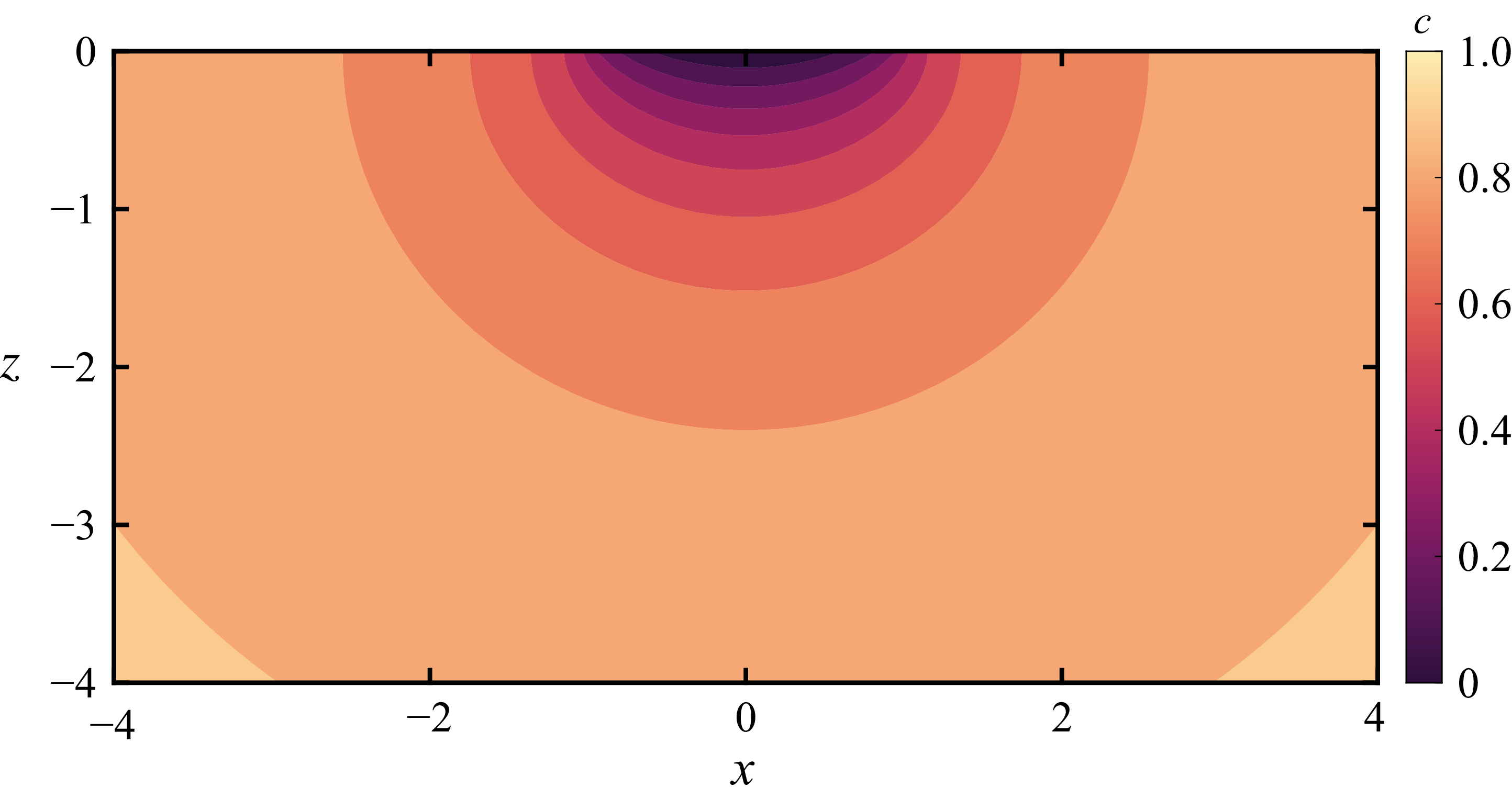

 pg,0≈1.27
 pb,0≈−0.031
 r≈1.1

 Ra=0
 Ra→∞
 κ=0
 z≈−1

 σgm
 Ra=0
 m=0
 σg0=1/2
 O(1)
 R(t)=R0et/2
 m=1
 σg1=0
 O(m1/2)

 σbm
 Ra→∞
 m=0,1
 σb0=σb1=0
 m=2
 O(m1/2)

 m−βRa
 βRa∗m
 m
 limm→∞βRa∗m=96

 Ra=96
 β=1
 Ra

 κ
 κ
 H
 κ∼1−log2|H|
 Ra∗,κ
 m→∞
 H

 M=32
 σbm
 O(M−4)
 σgm


