2.1. Governing equations

The three-dimensional RMI is governed by the multicomponent Navier–Stokes equations in the conservative form (Kawai & Lele Reference Kawai and Lele2008; Tritschler et al. Reference Tritschler, Zubel, Hickel and Adams2014):

(2.1)\begin{gather} \frac{\partial \rho}{\partial t}+\boldsymbol{\nabla}\boldsymbol{\cdot}\left(\rho\boldsymbol{u}\right)=0, \end{gather}

(2.2)\begin{gather} \frac{\partial (\rho\boldsymbol{u})}{\partial t}+\boldsymbol{\nabla}\boldsymbol{\cdot}\left(\rho\boldsymbol{u}\boldsymbol{u}+p{\boldsymbol{\mathsf{I}}}-\boldsymbol{\tau}\right)=0, \end{gather}

(2.3)\begin{gather} \frac{\partial E}{\partial t}+\boldsymbol{\nabla}\boldsymbol{\cdot}\left[E\boldsymbol{u}+\left(p{\boldsymbol{\mathsf{I}}}-\boldsymbol{\tau}\right)\boldsymbol{\cdot}\boldsymbol{u}+\boldsymbol{q}_c+\boldsymbol{q}_d\right]=0, \end{gather}

(2.4)\begin{gather} \frac{\partial (\rho Y_i)}{\partial t}+\boldsymbol{\nabla}\boldsymbol{\cdot}\left(\rho\boldsymbol{u} Y_i\right)-\boldsymbol{\nabla}\boldsymbol{\cdot}\boldsymbol{J}_i=0. \end{gather}

Here, $\rho$ denotes the mixture density, $\boldsymbol {u}=u_x\boldsymbol {i}+u_y\boldsymbol {j}+u_z\boldsymbol {k}$ the velocity, $p$ the pressure and ${\boldsymbol{\mathsf{I}}}$ the identity tensor, where $\boldsymbol {i}$, $\boldsymbol {j}$ and $\boldsymbol {k}$ are unit vectors in the $x$-, $y$- and $z$-directions, respectively. Equations (2.1)–(2.4) are closed with the equation of state for ideal gas

(2.5)\begin{equation} p=\rho\frac{\mathcal{R}}{\bar{M}}T=\left(\bar{\gamma}-1\right)\rho e, \end{equation}

where $\mathcal {R}$ is the ideal gas constant, $\bar {M}$ the molar mass, $T$ the temperature, $\bar {\gamma }$ the ratio of specific heat capacities of the mixture and $e$ the internal energy with

(2.6)\begin{equation} \rho e=E-\tfrac{1}{2}\rho\boldsymbol{u}\boldsymbol{\cdot}\boldsymbol{u}. \end{equation}

In (2.2) and (2.3), the viscous stress tensor

(2.7)\begin{equation} \boldsymbol{\tau}=2\bar{\mu}{\boldsymbol{\mathsf{S}}}-\tfrac{2}{3}\bar{\mu}\left(\boldsymbol{\nabla}\boldsymbol{\cdot}\boldsymbol{u}\right){\boldsymbol{\mathsf{I}}} \end{equation}

for a Newtonian fluid obeys Stokes’ hypothesis (see Graves & Argrow Reference Graves and Argrow1999), where $\bar {\mu }$ is the mixture viscosity, ${\boldsymbol{\mathsf{S}}}=[\boldsymbol {\nabla }\boldsymbol {u}+(\boldsymbol {\nabla }\boldsymbol {u})^{\text {T}}]/2$ the strain-rate tensor and $E$ the total energy per unit volume. In (2.4), $Y_i$ is the mass fraction of species $i$ with $i=1,2$ and $Y_1=1-Y_2$ for two fluids. In (2.3), the heat flux is estimated by Fourier's law

(2.8)\begin{equation} \boldsymbol{q}_c=-\bar{\kappa}\boldsymbol{\nabla} T \end{equation}

with the mixture heat conductivity $\bar {\kappa }$. Moreover, the effect of the enthalpy diffusion flux is incorporated using the interspecies diffusional heat flux (Cook Reference Cook2009)

(2.9)\begin{equation} \boldsymbol{q}_d=\sum_{i=1}^2 h_i\boldsymbol{J}_i \end{equation}

with

(2.10)\begin{equation} \boldsymbol{J}_i = -\rho\left(D_i\boldsymbol{\nabla} Y_i-Y_i\sum_{j=1}^2 D_j\boldsymbol{\nabla} Y_j\right), \end{equation}

where $h_i$ and $D_i$ are, respectively, the enthalpy and the effective binary diffusion coefficient of species $i$. For each species, the viscosity $\mu _i$ is calculated by the Chapman–Enskog model (see Chapman & Cowling Reference Chapman and Cowling1990) and $D_i$ is approximated by the model in Ramshaw (Reference Ramshaw1990). Then the multicomponent/molecular mixing rules are applied to obtain $\bar {M}$, $\bar {\gamma }$, $\bar {\mu }$ and $\bar {\kappa }$ (see Reid, Pransuitz & Poling Reference Reid, Pransuitz and Poling1987). Calculation of these parameters are detailed in appendix A in Tritschler et al. (Reference Tritschler, Zubel, Hickel and Adams2014).

2.2. Initial and boundary conditions

The RMI is simulated in a shock tube in the domain $\varOmega$ within $0\le x,y\le L$ and $-L\le z\le L$. It arises from a weak planar shock wave travelling from a light fluid with $\rho _1$ to a heavy fluid with $\rho _2$ and accelerating the interface between the two fluids. The quantities with subscript 1 or 2 denote those on the light or heavy fluid side, respectively. The single-mode perturbation

(2.11)\begin{equation} \varphi_{I}(\boldsymbol{x})=\frac{z}{a_0}-\cos(kx)\cos(ky)=0 \end{equation}

is imposed on the interface with the amplitude $a_0$, wavenumber $k=2{\rm \pi} /\lambda$ and wavelength $\lambda =L$.

The incident shock, initially at $z=-L/2$, travels along the $z$-direction at the shock Mach number $M_{S}$. The initial preshock state is given by the stagnation pressure $p_0$ and temperature $T_0$ in quiescent fluids, and the density is set to $\rho _i=p_0 M_i/(\mathcal {R}T_0)$ with the species molar mass $M_i$. The post-shock density

(2.12)\begin{equation} \rho_{S}=\frac{\left(\bar{\gamma}+1\right)M_{S}^2}{2+\left(\bar{\gamma}-1\right)M_{S}^2}\rho_1, \end{equation}

pressure

(2.13)\begin{equation} p_{S}=\frac{2\bar{\gamma}M_{S}^2-\bar{\gamma}+1}{\bar{\gamma}+1}p_0 \end{equation}

and velocity $\boldsymbol {U}_{S}=U_{S}\boldsymbol {k}$ with

(2.14)\begin{equation} U_{S}=\frac{2\left(M_{S}^2-1\right)}{\left(\gamma_1+1\right)M_{S}}\sqrt{\frac{\gamma_1 p_0}{\rho_1}} \end{equation}

are calculated by the Rankine–Hugoniot (known as RH) conditions (see Courant & Friedrichs Reference Courant and Friedrichs1999), and the post-shock temperature $T_{S}=p_{S}M_1/(\rho _{S}\mathcal {R})$ is calculated from (2.5).

Initial distributions of the density, pressure, temperature and velocity in the shock tube are sketched in figure 1. They are given by

(2.15)\begin{gather} \rho(\boldsymbol{x},t=0)=\left(\rho_2-\rho_1\right)\mathcal{H}(\varphi_{I})-\left(\rho_{S}-\rho_1\right)\mathcal{H}(z/L+1/2)+\rho_{S}, \end{gather}

(2.16)\begin{gather} \boldsymbol{u}(\boldsymbol{x},t=0)=\left[1-\mathcal{H}(z/L+1/2)\right]U_{S}\boldsymbol{k}, \end{gather}

(2.17)\begin{gather} p(\boldsymbol{x},t=0)=-\left(p_{S}-p_0\right)\mathcal{H}(z/L+1/2)+p_{S}, \end{gather}

(2.18)\begin{gather} T(\boldsymbol{x},t=0)=-\left(T_{S}-T_0\right)\mathcal{H}(z/L+1/2)+T_{S}, \end{gather}

(2.19)\begin{gather} Y_1(\boldsymbol{x},t=0)=1-\mathcal{H}(\varphi_{I}), \end{gather}

where $\mathcal {H}$ denotes the Heaviside function. In the shock tube, periodic boundary conditions are applied in the $x$- and $y$-directions, and the Riemann boundary condition is used in the $z$-direction (see § II.A in Liu & Xiao Reference Liu and Xiao2016).

Figure 1.

Schematic diagram of the initial distribution of the shocked light fluid (SLF), unshocked light fluid (ULF) and unshocked heavy fluid (UHF) with the shock and interface in the shock tube. The symmetry plane in the $x$-direction is colour-coded by $\rho _1\le \rho \le \rho _2$ from blue through white to red.

2.3. DNS

In the present DNS, the density interface is formed by the contact of air (light) and $\textrm {SF}_6$ (heavy). The Atwood number $A=(\rho _2-\rho _1)/(\rho _1+\rho _2)$ for the air–$\textrm {SF}_6$ interface is $A=0.67$ with $M_1=28.964\ \textrm {g}\,\textrm {mol}^{-1}$ and $M_2=146.057\ \textrm {g}\,\textrm {mol}^{-1}$. In order to study the effects of $A$, we artificially vary the molar mass of the heavy fluid, as $M_2=53.7903\ \textrm {g}\,\textrm {mol}^{-1}$ and $260.676\ \textrm {g}\,\textrm {mol}^{-1}$, for additional two DNS cases at $A=0.30$ and $0.80$, respectively.

We set $L=0.1\ \textrm {m}$, $a_0=4\times 10^{-3}\ \textrm {m}$, $p_0=101.3\ \textrm {kPa}$, $T_0=293\ \textrm {K}$ and a low shock Mach number $M_{S}=1.1$ without reshock. To keep the interface in the middle of $\varOmega$ during the evolution, the initial velocity in the $z$-direction is subtracted by $U_0^+$ to offset the interface translation driven by the shock, where $U_0^+$ denotes the post-shock speed of the interface (Yang, Zhang & Sharp Reference Yang, Zhang and Sharp1994) with the superscript ‘+’ for a post-shock quantity.

The DNS for solving (2.1)–(2.4) is carried out by the high-order turbulence solver (HOTS) developed by Liu & Xiao (Reference Liu and Xiao2016). The HOTS is based on the high-order compact difference scheme with localized artificial diffusivity (known as LAD) (see Shankar, Kawai & Lele Reference Shankar, Kawai and Lele2011; Olson & Lele Reference Olson and Lele2013) and parallelized with the message-passing interface. The spatial derivatives in (2.1)–(2.4) and the gradient terms in (2.8) and (2.10), are evaluated using a sixth-order compact finite difference scheme with the artificial diffusivity added near the shock and interface, and the temporal integration is marched by the third-order total-variation-diminishing (known as TVD) Runge–Kutta scheme (Gottlieb & Shu Reference Gottlieb and Shu1998). The HOTS has been validated to be stable and reasonably accurate for DNS of the RMI at $M_{S}\le 1.6$, in which the localized artificial diffusivity does not affect the high accuracy of the numerical results for the interfacial mixing (see Liu & Xiao Reference Liu and Xiao2016; Wu, Liu & Xiao Reference Wu, Liu and Xiao2019).

The computational domain $\varOmega$ is discretized by uniform grid points $N^2\times 2N$ with the mesh spacing $\Delta x=L/N\approx 3.91\times 10^{-4}\ \textrm {m}$ and $N=256$. Two long sponge layers with non-uniform coarse grids are added at $z<-L$ and $z>L$ to avoid the effect of reflected waves at the outlet boundary in the $z$-direction (see Liu & Xiao Reference Liu and Xiao2016). For the finite thickness of the interface and shock, the Heaviside function in (2.15)–(2.19) is approximated by

(2.20)\begin{equation} \mathcal{H}(\alpha) = \frac{1}{2}\left[\mathrm{erf}\left(\frac{\alpha}{2\delta_0}\right)+1\right] \end{equation}

with the initial thickness $\delta _0=4\times 10^{-4}\ \textrm {m}$. The time period for the DNS is from $t=0$ to $t=0.032$ s with the time stepping $\Delta t$ satisfying the Courant–Friedrichs–Lewy condition. Additionally, the initial interface location is shifted to $z=Z_0$ to avoid the long spikes moving out of $\varOmega$. The DNS parameters for the three cases are listed in table 1.

Table 1.

Parameters in three DNS cases.

We conducted a convergence test for the case at $A=0.8$ with $N=64$, 128 and 256. Figure 2 plots the evolution of the scaled amplitude variation $k(a-a_0)$ with the dimensionless time $k\dot {a}_0 t$, and its profiles with various $N$ converge at $N=256$. Furthermore, the baroclinic term in (3.10), which will be investigated in detail, is well-resolved for $N=256$ in our convergence test (not shown). Hence, the resolution $N=256$ is used in the present study.

Figure 2.

Temporal evolution of the scaled amplitude variation in the DNS grid convergence test at $A=0.8$.

Here, the amplitude $a(t)=[a_{s}(t)+a_{b}(t)]/2$ (see Brouillette Reference Brouillette2002) of the interfacial perturbation is the average of the spike amplitude $a_{s}(t)$ and bubble amplitude $a_{b}(t)$. Referencing to the calculation of the mixing width (e.g. Thornber et al. Reference Thornber, Drikakis, Youngs and Williams2010; Oggian et al. Reference Oggian, Drikakis, Youngs and Williams2015), we calculate the spike and bubble amplitudes by integrating the mass fractions as

(2.21)\begin{equation} a_{s}(t)=\int_{-L}^L Y_2(x=0,y=L/2,z,t)\,\mathrm{d} z-L+Z_{I}(t) \end{equation}

and

(2.22)\begin{equation} a_{b}(t)=\int_{-L}^L Y_1(x=0,y=0,z,t)\,\mathrm{d} z-L-Z_{I}(t), \end{equation}

respectively, with $a_{s}(0)=a_{b}(0)=a_0$. Both $a_{s}(t)$ and $a_{b}(t)$ depend on the location of the mean interface plane $Z_{I}(t)$ which is estimated by the interfacial location from the simulation with $a_0=0$ (see Long et al. Reference Long, Krivets, Greenough and Jacobs2009). Then the spike or bubble growth rate $\dot {a}_{s/b}(t)$ is the temporal derivative of $a_{s/b}(t)$, where the subscript ‘$s/b$’ denotes the quantity for spikes $(s)$ or bubbles $(b)$. The initial growth rate $\dot {a}_0=\dot {a}_{s}(0)=\dot {a}_{b}(0)$ is calculated from the initial DNS result at various $A$ and listed in table 1, and $\dot {a}_0$ will be useful in further modelling in § 5. It is noted that, although $\dot {a}_0$ can be approximated using the impulsive model of Richtmyer (Reference Richtmyer1960), the reduction factor in this model can vary significantly with different initial conditions (see Liang et al. Reference Liang, Zhai, Ding and Luo2019).

3.1. Density and pressure distributions as the shock accelerating the interface

When the shock accelerates on the perturbed interface, complex waves are generated, along with significant density and pressure variations in $\varOmega$. Figure 3 sketches three stages of the accelerating process. The shock, located at $z=c(t)$, $-L\le c(t)\le L$, first touches the interfacial trough at $z=-a_0$ and $t=t_{I}$, and then moves away from the interfacial crest at $z=a_0$ and $t=t_{I}+\delta t_{I}$. Assuming that the shock travels at a uniform velocity $S_{I}\boldsymbol {k}$, $S_{I}=M_{S}\sqrt {(\gamma _1p_0)/\rho _1}$ is determined using the Rankine–Hugoniot conditions, and then the accelerating time and period are, respectively, approximated as

(3.1)\begin{equation} t_{I} = \frac{L/2+Z_0-a_0}{S_{I}}=\frac{L+2(Z_0-a_0)}{2M_{S}}\sqrt{\frac{\rho_1}{\gamma_1p_0}} \end{equation}

and

(3.2)\begin{equation} \delta t_{I} = \frac{2a_0}{S_{I}}=\frac{2a_0}{M_{S}}\sqrt{\frac{\rho_1}{\gamma_1p_0}}. \end{equation}

Figure 3.

Schematic diagram for the interaction between the shock and the interface (IF): ($a$) before the incident shock (IS) accelerating the interface; ($b$) during the shock accelerating the interface, when a part of the incident shock becomes the transmitted shock (TS) and reflected shock (RS) is generated; ($c$) after the shock accelerating the interface. Dash lines denote transverse waves behind transmitted and reflected shocks.

Before the incident shock accelerates the interface at $t<t_{I}$ in figure 3($a$), the flow field is divided into a post-shock active region $S$ with a finite velocity driven by the incident shock and two preshock quiescent regions 1 and 2. While the incident shock accelerates the interface at $t_{I}\le t\le t_{I}+\delta t_{I}$ in figure 3($b$), the reflected shock is generated due to $\rho _2>\rho _1$, and the incident shock across the interface becomes a transmitted shock. Due to the compression, the post-shock interface amplitude

(3.3)\begin{equation} a_0^+ \approx a_0-\frac{1}{2}U_0^+\delta t_{I}=\left(1-\frac{U_0^+}{M_{S}}\sqrt{\frac{\rho_1}{\gamma_1p_0}}\right)a_0 \end{equation}

is slightly reduced (see Richtmyer Reference Richtmyer1960), and the interface in (2.11) becomes

(3.4)\begin{equation} \varphi_{I}^+(\boldsymbol{x})=\frac{z}{a_0^+}-\cos(kx)\cos(ky)=0. \end{equation}

Under the interfacial perturbation, both the reflected and transmitted shocks are distorted, followed by transverse waves (see Brouillette Reference Brouillette2002), represented by dashed curves in figure 3(b,c). The transverse waves can further generate more complex waves, e.g. sound waves, and lead to pressure perturbations. In this stage, the flow field is divided into preshock regions 1 and 2 and post-shock regions $S$, 1$^+$ and 2$^+$. The PBV is generated by the shock–interface interaction, which will be discussed in detail in § 3.2. After the transmitted shock leaves the interface at $t>t_{I}+\delta t_{I}$ in figure 3($c$), preshock region 1 disappears. When the transmitted and reflected shocks with transverse waves are remote from the interface, only post-shock regions 1$^+$ and 2$^+$ remain in $\varOmega$.

To obtain the physical quantity $\mathcal {P}$ for $\rho$, $\boldsymbol {u}$, $p$ or $T$ in post-shock regions 1$^+$ and 2$^+$, we decompose

(3.5)\begin{equation} \mathcal{P}(\boldsymbol{x},t)=\mathcal{P}^+(z,t)+\mathcal{P}'(\boldsymbol{x},t) \end{equation}

into a post-shock integral component $\mathcal {P}^+(z,t)$ and a perturbed one $\mathcal {P}'(\boldsymbol {x},t)$. Here $\mathcal {P}^+(z,t)$ is estimated by solving a one-dimensional Riemann problem along the $z$-direction (see Yang et al. Reference Yang, Zhang and Sharp1994). The results indicate that post-shock regions 1$^+$ and 2$^+$ have different $\rho _1^+$ and $\rho _2^+$, and $T_1^+$ and $T_2^+$, whereas have the same $\boldsymbol {U}_0^+=U_0^+\boldsymbol {k}$ and $p_0^+$. The post-shock integral component of the quantities and the post-shock Atwood number

(3.6)\begin{equation} A^+=\frac{\rho_2^+-\rho_1^+}{\rho_1^++\rho_2^+} \end{equation}

in regions 1$^+$ and 2$^+$ in the three DNS cases at various $A$ are calculated and listed in table 2.

Table 2.

Post-shock integral component of the quantities and post-shock Atwood number in the three DNS cases at various $A$.

When the incident shock accelerates the interface at $t_{I}\le t\le t_{I}+\delta t_{I}$, we approximate

(3.7)\begin{gather} \rho^+(\boldsymbol{x},t)=\Delta\rho^+\mathcal{H}(\varphi_{I}^+)+\rho_1^+, \end{gather}

(3.8)\begin{gather} p^+(\boldsymbol{x},t)=-\Delta p^+\mathcal{H}(\xi)+p_0^+ \end{gather}

and

(3.9)\begin{equation} T^+(\boldsymbol{x},t)=\Delta T^+\mathcal{H}(\varphi_{I}^+)+T_1^+, \end{equation}

where the post-shock density and temperature differences across the interface $\varphi _{I}=0$ are $\Delta \rho ^+=\rho _2^+-\rho _1^+$ and $\Delta T^+=T_2^+-T_1^+$, respectively, and the pressure difference across the distorted shock located at $\xi (\boldsymbol {x},t)$=0 is $\Delta p^+=p_0^+-p_0$.

Moreover, $\mathcal {P}'(\boldsymbol {x},t)$ in (3.5) contains effects of the PBV-induced velocity near the interface and of the pressure perturbations from the distorted transmitted/reflected shocks with transverse waves, which will be discussed in § 4.1 in detail.

3.2. Determination of the PBV

Taking the curl of (2.2) yields the vorticity equation

(3.10)\begin{equation} \frac{\textrm{D} \boldsymbol{\omega}}{\textrm{D} t}=\boldsymbol{\omega}\boldsymbol{\cdot}\boldsymbol{\nabla}\boldsymbol{u}-\boldsymbol{\omega}(\boldsymbol{\nabla}\boldsymbol{\cdot}\boldsymbol{u})+\frac{1}{\rho^2}\left(\boldsymbol{\nabla}\rho\times\boldsymbol{\nabla} p\right)+\bar{\nu}\nabla^2\boldsymbol{\omega}, \end{equation}

where $\mathrm {D}/\mathrm {D} t=\partial /\partial t+\boldsymbol {u}\boldsymbol {\cdot }\boldsymbol {\nabla }$ is the material derivative, $\boldsymbol {\omega }=\boldsymbol {\nabla }\times \boldsymbol {u}=\omega _x\boldsymbol {i}+\omega _y\boldsymbol {j}+\omega _z\boldsymbol {k}$ the vorticity and $\bar {\nu }=\bar {\mu }/\rho$ the kinematic mixture viscosity.

We assume that $\boldsymbol {\omega }$ is generated post-shock (see Rasmus et al. Reference Rasmus2018) at the intersection of the shock and interface, and neglect viscous effects (see Samtaney & Zabusky Reference Samtaney and Zabusky1994). Thus only the baroclinic term $(\boldsymbol {\nabla }\rho \times \boldsymbol {\nabla } p)/\rho ^2$ remains on the right-hand side of (3.10). It is noted that the vorticity generation may be very complex from pressure perturbations of distorted shocks and transverse waves (e.g. Samtaney & Zabusky Reference Samtaney and Zabusky1994; Samtaney, Ray & Zabusky Reference Samtaney, Ray and Zabusky1998). As sketched in figure 4, we define that the PBV is generated at the interaction between the interface and the transmitted shock at $\xi (\boldsymbol {x},t)=[z-c(t)]/a_0^+=0$. In other words, we assume that the transmitted shock stays planar by removing the effects of pressure perturbations from distorted waves. Then we calculate the PBV

(3.11)\begin{equation} \boldsymbol{\omega}_{PB}(\boldsymbol{x})=\int_{t_{I}}^{t_{I}+\delta t_{I}}\frac{\textrm{D} \boldsymbol{\omega}}{\textrm{D} t}\,\mathrm{d} t=\int_{t_{I}}^{t_{I}+\delta t_{I}}\dfrac{1}{(\rho^+)^2}\left(\boldsymbol{\nabla}\rho^+\times\boldsymbol{\nabla} p^+\right)\,\mathrm{d} t \end{equation}

by integrating (3.10) between $t_{I}\le t\le t_{I}+\delta t_{I}$ in the Lagrangian view. Starting from (3.7) and (3.8), after some algebra (detailed in appendix A), we derive

(3.12)\begin{equation} \boldsymbol{\omega}_{PB}=\frac{4A^+k\Delta p^+}{\bar{\rho}^+\left(M_{S}\sqrt{\dfrac{\gamma_1 p_0}{\rho_1}}-U_0^+\right)} \delta(\varphi_{I}^+)\left[K_y(x,y)\boldsymbol{i}+K_x(x,y)\boldsymbol{j}\right] \end{equation}

with

(3.13)\begin{equation} K_x(x,y)=\cos(kx)\sin(ky)\ \text{and}\ K_y(x,y)=-\sin(kx)\cos(ky). \end{equation}

Hence, the PBV distribution is symmetric with respect to the interface and the plane $z=0$.

Figure 4.

Schematic diagram of the production of PBV by the misalignment of the pressure gradient across the planar TS with the density gradient across the IF during their interaction.

Without loss of generality, we obtain the initial circulation

(3.14)\begin{equation} \varGamma_0=\iint_{\mathbb{A}}\omega_{{PB},x}(x=0,y,z)\,\mathrm{d} y\,\mathrm{d} z=\frac{(4+2{\rm \pi})A^+a_0\Delta p^+}{M_{S}\bar{\rho}^+}\sqrt{\frac{\rho_1}{\gamma_1 p_0}} \end{equation}

through the right half of the symmetric slice

(3.15)\begin{equation} \mathbb{A}=\left\{(y,z)\,\bigg|\,x=0,\frac{L}{2}\le y\le L,-L\le z\le L\right\} \end{equation}

with $\boldsymbol {\omega }_{{PB}}=\omega _{{PB},x}\boldsymbol {i}$ and $\omega _{{PB},x}>0$ in $\mathbb {A}$. The initial circulations in the present DNS cases are calculated using (3.14) as $\varGamma _0=0.474,0.706$ and 0.617 m$^2$ s$^{-1}$ at $A=0.30,0.67$ and 0.80, respectively.

We remark that $\varGamma _0$ in (3.14) is derived from the PBV in (3.12) rather than approximated by $\dot {a}_0$ in previous vortex models (e.g. Jacobs & Sheeley Reference Jacobs and Sheeley1996; Likhachev & Jacobs Reference Likhachev and Jacobs2005; Morgan et al. Reference Morgan, Aure, Stockero, Greenough, Cabot, Likhachev and Jacobs2012). In addition, a more sophisticated estimation of $\varGamma _0$ was developed in Samtaney & Zabusky (Reference Samtaney and Zabusky1994) and Samtaney et al. (Reference Samtaney, Ray and Zabusky1998) by considering the effects of pressure perturbations such as the three-wave node.

3.3. VSF in the RMI

We use the VSF (see Yang & Pullin Reference Yang and Pullin2010) to visualize the evolution of vortical structures in the RMI. The VSF $\phi _v(\boldsymbol {x},t)$ is a smooth scalar satisfying the constraint $\boldsymbol {\omega }\boldsymbol {\cdot }\boldsymbol {\nabla }\phi _v=0$ so that $\boldsymbol {\omega }$ is tangent at every point (except for vorticity nulls) on an isosurface of $\phi _v$, i.e. each VSF isosurface is a VS consisting of vortex lines. The VSF has been applied to transitional wall flows (Zhao, Yang & Chen Reference Zhao, Yang and Chen2016; Zhao et al. Reference Zhao, Xiong, Yang and Chen2018), fully developed turbulence (Xiong & Yang Reference Xiong and Yang2019b), combustion (Zhou et al. Reference Zhou, You, Xiong, Yang, Thévenin and Chen2019) and magnetohydrodynamics (Hao, Xiong & Yang Reference Hao, Xiong and Yang2019) to characterize vortex dynamics in the Lagrangian view.

Given the PBV in (3.12), the VSF at $t=t_{I}+\delta t_{I}$ is constructed as

(3.16)\begin{equation} \phi_{v0}(\boldsymbol{x})=\frac{z}{a_0^+}-\exp\left({-[\varphi_{I}^+(\boldsymbol{x})]^{2m}}\right)\cos(kx)\cos(ky) \end{equation}

with a weighting index $m$. Appendix B proves that $\phi _{v0}(\boldsymbol {x})=0$ is equivalent to $\varphi _{I}^+(\boldsymbol {x})=0$, so the isosurface of $\phi _{v0}(\boldsymbol {x})=0$ coincides with the interface $\varphi _{I}^+(\boldsymbol {x})=0$ at $t=t_{I}+\delta t_{I}$. We set a large $m=10$ so that $\exp \{-[\varphi _{I}^+(\boldsymbol {x})]^{2m}\}$ decays rapidly for $\varphi _{I}^+\neq 0$. The resultant approximation $\phi _{v0}(\boldsymbol {x})\approx z/a_0^+$ implies that

(3.17)\begin{equation} \phi_{v0}(x,y,-z)\approx-\phi_{v0}(x,y,z) \end{equation}

is antisymmetric in the $z$-direction.

For this single-mode RMI with $\omega _z\approx 0$, we further demonstrate in appendix B that the VSF is simply governed by the Lagrangian transport equation

(3.18)\begin{equation} \frac{\partial \phi_v}{\partial t}+\boldsymbol{u}\boldsymbol{\cdot}\boldsymbol{\nabla}\phi_v=0 \end{equation}

with the initial condition $\phi _v(\boldsymbol {x},t=0)=\phi _{v0}(\boldsymbol {x})$, i.e. the VS $\phi _v(\boldsymbol {x},t)=0$ coincides with the material interface in the entire evolution. The periodic boundary condition is applied for $\phi _v$ in the $x$- and $y$-directions, and an ‘opposite periodic’ boundary condition

(3.19)\begin{equation} \phi_{v0}(x,y,z=L,t)=-\phi_{v0}(x,y,z=-L,t) \end{equation}

is used in the $z$-direction owing to (3.17). The convection term of (3.18) is approximated by the fifth-order weighted essentially non-oscillatory scheme (Jiang & Shu Reference Jiang and Shu1996) and the integration in $t$ is also marched by the third-order total-variation-diminishing Runge–Kutta scheme.

In the numerical implementation, (3.18) is solved along with the DNS. The temporal evolution of the VSF isosurface of $\phi _v=0$ in this RMI at $A=0.67$ is shown in figure 5. The surfaces are colour-coded by $0\le |\boldsymbol {\omega }|/|\boldsymbol {\omega }|_{max}\le 0.8$, where $|\boldsymbol {\omega }|_{max}$ denotes the maximum of $|\boldsymbol {\omega }|$ in $\varOmega$. The moving direction of the surface can be inferred from the vortex lines on the surfaces with the Biot–Savart law. The PBV is deposited on the initial VS at $k\dot {a}_0 (t_{I}+\delta t_{I}) = 0.013$ shortly after the shock accelerating the interface in figure 5($a$), and then evolves through a short linear stage at $k\dot {a}_0 t=1.0$ in figure 5($b$) into asymmetric structures, i.e. spikes (upper part) and bubbles (lower part), in a nonlinear stage at $k\dot {a}_0 t=3.0$ in figure 5($c$). Finally the spikes and bubbles roll up into vortex rings at $k\dot {a}_0 t=10$ in figure 5($d$).

Figure 5.

Temporal evolution of the VSF isosurface of $\phi _v=0$ at ($a$) $k\dot {a}_0(t_{I}+\delta t_{I})=0.013$, ($b$) $k\dot {a}_0 t=1.0$, ($c$) $k\dot {a}_0 t=3.0$ and ($d$) $k\dot {a}_0 t=10$ at $A=0.67$. Some vortex lines are integrated and plotted on the surfaces colour-coded by $0\le |\boldsymbol {\omega }|/|\boldsymbol {\omega }|_{max}\le 0.8$ from blue through white to red.

The VSF isoline of $\phi _v=0$ and contours of $\omega _x$ for various $A$ at a late time $k\dot {a}_0 t=10$ are compared on the slice at $x=0$ in figure 6. We observe that the separation between spikes and bubbles grows with $A$. In general, if the PBV with the same $\varGamma _0$ is added at the initial time, the roll-up of the interface is stronger for smaller $A$ (e.g. Zabusky et al. Reference Zabusky, Kotelnikov, Gulak and Peng2003; Sohn Reference Sohn2004). On the other hand, $\varGamma _0$ calculated by (3.14) in the three DNS cases has the maximum value at $A=0.67$, and $\varGamma _0$ at $A=0.67$ is nearly 1.5 times that at $A=0.30$. As shown in figure 6(b), the vorticity at $A=0.67$ is the most intensive and concentrated within spikes and bubbles, so the case at $A=0.67$ with the notable vortex dynamics is used in the following analysis and modelling.

Figure 6.

Comparison of the VSF isoline of $\phi _v=0$ (solid line) and distribution of $\omega _x$ (colour-coded by $-0.8\le \omega _x/|\omega _x|_{max}\le 0.8$ from blue through white to red) on the slice $x=0$ at $k\dot {a}_0 t=10$ with ($a$) $A=0.30$, ($b$) $A=0.67$ and ($c$) $A=0.80$. The spike and bubble amplitudes calculated by (2.21) and (2.22) at $A=0.67$ are marked in panel ($b$).

4.1. Double-density model of the RMI

As summarized in Nishihara et al. (Reference Nishihara, Wouchuk, Matsuoka, Ishizaki and Zhakhovsky2010), three types of perturbations, the density difference between the perturbed interface, the PBV and the pressure perturbation caused by distorted waves, can trigger the RMI. In order to distinguish the role of each factor, we develop two simplified models, the double-density model (DDM) and the single-density model (SDM).

Initial conditions in the RMI, DDM and SDM are compared in figure 7. In the DDM with the density difference and PBV, the perturbed interface with amplitude $a_0^+$ separates the two fluids. The initial velocity $\boldsymbol {u}_{PB}$ is induced by the PBV in (3.12) for modelling the effect of the incident shock, and the pressure perturbation from distorted waves is excluded. In the SDM only with the PBV, the density is uniform without the interface and incident shock, and the PBV-induced velocity is imposed as in the DDM. Additionally, the VSF is constructed in both models, and the isosurface of $\phi _v=0$ coincides with the interface in the RMI.

Figure 7.

Schematic comparison of the initial conditions of the ($a$) RMI, ($b$) DDM and ($c$) SDM.

In the DDM, the initial flow field at $t=0$ corresponds to that at $t=t_{I}+\delta t_{I}$ after the shock accelerating the interface in the RMI. The initial density, pressure and temperature are modelled by the post-shock integral quantities in regions 1$^+$ and 2$^+$ in figure 3($c$) as

(4.1)\begin{gather} \rho_{DD}(\boldsymbol{x},t=0)=\Delta\rho^+\mathcal{H}(\varphi_{I}^+)+\rho_1^+, \end{gather}

(4.2)\begin{gather} p_{DD}(\boldsymbol{x},t=0)=p_0^+, \end{gather}

(4.3)\begin{gather} T_{DD}(\boldsymbol{x},t=0)=\Delta T^+\mathcal{H}(\varphi_{I}^+)+T_1^+. \end{gather}

The initial velocity

(4.4)\begin{equation} \boldsymbol{u}_{DD}(\boldsymbol{x},t=0)=\boldsymbol{u}_{PB}(\boldsymbol{x}) \end{equation}

is induced by the PBV in (3.12), where

(4.5)\begin{equation} \boldsymbol{u}_{PB}(\boldsymbol{x})=\mathscr{F}^{-1}\left\{\frac{\mathrm{i}\boldsymbol{k}_{F}\times\mathscr{F}\{\boldsymbol{\omega}_{PB}\}}{\left|\boldsymbol{k}_{F}\right|^2}\right\} \end{equation}

is obtained by the Biot–Savart law (see Xiong & Yang Reference Xiong and Yang2019a) with the wavenumber $\boldsymbol {k}_{F}$ in Fourier space and operators of the Fourier transform $\mathscr {F}\{\cdot \}$ and inverse Fourier transform $\mathscr {F}^{-1}\{\cdot \}$. Other fluid quantities $\mu$, $D$, $\gamma$ and $\kappa$ are the same as those in the RMI.

In the SDM, the initial density

(4.6)\begin{equation} \rho_{SD}(\boldsymbol{x},t=0)=\bar{\rho}^+=\tfrac{1}{2}\left(\rho_1^+ +\rho_2^+\right) \end{equation}

and temperature

(4.7)\begin{equation} T_{SD}(\boldsymbol{x},t=0)=\bar{T}^+=\tfrac{1}{2}\left(T_1^+ +T_2^+\right) \end{equation}

are set to the averages of integral ones in post-shock regions 1$^+$ and 2$^+$. The initial pressure and velocity are the same as (4.2) and (4.4) in the DDM, respectively. Then $\mu$, $D$, $\gamma$ and $\kappa$ in the SDM are also set to be the averaged ones.

We examine the DDM and SDM corresponding to the RMI at $A=0.67$. The simulations of the DDM and SDM are essentially the same as the DNS of the RMI except for using different initial conditions and removing the sponge layers. The evolution of the scaled spike and bubble amplitudes $k(a_{s/b}-a_0^+)$ are shown in figure 8, where the dimensionless time for the RMI in figure 8 has $k\dot {a}_0(t_{I}+\delta t_{I})$ subtracted. The amplitudes in the DDM are nearly identical to those in the RMI, and both DDM and RMI show the asymmetric growth of spikes and bubbles. By contrast, the structural evolution is symmetric in the SDM.

Figure 8.

Temporal evolution of the scaled amplitudes of the spike and bubble in the RMI at $A=0.67$ and corresponding DDM, SDM and SDM–SBV (discussed in § 4.4).

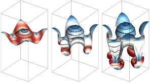
The VSF isosurface of $\phi _v=0$ in the RMI, DDM and SDM are compared at a late time $k\dot {a}_0 t=10$ in figure 9. Note this VS is equivalent to the interface in the RMI and DDM, and there is no interface in the SDM. We observe spikes and bubbles in the RMI and DDM and symmetric structures in the SDM, consistent with the results in figure 8.

Figure 9.

Comparison of the VSF isosurface of $\phi _v=0$ of the ($a$) RMI, ($b$) DDM and ($c$) SDM for $A=0.67$ at $k\dot {a}_0 t=10$. Some vortex lines are integrated and plotted on the vortex surface colour-coded by $0\le |\boldsymbol {\omega }|/|\boldsymbol {\omega }|_{max}\le 0.8$ from blue through white to red.

The nearly identical evolutions in the RMI and DDM demonstrate that the present single-mode RMI is mainly triggered by the density difference across the perturbed interface and PBV, whereas the pressure perturbation from distorted waves can be neglected. Therefore, the dynamical process of the VSF isosurface $\phi _{v0}=0$ driven by the vorticity-induced velocity in the DDM can model the nonlinear growth of the interface in the RMI, and the VS will refer to the isosurface of $\phi _{v0}=0$ in the rest of this paper.

4.2. Generation of the SBV

Next we use the DDM to clarify each role of the density difference and the PBV in the nonlinear evolution of the VS in the RMI. The symmetric slice at $x=0$, containing the essential evolutionary geometry of VSs, is chosen to analyse vortex dynamics in the three-dimensional single-mode RMI. From the symmetries with $u_x=0$, $\omega _y=\omega _z=0$ and $\partial /\partial x=0$, we have simplifications $\boldsymbol {x}=y\boldsymbol {j}+z\boldsymbol {k}$, $\boldsymbol {\nabla }=(\partial /\partial y)\boldsymbol {j}+(\partial /\partial z)\boldsymbol {k}$, $\boldsymbol {u}=u_y\boldsymbol {j}+u_z\boldsymbol {k}$ and $\boldsymbol {\omega }=\omega \boldsymbol {i}$, and presume that the flow is nearly incompressible for low $M_{S}$ without shocks (see Meiron & Meloon Reference Meiron and Meloon1997; Kotelnikov, Ray & Zabusky Reference Kotelnikov, Ray and Zabusky2000). In this way, the vorticity equation (3.10) on the plane $x=0$ is simplified to

(4.8)\begin{equation} \frac{\textrm{D} \omega}{\textrm{D} t} = \frac{1}{\rho^2}\left(\boldsymbol{\nabla}\rho\times\boldsymbol{\nabla} p\right)+\bar{\nu}\nabla^2\omega \end{equation}

with

(4.9)\begin{equation} \boldsymbol{\nabla}\rho\times\boldsymbol{\nabla} p=\frac{\partial \rho}{\partial y}\frac{\partial p}{\partial z}-\frac{\partial \rho}{\partial z}\frac{\partial p}{\partial y}. \end{equation}

Since the viscous term $\bar {\nu }\nabla ^2\omega$ uniformly diffuses $\omega$, the asymmetry of $\omega$ can be only contributed from the baroclinic term $(\boldsymbol {\nabla }\rho \times \boldsymbol {\nabla } p)/\rho ^2$.

The initial density $\rho _0=\rho _{{DD}}$ in (4.1) varies across the interface, so $\boldsymbol {\nabla }\rho _0$ is normal to the VS pointing to the heavy fluid, marked by solid arrows in figure 10($b$). Considering the right half-wave of the VS with the symmetry axis marked by the dash-dotted line in figure 10($b$), $\boldsymbol {\nabla }\rho _0$ is antisymmetric with respect to the symmetry axis.

Figure 10.

Generation mechanism of the SBV. ($a$) Distributions of the initial PBV-induced velocity (vectors) and the pressure perturbation (the contour colour-coded by $-20\ \mathrm {Pa}\le p'_0\le 20\ \mathrm {Pa}$ from blue through white to red) on the slice of $x=0$ within $-L/2\le z\le L/2$. ($b$) Schematic diagram for the generation of the SBV at $t=0^+$ owing to the misalignment of $\boldsymbol {\nabla }\rho _0$ (solid arrows) across the VS with $\boldsymbol {\nabla }\tilde {p}_0$ (open arrows) in the low-pressure region.

Applying the decomposition (3.5) to the initial pressure $\tilde {p}_0$ in the DDM, we have

(4.10)\begin{equation} \tilde{p}_0(\boldsymbol{x})=p_0^+ +p'_0(\boldsymbol{x}). \end{equation}

As the pressure perturbation from distorted waves has been excluded in the DDM, $p'_0(\boldsymbol {x})$ is only generated by the induced velocity of the PBV, and is governed by the variable-density pressure Poisson equation

(4.11)\begin{equation} \nabla^2 p'_0=\frac{1}{\rho_0}\left(\boldsymbol{\nabla}\rho_0\boldsymbol{\cdot}\boldsymbol{\nabla} p'_0\right)-\rho_0\boldsymbol{\nabla}\boldsymbol{u}_{PB}:\boldsymbol{\nabla}\boldsymbol{u}_{PB}, \end{equation}

which is obtained by taking the divergence of (2.2) and neglecting $\boldsymbol {\nabla }\boldsymbol {\cdot }\boldsymbol {u}$. By solving (4.11) using the iteration method with the initial condition $p'_0=0$, $p'_0(\boldsymbol {x})$ is obtained and plotted in figure 10($a$), together with the PBV-induced velocity.

We find that the velocity induced by the PBV is continuous owing to the finite thickness of the interface approximated by (2.20). The distribution of $\boldsymbol {u}_{PB}$ depicts a pair of counter-rotating vortices with the mirror symmetry with respect to the line $x=0, y=L/2$. The vortices produce low pressure regions via (4.11), and $\boldsymbol {\nabla }\tilde {p}_0$ is symmetric with respect to the symmetry axis of the right half of the VS, marked by open arrows in figure 10($b$).

This misalignment of $\boldsymbol {\nabla }\rho _0$ and $\boldsymbol {\nabla }\tilde {p}_0$ produces another type of the baroclinic vorticity, referred to as the SBV. Being different from the PBV, the pressure gradient in the generation of the SBV is due to the low pressure region rather than the discontinuity of the incident shock.

4.3. Spikes and bubbles driven by the SBV

From the Lagrangian view, $\omega$ can be obtained by integrating the right-hand side of (4.8) and decomposed into

(4.12)\begin{equation} \omega(\boldsymbol{x},t)=\omega_{SB}(\boldsymbol{x},t)+\omega_{\nu}(\boldsymbol{x},t)+\omega_0(\boldsymbol{x}) \end{equation}

with the SBV

(4.13)\begin{equation} \omega_{SB}(\boldsymbol{x},t)=\int_0^t\frac{1}{\rho^2(\boldsymbol{x},t')}\left[\boldsymbol{\nabla}\rho(\boldsymbol{x},t')\times\boldsymbol{\nabla} p(\boldsymbol{x},t')\right]\,\mathrm{d} t', \end{equation}

the component produced by the viscous term

(4.14)\begin{equation} \omega_{\nu}(\boldsymbol{x},t)=\int_0^t\bar{\nu}(\boldsymbol{x},t')\nabla^2\omega(\boldsymbol{x},t')\,\mathrm{d} t' \end{equation}

and the initial vorticity $\omega _0 = \omega _{{PB},x}$.

At $t=0^+$ shortly after the initial time in the DDM, the SBV is approximated by $\omega _{{SB}_{0^+}}=(\boldsymbol {\nabla }\rho _0\times \boldsymbol {\nabla }\tilde {p}_0)\Delta t/\rho _0^2$ as sketched by dashed curves with arrows in figure 10($b$). We find that $\omega _{{SB}_{0^+}}$ has opposite signs around the symmetry axis of the right half of the VS.

The synergistic effect of the PBV and SBV on the generation of spikes and bubbles is depicted on the right half of the VS in figure 11($a$). Owing to the opposite signs of $\omega _{{SB}_{0^+}}$, $\omega$ increases and decreases on the two sides of the symmetry axis marked by the dash-dotted line in figure 11($b$), so the vorticity at $t=0^+$ becomes asymmetric. Driven by the induced velocities of the PBV and SBV, the acceleration of the trough and deceleration of the crest of the VS leads to spikes and bubbles in the temporal evolution, respectively, as sketched in figure 11($b$).

Figure 11.

Generation mechanism of spikes and bubbles. ($a$) Contours of $\omega _{{PB}}$ and $\omega _{{SB}_{0^+}}$ at $t=0^+$ on the slice of $x=0$ near the VS. They are colour-coded by $-1.5\times 10^5\ \mathrm {s}^{-1}\le \omega _{PB}\le 1.5\times 10^5\ \mathrm {s}^{-1}$ and $-15\ \mathrm {s}^{-1}\le \omega _{{SB}_{0^+}}\le 15\ \mathrm {s}^{-1}$ from blue through white to red. ($b$) Schematic diagram for the generation of spikes and bubbles (bubb.) owing to acceleration (acc.) and deceleration (dec.) of the VS driven by the SBV.

Therefore, the SBV is not only important in the late mixing stage in the RMI (see Peng et al. Reference Peng, Zabusky and Zhang2003; Zabusky et al. Reference Zabusky, Kotelnikov, Gulak and Peng2003), but also plays a key role in the asymmetric evolution of the VS at early times. To quantify the persistent effects of the SBV, we calculate the evolution of the circulation and its components

(4.15)\begin{equation} \varGamma(t)=\iint_{\mathbb{A}}\omega(\boldsymbol{x},t)\,\mathrm{d} y\,\mathrm{d} z=\gamma_{SB}(t)+\gamma_{\nu}(t)+\varGamma_0 \end{equation}

by integrating (4.12) in region $\mathbb {A}$ in (3.15), where the SBV component $\gamma _{SB}(t)$ and viscous component $\gamma _{\nu }(t)$ are the integrals of $\omega _{SB}(\boldsymbol {x},t)$ and $\omega _{\nu }(\boldsymbol {x},t)$ over $\mathbb {A}$, respectively, and the initial circulation in (3.14) is $\varGamma _0=0.706\ \textrm {m}^{2}\,\textrm {s}^{-1}$ at $A=0.67$. We remark that (4.15) is an approximation, because the dilatation effect is neglected in (4.8).

Moreover, we further divide $\mathbb {A}$ into the spike region $\mathbb {A}_{s}$ and bubble region $\mathbb {A}_{b}$ with $\mathbb {A}=\mathbb {A}_{s}\cup \mathbb {A}_{b}$ based on the evolving vortex surface (see appendix C), and decompose the circulation into

(4.16)\begin{equation} \varGamma(t)=\varGamma_{s}(t)+\varGamma_{b}(t)=\iint_{\mathbb{A}_{s}}\omega(\boldsymbol{x},t)\,\mathrm{d} y\,\mathrm{d} z+\iint_{\mathbb{A}_{b}}\omega(\boldsymbol{x},t)\,\mathrm{d} y\,\mathrm{d} z. \end{equation}

This decomposition also applies to the components in (4.15) as $\gamma _{SB}(t)=\gamma _{SB}^{s}(t)+\gamma _{SB}^{b}(t)$, $\gamma _{\nu }(t)=\gamma _{\nu }^{s}(t)+\gamma _{\nu }^{b}(t)$ and $\varGamma _0=\varGamma _{s}(0)+\varGamma _{b}(0)$ with $\varGamma _{s}(0)=\varGamma _{b}(0)=\varGamma _0/2=0.353\ \textrm {m}^{2}\,\textrm {s}^{-1}$.

The difference in the evolutions of $\varGamma _{s}(t)$ and $\varGamma _{b}(t)$ contributes to the asymmetric growth of the VS via the vorticity-induced velocities (see figure 11). The temporal evolution of circulation variations $\Delta \varGamma _{s/b}=\varGamma _{s/b}-\varGamma _0/2$ and circulation components scaled by $\varGamma _0$ in spike and bubble regions in figure 12 shows that the SBV keeps influencing vortex motions. The positive $\gamma _{SB}^{s}$ in spike regions increases $\omega$ and the negative $\gamma _{SB}^{b}$ in bubble regions decreases $\omega$. Moreover, $\gamma _{SB}^{s/b}$ are very close to $\Delta \varGamma _{s/b}$ in both regions, whereas $\gamma _{\nu }^{s/b}$ can be neglected. Therefore, the nonlinear growth of the interface in the RMI is persistently driven by the SBVs with opposite signs in spike and bubble regions. This SBV effect also provides a physical interpretation for the acceleration/deceleration caused by the perturbation parameter in the perturbation analysis of RMI (see Velikovich et al. Reference Velikovich, Herrmann and Abarzhi2014).

Figure 12.

Temporal evolution of the scaled circulation variations, SBV and viscous components of the circulation in the ($a$) spike and ($b$) bubble regions.

4.4. SDM with the time-varying SBV

The discussions in §§ 4.2 and 4.3 suggest that a major role of the density difference is to produce the SBV which dominates the nonlinear growth of the interface. To further support this important modelling ingredient, we simplify the DDM into the SDM with the time-varying SBV (SDM–SBV). The initial conditions of the SDM–SBV are the same as those in the SDM, including the PBV and uniform density $\bar {\rho }^+$, pressure $p_0^+$ and temperature $\bar {T}^+$, except that a source term is added to the momentum equation (2.2) as

(4.17)\begin{equation} \frac{\partial (\rho\boldsymbol{u})}{\partial t}+\boldsymbol{\nabla}\boldsymbol{\cdot}\left(\rho\boldsymbol{u}\boldsymbol{u}+p{\boldsymbol{\mathsf{I}}}-\boldsymbol{\tau}\right)=\boldsymbol{\varXi}_{SB} \end{equation}

for the simulation of the SDM–SBV. Here, the source term is

(4.18)\begin{equation} \boldsymbol{\varXi}_{SB}=\frac{\partial \left(\rho\boldsymbol{u}_{SB}\right)}{\partial t}, \end{equation}

where the SBV-induced velocity

(4.19)\begin{equation} \boldsymbol{u}_{SB}(\boldsymbol{x})=\mathscr{F}^{-1}\left\{\frac{\mathrm{i}\boldsymbol{k}_{F}\times\mathscr{F}\{\boldsymbol{\omega}_{PB}\}}{\left|\boldsymbol{k}_{F}\right|^2}\right\} \end{equation}

is calculated from the DDM. The evolution of the scaled amplitudes $k(a_{s/b}-a_0^+)$ of the SDM–SBV generally agrees with those in the RMI and DDM in figure 8.

In summary, the nonlinear interfacial evolution of the present RMI can be modelled using the PBV and SBV in a uniform mixture without the density difference and shocks. The PBV first drives the interfacial instability, and then the SBV alters the vorticity distribution, leading to the nonlinear interfacial growth. The evolution of the modelling strategy with the increasing simplification level is illustrated in figure 13.

Figure 13.

Schematic diagram of the simplification from ($a$) the RMI with the IS and IF separating two fluids, through panel ($b$) the DDM with the interface/VS separating two fluids and the imposed PBV, to ($c$) the SDM–SBV with the uniform mixture, imposed the PBV and SBV. The symmetry plane $x=L/2$ is coloured by $\rho _1\le \rho \le \rho _2$ from blue through white to red.

5.1. Vortex-ring model for the RMI

Inspired by the simplifications in the SDM–SBV, we model the interfacial evolution of spikes and bubbles in the RMI by two series of vortex rings moving in opposite directions in a uniform mixture without shocks, so the growth rates $\dot {a}_{s}(t)$ and $\dot {a}_{b}(t)$ are estimated by the velocities of corresponding vortex rings in the $z$-direction. This model in a periodic box is illustrated in figure 14($a$). Considering the periodic boundary conditions, the model with infinite series of vortex rings in the top view is sketched in figure 14($b$).

Figure 14.

Schematic diagram of the vortex-ring model. ($a$) The spike and bubble modelled by vortex rings in a periodic box. The arrows denote the opposite moving directions of vortex rings with rates $\dot {a}_{s}(t)$ and $\dot {a}_{b}(t)$. ($b$) Configuration of periodic vortex rings in the entire domain in the top view. Red and blue rings are, respectively, vortex rings of spikes and bubbles. The arrow denotes vorticity direction and the dash-dotted box the boundary of a periodic box.

The spikes and bubbles are modelled by evolving vortex rings with different circulations. We introduce moving dual polar coordinates to characterize the motion of a vortex ring in figure 15. In this coordinate system moving with the vortex ring, the polar coordinates $(R,\theta )$ are built for the vortex ring with the origin at the ring centre, and $(r,\varphi )$ are built on a cross-section of the ring with the origin at the central axis of the ring. Given the radius $R(t)$ of the vortex ring at a particular time, spatial coordinates $(r,\varphi ,\theta )$, with unit basis $\boldsymbol {e}_r$, $\boldsymbol {e}_{\varphi }$ and $\boldsymbol {e}_{\theta }$, are related to the Cartesian coordinates by

(5.1a,b)\begin{equation} x=\left[R(t)+r\cos\varphi\right]\cos\theta,\quad y=\left[R(t)+r\cos\varphi\right]\sin\theta, \quad z=r\sin\theta. \end{equation}

Figure 15.

Schematic diagram of the moving dual polar coordinates, consisting of ($a$) polar coordinates for the vortex ring and ($b$) polar coordinates on a cross-section of the ring. The red arrow denotes the moving direction of the vortex ring at the rate $\dot {a}_{s}(t)$ or $\dot {a}_{b}(t)$.

We assume that $\boldsymbol {\omega }(\boldsymbol {x},t)=\omega _{\theta }(r,t)\boldsymbol {e}_{\theta }$ is uniform along the $\theta$-direction in this model, then the circulation

(5.2)\begin{equation} \varGamma(t)=\int_0^{2{\rm \pi}}\mathrm{d}\varphi\int_0^{\infty}\omega_{\theta}(r,t)r\,\mathrm{d} r \end{equation}

determines the velocity of the vortex ring. Since figure 12 shows that the circulations vary with time under the influence of the SBV and they are very different between spikes and bubbles, we divide the modelling of $\dot {a}_{s/b}(t)$ into two steps: (i) model the temporal evolution of $\varGamma _{s/b}(t)$ affected by the SBV; (ii) model $\dot {a}_{s/b}(t)$ based on the modelled $\varGamma _{s/b}(t)$ of vortex rings.

5.2. Modelling of circulations based on the SBV

The circulation of vortex rings is estimated by the integration (5.2) of $\omega _{\theta }(r,t)$, which models the SBV effect in the RMI and SDM–SBV. We propose several assumptions on the evolution of vortex rings as follows.

1. (i) All the physical quantities are uniform along the $\theta$-direction, i.e. $\partial /\partial \theta =0$.

2. (ii) The velocity only has the $\varphi$-component and is uniform in the $\varphi$-direction, i.e. $\boldsymbol {u}=u_{\varphi }(r,t)\boldsymbol {e}_{\varphi }$.

3. (iii) The vorticity only has the $\theta$-component and is uniform in the $\theta$-direction, i.e. $\boldsymbol {\omega }=\omega _{\theta }(r,t)\boldsymbol {e}_{\theta }$.

4. (iv) The flow is considered to be incompressible, because it has low $M_{S}$ and no shock (see Meiron & Meloon Reference Meiron and Meloon1997; Kotelnikov et al. Reference Kotelnikov, Ray and Zabusky2000).

Thus the vorticity equation (3.10) is simplified to

(5.3)\begin{equation} \frac{\partial \omega_{\theta}}{\partial t}=\mathcal{B}(\rho,p)+\mathcal{V}(\omega_{\theta}) \end{equation}

with the baroclinic term

(5.4)\begin{equation} \mathcal{B}(\rho,p)=\frac{1}{\rho^2r}\frac{\partial \rho}{\partial \varphi}\frac{\partial p}{\partial r} \end{equation}

and the viscous term

(5.5)\begin{equation} \mathcal{V}(\omega_{\theta})=\bar{\nu}\left(\frac{\partial^2 \omega_{\theta}}{\partial r^2}+\frac{1}{r}\frac{\partial \omega_{\theta}}{\partial r}\right). \end{equation}

Next, we re-express $\mathcal {B}$ and $\mathcal {V}$ in algebraic forms with known quantities.

In the SDM with vanishing $\mathcal {B}(\rho ,p)$, the exact solution of (5.3) (see Tung & Ting Reference Tung and Ting1967; Saffman Reference Saffman1970) is

(5.6a,b)\begin{equation} \omega_{\theta}(r,t)=\frac{\varGamma_0}{4{\rm \pi}\bar{\nu}t}\exp\left({-\frac{r^2}{4\bar{\nu}t}}\right)\quad \text{and}\quad u_{\varphi}(r,t)=\frac{\varGamma_0}{2{\rm \pi} r}\left(1- \exp\left({-\frac{r^2}{4\bar{\nu}t}}\right)\right), \end{equation}

which implies that $\varGamma (t) = \varGamma _0$ is constant.

In the SDM–SBV and RMI, the influence of the SBV is introduced by finite $\mathcal {B}(\rho ,p)$ in (5.3), leading to the time-varying $\varGamma (t)$. From (5.6a,b) and figure 6, we assume that

(5.7)\begin{equation} \omega_{\theta}(r,t)=\frac{\varGamma(t)}{4{\rm \pi}\bar{\nu}t}\exp\left({-\frac{r^2}{4\bar{\nu}t}}\right) \end{equation}

and

(5.8)\begin{equation} u_{\varphi}(r,t)=\frac{\varGamma(t)}{2{\rm \pi} r}\left(1- \exp\left({-\frac{r^2}{4\bar{\nu}t}}\right)\right) \end{equation}

have Gaussian distributions along $r$. From (5.8), the radius of the vortex core

(5.9)\begin{equation} r_{C}(t)=2\sqrt{\bar{\nu}t} \end{equation}

is defined by the distance from the ring centre to the location where $u_{\varphi }$ peaks (see Saffman Reference Saffman1970).

To estimate $\mathcal {B}(\rho ,p)$ in (5.3), we re-express the momentum equation (2.2) as

(5.10)\begin{equation} -\frac{u_{\varphi}^2}{r}=-\frac{1}{\rho}\frac{\partial p}{\partial r} \end{equation}

in cylindrical coordinates with the above assumptions, and then obtain the radial pressure gradient

(5.11)\begin{equation} \frac{\partial p}{\partial r}=\frac{\rho\varGamma^2(t)}{4{\rm \pi}^2r^3}\left(1-\exp\left({-\frac{r^2}{4\bar{\nu}t}}\right)\right)^2. \end{equation}

Subsequently, the azimuthal density gradient in $\mathcal {B}(\rho ,p)$ in (5.4) is produced by the mass transfer owing to the roll-up of the interface between two fluids with $\rho _1^+$ and $\rho _2^+$. Here, $\partial \rho /\partial \varphi$ is positive in the spike region where the heavy fluid is rolled into the light one. On the contrary, it is negative in the bubble region. Thus it is modelled by

(5.12)\begin{equation} \frac{\partial \rho}{\partial \varphi}=\pm\frac{\Delta\rho^+}{\Delta\varphi} \end{equation}

where the upper/lower sign applies to spikes/bubbles, and the variation of the azimuthal angle is calculated by the temporal integral of the angular velocity as

(5.13)\begin{equation} \Delta\varphi=\int_0^t\frac{u_{\varphi}(r,t')}{r}\,\mathrm{d} t'. \end{equation}

To simplify (5.13) by removing the dependence on $r$, we approximate (5.8) by $u_{\varphi }(r,t)=u_{\varphi }(r_{C},t)/2$, roughly the average of $u_{\varphi }$ within the vortex ring. Then we derive

(5.14)\begin{equation} \Delta\varphi=\frac{\left(1-\textrm{e}^{-1}\right)\dot{a}_0}{16{\rm \pi}\bar{\nu}k}\mathcal{G}(\varGamma,t)\quad \text{with}\ \mathcal{G}(\varGamma,t)=\int_0^t\frac{k\varGamma(t')}{\dot{a}_0t'}\,\mathrm{d} t', \end{equation}

where $k$ and $\dot {a}_0$ are introduced to make $\mathcal {G}$ dimensionless. Then (5.12) is approximated by

(5.15)\begin{equation} \frac{\partial \rho}{\partial \varphi}=\frac{\pm 16{\rm \pi}\bar{\nu}k\Delta\rho^+}{\left(1-\textrm{e}^{-1}\right)\dot{a}_0\mathcal{G}(\varGamma,t)}. \end{equation}

Based on the SDM–SBV, we assume the uniform density $\rho =\bar {\rho }^+$ and the uniform averaged mixture kinematic viscosity

(5.16)\begin{equation} \bar{\nu}=\frac{\bar{\mu}}{\bar{\rho}^+}=\frac{\mu_1\sqrt{M_2}+\mu_2\sqrt{M_1}}{\bar{\rho}^+\left(\sqrt{M_1}+\sqrt{M_2}\right)}, \end{equation}

where $\bar {\mu }$ is calculated from Reid et al. (Reference Reid, Pransuitz and Poling1987) and $\mu _1$ and $\mu _2$ are, respectively, determined at $T_1^+$ and $T_2^+$. In the three DNS cases, we obtain $\bar {\nu }=5.61\times 10^{-6},3.74\times 10^{-6}$ and $2.31\times 10^{-6}\ \textrm {m}^{2}\,\textrm {s}^{-1}$ at $A=0.30,0.67$ and 0.80, respectively. Substituting (5.11) and (5.15) into (5.4) and using $A^+ = \Delta \rho ^+/(2\bar {\rho }^+)$ from (3.6) yields

(5.17)\begin{equation} \mathcal{B}=\frac{\pm 8A^+\bar{\nu}k\varGamma^2(t)}{\left(1-\textrm{e}^{-1}\right){\rm \pi}\dot{a}_0r^4\mathcal{G}(\varGamma,t)} \left(1-\exp\left({\frac{r^2}{4\bar{\nu}t}}\right)\right)^2. \end{equation}

Substituting (5.7) into (5.5) yields

(5.18)\begin{equation} \mathcal{V}=\frac{\varGamma(t)}{4{\rm \pi}\bar{\nu}t^2}\left(\frac{r^2}{4\bar{\nu}t}-1\right) \exp\left({-\frac{r^2}{4\bar{\nu}t}}\right). \end{equation}

Substituting (5.17) and (5.18) into (5.3) yields

(5.19)\begin{align} \frac{\partial \omega_{\theta}}{\partial t}&=\frac{\pm 8A^+\bar{\nu}k\varGamma^2(t)}{\left(1- \textrm{e}^{-1}\right){\rm \pi}\dot{a}_0 r^4\mathcal{G}(\varGamma,t)}\left(1-\exp\left({-\frac{r^2}{4\bar{\nu}t}}\right)\right)^2\nonumber\\ &\quad +\frac{\varGamma(t)}{4{\rm \pi}\bar{\nu}t^2}\left(\frac{r^2}{4\bar{\nu}t}-1\right) \exp\left({-\frac{r^2}{4\bar{\nu}t}}\right). \end{align}

Taking the time derivative of (5.7) yields

(5.20)\begin{equation} \frac{\partial \omega_{\theta}}{\partial t}=\frac{1}{4{\rm \pi}\bar{\nu}t}\frac{\textrm{d} \varGamma}{\textrm{d} t} +\frac{\varGamma(t)}{4{\rm \pi}\bar{\nu}t^2}\left(\frac{r^2}{4\bar{\nu}t}-1\right) \exp\left({-\frac{r^2}{4\bar{\nu}t}}\right). \end{equation}

By equating (5.19) and (5.20), we have

(5.21)\begin{equation} \frac{\textrm{d} \varGamma}{\textrm{d} t}=\pm\frac{32A^+k\bar{\nu}^2t\varGamma^2(t)}{\left(1-\textrm{e}^{-1}\right)\dot{a}_0r^4\mathcal{G}(\varGamma,t)} \left(\exp\left({\frac{r^2}{4\bar{\nu}t}}\right)+\exp\left({-\frac{r^2}{4\bar{\nu}t}}\right)-2\right). \end{equation}

This equation is further simplified, in appendix D, by approximating the exponential functions and removing the dependence on $r$.

Finally, we obtain the model equation of circulations for spikes/bubbles

(5.22)\begin{equation} \frac{\textrm{d} \varGamma_{s/b}}{\textrm{d} t}=\frac{\pm 2A^+k\varGamma_{s/b}^2(t)}{\left(1-\textrm{e}^{-1}\right)\dot{a}_0\left(t+t_{\delta}\right)\mathcal{G}(\varGamma_{s/b},t+t_{\delta})} \end{equation}

with the initial condition $\varGamma _{s}(0)=\varGamma _{b}(0)=\varGamma _0/2$. Here, the singularity at $t=0$ in (5.21) is removed by introducing a small $t_{\delta }=\delta _0^2/(4\bar {\nu })$, which is obtained from (5.9) by assuming the initial $r_{C}(t_{\delta })=\delta _0$. Equation (5.22) implies that the SBV dominates the evolution of circulations, consistent with the numerical results in figure 12. We solve (5.22) numerically using the fourth-order Runge–Kutta method, and approximate the numerical solution by

(5.23)\begin{equation} \varGamma_{s/b}(t)=\varGamma_0\left[0.5\pm C_{\varGamma}\left(k\dot{a}_0t\right)^{(({3\pm 1})/{4})A^+}\right] \end{equation}

with constant $C_{\varGamma }=0.15$. In figure 16, the model results in (5.23) and numerical solutions of (5.22) generally agree with DNS results of the RMI, so the explicit expression (5.23) is used in the further modelling. The discrepancies may come from the assumption of $\omega _{\theta }$ in (5.7), e.g. the distribution of $\omega _{\theta }$ at $A=0.30$ or for all the bubbles in figure 6 deviates from the Gaussian one.

Figure 16.

Comparisons of scaled circulations of the ($a$) spike and ($b$) bubble calculated from DNS (symbols), numerical solutions of (5.22) (dashed lines) and the model (5.23) (solid lines) at various $A$.

5.3. Modelling of growth rates using viscous vortex rings

The spike/bubble growth rate is modelled by the velocity of the vortex ring in the $z$-direction in this RMI. This velocity is the superposition of the self-induced velocity of the vortex ring and the induced velocities from infinite other vortex rings due to the periodicity in figure 14($b$). However, the magnitude of the latter part decays as $O(r^{-2})$, so it can be absorbed into the leading terms as an amplification factor $C_0$.

For example, the spike/bubble growth rate at $P_{s}$/$P_{b}$ in figure 14($b$) is approximated by the self-induced velocity of a vortex ring in viscous flows (see Saffman Reference Saffman1970; Fukumoto & Moffatt Reference Fukumoto and Moffatt2008)

(5.24)\begin{equation} \dot{a}_{s/b}(t)=\frac{C_0\varGamma_{s/b}^{E}(t)}{4{\rm \pi}^{4-n}R_{b}(t)} \left[\log \frac{4R_{b}(t)}{\sqrt{\bar{\nu}t}}-3.672\frac{\bar{\nu}t}{R_{b}^2(t)}-0.558\right], \end{equation}

with the number $n=2,3$ of dimensions, where the effective circulation

(5.25)\begin{equation} \varGamma_{s/b}^{E}(t)=\left[1-\exp\left({-\frac{\alpha_{\nu} R_{b}^2(t)}{4\bar{\nu}t}}\right)\right]\varGamma_{s/b}(t) \end{equation}

considers the vorticity cancellation at $r=0$ (see Fukumoto & Kaplanski Reference Fukumoto and Kaplanski2008) with a correction factor $\alpha _{\nu }$ in this RMI. It is noted that although the viscous effect is usually considered to be negligible in the interfacial growth (e.g. Carlès & Popinet Reference Carlès and Popinet2002), it can be notable on the evolution of the vorticity distribution (e.g. Niederhaus & Jacobs Reference Niederhaus and Jacobs2003; Movahed & Johnsen Reference Movahed and Johnsen2013), especially near the vortex core via the vorticity cancellation, so it is still incorporated in (5.24) in our vortex-based modelling.

Then we assume that the spike/bubble radius $R_{s/b}(t)=R_0$ is invariant with time, where the initial radius

(5.26)\begin{equation} R_0=\frac{\displaystyle\iiint_{\varOmega}|\boldsymbol{\omega}_{PB}|\sqrt{x^2+y^2}\,\mathrm{d} V}{\displaystyle\iiint_{\varOmega}|\boldsymbol{\omega}_{PB}|\,\mathrm{d} V}=\frac{1}{k} \end{equation}

is calculated by the weighted-average distance. Since the maximal time scale in this RMI is $O(10^{-2})$ s, $3.672\bar {\nu }t/R_0^2\ll \log (4R_0/\sqrt {\bar {\nu }t})$ is negligible in (5.24). Using a small drift time $t_{\epsilon }$ to remove the temporal singularity at $t=0$, (5.24) becomes

(5.27)\begin{equation} \dot{a}_{s/b}(t)=\frac{C_0}{4{\rm \pi}^{4-n}}k\varGamma_{s/b}(t)\left(1- \exp\left({-\frac{\alpha_{\nu}}{4k^2\bar{\nu}t}}\right)\right) \left[\log\frac{4}{k\sqrt{\bar{\nu}\left(t+t_{\epsilon}\right)}}-0.558\right]. \end{equation}

In the SDM with uniform density and $A=0$, the circulations $\varGamma _{s}(t)=\varGamma _{b}(t)=\varGamma _0/2$ are constant and the growth rates $\dot {a}_{s}(t)=\dot {a}_{b}(t)=\dot {a}_{SD}(t)$ are symmetric. Then we obtain $C_0 = 1.3$ and $\alpha _{\nu } = 1.587\times 10^{-4}$ by fitting $\dot {a}_{SD}(t)$ from the SDM result at $A=0.67$. We remark that the two parameters obtained from this particular case appear to be universal, which is validated by further a posteriori model tests.

Substituting (5.23) and all the parameter values into (5.27), finally we obtain a predictive model for the spike/bubble growth rate as

(5.28)\begin{align} \dot{a}_{s/b}(t)&=\frac{k\varGamma_0}{4{\rm \pi}^{4-n}}\left[0.65\pm 0.195\left(k\dot{a}_0t\right)^{(({3\pm 1})/{4})A^+}\right]\left[1-\exp\left(-\frac{3.97\times 10^{-5}}{k^2\bar{\nu}t}\right)\right]\nonumber\\ &\quad\times\left[\log\frac{4}{k\sqrt{\bar{\nu}\left(t+t_{\epsilon}\right)}}-0.558\right], \end{align}

where the positive/negative sign, respectively, applies to spikes/bubbles, and

(5.29)\begin{equation} t_{\epsilon}=\frac{16}{k^2\bar{\nu}}\exp\left(-12.31{\rm \pi}^{4-n}\frac{\dot{a}_0}{k\varGamma_0}-1.116\right) \end{equation}

is determined from $\dot {a}_{s}(0)=\dot {a}_{b}(0)=\dot {a}_0$. The physical meaning and determination method of the model parameters in (5.28) are summarized in table 3. From (5.28), we find that the nonlinear growth of the RMI mainly depends on $A^+$, and is only slightly mitigated by the viscous effect (see Mikaelian Reference Mikaelian1993; Niederhaus & Jacobs Reference Niederhaus and Jacobs2003; Sohn Reference Sohn2009).

Table 3.

Summary of the parameters in the model (5.28) of growth rates.

5.4. Model assessment

We assess the model in (5.28) using results from the present DNS and other four data sets in the literature, including DNS data of Latini, Schilling & Don (Reference Latini, Schilling and Don2007) and Long et al. (Reference Long, Krivets, Greenough and Jacobs2009) and experimental data of Jacobs & Krivets (Reference Jacobs and Krivets2005) and Liang et al. (Reference Liang, Zhai, Ding and Luo2019) with key parameters summarized in table 4.

Table 4.

Parameters of DNS and experimental series in the literature.

Figure 17 validates the model prediction using the present DNS result of scaled growth rates and amplitude variations at three $A$. In general, our model is able to predict the nonlinear growth of spikes and bubbles, and the predictions (solid lines) agree with the DNS results (symbols) at various $A$. The slight discrepancy of the model prediction is primarily due to the error from the circulation modelling in (5.22) and figure 16. In figure 18, the comparison of the scaled amplitudes from model predictions of (5.28) (solid lines) and various DNS/experimental results (symbols) also shows overall good agreement.

Figure 17.

Comparisons of scaled ($a$) growth rates and ($b$) amplitudes of spikes and bubbles calculated from the DNS results of the RMI (symbols) with the present model (5.28) (solid lines) at various $A$. The growth rates are scaled by $\dot {a}_{0,0.67} \equiv \dot {a}_{0} = 8.50\ \textrm{m s}^{-1}$ at $A=0.67$ for distinguishing results at different $A$.

Figure 18.

Comparisons of scaled spike and bubble amplitudes from the DNS and experimental results (symbols) with the present model (5.28) (solid lines). The line colour corresponds to the symbol colour for the comparison of the same series.

In appendix E, the present model is compared with several existing models of spike and bubble growth rates for all the DNS/experimental series above. In general, the overall prediction from our vortex-based model is comparable or slightly better than the others. Therefore, we demonstrate that the model (5.28) can predict the nonlinear interfacial growth in the RMI at a range of parameters and with various initial conditions.

Compared with existing models, the features of the present one are summarized below.

1. (i) Spike and bubble growth rates are modelled by the motion of vortex rings in viscous flows. The modelling is based on the dynamics of VSs, instead of the asymptotic analysis and empirical matching.

2. (ii) The mechanism of the SBV is elucidated and used to model the increase or decrease of circulations, which leads to enhancement or suppression of the growth of spikes or bubbles, respectively.

3. (iii) The present vortex-based model for two- and three-dimensional RMIs involves time-varying circulations. The initial circulation is derived from the explicit expression of the PBV rather than approximated by the initial growth rate.

On the other hand, the present model is based on the assumption of incompressible flows, so it is restricted to low $M_{S}$, e.g. $M_{S}<1.3$ (see Peng et al. Reference Peng, Zabusky and Zhang2003) in table 4. Additionally, the pressure perturbation by distorted waves and the multimode initial perturbation in the complex RMI with reshocks and turbulent mixing (e.g. Hill, Pantano & Pullin Reference Hill, Pantano and Pullin2006; Pantano et al. Reference Pantano, Deiterding, Hill and Pullin2007) have not been considered.