

1 Introduction
Coastal estuarine ecosystems provide valuable services to society and many are now in decline because of human activities (Barbier et al., Reference Barbier, Hacker, Kennedy, Koch, Stier and Silliman2011). Integrated physical, ecological, and economic modeling can improve understanding of how ecosystem services are affected and the resulting costs and benefits to society. This study relies on such modeling to value water quality improvements in the Chesapeake Bay – the largest estuary in North America and the third largest in the world. The surrounding watershed encompasses 64,000 square miles in parts of six states in the Eastern United States and the District of Columbia, and is home to about 18 million people. The Chesapeake Bay’s unique set of ecological and cultural elements has motivated efforts to preserve and restore its condition for more than 25 years; however excess nutrient and sediment pollution continues to degrade water quality and adversely affect the provision of ecosystem services. In December 2010 a pollution budget that puts limits on nutrient and sediment inflows from the surrounding watershed, called a Total Maximum Daily Load (TMDL), was established for compliance with the Clean Water Act. The Chesapeake Bay TMDL requires loadings of nitrogen, phosphorus, and sediment to be reduced by 25%, 24%, and 20%, respectively, by the year 2025.Footnote 2
Those who live near or visit the Chesapeake Bay will benefit from improved water clarity, enhanced recreational experiences, and better conditions for aquatic wildlife. Achieving these improvements in the Bay requires management practices throughout the watershed that also improve water quality in freshwater lakes (Moore et al., Reference Moore, Johnston, Smith and Milstead2011). Van Houtven et al. (Reference Van Houtven, Mansfield, Phaneuf, von Haefen, Milstead, Kenny and Reckhow2014) estimate the economic benefits from such improvements to lakes in the part of the watershed that lies within Virginia. In this paper we estimate benefits from improvements to lakes throughout the entire watershed and to the Chesapeake Bay itself. The design of our study also allows us to isolate the willingness to pay (WTP) for freshwater improvements from those in the Bay and perform a comparison between the two categories of benefits. In addition to ancillary benefits from freshwater lakes, estimating the total economic value of the expected improvements requires capturing nonuse value as well. Nonuse value accrues to people who may never visit these waterbodies but benefit from the improvements because of a sense of stewardship, a desire to preserve the resource for future generations, or other reasons. While benefits to users of aquatic resources can be measured using revealed preference approaches, only stated preference (SP) methods can capture nonuse values, which may be substantial for an iconic estuary like the Chesapeake Bay.
Cropper and Isaac (Reference Cropper and Isaac2011) review valuation studies relevant to improving water quality in the Chesapeake Bay and find very few estimates of total or nonuse benefits of improved water quality. Bockstael, McConnell and Strand (Reference Bockstael, McConnell and Strand1988, Reference Bockstael, McConnell and Strand1989) estimate WTP to make the Bay ‘swimmable’ for those respondents who considered it unacceptable for swimming. Lipton (Reference Lipton2004) estimates WTP of nonusers for restoring oyster reefs in the Chesapeake Bay using a broad, but nonrandom, sample that covered most Mid-Atlantic States. Hicks et al. (Reference Hicks, Kirkley, McConnell, Ryan, Scott and Strand2008) examine a broader variety of environmental outcomes associated with reduced sediment and nutrient loads in the Bay, but cost is not included as an attribute in their survey, and so WTP cannot be inferred. Together, these studies provide limited information about values for new clean-up programs in the Chesapeake Bay.
Transferring estimates from studies of related resources could provide an alternative method for valuing the Bay, but this information is also limited. Although Johnston et al. (Reference Johnston, Grigalunas, Opaluch, Mazzotta and Diamantedes2002) estimate the benefits of resource preservation and restoration in the Peconic Estuary, another estuary in the Eastern United States, the attributes used to value the improvements (acres of farmland, undeveloped land, wetlands, shellfishing areas, and aquatic grasses) have limited applicability to the Bay. Transferring benefits for improvements to lakes is more feasible because of the number of candidate studies available in the literature (e.g. Roberts Boyer & Lusk, Reference Roberts, Boyer and Lusk2008; Viscusi, Huber & Bell, Reference Viscusi, Huber and Bell2008; Herriges et al., Reference Herriges, Kling, Liu and Tobias2010; Phaneuf et al., Reference Phaneuf, von Haefen, Mansfield and Van Houtven2013; Van Houtven et al., Reference Van Houtven, Mansfield, Phaneuf, von Haefen, Milstead, Kenny and Reckhow2014). While these studies provide values that may be applicable to freshwater improvements in the Chesapeake Bay Watershed, it would not be appropriate to estimate a WTP value for the Bay separately and combine them for a number or reasons, including substitutability between watershed lakes and the Bay.
To estimate the total economic value of the benefits expected as a result of the Chesapeake Bay TMDL, we conduct an SP survey of residents living in 17 Eastern states and the District of Columbia. The survey employed a discrete choice experiment (DCE) response format to estimate WTP for improvements in five environmental attributes: water clarity; populations of three Chesapeake species (striped bass, blue crab, and Eastern oysters); and the condition of freshwater lakes in the Chesapeake Bay Watershed. The DCE response format allows us to estimate marginal WTP for each attribute, as well as total WTP for outcomes expected from the TMDL. We rely on a combination of integrated hydrological and ecological modeling and expert judgment to obtain projections of the effects of the TMDL on the environmental attributes.
Our study fills a key gap in the literature by simultaneously valuing water quality outcomes for the Chesapeake Bay itself and freshwater lakes in the watershed. Such an approach is essential to evaluate the benefits of policies such as the TMDL, which have the potential to affect thousands of water bodies. The environmental improvements projected to result from the TMDL yield estimated benefits of $3.9 billion to $6.8 billion per year. Great care is taken to minimize potential biases, both in the survey design and econometric analysis stages of this research. We are also able to obtain distinct values for water quality improvements for both users and nonusers of the resources, using information obtained from a follow-up questionnaire administered to households who did not respond to the main survey.
2 Survey design
The survey instrument was designed through extensive focus groups held in several locations, both within and outside of the Chesapeake Bay Watershed.Footnote 3 The foremost goals of the focus groups were (1) to identify the environmental attributes that were the most salient to respondents and that would be affected by the TMDL, and (2) to develop an information section that educates the respondent without influencing their responses and remains brief enough to prevent fatigue. We limited the attributes used to describe the policy outcomes to those that are likely to enter household utility functions directly, rather than inputs into an ecological production function (Boyd & Krupnick, Reference Boyd and Krupnick2009, Reference Boyd and Krupnick2013).
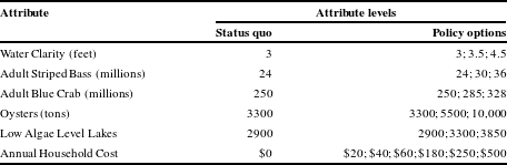
The chosen attributes and attribute levels are shown in Table 1, including costs, which were presented as an increase in a household’s annual cost of living. The payment vehicle was chosen because it was germane to focus group participants inside and outside of the watershed. More typical payment vehicles such as an increase in taxes or utility bills are only feasible for households in states directly affected by the TMDL. The information treatment included a description of how costs imposed on industry within the watershed would increase prices of goods sold elsewhere, thus increasing the cost of living for households outside the watershed. The metrics describing each of the environmental attributes were chosen based on what focus group participants found to be most tangible (e.g., feet of water clarity, number of striped bass, number of crabs). To provide points of reference to which respondents could relate these levels to personal experiences, the survey briefly described the levels of each attribute historically, and within the last 20 years. Focus group participants stated that these reference levels were more salient than references to “pristine” conditions or policy goals. The attribute levels were chosen to ensure appropriate coverage for potential policy applications, and were informed by consultation with the EPA’s Chesapeake Bay Program Office and preliminary water quality and ecological model projections (see Section 5).
Attributes and attribute levels.

In order to achieve the nutrient pollution reductions required by the TMDL, management practices are required throughout the Chesapeake Bay Watershed to prevent excess nitrogen and phosphorus from entering rivers and streams that eventually reach the Bay. Many of these rivers and streams also feed into lakes and reservoirs. Therefore, reducing nutrients in the Bay also reduces these pollutants in over 4200 freshwater lakes in the watershed. To capture this additional benefit, we describe conditions in hyper-trophic lakes and lakes with lower trophic classifications for respondents in terms of appearance, odor, and the types of fish that would be most prevalent. The attribute “Low Algae Level Lakes” was chosen to express this ecological change with a unidimensional numerical metric – the number of lakes with “low algae levels” – which marks ecological improvements with increases in the measure. The information treatment described lakes with low algae as having clear blue or brown water, with three to six feet of visibility, and favoring game fish like bass and trout. High algae lakes were described as having green water with 2 feet of visibility or less, conditions favoring rough fish species like catfish and carp, and having an unpleasant odor on warm days.
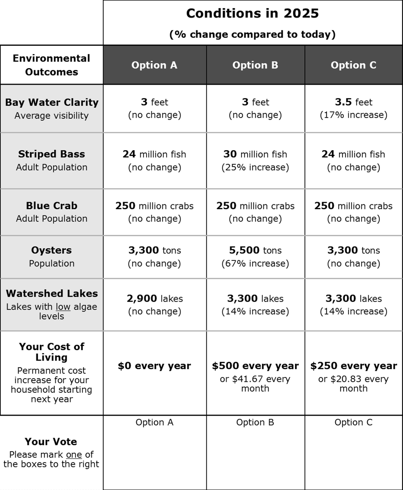
Example of choice question.

The survey includes three choice questions. As shown in the example in Figure 1, each question presents a status quo option with baseline attribute levels and zero cost, and two policy options with some or all of the attributes improving and positive costs. Baseline and policy attribute levels represent conditions in the year 2025 because management practices will be implemented over time and most require additional time to generate ecological or aesthetic improvements. The attribute levels are presented in both absolute terms and relative to current conditions. Respondents are asked to choose one of the three options in each choice question. Alternative levels are based on an orthogonal fractional factorial design; alternative pairs reflect tradeoffs at the margin (i.e., improvements in the attributes that are attained at the cost of decreases in other environmental attributes and/or increase in the cost of the “policy”). Finally, these pairs are grouped to maximize the variability of the environmental and cost attributes within and across individual surveys.
3 Data
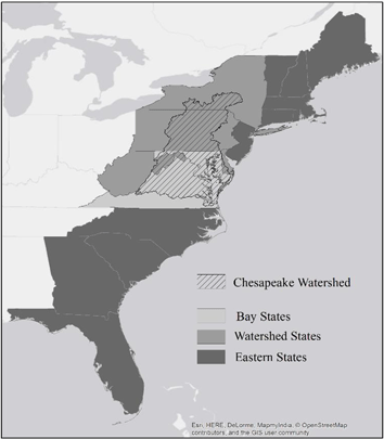
The survey was administered via mail to a random sample of individuals 18 years of age or older who reside in the District of Columbia or one of 17 U.S. states that contain at least part of the Chesapeake Bay Watershed or lie within 100 miles of the Eastern coast of the United States. The sample was stratified by geographic region based on proximity to the Chesapeake Bay and the surrounding watershed, as shown in Figure 2.
Sample area and geographic strata.

The sample was allocated in equal proportions of one-third for each stratum, thus leading to the highest sampling rate in the Bay States stratum (which has the lowest population, about 5.4 million households), and the lowest sampling rate in the Other Eastern States stratum (which has the highest population, about 25.4 million households). The survey was administered to 2829 households, 943 in each geographic stratum. After accounting for ineligible addresses, the response rate varied across the strata: 34% in the Bay States, 30% in the Watershed States, and 27% in the Other Eastern States.
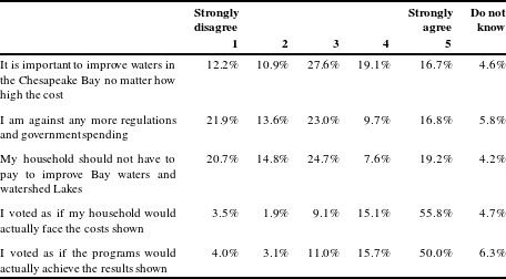
The survey included several questions to probe the respondents’ familiarity and experience with the Chesapeake Bay and freshwater lakes in the watershed. Most of the sample had heard of the Chesapeake Bay (94%) and knew that excess nutrients and sediment could degrade water quality (80%). About a third of the sample reported visiting the Bay (35%) or lakes in the watershed (32%) in the last 5 years for recreational purposes. Table 2 summarizes the responses to debriefing questions that probe the respondents’ attitudes related to environmental regulation as well as their comprehension of the choice task and background information. When asked if “It is important to improve waters in the Chesapeake Bay no matter how high the cost,” 38% of the respondents agreed or strongly agreed. About 27% of respondents indicated they were against more regulations and government spending and about the same amount felt they should not have to pay to improve water quality in the Chesapeake Bay.
Responses to attitudinal debriefing questions. a

a Unweighted sample statistics based on full sample of
 $n=671$
respondents (unscreened). Percentages do not necessarily sum to 100% due to some respondents skipping individual questions.
In addition to design choices to minimize biases (e.g., reminders about budget constraints), we use a multi-faceted approach to screen for respondents who exhibit several sources of potential bias, including protest responses, scenario rejection, and hypothetical bias. Specifically, we used the choice questions and debriefing questions to identify and remove respondents who exhibited evidence of these behaviors as follows:
Protest - Respondent always chose status quo in the choice questions, and agreed or strongly agreed with the statements “I am against any more regulations and government spending” and “My household should not have to pay any amount to improve Bay Waters and Watershed lakes.”
Warm glow – Respondent always chose most expensive option in the choice questions, and agreed or strongly agreed with the statement “It is important to improve waters in the Chesapeake Bay Watershed, no matter how high the costs.”
Hypothetical bias – Respondent always chose a policy option in the choice questions, and disagreed or strongly disagreed with the statement “I voted as if my household would actually face the costs shown in the questions.”
Scenario Rejection – Respondents who disagreed or strongly disagreed with the statement “I voted as if the programs would actually achieve the results shown by 2025.”
Table 3 displays the number of respondents identified under each of the screening criteria. The original unscreened sample includes 671 respondents who answered at least one of the choice questions. The main regression results and WTP estimates are based on the 559 respondents who were not eliminated for protest, warm glow, scenario rejection, or hypothetical bias (see rightmost column in Table 3). Responses were weighted to account for different sampling intensities, response rates, and screening results to ensure that sampled households appropriately represent the population across the geographic strata.
Number of respondents under alternative screening criteria. a

a Categories are not mutually exclusive. A respondent can exhibit more than one type of bias.
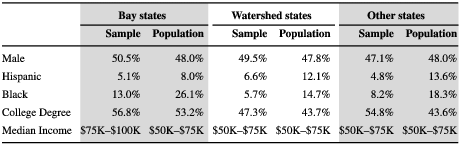
Table 4 presents the characteristics of the final sample of respondents (
 $n=559$
) compared to the total population within each stratum. The sample is representative in terms of the proportion of respondents that are male, but does contain fewer minorities than the corresponding population. The sample also contains a higher proportion of people with at least a 4-year college degree compared to the population, though this difference is only significant in the Other Eastern States strata. The median income category of the sample matches that of the population in the Watershed and Other Eastern States but is higher in the Bay States stratum.Footnote
4
Sample and population demographic comparisons.

In order to determine if and how respondents and nonrespondents differ in ways that we cannot observe using census data, we conducted a nonresponse study (NRS) in which a short questionnaire was administered to a random sample of households that received the main survey but did not complete and return it. The NRS questionnaire included awareness, attitudinal, and demographic questions to examine differences between respondents and nonrespondents. We included an unconditional $2 cash incentive to encourage participation. The NRS received a 19% response rate, yielding 263 completed NRS surveys.
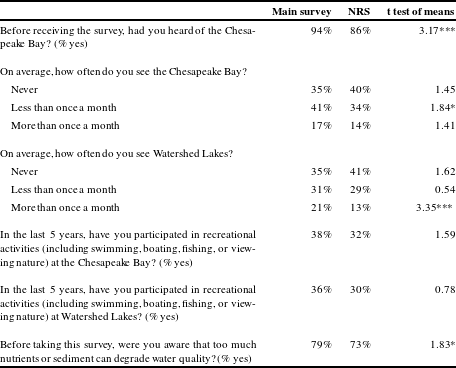
After a brief introduction, the NRS questionnaire poses four questions about individuals’ awareness and use of the Chesapeake Bay and Watershed lakes. Familiarity and use of the Bay may be correlated with WTP for improvements (Johnston et al., Reference Johnston, Opaluch, Magnusson and Mazzotta2005) and therefore it is important to assess whether there are systematic differences between respondents and nonrespondents. Table 5 compares the percentage of positive responses to these questions. In general, respondents to the main survey have similar levels of familiarity with the Bay compared to nonrespondents (i.e., those who completed the NRS questionnaire). Main survey respondents are more likely to have heard of the Bay, viewed the Bay and lakes more frequently, and are slightly more familiar with pollution issues in the Bay compared to the nonrespondents.
Comparison of familiarity with the Chesapeake bay watershed and watershed issues.

***
 $p<0.01$
, **
 $p<0.05$
, *
 $p<0.1$
.
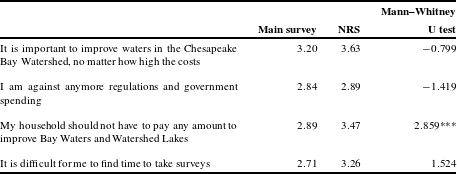
We also examine attitudes toward regulation and environmental issues in respondents versus nonrespondents, which could affect the likelihood of participating in the survey and WTP. Table 6 shows the mean response to each question (on a scale of
 $1=$
Strongly Disagree to
 $5=$
Strongly Agree) and the results of Mann–Whitney tests comparing the distributions of responses across samples. Again, the main survey respondents and NRS respondents are very similar, with the exception that nonrespondents are more likely to believe households should not have to pay for water quality improvements.
Comparison of attitudinal responses.

***
 $p<0.01$
, **
 $p<0.05$
, *
 $p<0.1$
.
Data from the main survey and the NRS suggest there is some potential for nonresponse bias.Footnote 5 People who are familiar with the Chesapeake Bay and were aware of nutrient and sediment pollution before receiving the main survey were more likely to complete and return it than the NRS sample. While only a few of these differences are statistically significant, respondents’ experiences could influence their responses to the policy choice questions and our WTP estimates. Data from the attitudinal questions, however, are less conclusive. The two samples have very similar attitudes toward more regulation and government spending. NRS respondents are just as likely to agree that water quality should be improved regardless of cost but are also more likely to say that their household should not have to pay for those improvements.
4 Statistical model
In the random utility model, utility is composed of a deterministic component,
 $v(\cdot )$
, and an unobserved random component
 $\unicode[STIX]{x1D700}$
. The utility
 $u_{ij}$
experienced by household
 $i$
from alternative
 $j$
is defined by the conditional indirect utility function:
 $$\begin{eqnarray}u_{ij}=v(\boldsymbol{x}_{\boldsymbol{j}},Y_{i}-C_{j})+\unicode[STIX]{x1D700}_{ij}=v_{ij}+\unicode[STIX]{x1D700}_{ij}.\end{eqnarray}$$
The deterministic component is a function of a vector of attributes describing the alternative
 $\boldsymbol{x}_{\boldsymbol{j}}$
, as well as numeraire consumption,
 $Y_{i}-C_{j}$
(household income minus the cost of alternative
 $j$
). When
 $\unicode[STIX]{x1D700}$
is assumed to be independently and identically distributed as type I extreme value, the model can be estimated as a conditional or mixed logit (Maddala, Reference Maddala1983; Greene, Reference Greene2003; Train, Reference Train2009).
In addition to attributes of the choice alternatives we include an indicator variable identifying the status quo alternative, allowing us to estimate a status quo constant (SQC). A positive and statistically significant SQC indicates a tendency to favor the status quo that is not explained by the attributes or other variables in the estimating equation. A negative and significant SQC indicates the opposite tendency – a preference for the policy options. To allow for both possibilities, we estimate a random parameters logit and allow the SQC to vary across respondents; other coefficients are treated as fixed parameters.Footnote 6
The literature offers no clear guidance regarding the choice of specific functional forms for
 $v(\cdot )$
when analyzing choice experiment data. In practice, researchers often use linear forms (Johnston et al., Reference Johnston, Swallow, Tyrrell and Bauer2003), although some have applied more flexible forms to allow for nonlinearities over the attribute space (Cummings, Ganderton & McGuckin, Reference Cummings, Ganderton and McGuckin1994). We adopt a linear model and log-transform the environmental attributes in order to capture diminishing marginal utility while preserving more degrees of freedom than a model with higher order effects. Using this specification of
 $v(\cdot )$
, the conditional probability that household
 $i$
would choose alternative
 $j$
is
 $$\begin{eqnarray}P_{i}(j|x_{k},C_{k})=\frac{\exp (SQC_{i}\cdot d_{j}+\unicode[STIX]{x1D6FD}\ln (x_{j})+\unicode[STIX]{x1D6FE}C_{j})}{\mathop{\sum }_{k}\exp (SQC_{i}\cdot d_{k}+\unicode[STIX]{x1D6FD}\ln (x_{k})+\unicode[STIX]{x1D6FE}C_{k})},\end{eqnarray}$$
where
 $k$
indexes the alternatives,
 $d$
is a dummy variable indicating the status quo alternatives,
 $\unicode[STIX]{x1D6FD}$
is a vector of coefficients on the choice attributes, and
 $\unicode[STIX]{x1D6FE}$
is the negative of the marginal utility of income. The
 $i$
subscript on SQC appears because that estimated coefficient is allowed to vary across respondents whereas
 $\unicode[STIX]{x1D6FD}$
and
 $\unicode[STIX]{x1D6FE}$
are not. We also expand the model to test the effect of user status on the choice probabilities by interacting dummy variables for Bay and lake users with the corresponding choice attributes.
The survey included questions to probe the effect of possible omitted variables on the respondents’ choices. Specifically, we wanted to learn whether respondents considered improvements to lakes outside of the watershed, which in reality would not be affected by the Chesapeake Bay TMDL, or changes in the price and quality of seafood, which are market impacts that we want to exclude from the estimation of the nonmarket benefits. Some evidence of these potentially confounding considerations was found during focus group testing and cognitive interviews. Survey respondents were told not to consider these additional impacts, however approximately half of the sample (50.3%) indicated that improvements to lakes outside of the watershed affected their choice. About a third of respondents (36%) said changes in seafood price and quality had an impact on their choice. To test and control for potential omitted variable bias, in some models we interact indicator variables identifying those respondents with the associated attributes.
5 Results
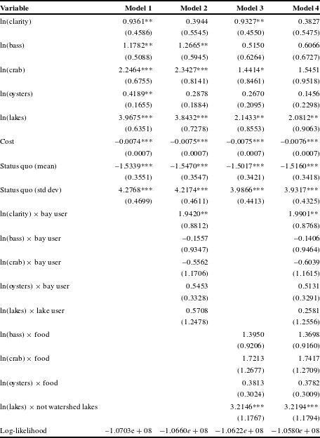
The mixed logit model is estimated via maximum simulated likelihood using 1000 Halton draws (Train, Reference Train2009). Since each respondent faces three choice tasks, we account for the panel structure of the data with standard errors clustered at the respondent level. Table 7 presents the results of four different models. Model 1 is the most parsimonious specification including only the status quo dummy variable, the natural log of the environmental attribute levels, and cost. Model 2 adds interactions between user status and attributes. Models 3 and 4 add the omitted variable interactions to the first two specifications.
Mixed logit regression results.

***
 $p<0.01$
, **
 $p<0.05$
, *
 $p<0.1$
. Standard errors in parentheses, clustered at the respondent level. Mixed logit models estimated using 1000 Halton draws, using on
 $n=4719$
observations (559 respondents).
The estimated coefficients on all attributes and the cost variable are statistically significant with the expected sign in Model 1. The SQC has a negative and statistically significant mean indicating an average tendency to favor the policy options over the status quo that is not explained by the other variables. The standard deviation on the SQC is also statistically significant, indicating strong heterogeneity in this tendency and justifying the decision to estimate a random coefficient for the status quo variable.
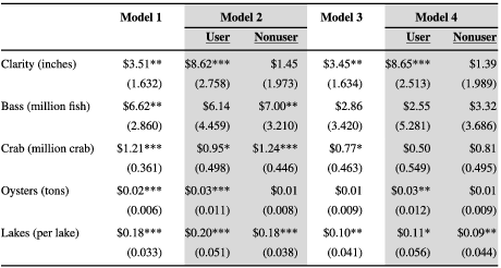
In Model 2 we add interaction terms between the Bay attributes (clarity, bass, crab, and oysters) and a dummy variable for active users of the Bay, as well as an interaction term between the watershed lakes attribute and a dummy variable identifying users of watershed lakes. Active users are defined as those who participated in recreational activities (e.g., swimming, boating, fishing, or viewing nature) at the Chesapeake Bay (for bay users) or watershed lakes (for lake users) within the last 5 years. Coefficient estimates on most attributes are similar to Model 1, indicating that those attributes have a similar impact on choices for users and nonusers. The notable exception is Bay water clarity. The coefficient on the uninteracted clarity variable is no longer significant but the coefficient on the user-interacted clarity variable is significant and large. This indicates that water clarity is important to users of the Bay, and that they are willing to pay significantly more than nonusers for improvements.
Models 3 and 4 add interaction terms to test and control for the effect of respondents’ potential consideration of additional impacts on the results. The interaction terms between bass, crab, and oysters with food are insignificant in both models, suggesting that consideration of seafood price or quality did not lead to systematically different responses. In contrast, the coefficients on ln(lakes)
 $\times$
not watershed lakes are positive and significant, suggesting that respondents who said they were considering lakes outside the watershed when answering the choice questions are willing to pay more for lake improvements than the rest of the sample. To examine the effects that user status and consideration of omitted variables have on the estimated benefits we next calculate WTP.
Given our specification of the utility function, at some reference level
 $\breve{x}_{k}$
the marginal willingness to pay (MWTP) for attribute
 $x_{k}$
is:
 $$\begin{eqnarray}\frac{\unicode[STIX]{x2202}u/\unicode[STIX]{x2202}x_{k}}{-\unicode[STIX]{x2202}u/\unicode[STIX]{x2202}C}=\frac{\unicode[STIX]{x1D6FD}}{-\unicode[STIX]{x1D6FE}\breve{x}_{k}}.\end{eqnarray}$$
The MWTP values presented below use the status quo attribute levels for
 $\breve{x}_{k}$
. When calculating MWTP, as well as the household and total WTP values presented later, we remove the SQC and omitted variable interactions from the calculations, thereby controlling for potential status quo and omitted variable biases. Looking first at Model 1 (Table 8), we see that the MWTP estimates are positive and significant for all attributes. Estimated annual WTP for a one-inch increase in Bay water clarity is $3.51. Respondents are willing to pay $6.62 per year to increase the population of striped bass by one million, $1.21 for one million additional blue crabs, and about $0.02 for a one-ton increase in oysters. Finally, moving one hyper-eutrophic lake to a lower trophic category is valued at $0.18 per respondent per year.
Marginal willingness to pay estimates (2014 dollars).

***
 $p<0.01$
, **
 $p<0.05$
, *
 $p<0.1$
. Bootstrapped standard errors in parentheses (1000 bootstrap iterations).
Model 2 allows for the comparison of MWTP between users and nonusers. Users of the Bay hold a significantly higher MWTP of $8.62 per year for a one-inch improvement in clarity, compared to nonusers for whom MWTP is not significant. The MWTP values between users and nonusers are fairly similar for crabs and lakes. The point estimates are also similar for bass and oysters, although the former is statistically significant only among nonusers and the latter among users.Footnote 7
Models 3 and 4 included interaction terms to account for WTP differentials among respondents who stated that they considered variables omitted from our choice experiment – the price or quality of seafood and lakes outside the watershed. The corresponding coefficients were not included in the MWTP calculations, and so these potential sources of bias are controlled for. Models 3 and 4 yield similar MWTP estimates for bay water clarity as Models 1 and 2, suggesting that MWTP for clarity is stable after controlling for omitted variable bias. The MWTP for increases in fish and shellfish populations, on the other hand, are noticeably lower and are often no longer statistically significant; this suggests that respondents considering the price and quality of seafood have a higher WTP for improvements in fish populations. Similarly, by omitting any premium held by respondents who considered improvements to lakes outside the watershed, the MWTP for lakes is reduced by about half, but remains statistically significant.
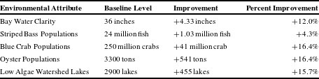
Next we estimate household WTP for projected improvements as a result of the TMDL. The projected changes for the attributes included in the choice questions are presented in Table 9. Improvements in water clarity from the TMDL were provided by the EPA Chesapeake Bay Program Office. The Chesapeake Bay Estuary Model projects spatially explicit water clarity levels across the Bay and tidal tributaries under baseline and TMDL conditions.Footnote
8
 $^{,}$
Footnote
9
According to the Estuary Model, the largest gains in water clarity are expected in the upper Bay and tidal tributaries, with smaller improvements occurring closer to the mouth of the Bay. We use an average improvement across the Bay and tidal tributaries in our calculations.
The changes in striped bass, blue crab, and oyster populations are based on a summary of expert judgments from a panel of six water quality and fishery experts. The experts were asked to provide best professional judgments of changes in species stock sizes in response to the TMDL relative to current conditions (see Newbold et al., forthcoming). The expert panel was not asked to predict changes to fish and shellfish populations under baseline and TMDL conditions separately but rather how the current populations would be affected by the improving water quality. As such, benefits for striped bass, blue crab, and oyster attributes were found by applying the predicted percent change to current stock levels.
The projected change in the number of lakes in the watershed with low algae levels were generated using spatially explicit nutrient loadings taken from the Chesapeake Bay Watershed Model (US US EPA, 2010) and applying them to the Northeast SPARROW model (Moore et al., Reference Moore, Johnston, Smith and Milstead2011). The result is the number of lakes falling into each of four trophic status categories. As noted earlier, to present respondents with a single tractable attribute for lake conditions, we described the highest trophic state as “high algae levels” and the other three categories as “low algae levels”. The numbers of lakes falling into the three lowest trophic categories under baseline and TMDL conditions were used to calculate benefits of reducing nutrient loads to lakes.Footnote 10
Projected changes in environmental attributes.

Given specific changes in outcomes, welfare calculations based on random utility model results are well developed in the literature (Hanemann, Reference Hanemann, Kling and Herriges1999). Following the approach outlined by Holmes and Adamowicz (Reference Holmes, Adamowicz, Champ, Boyle and Brown2003), household WTP is calculated as:
 $$\begin{eqnarray}\mathit{WTP}^{\mathit{HH}}=\frac{(\hat{\unicode[STIX]{x1D6FD}}\ln (x^{1})-\hat{\unicode[STIX]{x1D6FD}}\ln (x^{0}))}{-\hat{\unicode[STIX]{x1D6FE}}}\end{eqnarray}$$
where
 $\boldsymbol{x}^{1}$
and
 $\boldsymbol{x}^{0}$
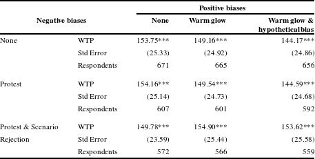
are vectors of the environmental attribute levels projected under the TMDL and baseline scenarios. Plugging in the coefficient estimates from Model 1 suggests an annual household WTP of $154.
Annual household WTP under alternative screening criteria: model 1.

***
 $p<0.01$
, **
 $p<0.05$
, *
 $p<0.1$
. Standard errors in parentheses, calculated using the Delta Method. Underlying coefficient estimates based on Mixed logit models estimated using 1000 Halton draws, and where standard errors clustered at the respondent level.
The sensitivity of this result to the screening criteria used to identify and eliminate respondents exhibiting potential biases, as discussed in Section 3, is examined next. We follow an approach similar to Banzhaf et al. (Reference Banzhaf, Burtraw, Evans and Krupnick2006), creating a matrix that incrementally applies more stringent criteria for eliminating respondents exhibiting potential biases.Footnote 11 Going from left to right in Table 10, we increasingly eliminate respondents exhibiting behaviors that may bias WTP upward, and going from top to bottom, we increasingly eliminate behaviors that may bias WTP downward. The diagonal can be thought of as a roughly symmetric treatment of these counteracting biases. The results for Model 1 are shown in Table 10, and reveal little difference in the annual household WTP when we use the full sample (upper-left cell) or apply the full screening criteria to minimize potential biases (bottom-right cell). The estimates are fairly robust across all combinations of the screening criteria, varying by less than $10.
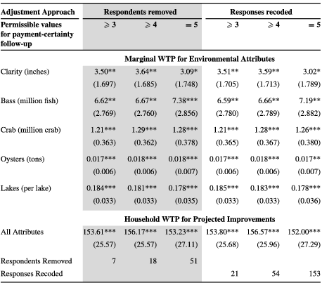
Other SP studies that control for hypothetical bias with follow-up questions typically do so with a more broadly defined question about response certainty (e.g. Blumenschein et al., Reference Blumenschein, Blomquist, Johannesson, Horm and Freeman2008; Blomquist, Blumenschein & Johannesson, Reference Blomquist, Blumenschein and Johannesson2009; Ready Champ & Lawton, Reference Ready, Champ and Lawton2010). Using similar numerical scales, other studies have tested the effect of the critical value at which a response is considered certain enough to be included in the analysis. We view our approach as an extension that asks more refined questions aimed at the sources of response uncertainty. To provide a more direct comparison to previous studies we also test the sensitivity of our results to the critical value used to screen respondents for hypothetical bias using the debriefing question regarding acceptance of the cost attribute. Results shown thus far use a value of 3 (Neutral). Below we test the sensitivity of our results to using 4 (Agree) and 5 (Strongly Agree) as the critical value. We also test the sensitivity of our results to the adjustment approach by recoding answers from a policy option to the status quo choice rather than removing them from the sample. Table 11 shows how marginal and household WTP estimates are affected if critical values of 3, 4, and 5 are used and if responses are recoded rather than removed. The figures in the table show that using the most conservative criterion for hypothetical bias and using an alternative adjustment approach makes very little difference in the WTP estimates.
Sensitivity of marginal and household WTP estimates to hypothetical bias screening criteria and adjustment approach.

***
 $p<0.01$
, **
 $p<0.05$
, *
 $p<0.1$
. Standard errors in parentheses, calculated using the Delta Method.
Similar to equation (4), for Model 2, which allows the marginal utility of the environmental attributes to differ between users and nonusers of the Chesapeake Bay and Watershed lakes, the household WTP can be calculated as:
 $$\begin{eqnarray}\mathit{WTP}^{\mathit{HH}}=\frac{\hat{\unicode[STIX]{x1D6FD}}\ln (x^{1})+\hat{\unicode[STIX]{x1D6FD}}_{\text{user}}\ln (x^{1})\cdot \text{user}-(\hat{\unicode[STIX]{x1D6FD}}\ln (x^{0})+\hat{\unicode[STIX]{x1D6FD}}_{\text{user}}\ln (x^{0})\cdot \text{user})}{(-\hat{\unicode[STIX]{x1D6FE}})}\end{eqnarray}$$
where
 $\hat{\unicode[STIX]{x1D6FD}}$
is the subvector containing the estimated coefficients on the uninteracted attribute levels,
 $\hat{\unicode[STIX]{x1D6FD}}_{\text{user}}$
is the subvector containing the estimated coefficients on the userinteracted attribute levels, and user is a vector of binary variables with the first four elements equal to one if the respondent is a user of the Bay, the fifth element equal to one if the respondent is a user of watershed lakes, and zero otherwise. The dot product operation in equation (5) indicates element-by-element multiplication.
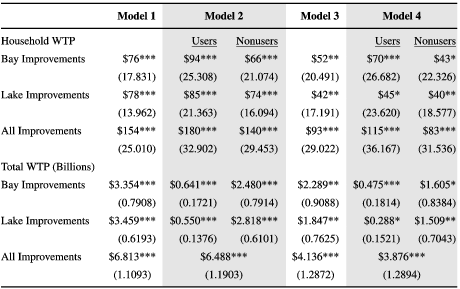
In order to calculate total WTP we first estimate the WTP of a “representative” household, taking into consideration the proportion of Bay and lake users in the population. We use data collected with the NRS because the demographic data show that the demographic characteristics of the NRS sample is more similar to the population. In addition, the potential for users to self-select into the sample is less of a concern with the shorter and cash-incentivized NRS questionnaire. To better reflect the study area population, the NRS results are weighted to account for differences in sampling intensity and response rates across geographic strata. An estimated 15.3% of the population has visited the Chesapeake Bay in the last 5 years and 14.5% visited a lake in the Chesapeake Bay watershed during that time. To estimate the WTP for a representative household, these proportions replace the zero/one elements of the user vector in equation (5). Multiplying that amount by the 44,353,441 households in the sample area provides the total WTP estimates in Table 12.Footnote 12
Annual willingness to pay for TMDL (2014 dollars).

***
 $p<0.01$
, **
 $p<0.05$
, *
 $p<0.1$
. Bootstrapped standard errors in parentheses (1000 bootstrap iterations).
The results shown in Table 12 provide several useful comparisons. First, as the regression results and MWTP estimates have already shown, when the models control for respondents’ experiences with the resources, users are willing to pay more for the anticipated improvements than nonusers, though this difference is not statistically significant. Despite the lower household WTP, about 80% of the total WTP in Table 12 can be attributed to the large proportion of nonusers. Second, conditioning on responses to debriefing questions regarding unintended factors when choosing an alternative does have an economically, though not statistically, significant impact on WTP estimates. Finally, Table 12 shows that improvements to freshwater lakes in the watershed account for about half of the total benefits. This is an important finding given that much of the watershed, and thus many of the households bearing the costs of the required management practices, is far from the Chesapeake Bay and likely to benefit less from ecological improvements in the Bay itself.
We can compare our estimates of benefits from lake improvements to the results of Van Houtven et al. (Reference Van Houtven, Mansfield, Phaneuf, von Haefen, Milstead, Kenny and Reckhow2014) who estimate household WTP for lake improvements in the state of Virginia under the same policy. Van Houtven et al. use a SP survey to estimate annual benefits of $60 per household for the 2119 lakes in Virginia affected by the TMDL. Our survey referenced more than 4200 throughout the entire watershed and our household WTP for lake improvements range from $40 to $85. There are a number of reasons we would not expect WTP to scale proportionally with the number of lakes affected, including diminishing marginal utility, variability in the projected policy impacts on lakes throughout the watershed, and typically lower WTP for out of state resources (e.g. Carson and Mitchell Reference Carson and Mitchell1989). Here it is important to emphasize that the Van Houtven study only estimates WTP for lake improvements whereas the Chesapeake Bay study included lake improvements as one of five environmental attributes, the rest pertaining to the Bay itself. Despite this difference in the scope of these two studies, the fact that these two studies independently generate very comparable household WTP estimates for lake improvements is an indication of external scope and speaks to the current state of the science in nonmarket valuation and SP methods in particular.
6 Conclusion
Improving water quality in increasingly degraded coastal estuaries requires reducing point source and nonpoint source pollution throughout the broader watershed. In large watersheds people and communities far from the estuary itself bear some of the cost of implementing pollution-reducing practices but, at the same time, are less likely to benefit directly from the improvements. The results of this study indicate that nonuse values and ancillary benefits to freshwater lakes offset the costs to these communities. The stated preference study presented in this paper captures WTP for ecological improvements in the Chesapeake Bay, freshwater lakes within the 64,000 square mile watershed, and nonuse values throughout 17 Eastern U.S. states and the District of Columbia. The projected improvements valued with the SP study are the result of an intensive integrated modeling effort based on detailed implementation plans submitted by states to meet requirements of the Clean Water Act. A hydrological model showing how the delivery of nutrients and sediment would change under the implementation plan provides data to ecological models and expert judgment allowing us to forecast changes in the populations of three highly regarded species, water clarity in the Bay, and the trophic state of watershed lakes. The extensive physical and biological modeling effort allowed the survey to present ecological endpoints as attributes in the choice questions rather than ecological inputs or compound attributes such as a water quality index. The advantage of representing the choice outcomes with endpoints is that we can ensure a consistent mapping from water quality measures to attributes that enter the household utility function directly, rather than relying on each respondent’s own understanding of these complex ecological relationships.
We find that about half of the benefits are due to improvements in freshwater lakes throughout the watershed. About 80% of the total benefits can also be attributed to nonusers of the Chesapeake Bay and freshwater lakes in the watershed. These results suggest that the inclusion of ancillary benefits and nonuse values substantially increases the net benefits of the TMDL. In addition to the clear policy implications, this study offers several contributions to the literature. First, the design of the study allows us to control for several types of biases that would otherwise skew WTP results. Second, an additional survey with a cash incentive was used to collect data from nonrespondents and provide estimates of user and nonuser populations that are less likely to be influenced by self-selection bias. Third, estimating a mixed logit model with a random coefficient on the status quo indicator variable allowed for variation in peoples’ tendency to vote for or against a policy that was not explained by other variables in the model. On average, we found a bias toward the policy options and controlled for it when estimating WTP. Fourth, using data collected with follow-up questions to the choice scenarios we found that people mistakenly considering improvements to lakes outside the watershed were generally willing to pay more for improvements in the lakes attribute and control for that potential source of bias in the econometric models. Finally, we explicitly account for ancillary benefits by including improvements in freshwater lakes as an attribute in the choice experiment, which is a significant driver of total WTP.