
Detecting the existence and effect of “audience costs” has been a fundamental quest in the study of international relations since Fearon proposed the audience cost (AC) model.Footnote 1 The AC model provides a coherent answer to several key questions in the field. It explains why state leaders can rationally go to war even if war is inefficient, why state leaders go public and provoke dramatic confrontations in communicating resolve, and why coercive threats are rare.Footnote 2 In addition, an auxiliary hypothesis—audience costs are higher in democracies than in nondemocracies—allows scholars to explain why political institutions affect state leaders’ ability to send signals and make commitments in a wide range of issues beyond military crises.Footnote 3
Despite its importance and influence, the AC model has recently met an array of theoretical skepticism and empirical challenges. Theoretically, the AC literature has not fully developed microfoundations for the origin of audience costs. Several studies propose formal models in which audience costs arise as a result of voters’ sanctions, leaders’ choices, or diplomatic sanctions.Footnote 4 However, the perennial question of why leaders are penalized for getting caught in a bluff has not been adequately answered.Footnote 5 Empirically, evidence remains thin and indirect since previous tests have been stymied by bias in observing audience costs because of selection effects in international crises.Footnote 6 Some studies, therefore, turn to experimental or indirect evidence,Footnote 7 whereas other studies look for “direct” evidence using the method of process-tracing only to find that audience costs either do not exist or have little effect in international politics.Footnote 8 In this article, however, we present empirical evidence of audience costs using observational data on crisis behavior and outcomes.
Scholars have considered direct and unbiased observation of audience costs as beyond reach because of the selection bias inherent in observational studies of strategic interactions.Footnote 9 Selection effects pose an inferential problem because each time state leaders make decisions in international crises, they have an incentive to avoid choices that would lead to outcomes with high audience costs. Consequently, leaders are less likely to incur audience costs as those costs become higher. Thus, if leaders actually back down from their public challenges, they do so probably because they suffer only marginal audience costs. As long as we study only observable audience costs that are actually incurred by state leaders, we would systematically underestimate the size of audience costs. This implies that an unbiased measure of audience costs requires observing those costs that are both incurred (hence observable) and not incurred (hence unobservable).
In this study we show how to estimate audience costs even if they are not fully observable because of selection bias. Our research design adopts a “structural” approach to uncover underlying audience costs even if leaders do not incur them. Recall that “audience costs” is the term Fearon coined to describe the payoff a state receives when it backs down in international crises relative to its payoff in the status quo. The most obvious way to measure audience costs is to estimate the underlying payoff the state would receive in each of these possible crisis outcomes. Our strategy to accomplish this task is to estimate the parameters of an underlying theoretical model that generates observable crisis behavior. This approach is known as “structural estimation” and has a long tradition in economics.Footnote 10 In political science, the recent empirical implications of theoretical models (EITM) approach has developed fully structural statistical models to estimate game-theoretic models of politics using observational data.Footnote 11 With the fully structural approach, we can estimate state preferences and, thereby, underlying audience costs using data on the choices and outcomes in crises.
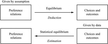
The intuition of this approach is as follows. Game-theoretic analysis deduces conflict behavior and outcomes from preferences that are given by assumption. On the other hand, statistical analysis estimates preferences from conflict behavior and outcomes that are given by data. For example, an equilibrium of a discrete choice game states that if the expected payoff of a public challenge is at least as good as the payoff of the status quo for a state, then the state will choose to make a public challenge. Empirically, since we observe the state's decision to make a challenge (or not to), we can estimate what payoffs would make this observed outcome most likely if the equilibrium had generated the data. Because we model payoffs as a combination of covariates and coefficients in the statistical analysis, the maximum likelihood estimation of coefficients gives us an empirical measurement of payoffs. Moreover, because the equilibrium in this game generates strategic selection and because we derive our statistical model from this equilibrium, our estimates of the payoffs fully take into account selection effects by internalizing them.
We report our structural estimation of a canonical crisis bargaining game. Our analysis uses the Coercive Diplomacy Database (CDDB), a new collection of data on coercive bargaining in the interwar period (1919–39).Footnote 12 Our findings provide an empirical foundation for the AC model along four dimensions:
-
• Existence. Audience costs are said to exist if the payoff that a state receives when it backs down after making a challenge is less than its payoff in the status quo. Estimating these payoffs, we show that the existence of audience costs is statistically significant and robust against various empirical specifications of these payoffs. Because the AC model does not presume any specific way in which leaders incur audience costs, our evidence is of a generic form, free of any specific source of the costs.
-
• Regime type. Our evidence for the existence of audience costs is upheld for a wide range of regime types including democracies and nondemocracies alike. This result is consistent with the claim that audience costs exist even in nondemocracies.Footnote 13 We also test, and find evidence for, the widely accepted Fearon conjecture that audience costs are on average higher in democracies than in nondemocracies.
-
• Magnitude. We find that audience costs can at times be so high that going to war can be preferable to backing down. Our estimation indicates that the magnitude of audience cots is greater than the value for war on average, though the two quantities are not statistically distinguishable. This implies that the political cost of backing down after making a challenge can be enormous for some leaders but not for others. This result gives support for the plausibility of a core argument of the rationalist literature.Footnote 14
-
• Coercive effect. Our analysis demonstrates that audience costs have nonnegligible impacts on crisis behavior. The target state is more likely to capitulate if the challenging state has higher audience costs. This effect is also substantively significant relative to a common indicator of states’ bargaining power—that is, their value for war. Our finding provides evidence against recent claims that audience costs have little effect on crisis behavior.Footnote 15 Moreover, our analysis reveals that selection effects are indeed at work, implying that the critics’ claims that downplay the importance of audience costs result from their research designs that overlook selection bias.
A Common Audience Cost Model
There are two classes of crisis models in which scholars assume that audience costs exist. The first is Fearon's original model based on a war-of-attrition game, where audience costs increase at possibly differing rates as a crisis escalates. The second is based on a canonical crisis-bargaining game, where leaders incur differing levels of audience costs if they back down in the face of the adversary's resistance.Footnote 16 Note that these classes of models are equivalent in a one-shot situation because the distinction between the rate and the level of audience costs is immaterial unless bargaining takes place over multiple stages. Since nearly all previous tests of audience costs invariably adopt a single-shot crisis game, we also use the crisis game as our underlying theoretical model to facilitate comparison with previous findings.Footnote 17
The Model
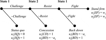
The game has the structure depicted in Figure 1. Two states, State 1 and State 2, are in a dispute over some international good in the shadow of armed conflict. The value of the good to both is normalized to 1. This good belongs to State 2 in the status quo. In the event that war occurs, State 1's payoff is given by its expected value for war w
1 = p − c
1, where p
 $ \in $
[0, 1] and c
1 ≥ 0 represent State 1's probability of victory and expected costs, respectively. Notice that the costly lottery assumption underlies the definition of war payoffs. State 2's war payoff is given by w
2 = 1 − p − c
2. States are incompletely informed about each other's relative war costs. Nature randomly selects c
1 and c
2 from independent distributions on intervals [0,
 $\bar c$
1] and [0,
 $\bar c$
2], respectively. Thus, the w
i
 $ \in $
[w
i
,
 $\bar w$
i
] are distributed according to the cumulative distribution function F
i
(x) = Pr(w
i
≤ x), whose support is [
 $p - {\bar c_1}$
, p] for State 1 and
 $\left[ {1 - p - {{\bar c}_2},\; 1 - p} \right]$
for State 2. Each state observes its own value for war w
i
, but neither observes the other's w
j
, j ≠ i. The probability distributions are common knowledge, so each state forms precrisis beliefs about w
j
as well as the posterior belief after observing the choices made by the other state.
Crisis games with audience costs

A crisis begins with State 1's decision to challenge State 2 for possession of the good. If challenged, State 2 either concedes or resists. If State 2 concedes, then the good is transferred to State 1 and the game ends. In this concession outcome State 1 obtains the value for the good, which is 1, and State 2 not only loses the good but also incurs some political cost, receiving the payoff of − a 2 < 0. If State 2 resists, on the other hand, State 1 must decide whether to back down or fight. If State 1 fights, war occurs. In the event that State 1 backs down after State 2 resists, the status quo (SQ) ante remains so that State 1 receives the payoff of 0 and State 2 keeps the SQ payoff of 1. Additionally, State 1 also pays some additional political costs, or audience costs, equal to a 1 > 0. Hence, State 1 derives the payoff of − a 1 < 0 from this back-down (BD) outcome.
Definition (audience costs)
Audience costs are the cost that State 1 incurs if it backs down, relative to its status quo payoff. We say audience costs exist if and only if u 1 (BD) < u 1 (SQ).
Given this definition, to detect the existence of audience costs, we must uncover this payoff relation in the observational data. Note that this common definition does not restrict the source of audience costs to domestic or international audiences. Nor does it specify where audience costs come from. The common AC model, as it stands, is agnostic about any specific mechanisms through which state leaders incur such costs. Although Fearon's seminal work justifies why electoral accountability might be a plausible mechanism, the model has nothing that connects regime type to crisis behavior.Footnote 18 Although several studies propose various plausible mechanisms through which those costs may be paid, there is no consensus among authors of theoretical models. The gist of the AC model, which scholars agree on, is that there is some nonzero political costs that State 1 must pay when its bluff is called so that u 1(BD) < u 1(SQ). We use this minimalist definition.
Equilibrium
We derive the perfect Bayesian equilibrium to this game in the appendix. The full range of information revelation—separating, semi-separating, and pooling—occurs in the equilibrium, depending on the relative magnitude of audience costs for State 1. If State 1 has sufficiently high audience costs (that is, a
1 ≥
 $\bar a$
), the signal fully separates State 1 types in terms of their resolve (or lack thereof).Footnote
19
If, on the other hand, State 1's audience costs are not very high (that is,
 $a_1 \lt \bar a_1 $
), they allow irresolute types to engage in bluffing behavior and to run the risk of backing down. This results in the semi-separating equilibrium. If the audience costs for State 1 are very low (that is,
 $a_1 \lt \tilde a_1 $
), the costs cannot offset the irresolute types’ temptation to gamble so that all types of State 1 will make a threat. This pooling signal conveys no additional information about State 1's resolve so that no learning occurs for State 2.
Strategic Selection
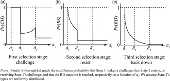
At the core of the AC mechanism is strategic selection because it determines the size and the observability of audience costs.Footnote 20 The equilibrium shows that crisis behavior is shaped by the relative magnitude of audience costs for State 1. Figure 2 illustrates how, as the crisis unfolds in three stages, the equilibrium selects State 1 out of equilibrium escalation according to the size of audience costs.
Equilibrium behavior and selection effects

At the first stage of the game, State 1 will be more prudent and hence less likely to issue clear military threats if State 1 faces higher audience costs. This is because, as Fearon suggests, the risk of getting “locked” into crisis escalation makes State 1 with high audience costs more cautious about initiating threats.Footnote
21
As a consequence, as panel (a) in Figure 2 shows, the probability that State 1 makes a threat drastically decreases as audience costs become higher than the first threshold
 ${\tilde a_1}$
.
At the second stage where State 2 decides whether to resist, State 2's (conditional) probability of resistance also monotonically decreases as a 1 increases.Footnote 22 In consequence, the probability that the final decision node is reached gets even lower as audience costs increase. Panel (b) in Figure 2 describes this second-stage selection effect: the probability that State 1 gets to decide whether to fight or back down decreases as a 1 increases.
Once the third stage is reached, State 1 is also increasingly less likely to back down as it faces higher audience costs. Since audience costs can only be observed when State 1 backs down along the equilibrium path, higher audience costs make it extremely less likely that State 1 will incur those costs. In fact, as panel (c) indicates, audience costs will never arise in equilibrium if they are sufficiently high, that is, a
1
 $\; \ge \; \bar a$
1; the vast majority of audience costs that arise in equilibrium are likely to be small, that is,
 ${a_1} < {\tilde a_1}$
.
Strategic selection, therefore, occurs at each of the three stages of crisis initiation and escalation. This equilibrium behavior has the following implication for empirical investigation:
Implication (selection bias)
The audience costs that are possibly observable are likely to be small, whereas higher audience costs are unobservable in data on international disputes.
Inference Problems in Detecting Audience Costs
It is difficult to overstate the importance of strategic selection bias in adequately interpreting data and designing empirical tests. To highlight the inferential problems in testing the AC model, we review the previous empirical investigations.
Process Tracing Case Study
Snyder and Borghard offer one of the first case studies to evaluate the AC model. They find that “domestic audience costs mechanisms rarely play a significant role.”Footnote
23
This would certainly be an important finding if true. However, they misinterpret the findings from their case studies because they underestimate threats to causal inference posed by selection bias. For example, the authors note that strategic selection does not cause inferential bias as long as “leaders … fail to carry out their threats in a crisis, and the consequences of those empty threats can in fact be observed.”Footnote
24
But selection bias is not about whether empty threats and their consequences are observable. The real problem is whether those observable outcomes represent the true distribution. As panel (c) in Figure 2 indicates, although the BD outcome can indeed occur in equilibrium, the observable distribution of audience costs is truncated above
 $\bar a$
1 and the vast majority of states that back down face low audience costs (
 ${a_1} < {\tilde a_1}$
). This implies that the leaders who actually make it to the BD outcome are likely to be those who suffer little punishment for failing to follow through on their threats. Hence, Snyder and Borghard's finding about the lack of “examples of called bluffs leading to domestic punishment of democratic leaders” is not evidence against the AC model but is actually consistent with it.Footnote
25
Similarly, panel (a) in Figure 2 indicates that the probability that State 1 makes a threat drops if audience costs are sufficiently high (that is,
 ${a_1} \ge {\tilde a_1}$
). Hence, Snyder and Borghard's finding about the rarity of clearly committing threats is not evidence against the AC model either. This misinterpretation is not uncommon.Footnote
26
Downes and Sechser also claim that the rarity of clear military threats is problematic for assessing democratic credibility and, by extension, AC mechanisms.Footnote
27
This claim misplaces the nature of selection effects—indeed, this rarity is not only predicted by AC mechanisms but also a reason for scholars to propose the concept of audience costs in the first place.Footnote
28
Indirect Statistical Tests
The partial observability of audience costs has led scholars to look for indirect evidence of the costs by testing observable implications on how political regimes affect states’ behavior in international disputes.Footnote 29 Based on the belief that we cannot directly observe or estimate preferences, indirect tests are intended to interpret crisis behavior as a manifestation of preferences.Footnote 30 However, this empirical strategy invokes the problem of “revealed preferences.” Frieden notes that inferring preferences from observation risks confounding preferences with their effect because observed behavior may result “only partially, perhaps misleadingly, from underlying preferences.”Footnote 31 The strategic interdependence of choices in international disputes ensures that the preferences revealed through observed behavior are almost always misleading.
Moreover, since this research design lacks a measure of audience costs, scholars often use a democracy index to approximate audience costs. However, this practice is based on a potentially problematic untested conjecture about the correlation between regime type and audience costs. Audience costs are essentially expected costs that are a function of the severity of punishment and the probability of being punished. Although authoritarian leaders are less likely to be punished politically than are democratic leaders, they are often subject to harsher punishments when they leave office, at which point they may face imprisonment or even assassination.Footnote 32 The expected cost of a failed policy for authoritarian leaders can thus be significantly higher than is commonly conjectured. This reasoning suggests that domestic audience costs may not be confined to democratic regimes. Weeks has recently demonstrated that some dictators can also raise these costs in a dispute that generates the kind of impacts on crisis outcomes that the AC model predicts.Footnote 33 Since a large volume of empirical research adopts this conjecture, it is crucial to find its evidence.
Survey Experiments
Survey experiments are the state-of-the-art strategy for testing AC mechanisms because they are designed to overcome the issues of selection bias and the partial observability of preferences. These experiments measure audience costs in terms of approval ratings embedded in opinion surveys and demonstrate evidence of those costs even though state leaders do not incur them.Footnote 34
Although innovative and rigorous, the external validity of audience costs reported in the existing survey experiments is in doubt for at least two reasons.Footnote 35 First, the choice of “approval rating” as the form of audience costs may inflate the size of the costs. For example, consider two ways in which democratic leaders may incur audience costs: electoral removal from office and unfavorable approval rating. It is more likely for a leader to receive unfavorable approval ratings than to lose an election, so the size of audience costs can be systematically higher in the form of approval rating than in the form of electoral removal. Indeed, gauging approval ratings of US presidents in simulated crisis scenarios, Trager and Vavreck find that audience costs are larger than the cost of fighting a war.Footnote 36 On the other hand, focusing on other types of domestic punishment, Snyder and Borghard find little evidence of audience costs.Footnote 37 Similarly, Goemans suggests that the likelihood that leaders get electorally defeated is higher than the likelihood of severe punishment such as exile or death.Footnote 38 Scholars may reach different conclusions on the existence or magnitude of audience costs, depending on the form of audience costs. To enhance external validity of inference, therefore, it is important to measure audience costs of a generic form without any restrictive focus.
Second, the survey treatments are designed to present leaders’ decisions to make threats and their consequences explicitly to their respondents. Gartzke and Lupu argue that this design is not plausible because the public is not generally knowledgeable about foreign policy.Footnote 39 Holsti also notes that the average American citizen is remarkably uninformed about even the most elementary aspects of international affairs.Footnote 40 Moreover, scholars have shown that policy-makers often evade audience costs by making vague or secret threats that would enable them to obfuscate whether they failed to follow through on their commitments.Footnote 41 Since the information environment for the respondents in the experimental designs is too salient to be true in the real world, we suspect that real-world audience costs are smaller than those appearing in survey experiments.
Empirical Strategy
To detect the existence and size of audience costs, we estimate the costs per se, rather than interpret conflict behavior as a manifestation of the underlying audience costs. As noted earlier, audience costs are defined as the difference between the payoffs that a state receives if it backs down after making a challenge and in the status quo, that is, u 1(BD) − u 1(SQ) < 0. Consequently, our goal of the empirical analysis is to infer each of these underlying payoffs that states would receive in the crisis game depicted in Figure 1 and test the statistical significance of the difference among them.
Structural Estimation Approach
To infer payoffs in the underlying crisis game, we use the “fully structural estimation” approach, a well-established approach to estimate the parameters of theoretical models from data.Footnote 42 The structural approach differs from the common “reduced-form” approach in that it estimates a theoretical model itself rather than testing comparative static predictions in isolation from the theoretical model. Following the seminal work by Signorino on the use of Quantal Response Equilibrium, the recent EITM movement spurred the development of structural estimation of game-theoretic models of politics based on Perfect Bayesian Equilibrium.Footnote 43
More specifically, we derive a statistical model from the crisis game and the perfect Bayesian equilibrium therein. By estimating this resulting statistical model, we obtain the structural parameters of the model, including the payoffs. As Figure 3 illustrates, theoretical analysis deduces (probability distributions of) crisis behavior and outcomes from state preferences given by assumptions and an equilibrium describes this deduction. Then, statistical analysis does exactly the opposite: we estimate state preferences from (a frequency distribution of) observed behavior and outcomes according to a statistical model of the same equilibrium. For example, the perfect Bayesian equilibrium to the crisis game states that if State 1's expected payoff from a challenge (CH), u 1(CH), is greater than or equal to its SQ payoff, u 1 (SQ), State 1 is expected to make a challenge in equilibrium. With structural estimation, in turn, we infer that State 1's choice of CH is caused by the preference relation: u 1 (CH) ≥ u 1 (SQ). In estimating our statistical model, therefore, we ask “given the observed crisis outcomes in data, what combination of payoffs would make this observation most likely according to the perfect Bayesian equilibrium?” Thus, statistical inference of preferences from conflict outcomes amounts to the “reverse reasoning” of an equilibrium logic that derives conflict outcomes from preferences.
Inferring the perferences

One nice feature of the structural estimation approach is that we can estimate the payoffs of every outcome for each state as long as the four outcomes in the crisis game have non-zero frequency. Once we recover the underlying payoffs for States 1 and 2 from data, we can infer the size of audience costs for each observation even if, for example, State 2 does not back down in some specific observation. Estimating counterfactual quantities is not new; for example, it is analogous to inferring an expected value of 1 for an observation that has an actual value of 0 in a conventional logit or probit model. This is the advantage over historical case studies because they cannot infer the size of audience costs if there is no clearly defined back-down observation when the underlying audience costs are large. Moreover, since our estimate of audience costs does not depend on any particular form or source from which audience costs arise, it will be free of the type of bias in inference that the previous studies suffer.
Statistical Model of Audience Costs
Intuitively, our statistical model of audience costs embeds a likelihood function of a binary choice at each decision node in the theoretical model (Figure 1). We briefly explain each of the steps we take to construct this model: (1) translate the theoretical model to a statistical model; (2) solve the statistical model for the perfect Bayesian equilibrium; and (3) derive a log-likelihood function as a multinominal logit or probit and obtain the maximum likelihood estimates.
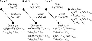
First, to derive a statistical model from the theoretical model, we assume that all the payoffs are a linear combination of a systematic component that is common knowledge and a stochastic component that represents private information. The systematic component of a payoff, in turn, is a function of covariates and coefficients to estimate. For example, State 1's payoff for the stand-firm (SF) outcome is defined as follows:
 $$\eqalign{u_1 \left({SF}\right) & =\;\bar u_1 \left({SF}\right) + \; \varepsilon _{SF_1 } \cr & = X_{SF_1 } \beta _{SF_1 } + \varepsilon _{SF_1 } ,}$$
where
 $\bar u_1 \left( {SF} \right)$
, ε
SF1, X
SF1, and β
SF1 respectively denote the average value of u
1(SF), the stochastic term of u
1(SF) (which is drawn from a normal distribution with mean 0), a set of the covariates for u
1(SF), and a vector of coefficients that we estimate using maximum likelihood. This setup implies that, unlike the theoretical model, all outcomes occur in equilibrium with positive probabilities because of unbounded stochastic shocks included in each payoff.Footnote
44
The redefined payoffs in the statistical model of audience costs are shown in Figure 4.
Statistical model of audience costs

Second, we derive the equilibrium probabilities of the four outcomes in the statistical model. These probabilities are a product of choice probabilities that State 1 and State 2 make at each decision node. For example, the probability of the SF outcome, Pr(SF), is given by the probability State 1 initiates a challenge, Pr(CH), the probability that State 2 resists, Pr(RS|CH), and the probability State 1 fights Pr(SF|CH). The probability of decision is dictated by the perfect Bayesian equilibrium. For example, the probability that State 1 fights is given by the probability that the SF payoff is at least as good as the BD payoff for State 1, that is, Pr(SF) = Pr(u 1(SF) ≥ u 1(BD)). In the appendix, we detail the equilibrium probabilities of the outcomes, Pr(SQ), Pr(CD), Pr(BD), and (SF).
Third, we construct the log-likelihood function as a multinominal discrete choice model by summing up the equilibrium log-likelihoods of four outcomes as follows:
 $${\rm ln}\; L\;= \mathop \sum \limits_{i = 1}^N [Y_{{\rm SQ}_i } {\rm lnPr}\left({SQ_i }\right) + Y_{{\rm CD}_i } {\rm lnPr}\left({CD_i }\right) + Y_{{\rm BD}_i } {\rm lnPr}\left({BD_i }\right) + Y_{{\rm SF}_i } {\rm lnPr}\left({SF_i }\right)],$$
where Y
z denotes a binary variable that represents a crisis outcome
 $z \in \left\{ {SQ,} {CD,BD,SF} \right\}$
.
The structural estimation of the theoretical model boils down to this log-likelihood function, which is exactly the same as the log-likelihood function of conventional discrete choice models, except that the outcome probabilities (for example, Pr(SQi )) are determined by the perfect Bayesian equilibrium. Note that these outcome probabilities are a function of the choice probabilities (for example, Pr(SF)), which in turn are a function of the relative payoffs (for example, Pr(u 1(SF) ≥ u 1(BD))).
Since each payoff is a linear function of tangible covariates and their coefficients (for example, X SF1 β SF1), we can estimate a set of coefficients, the βs, for each payoff that maximizes the likelihood of the observed outcomes. Using these β coefficients, we can recover payoffs (and hence audience costs) and infer how, for example, the level of democracy of a state affects the size of its audience costs.
Payoff Specification
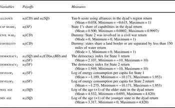
Since we estimate the coefficients (βs) using a set of covariates (Xs), we need to specify the Xs that determine each player's payoff for each crisis outcome. We derive the empirical specification of the payoffs from the theoretical specification in Figure 1 and common interpretation of those payoffs. To do so, we minimize the number of control variables outside of the theoretical model, since our goal is to estimate the theoretical AC model itself—that is, to characterize the AC model with data. Table 1 summarizes the assignment of covariates to each payoff.
Explanatory variables

Notes: The source for democracy
i
,
 $i \in \left\{ {1,2} \right\}$
is the Polity IV data set and for the rest of variables is the Correlates of War project.
The war payoffs in the theoretical model are given by u 1(SF) = p − c 1 and u 2(SF) = 1 − p − c 2, both of which are a function of the probability that State 1 prevails in armed conflict and the cost of fighting. The probability of winning, p, in the costly lottery formulation of the war outcome is commonly interpreted as the relative share of military capabilities.Footnote 45 We use cap share 1 to measure State 1's share of capabilities in the dyad. The cost of war, c i , i = 1,2, is often understood to be smaller if state i is economically more developed because superior military technologies reduce the relative cost of war. We use develop 1, i = 1,2, to measure the material (or financial) cost of war for each state. In addition to material capabilities, the democratic peace literature suggests that regime type influences political costs and political will (that is, resolve) to go to war.Footnote 46 We therefore include democracy 1, i = 1,2, as another proxy for c i in the equation of u i(SF).
The BD payoff for State 1 in the theoretical model is u 1(BD) = 0 − a 1, where State 1 not only fails to obtain the disputed good but also suffers audience costs. To evaluate Fearon's conjecture that audience costs are higher in democracies than in nondemocracies, we use democracy 1 to measure a 1.
We normalize State 2's BD payoff, u 2(BD), because model identification requires that we normalize the constant in at least one of the payoff specifications for each player. We place this restriction on u 2(BD) without loss of generality because the BD outcome is not an immediate result of State 2's deliberate decision and it is equivalent to the SQ outcome from State 2's perspective.Footnote 47
The SQ payoffs in the theoretical model are given by u 1(SQ) = 0 and u 2(SQ) = 1. The constant for the equation of u 1(SQ) is normalized to 0 because of the identification requirement. We choose to normalize u 1(SQ) because this payoff is also normalized in the theoretical specification and because State 1 does not possess the disputed good in the SQ outcome (as in the BD outcome).Footnote 48 We drop u 2(SQ) from our estimation because it never determines equilibrium choices or the calculation of the equilibrium probabilities—whether the status quo is maintained or challenged is solely decided by State 1 in the game. There is nothing to infer about u 2(SQ).
The concession payoffs in the theoretical model are u 1(CD) = 1 and u 2(CD) = 0 − a 2. Since the theoretical model is of little help for our specification choice, we include three covariates that control for strategic factors that may influence the payoffs that each state may derive from the concession outcome. First, the value of the disputed good is influenced by the similarity of strategic interests between the states. We include alliance to control for the similarity of alliance portfolio in a disputing dyad. The historical record shows that a number of international disputes occur when the target country is involved in civil wars.Footnote 49 This implies that civil wars influence the strategic assessment of the disputed good for both states because they make the target country vulnerable to the coercive pressure from other states. Thus, civil war 2 indicates whether State 2 is involved in a civil war. Finally, Huth and Allee show that countries with a shared border have higher risks of dispute escalation.Footnote 50 We use contiguity indicating whether two states share a border.
Note that some political or diplomatic costs, − a 2, incurred by State 2 in the concession outcome are also considered some sort of “audience costs.” Although different than the original formulation, it would be interesting to examine if such audience costs for State 2 are also associated with its regime type. Hence, we estimate an alternative model with democracy2 for u 2(CD) as part of the robustness check.
A caveat is in order. Note that the empirical specification of the payoffs, or the choice of which covariate to be included in which payoff equation, does not significantly alter the empirical implications that we draw from the estimation result. This is because the payoffs in both theoretical and empirical models are all relative and, thus, all covariates affect all the payoffs directly or indirectly.Footnote 51 For example, even if develop1 is included only for u 1(SF), it still affects all the decisions in the model. This is true in the underlying theoretical model as well as our empirical model. Since the decision to fight depends on the relative magnitude of u 1(SF) and u 1(BD) in the theoretical model, develop1 affects not only u 1(SF) but also u 1(BD) in a relative way in the empirical model as well.
Data
To estimate our statistical model in Figure 4, we analyze states’ decisions to initiate, resist, and follow through on challenges to the status quo. The existing data sets, such as the Militarized Interstate Dispute (MID) data, the International Crisis Behavior (ICB) data, and the Militarized Compellent Threats (MCT) data set, provide no information on whether the challenger followed through or backed down on its threat.Footnote 52
Our data set is based on the CDDB compiled by Schultz, Lewis, and Zucco.Footnote 53 The CDDB records episodes of crisis bargaining as it is characterized in Figure 1 for seventy-seven crises for the interwar period (1919–39) that are drawn from the ICB and MID data sets. The CDDB defines a challenge as any act that is made deliberately by a central state authority with the intent of altering the precrisis relationship between itself and at least one other state and that is backed by the threat of military force. If a challenge is identified, the CDDB maps the outcome of each crisis episode to one of the three outcomes, CD, BD, and SF, in the crisis game shown in Figure 4.
We also include a series of nonchallenge observations in which State 1 does not challenge the status quo. We use the coding rule developed by Huth and Allee and adopted by Lewis and Schultz to identify the status quo observations.Footnote 54 If a politically relevant dyad has not experienced a crisis episode for three years according to the CDDB, it is coded as an SQ outcome during that time period.Footnote 55 Hence, the unit of analysis is dyad-three-years if the outcome variable is coded as SQ and crisis-dyad if the outcome is either CD, BD, or SF. The distribution of the outcomes is SQ = 2025, CD = 35, BD = 11, and SF = 35. In addition, we employed alternative coding rules for the SQ observations by varying the time period to look for a CDDB crisis. We used three different windows (that is, one year, two years, and four years) to identify the SQ observations. We found the results to be stable and robust regardless of the coding rules.
Estimation Results
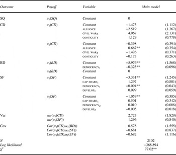
Table 2 displays the maximum likelihood estimates of the main model. We report the coefficient and standard error for the constant and covariates (if applicable) in the equation for each payoff. The χ 2 statistic suggests that our payoff specifications in the main model significantly improve on the null model in which all the coefficients are jointly restricted to 0.
Estimation result of the main model
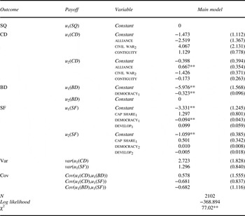
Notes: The table reports coefficient estimates with standard errors in parentheses. **p < .05.
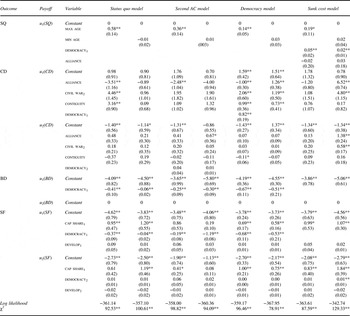
Table 3 shows the estimation result for some of the key alternative models. The status quo model controls for State 1's incentives to initiate a crisis or to maintain the status quo. An important issue that loomed large during the interwar period is the boom of the newly created states and corresponding boundary disputes in the wake of World War I. The restriction of the analysis to “politically relevant dyads” attempts to control for the opportunity for conflict; we also include two variables to the equation of State 1's SQ payoff, u 1(SQ), to control for the willingness for conflict. The first variable is max age that measures the age of the older state to control for the status quo bias, and thereby disincentives for territorial claims, of a more established state.Footnote 56 The second control is min age that measures the age of the younger state in the dyad since a new state tends to face greater territorial imperatives in this period. The result shows that min age is not statistically significant, whereas the coefficients on max age are consistently positive and significant in all the models, indicating that an older state has a stronger incentive to maintain the status quo. Estimated coefficients on other covariates (especially those for u 1(BD) and u 1(SF)) largely remain unchanged from the main model. We also assess the effectiveness of these controls in the sunk-cost model that includes other factors that may affect State 1's incentives to initiate a crisis.
Alternative specifications

Notes: The table reports coefficient estimates with standard errors in parentheses. The estimates of variance and covariance are suppressed. *p < 0.1 (two-tailed); **p < 0.05.
The second AC model adds democracy2 to the equation of State 2's concession payoff, u 2(CD). The nonsignificance of this covariate rejects the hypothesis that the political costs, or audience costs, of public concessions for State 2 are associated with its democracy score. The coefficients of key covariates in the equations for u 1(BD) and u 1(SQ) are generally consistent with those in the main model.
The democracy model includes democracy1 in State 1's payoffs for all three crisis outcomes, u 1(CD), u 1(BD), and u 1(SF). Its positive coefficient in the u 1(CD) equation is consistent with the negative coefficients for both u 1(BD) and u 1(SF). Democracies prefer that State 2 concedes because the BD outcome and the SF outcome, both of which are a consequence of State 2's resistance, are more costly for democracies.
The sunk-cost model includes democracy1 and alliance in the u 1(SQ) equation. The estimation result shows the robustness of the control variable max age in the u 1(SQ) equation, since the sign and significance of its coefficient are consistent after controlling for these confounding factors.Footnote 57 Note that since the sunk-cost model has democracy1 only in the u 1(SQ) equation, this specification is equivalent to including democracy 1 in the equation for all three crisis payoffs (u 1(CD), u 1(BD), and u 1(SF)) but forcing it to have the same effects on them. The positive and significant coefficient on this covariate has important implications for strategic incentives faced by democracies in international crises. First, democracies pay higher sunk costs, in addition to hands-tying costs, by initiating a crisis, regardless of its outcome. Thus, the sunk-cost model is more relevant to measure sunk costs than audience costs. Second, the finding that democracies incur large sunk costs in the sunk cost model is consistent with the effect of DEMOCRACY1 in other models. Specifically, it is consistent with the negative coefficients on democracy1 in both u 1(BD), and u 1(SF) equations across all the other models. Since democracies consistently incur higher costs both when they fight and back down than nondemocracies do, they find it preferable to staying out of a crisis. Moreover, recall that democracy1 also has a positive impact on u 1(CD) in the democracy model. These effects of democracy1 in the two models altogether suggest that democracies may have mixed motives in initiating a crisis. That is, although democracies have some incentive to initiate a crisis because their payoff is higher if State 2 concedes than the payoff for nondemocracies, they are nonetheless reluctant on average to initiate a crisis because they suffer more if State 2 resists.
Overall, these alternative models suggest that the estimation result of the main model is stable and consistent. The findings are robust against further alternations in the empirical specification of the payoffs and against the change in the unit of analysis for the SQ observations to dyad-year, dyad-two-years, or dyad-four-years. Consequently, the test of hypotheses concerning the existence, magnitude, and effects of audience costs are primarily based on the main model, where the selection rule for the SQ observation employs dyad-three-years.
The Existence of Audience Costs
To test the existence of audience costs for State 1, we use the estimation result to evaluate whether the payoff relation, u
1(BD) < u
1(SQ), holds in the data. In the main model, the estimated BD payoff for State 1,
 ${\bar u_1}\left({BD}\right)$
, is given by the constant of −5.967 and the coefficient of −0.323 for democracy1
. The estimated SQ payoff,
 ${\bar u_1}\left({SQ}\right)$
, is simply given by 0 because of normalization. Taken together, audience costs exist if
 $$ - 5.967 - 0.323\; \times \; {\smallcaps \rm DEMOCRACY}_1 \lt 0.\; $$
This inequality always holds because democracy1 takes values between −10 and 10. To see if normalizing the SQ payoff to 0 undermines the falsifiability of the existence hypothesis u 1(BD) < u 1(SQ), we also examine the payoff relation in the status quo model with max age. Given the estimated coefficients for u 1(BD) and u 1(SQ), audience costs exist in the status quo model if
 $$\underbrace { - 4.092 - 0.411\; \times \; {\smallcaps \rm DEMOCRACY}{_1}}_{ = {{\bar u}_1}\left({BD}\right)} \lt \underbrace {0 + 0.575\; \times \; {\smallcaps \rm MAX \ AGE}.}_{ = {{\bar u}_1}\left({SQ}\right)}$$
When democracy1
= −10, the estimated BD payoff, u
1(BD), is 0.018 so this inequality would not hold if max age < 0.031. However, since the sample minimum of max age is 0.693, this inequality holds for democracy1
= −10. When democracy1
≥ −9,
 ${\bar u_1}\left({BD}\right)$
is strictly less than
 ${\bar u_1}\left( {SQ} \right)$
regardless of max age. Consequently, the payoff relation
 ${\bar u_1}\left( {BD} \right)\; \lt \; {\bar u_1}\left( {SQ} \right)$
always holds in the status quo model as well.
Since the estimated payoff relations in equations (1) and (2) are based on the estimated constants and coefficients, it is possible that these payoff relations result from random chance. We thus examine whether the estimated payoff difference,
 ${\bar u_1}\left({BD}\right) - {\bar u_1}\left({SQ}\right) \lt 0$
, is statistically significant by generating the confidence intervals at 95 percent for the difference between the two payoffs, using bootstrapping methods.Footnote
58
If the upper bound of the confidence interval is greater than 0, audience costs are not statistically significant (that is,
 ${\bar u_1}\left({BD}\right) - {\bar u_1}\left({SQ}\right) \gt 0$
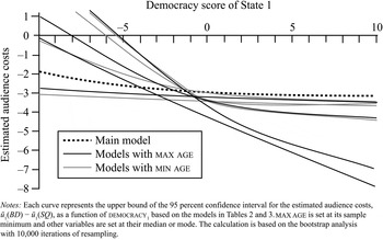
). Figure 5 summarizes the 95 percent upper bound of the confidence interval for the models in Tables 2 and 3. The dotted curve is for the main model, the solid curves in black are for the models with max age in the u
1(SQ) equation, and the gray curves are for the models with min age. To provide a “least likely” case to test the existence hypothesis, max age is set at its sample minimum.
The existence of audience costs

Figure 5 shows that in some specifications (for example, main, status quo, and sunk-cost models), the confidence upper bound is strictly negative, whereas in other specification (for example, second AC and democracy models), the confidence upper bound exceeds 0 for a sufficiently low level of democracy for State 1, that is, for democracy1 ≲ − 5. This observation holds both in models with max age and min age.Footnote 59 This result suggests that the payoff relation u 1(BD) > u 1(SQ) is statistically significant and thus state leaders of a wide range of regime types, including democracies and nondemocracies alike, will incur audience costs on average if they back down in a military crisis. The existence of audience costs is especially robust unless State 1 is highly nondemocratic.
The figure also provides supportive evidence for Fearon's conjecture that audience costs are higher in democracies than in nondemocracies. Indeed, the coefficient on democracy1 for u 1(BD) is consistently negative and statistically significant in all relevant models, implying that State 1's BD payoff decreases as State 1 becomes more democratic. This result offers an empirical foundation for a large volume of applied research that uses the level of democracy as a substitute for the existence or size of audience costs.
The Magnitude of Audience Costs
Fearon shows that high audience costs can explain “how and why states might rationally come to conclude that fighting [is] preferable to … concessions.”Footnote 60 Testing this core tenet of rationalist explanations for war in survey experiments, Trager and Vavreck find that waging war is more profitable than backing down (that is, u 1(BD) < u 1(SF)) even if the war is unsuccessful.Footnote 61 However, as we have indicated earlier, their choice of approval rating as a form of audience costs may inflate the size of the costs relative to other forms such as electoral defeat and exile. Moreover, political knowledge about crisis behavior and outcomes available to political audiences is more limited in the real world than in survey experiments.Footnote 62 Thus, we also test this claim by estimating the magnitude of “average” audience costs of a general form without assuming their particular form based on observational data on crises in 1919–39.
In the context of our statistical model, the hypothesis that audience costs can be so high that the decision to go to war is preferable to backing down is falsifiable in the form of the following payoff relation:Footnote 63
 $$\eqalign{& {{\bar u}_1}\left({BD}\right) - {{\bar u}_1}\left({SQ}\right) \lt {{\bar u}_1}\left({SF}\right) - {{\bar u}_1}\left({SQ}\right) \cr & \hskip41pt{{\bar u}_1}\left({BD}\right) \lt {{\bar u}_1}\left({SF}\right).\;} $$
In the main model (Table 2), the constant and democracy1 in the equation of u 1(SF) are statistically significant, whereas cap share1 and develop1 fall short of the conventional significance level. Then, the estimated payoff relation is as follows:
 $$\underbrace { - 5.976 - 0.323\; \times \; {\smallcaps \rm DEMOCRACY}{_1}}_{ = {{\bar u}_1}\left({BD}\right)} \lt \underbrace { - 3.331 - 0.094\; \times \; {\smallcaps \rm DEMOCRACY}{_1}}_{ = {{\bar u}_1}\left({SF}\right)}.$$
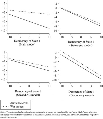
This inequality holds for any value of democracy 1. Figure 6 visually displays the relative magnitudes of estimated audience costs (in the solid line) and estimated war values (in the dotted line) as a function of democracy 1 based on the four models: main, status quo, second AC, and democracy with max age. Note that each panel shows the case where the difference between these two quantities is the largest (that is, where cap share1 and develop 1 are at their sample maximum).
Magnitude of audience costs and war values

Although the difference between audience costs and war values appears substantial in the main model, the bootstrapped confidence intervals (not shown in the figure) indicate that the difference is not statistically significant at the 95 percent level for any value of democracy 1. In three other models, the estimated audience costs do not appear to be substantively different than the war values. The bootstrap analysis confirms that the two quantities are statistically indistinguishable for any democracy 1 values in any of the models. We also found this result—that audience costs and the values of fighting are statistically equivalent—to be consistent and robust with any coding rules for the defining SQ observations and with the models with min age.
With this result, we cannot confirm Trager and Vavreck's experimental finding that waging war is significantly more profitable than backing down. Nor does it indicate that backing down is more profitable than going to war. That is, although the magnitude of audience costs is not statistically different from the size of war values for State 1 on average, state leaders can at times face substantially large audience costs in international crises. This result supports the plausibility of rationalist explanations for war, suggesting that some state leaders engaged in a crisis between 1919 and 1939 may have faced large audience costs that compelled them to abandon negotiated settlements (such as the BD outcome) and bring their nations to war.Footnote 64
However, it is important to notice that this result does not suggest that state leaders will always incur such large audience costs or that large audience costs always lead leaders to go to war. This is because both States 1 and 2 have a strong incentive to avoid outcomes that entail large audience costs. We have demonstrated that this selection effect is at work in sequential choices in crises both theoretically in Figure 2 and empirically, for example, with the negative and statistically significant coefficient on democracy 1 for u 1(BD) in Tables 2 and 3.
The Effects of Audience Costs
The AC model predicts that State 2 concedes at a higher rate when State 1 challenges the status quo if State 1 faces higher audience costs (see panel (b) in Figure 2). Audience costs exert coercive effects because they amplify the efficacy of State 1's threat. Note that if State 1 faces sufficiently high audience costs, it can no longer rationally back down from its threat. Consequently, once State 1 establishes the fait accompli by making a threat in the face of high audience costs, State 2's concession becomes the only feasible peaceful settlement at this point in the crisis game, so that State 2 is solely responsible for avoiding armed conflict.Footnote 65 In this way, high audience costs increase the credibility of the threat and thereby reinforce coercive pressure on State 2 to capitulate. All else equal, State 2 is expected to be less likely to resist in a crisis as the size of audience costs for State 1 increases.
Against this prediction of the AC mechanism, there are two rival hypotheses regarding the effect of audience costs and, by extension, democracy. The first of these is the null hypothesis, which posits that “audience costs … have at most a very small effect on crisis behavior.”Footnote 66 Snyder and Borghard reach this conclusion by studying the only cases where challengers decided to back down from their challenge. Downes and Sechser also reach the same conclusion by restricting the analysis to the cases where challengers did not shy away from making a clearly committing threat.Footnote 67 The second rival hypothesis is a democratic constraint argument, which asserts that democratic accountability makes the decision to go to war costly for democratic leaders, so that democratic leaders are less likely to wage war than nondemocratic counterparts.Footnote 68 Since higher audience costs are associated with democracy and democratic institutions are transparent, this argument would imply that high audience costs would help State 2 infer that State 1 is willing to back down if State 2 resists. Consequently, State 2 is more likely to resist as audience costs for State 1 increase.
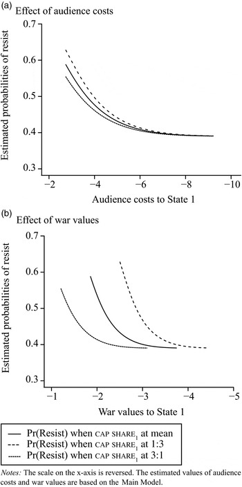
We use our estimates of audience costs to reexamine their coercive effect on State 2's decision to resist in crises. Panel (a) of Figure 7 graphs the estimated probability that State 2 resists following State 1's challenge as a function of estimated audience costs based on the main model. To help clarify the substantive significance of this effect, we compare it with the effect of war values, which is displayed in panel (b) of Figure 7. We choose this comparison since a state's bargaining power is typically interpreted as its outside option, that is, the value for war.Footnote 69 Further, since the 3:1 rule in the balance of power has important implications for the prospect for victory, we depict these effects when the capability balance is 1:3 and 3:1 between States 1 and 2 with the dashed and dotted curves, respectively.Footnote 70
Effect of audience costs on probability of resist

The results show that audience costs for State 1 have a negative impact on the likelihood that State 2 resists in international crises, which is statistically significant at the 95 percent level.Footnote 71 As Figure 7 shows, this impact is also substantively significant, since the size of these effects are roughly the same with that of war values. For example, as audience costs increase from −3, which is the minimum, to −9, which is the maximum, the probability that State 2 resists decreases roughly by 20 percent. On the other hand, as the war value for State 1 changes from −2 (maximum) to −4 (minimum), the probability of resistance also drops by 20 percent. In addition, panel (b) indicates that the shift in the capability balance from 1:3 (dashed curve) to 3:1 (dotted curve) produces at most a 25 percent change in the probability that State 2 resists when State 1's war value is roughly −2.5. These results suggest that the effect of audience costs is as sizeable as the factors that are traditionally emphasized by realists such as military power and expected values of war.
Our statistical evidence supports the AC model, rejecting the null and democratic-constraint hypotheses. We obtain this result because our analysis accounts for selection effects at all stages in a crisis. State 1's decision to back down and State 2's decision to resist are not the only decisions that are affected by audience costs; the costs also shape State 1's initial decision to make a challenge. Snyder and Borghard and Downes and Sechser cannot reject the null hypothesis because their research is designed to observe the cases in which audience costs have only little effect.Footnote 72
Conclusion
Selection bias and other inferential problems have stymied efforts to observe audience costs directly. The lack of direct evidence of audience costs has caused skepticism about the evidentiary basis for the AC model. To fill this gap, we provide an ex ante measure of audience costs by estimating the underlying state preferences in a canonical crisis bargaining game. Since selection effects are embedded in our statistical analysis, our estimate of audience costs accounts for those costs that are both actually incurred and not incurred. With these estimated audience costs, we also find empirical evidence for several propositions and questions that are central to the study of international relations.
First, this analysis demonstrates the existence of audience costs. Our estimate of audience costs is statistically significant for a wide range of regime types, democracies and nondemocracies alike, with the exception of highly autocratic regimes.
Second, our analysis shows that the magnitude of audience costs is correlated with the level of democracy. This finding confirms a working hypothesis, conjectured by Fearon and widely cited by a large number of scholars, that leaders in democracies face higher audience costs than leaders in nondemocracies do.
Third, we offer empirical evidence for a core tenet of rationalist explanations of why war occurs. We find that audience costs and war values are equivalent on average in magnitude for any regime type. This result implies that the cost of backing down after making a challenge in a crisis can be so high that war may be preferable to concessions. This may help explain why state leaders abandon peaceful settlements and resort to war.
Fourth, our result strongly indicates that audience costs cause selection effects in international crises. Audience costs make it less likely that a state backs down from a publicly issued challenge, and less likely that a state makes such a challenge in the first place. Thus, audience costs partly explain why clearly committing threats are rarely observed in international politics and why audience costs, when and if they are actually incurred and hence observed, are very small.
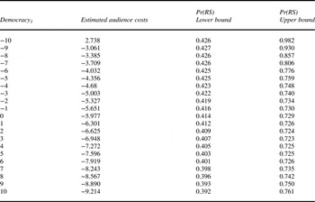
The 95 percent confidence interval for the probability that State 2 resists

Notes: The upper and lower bounds of the 95 percent confidence interval for the estimated probability that State 2 resists Pr(RS) conditional on State 1's threat are depicted in panel (a) of Figure 7. The confidence interval is obtained via the bootstrap analysis of the main model for the case of two-tail test. All variables are held constant at their respective mean values.
Finally, we show that the target state is less likely to respond militarily as audience costs for the challenging state increase. This effect is substantively nontrivial in comparison with the effect of the war values. The result suggests that audience costs render bargaining leverage that influences the course and outcome of international crises.
These findings are robust across all of the alternative specifications that we tested with different coding rules for the status quo observations. Altogether, these results provide empirical evidence for the AC model.
Nevertheless, much further work remains to be done. In particular, the common theoretical model that underlies our empirical analysis in this article is agnostic about the source of audience costs, or the way in which the costs are incurred. All that we have shown in this article is that a state incurs, or would incur, some additional nonzero costs, free of any specific form. As Schultz writes, audience costs are like the “dark matter” of international relations.Footnote 73 We know audience costs exist, but they remain enigmatic political factors that shape international processes and outcomes.