2.1. General setting

We consider a one-period setting. At time 0, each individual makes a payment and deposit as specified by the rule. At time 1, those who suffer a loss receive the predetermined compensation. During the period between time 0 and time 1, no participants join or leave the pool. Throughout this paper, all random variables are defined on a common probability space $(\Omega, \mathcal{F}, \mathbb{P})$ . We consider a group of n heterogeneous individuals. Let $X_i$ be a non-negative, bounded random variableFootnote ¹ defined on $\mathbb{R}_+ = [0, +\infty)$ , representing the loss of the i-th participant. That is, $X_i \in [0, M_i]$ almost surely for some constant $M_i \gt 0$ . If a loss occurs, any claimant will receive an amount of compensation equal to the amount of the loss. Let X denote the aggregate loss incurred by the entire group, defined as:

\[ X = \sum_{i=1}^n X_i. \]

Let M denote the upper bound of X, with cumulative distribution function (CDF) $ F_X $ , and survival function $ S_X $ . Moreover, our analysis does not require the specification of a dependence structure among the losses.

2.2. Framework of P2P insurance

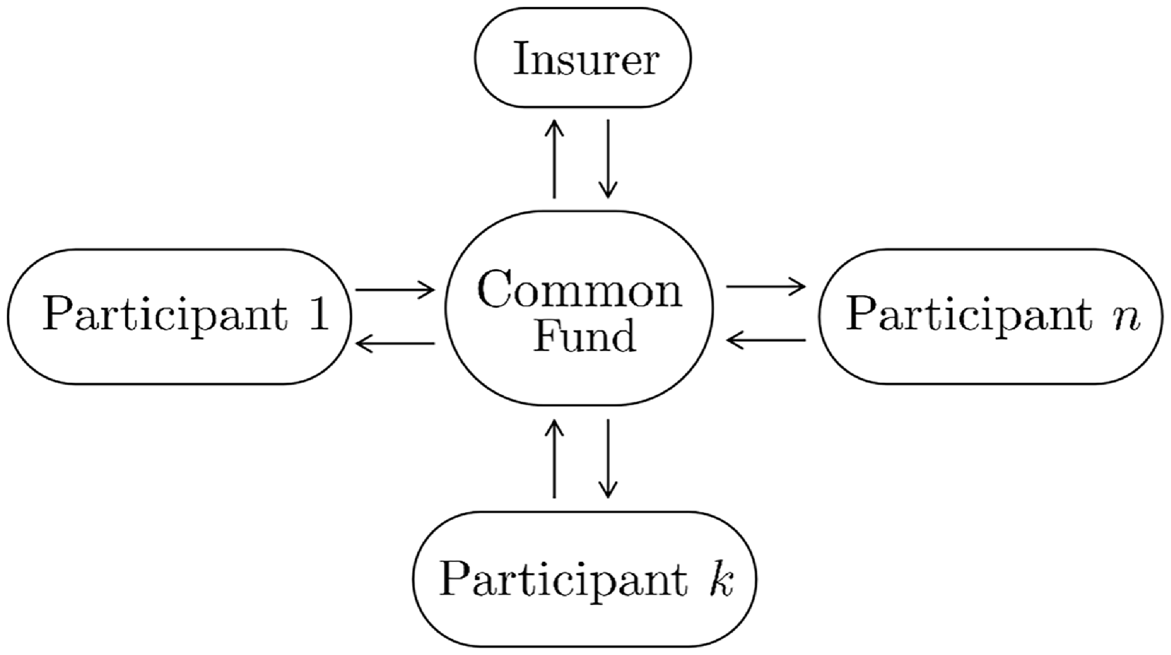
In the model of P2P insurance, participants’ risks are aggregated and separated into two layers. The first layer of small-to-medium losses is retained within a common fund, and the second layer of severe losses is covered by an insurer. Specifically, at the start of the insurance period, all the participants contribute to a common fund by depositing D. At the end of the insurance period, the participants’ losses are first covered by the common fund, with the insurer stepping in for any excess losses. Moreover, any remaining balance in the common fund is refunded to all participants (see Figure 1 for an illustration).

Figure 1.

Overview of the framework of P2P insurance.

Under this arrangement, the insurer assumes liability for losses exceeding the deposit, that is, for $X-D$ . The common fund’s risk-sharing responsibility is capped at D, ensuring limited liability for participants. Thus, the common fund must purchase insurance coverage with a deductible equal to the deposit D. In setting the premium, the insurer adds a risk loading $\theta\gt0$ to the fair premium. Consequently, the total premiumFootnote ² is

(2.1) \begin{equation}\Pi= (1+\theta)\mathbb{E}[(X-D)_{+}].\end{equation}

In the next section, we will decompose the costs involved in P2P insurance according to its underlying risk-sharing arrangement.

Figure 2.

Decomposition of the cost in P2P insurance.

2.3. Fixed and variable costs

In P2P insurance, the entire group initially contributes a total amount of $\Pi + D$ . The deposit D corresponds to the deductible, representing the portion of risk retained by the community. Due to the presence of a refund mechanism and the absence of risk loading, risk sharing within the common fund is typically more economical than the insurer’s underwriting costs. However, the cost for risk sharing is variable, as it depends on the actual loss outcomes. In contrast, the insurer’s underwriting cost $ \Pi $ is nonrefundable, generally higher, and predetermined.

We now provide a mathematical decomposition of the cost structure in P2P insurance. Let $\pi_{k}$ and $d_{k}$ for $k=1,\ldots,n$ represent the portion of $\Pi$ and D contributed by each participant, respectively. Thus, we have $D=\sum_{k=1}^{n}d_{k}$ and $\Pi=\sum_{k=1}^{n}\pi_{k}$ . For simplicity of notation, we define

\[\alpha_k=\frac{\pi_k}{\Pi},\ \ \text{and}\ \ \beta_k=\frac{d_k}{D}.\]

By the summation condition, it follows that $\sum_{k=1}^n \alpha_k=1$ and $\sum_{k=1}^n\beta_k=1$ . Here, $\alpha_k$ represents the ratio of the premium contributed by participant k to the total premium $\Pi$ , and $\beta_k$ represents the ratio of the deposit contributed to the total deposit D, reflecting their share of the remaining deposit in the common fund.

At time 0, participant k contributes $\pi_{k}+ d_{k}$ , or equivalently $\alpha_k\Pi+\beta_kD$ , to the pool. At time 1, the participant receive a partial refund $\beta_k(D-X)_{+}$ from the common fund, where $z_+=\max\{z,0\}$ . Under this decomposition, the cost allocation for each participant consists of a fixed premium and a variable deposit. The premium contribution, $\pi_k=\alpha_k \Pi$ , is nonrefundable and fixed, whereas the deposit contribution, $d_k=\beta_k D$ , is refundable depending on the ultimate loss outcome within the common fund. Using the notation of $\alpha_k$ and $\beta_k$ , the cost for participant k in the P2P insurance is given by:

(2.2) \begin{equation} C_k=\alpha_k\Pi+\beta_kD-\beta_k(D-X)_+.\end{equation}

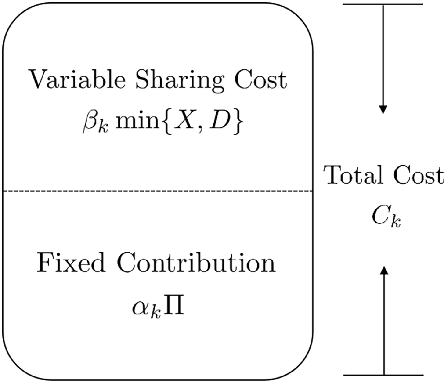
To summarize, the costs of P2P insurance consist of two parts (see Figure 2): (1) the fixed contribution, covering the group insurance premium paid to the insurer, and (2) the variable sharing cost, arising from the variability in the risk-sharing component managed by the common fund. This decomposition offers a flexible framework for adjusting each participant’s share of both the premium and deposit according to their risk profile and risk aversion, thereby enabling a reasonable approach for risk sharing within the group.

2.4. Actuarial fairness

In this section, we investigate actuarial fairness within the P2P insurance framework. Given participant heterogeneity, actuarial fairness is crucial for effectively pooling diverse risk types.

We begin with the expected cost for all participants in the P2P insurance model. Based on the participant’s cost in Equation (2.2), we have

\begin{align*} \sum_{k=1}^n C_k = (1+\theta)\mathbb{E}[(X-D)_{+}]+\min \left\{D,X \right\}.\end{align*}

Using this result, the expected total cost of all participants is given by:

(2.3) \begin{equation} \mathbb{E}\left[\sum_{k=1}^n C_k\right] = \mathbb{E}[X]+\Delta,\end{equation}

where $\Delta=\theta \mathbb{E}\left[(X-D)_{+}\right]$ . Equation (2.3) shows that the sum of the participants’ expected costs exceeds their expected income, with the additional cost component $\Delta$ arising from the insurer’s risk loading.

To obtain actuarial fairness among peers, we decompose both $\mathbb{E}[X]$ and $\Delta$ among all participants. We decompose each participant’s expected cost $\mathbb{E}[C_k]$ as his/her expected loss $\mathbb{E}[X_k]$ and an additional extra cost $\Delta_k$ . We have

(2.4) \begin{equation} \mathbb{E}[C_k]=\mathbb{E}[X_k]+\Delta_k,\end{equation}

where $\sum_{k=1}^{n} \Delta_k=\Delta$ . We define $\rho_k = \frac{\Delta_k}{\Delta}$ as the proportion of the total additional costs paid by participant k, and we can obtain $\sum_{k=1}^{n} \rho_k = 1$ . Substituting Equation (2.2) into Equation (2.4) yields:

(2.5) \begin{equation} \mathbb{E}\left[\min \left\{D,X \right\}\right]\beta_k=\mathbb{E}[X_k]+\rho_k\theta\mathbb{E}[(X-D)_{+}]-\alpha_k(1+\theta)\mathbb{E}[(X-D)_{+}],\end{equation}

which establishes the specified relationship between $\alpha_k$ and $\beta_k$ . It is straightforward to verify the summation condition $\sum_{k=1}^{n}\beta_{k}=1$ holds naturally if $\sum_{k=1}^n \alpha_k=1$ .

Remark 1. The fairness condition (2.4) requires that participants contribute an additional expected cost $\Delta_k$ on top of their own expected loss $\mathbb{E}[X_k]$ . This differs from the traditional definition of actuarial fairness in the literature, where the additional costs incurred from external insurance are not considered, that is,

\[\mathbb{E}[\tilde{C}_k] = \mathbb{E}[X_k],\]

where

\[\tilde{C}_k = \alpha_k \mathbb{E}[(X-D)_{+}]+\beta_k \min(D,X).\]

Our consideration of $\rho_k$ stems from the fact that the additional cost $\Delta$ , arising from risk loading $\theta$ , are additional expenses borne by the policyholders. In the P2P framework, where all participants are treated equally, it is essential to ensure fairness among all participants. Particularly under heterogeneous conditions, individuals with different risk characteristics contribute differently to the aggregate risk, meaning that each participant contributes a different proportion of the extra costs. Therefore, when examining actuarial fairness within the current framework, it is essential to account for the impact of these additional costs. Moreover, the classical condition for actuarial fairness in risk sharing (e.g., see Abdikerimova and Feng, Reference Abdikerimova and Feng2022) emerges as a special case of our proposed formulation when $\Delta_k = 0$ .

In addition, when $ D = 0 $ , the P2P insurance model reduces to traditional insurance. In this case, there is no variable cost, and the parameter $ \beta_k $ becomes irrelevant. The allocation parameter $ \alpha_k $ simplifies to:

\[\alpha_k = \frac{\mathbb{E}[X_k] + \rho_k \theta \mathbb{E}[X]}{(1 + \theta)\mathbb{E}[X]},\]

which represents the distribution of the total premium among participants. Conversely, when $ D = M $ , participants fully share all losses, rendering $ \alpha_k $ irrelevant. In this scenario, $ \beta_k $ is given by:

\[\beta_k = \frac{\mathbb{E}[X_k]}{\mathbb{E}[X]}.\]

These two extreme cases illustrate that it is meaningful to consider both $ \alpha_k $ and $ \beta_k $ simultaneously only when $ D \in (0, M) $ . Under this condition, the relationship between $ \alpha_k $ and $ \beta_k $ is characterized by the derivative:

\[\frac{\mathrm{d} \beta_k(\alpha_k)}{\mathrm{d} \alpha_k} = -\frac{(1+\theta)\mathbb{E}[(X - D)_+]}{\mathbb{E}[\!\min\{D, X\}]} \lt 0.\]

This implies a substitution effect: as participant k increases their premium share $ \alpha_k $ , they can reduce their required deposit $ \beta_k $ . This trade-off aligns with intuitive expectations, as each participant aims to balance their contributions to the nonrefundable premium pool $ \Pi $ and the potentially refundable deposit D.

2.5. Optimization problem for central planner

In this study, we adopt a mean-variance framework, where the utility for participant k is given by $\mathbb{E}[W_k]-\gamma_k \operatorname{Var}[W_k]$ , with $\gamma_k\gt0$ and $W_k$ is participant k’s wealth at time 1. In the mean-variance framework, any deterministic initial wealth is irrelevant and is therefore normalized to 0. Thus, $W_k$ can be expressed as:

\[W_k=-C_k=-\alpha_k (1+\theta)\mathbb{E}[(X - D)_+]-\beta_kD+\beta_k(D-X)_+ .\]

Suppose there exists a central planner whose objective is to maximize the collective mean-variance utility of all participants. As discussed earlier, adjusting the $(\alpha_k, \beta_k)$ allows for individual-level trade-offs between cost efficiency and variability, and further varying the deposit D enables this trade-off to be made at the aggregate level across all participants. Therefore, the central planner’s decision variables are the risk-sharing rules $(\alpha_k, \beta_k)$ and the deposit level D. Thus, the central planner’s optimization problem can be defined as follows:

\[\max_{\substack{\{\alpha_1, \ldots, \alpha_n\} \in \mathbb{R}^n \\\{\beta_1, \ldots, \beta_n\} \in \mathbb{R}^n \\D \in (0, M)}} \sum_{k=1}^{n} \left( \mathbb{E}[W_k] - \gamma_k \operatorname{Var}[W_k] \right)\! .\]

We solve this optimization problem through a step-by-step approach as follows:

Step 1. Solve $(\alpha_k^*,\beta_k^*)$ for a given D, which we refer to as the optimal risk-sharing rule;

Step 2. Solve the optimal deposit $D^*\in (0, M)$ , based on the results in Step 1.

In this way, we eventually determine the optimal parameters $(\alpha_1^*,\ldots,\alpha_n^*,\beta_1^*,\ldots,\beta_n^*,D^*)$ .

In this paper, we analyze the optimization problem under two different scenarios: without individual rationality (IR) constraints, and with IR constraints. The IR constraint, which asserts that participation in the insurance should not be worse than maintaining individual risk, is often a foundational assumption in the optimal design of commercial insurance. In Section 3, we first derive the general optimal solution under the assumption that all participants are either willing or required to join the P2P insurance plan, thus disregarding the IR constraint. Subsequently, in Section 4, we introduce the IR constraint and characterize the resulting optimal solution.

3.1. Optimal risk-sharing rules

First, we consider optimizing $\alpha_k$ and $\beta_k$ for a given D. The corresponding optimization problem for Step 1 is:

Problem 1.

(3.1) \begin{align} & \max_{\substack{\{\alpha_1, \ldots, \alpha_n\} \in \mathbb{R}^n \\\{\beta_1, \ldots, \beta_n\} \in \mathbb{R}^n}} \sum_{k=1}^{n} \left( \mathbb{E}[W_k] - \gamma_k \, \operatorname{Var}[W_k] \right)\! ,\end{align}

(3.2) \begin{align}s.t.\quad & \sum_{k=1}^n \alpha_k=1,\ \ \sum_{k=1}^{n}\beta_{k}=1,\end{align}

(3.3) \begin{align} & \mathbb{E}[X_k]+\rho_k\theta\mathbb{E}[(X-D)_{+}]-\alpha_k(1+\theta)\mathbb{E}[(X-D)_{+}] \notag \\[3pt] &\quad =\mathbb{E}\left[\min \left\{D,X \right\}\right]\beta_k, \ \ \forall k \in \{1,\ldots,n\}.\end{align}

Solving Problem 1 yields the optimal solutions $\alpha_k^{*}$ and $\beta_k^{*}$ , which are characterized as follows.

Theorem 1. For a given D, the solution of Problem 1 is given by:

(3.4) \begin{align} \alpha_k^{*} & = \frac{\mathbb{E}\left[X_k\right] + \rho_k \theta \mathbb{E}[(X-D)_{+}] - \beta_k^{*}\mathbb{E}\left[\min \left\{D,X \right\}\right] }{(1+\theta)\mathbb{E}[(X-D)_{+}]},\end{align}

(3.5) \begin{align}\beta_k^{*} & =\frac{1}{\gamma_k\sum_{l=1}^n\frac{1}{\gamma_{l}}}.\end{align}

For the central planner, once the deposit D is determined, Theorem 1 provides the optimal allocation rule. It can be readily verified that the optimal $\beta_k^*$ is always constrained within the interval (0, 1). In contrast, no such constraint applies to $\alpha_k^*$ and the only requirements is that $\sum_{k=1}^n \alpha_k^*=1$ .

Remark 3. For the k-th participant, we have $\alpha_k^* \lt0$ if

\[\mathbb{E}\left[X_k\right] + \rho_k \theta\mathbb{E}[(X - D)_+] \lt \mathbb{E}\left[\beta_k^{*} \min \left\{D,X \right\}\right].\]

The condition suggests that $\alpha_k^* \lt 0$ may arise either when the participants bear a low $\rho_k$ , indicating they bear a small share of the additional cost, or when the participants have a large $\beta_k^*$ , meaning they assume the excessive uncertain costs. Interestingly, when $\alpha_k^* \lt 0$ , the participant may initially receive a payment from the common fund, rather than contributing to it. This situation, particularly when driven by a high $\beta_k^*$ , implies that the participant requires compensation for shouldering a larger share of risk.

The above facts reflect an interesting feature of P2P insurance that is different from traditional insurance: participants can take on the roles of both insurance ‘buyer’ and ‘seller’:

1. (1) As the ‘buyer’ type, characterized by $(\alpha_k^{*} \gt 0, \beta_k^{*} \gt 0)$ , the participant pays a positive fixed cost, $\alpha_k^{*}\Pi$ , and contributes $\beta_k^{*}D$ to cover variable costs.

2. (2) As the ‘seller’ type, characterized by $(\alpha_k^{*} \lt 0, \beta_k^{*} \gt 0)$ , the participant receives an income cash inflow of $-\alpha_k^{*}\Pi$ but is required to deposit $\beta_k^{*}D$ into the common fund to cover variable costs.

Now, we examine the effect of parameters related to $\alpha_k^{*}$ and $\beta_k^{*}$ . We begin by examining the effects of $\gamma_k$ and $\gamma_\ell \text{ for }\ell\neq k,$ on $\alpha_k^{*}$ and $\beta_k^{*}$ in the following corollary.

Corollary 1 shows that, an increase in the degree of risk aversion $\gamma_k$ leads to an increase in the participant’s optimal fixed premium payment ratio $\alpha_k^{*}$ and a corresponding decrease in the optimal deposit ratio $\beta_k^{*}$ . This outcome supports the idea that higher levels of risk aversion correlate with a preference for fixed cost structures.

Remark 4. Considering a heterogeneous case where $n = 2$ , we have:

\[\frac{1}{\beta_1^{*}} = 1 + \frac{\gamma_1}{\gamma_2}, \quad \frac{1}{\beta_2^{*}} = 1 + \frac{\gamma_2}{\gamma_1}.\]

It is straightforward to verify that $\beta_1^{*} \lt \beta_2^{*}$ if $\gamma_1 \gt \gamma_2$ , and vice versa. This example highlights the impact of risk aversion on $\beta_k^{*}$ : participants with higher risk aversion contribute a smaller share. We extend this analysis by introducing two types of participants, high-risk and low-risk, denoted by $X_H$ and $X_L$ , respectively. Let $n_H$ and $n_L$ denote the number of high-risk and low-risk participants. In this case, the optimal deposit ratios are given by:

\[\frac{1}{\beta_H^*} = n_H + n_L \frac{\gamma_H}{\gamma_L}, \quad \frac{1}{\beta_L^*} = n_L + n_H \frac{\gamma_L}{\gamma_H}.\]

Corollary 2 states that $ \alpha_k^{*} $ decreases with $ \theta $ when $ \rho_k $ is below the threshold $ \alpha_k^{*} $ . This implies that the peers are required to contribute a smaller share of the premium. Once $ \rho_k $ exceeds this threshold, $ \alpha_k^{*} $ increases with $ \theta $ , reflecting a greater required contribution.

This corollary shows that $\alpha_k^{*}$ increases with D when the deposit ratio $\beta_k^{*}$ lower than their proportional risk exposure in the entire pool and decreases otherwise. This conclusion aligns with the fairness condition, as it suggests that a group should contribute a larger share to the fixed premium when its deposit ratio is relatively lower, thus balancing the overall contributions within the pool.

Remark 5. We consider a special case where $n=2$ . Suppose $\mathbb{E}\left[X_2\right]=a\mathbb{E}\left[X_1\right]$ , and $\gamma_2 = b \gamma_1$ . Then, if $a=1$ and $b\gt1$ , we get

\begin{align*}\beta_1^* = \frac{1}{1+\frac{\gamma_1}{\gamma_2}} = \frac{1}{1+\frac{1}{b}} \gt \frac{1}{2} = \frac{\mathbb{E}\left[X_1\right]}{\mathbb{E}\left[X\right]},\quad \beta_2^* = \frac{1}{1+\frac{\gamma_2}{\gamma_1}} = \frac{1}{1+b} \lt \frac{1}{2} = \frac{\mathbb{E}\left[X_2\right]}{\mathbb{E}\left[X\right]}.\end{align*}

In this case, $\alpha_1^{*}$ decreases with D and $\alpha_2^{*}$ increases with D. If $a\gt1$ and $b=1$ , then

\begin{align*}\beta_1^* = \frac{1}{1+\frac{\gamma_1}{\gamma_2}} = \frac{1}{2 } \gt \frac{1}{1+a} = \frac{\mathbb{E}\left[X_1\right]}{\mathbb{E}\left[X\right]},\quad \beta_2^* = \frac{1}{1+\frac{\gamma_2}{\gamma_1} } = \frac{1}{2 } \lt \frac{1}{ 1+\frac{1}{a}} = \frac{\mathbb{E}\left[X_2\right]}{\mathbb{E}\left[X\right]}.\end{align*}

In this case, $\alpha_1^{*}$ decreases with D and $\alpha_2^{*}$ increases with D.

3.2. Optimal deposit

So far, we have solved $(\alpha_k^{*},\beta_k^{*})$ for any given D. Building on this analysis, we now proceed to determine the optimal deposit. The problem for Step 2 is formulated as follows:

Problem 2.

(3.6) \begin{align} & \max\limits_{D \in (0,M)}\sum\limits_{k=1}^{n}\left(\mathbb{E}[W_k]-\gamma_k \operatorname{Var}[W_k]\right).\end{align}

Based on Theorem 1, we derive the following theorem.

Theorem 2. The optimal deposit $ D^* $ for Problem 1 is characterized as follows: If

\[\theta \lt \frac{2}{\sum_{k=1}^n\frac{1}{\gamma_k}} \left(M - \mathbb{E}[X] \right),\]

then $ D^* $ is the unique solution to the equation:

(3.7) \begin{equation}\frac{\theta}{2} \sum_{k=1}^n\frac{1}{\gamma_k} = \int_0^{D^*} F_X(s) \, \mathrm{d}s.\end{equation}

Theorem 2 indicates that participants prefer to combine risk sharing with traditional insurance coverage when the risk loading factor $\theta$ is below a certain threshold. In contrast, when the insurance price is excessively high, the proof of Theorem 2 demonstrates that the objective function is increasing in D. This implies that participants are inclined to maximize their risk sharing within the common fund rather than relying on traditional insurance.

4.1. Optimal risk-sharing rules with IR constraints

Given $\rho_1, \ldots, \rho_n$ and D, we have the following Step 1 optimization problem:

Problem 3.

(4.3) \begin{align} & \max_{\substack{\{\alpha_1, \ldots, \alpha_n\} \in \mathbb{R}^n \\\{\beta_1, \ldots, \beta_n\} \in \mathbb{R}^n}} \sum\limits_{k=1}^{n}\left(\mathbb{E}[W_k]-\gamma_k \operatorname{Var}[W_k]\right),\end{align}

(4.4) \begin{align} s.t.\quad & \sum_{k=1}^n \alpha_k=1,\quad \sum_{k=1}^{n}\beta_{k}=1,\end{align}

(4.5) \begin{align} & \rho_k \leq \frac{\gamma_k\operatorname{Var}[X_k]-\gamma_k\beta_k^2\operatorname{Var}[\! \min\{X,D\}]}{\theta \mathbb{E}[(X-D)_{+}]}, \ \ \forall k \in \{1,\ldots,n\},\end{align}

(4.6) \begin{align} & \mathbb{E}[X_k]+\rho_k\theta\mathbb{E}[(X-D)_{+}]-\alpha_k(1+\theta)\mathbb{E}[(X-D)_{+}] \notag \\ &=\mathbb{E}\left[\min \left\{D,X \right\}\right]\beta_k, \ \ \forall k \in \{1,\ldots,n\}.\end{align}

By solving Problem 3, we obtain the following results of $\alpha_k^{*}$ and $\beta_k^{*}$ .

Theorem 3. Given $\rho_1, \ldots, \rho_n$ and D, if $\rho_k \leq \frac{\gamma_k\operatorname{Var}[X_k]}{\theta \mathbb{E}[(X-D)_{+}]}$ for any k, then no solution for Problem 3 exists. Otherwise, denote $\mathcal{J}$ be the set of all k satisfying:

(4.7) \begin{equation}\rho_k \gt\frac{\gamma_k\operatorname{Var}[X_k]-\frac{1}{\gamma_k(\sum_{k=1}^n\frac{1}{\gamma_k})^2}\operatorname{Var}[\! \min\{X,D\}]}{\theta \mathbb{E}[(X-D)_{+}]},\end{equation}

and $\mathcal{K}$ is given by $\mathcal{K} = \{1, \ldots, n\} \setminus \mathcal{J}$ . Then,

1. (1) If $\mathcal{K}$ is nonempty, and for all $k \in \mathcal{K}$ ,

   (4.8) \begin{equation}\rho_k \leq \frac{\gamma_k\operatorname{Var}[X_k]-\frac{\left(1-\sum_{k \in \mathcal{J}}\sqrt{\frac{\gamma_k\operatorname{Var}[X_k]-\rho_k\theta \mathbb{E}[(X-D)_{+}]}{\gamma_k\operatorname{Var}[\! \min\{X,D\}]}}\right)^2}{\gamma_k\left(\sum_{k \in \mathcal{K}}\frac{1}{\gamma_{k}}\right)^2}\operatorname{Var}[\! \min\{X,D\}]}{\theta \mathbb{E}[(X-D)_{+}]},\end{equation}
   then the solution for Problem 3 is given by:
   (4.9) \begin{align} &\alpha_k^{*} = \frac{\mathbb{E}\left[X_k\right] + \rho_k \theta \mathbb{E}[(X-D)_{+}] - \beta_k^{*}\mathbb{E}\left[\min \left\{D,X \right\}\right] }{(1+\theta)\mathbb{E}[(X-D)_{+}]},\end{align}
   (4.10) \begin{align} &\beta_k^{*} =\frac{1-\sum_{k \in \mathcal{J}}\beta_k^*}{\gamma_k\sum_{k \in \mathcal{K}}\frac{1}{\gamma_{k}}}, k \in \mathcal{K},\end{align}
   (4.11) \begin{align} & \beta_k^{*} = \sqrt{\frac{\gamma_k\operatorname{Var}[X_k]-\rho_k\theta \mathbb{E}[(X-D)_{+}]}{\gamma_k\operatorname{Var}[\! \min\{X,D\}]}}, k \in \mathcal{J},\end{align}

   where we note that if $\mathcal{J}$ is empty, then $\sum_{k \in \mathcal{J}}\beta_k^*=0$ .

2. (2) Otherwise, no solution exists for Problem 3.

For the central planner, once $\rho_k$ and D are specified, Theorem 3 determines the optimal risk-sharing rule. When both $\mathcal{J}$ and $\mathcal{K}$ are nonempty, we observe the following distinct patterns: (1) for participants $ k \in \mathcal{J} $ , $ \beta_k^* $ decreases with respect to $ \rho_k $ . This inverse relationship indicates that the more additional cost a participant is allocated, the smaller the random cost they should bear. (2) For participants in $ k \in \mathcal{K} $ , $ \beta_k^* $ remains independent of their corresponding $ \rho_k $ , demonstrating complete independence between these variables.

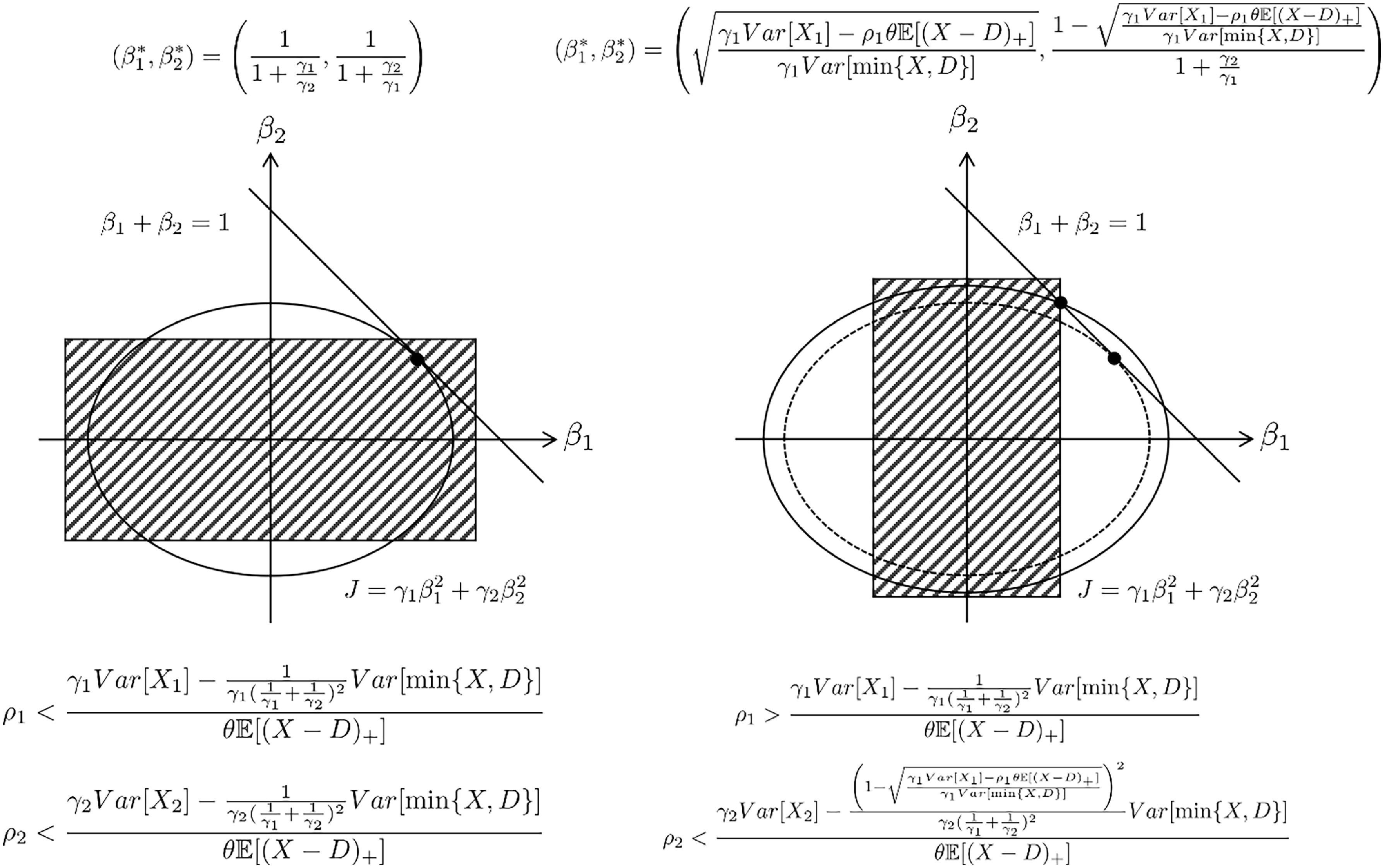
Remark 8. We illustrate the results of Theorem 3 using a simple example where $ n = 2 $ . As depicted in Figure 3, the objective function forms an ellipse. The feasible solutions for $ (\beta_1, \beta_2) $ lie at the intersections of the ellipse and the constraint $ \beta_1 + \beta_2 = 1 $ . The left panel of Figure 3 illustrates the case where $\mathcal{J}$ is empty. Here, the unconstrained minimum of the ellipse lies within the feasible region. The parameters $ (\beta_1^*, \beta_2^*) $ are given by: $\beta_1^* = \frac{1}{1 + \frac{\gamma_1}{\gamma_2}}$ and $\beta_2^* = \frac{1}{1 + \frac{\gamma_2}{\gamma_1}}$ .

Figure 3.

Schematic illustration of Theorem 3.

The right panel of Figure 3 depicts the case where both $\mathcal{J}$ and $\mathcal{K}$ are nonempty. In this case, the feasible region for $ \beta_1 $ excludes the unconstrained minimizer. As a result, $ \beta_1^* $ lies on the boundary. Although the feasible region for $ \beta_2 $ includes the unconstrained minimizer, the constraint $ \beta_2^* = 1 - \beta_1^* $ forces $ \beta_2^* $ to exceed $ \frac{1}{1 + \frac{\gamma_2}{\gamma_1}} $ because $ \beta_1^* $ is below its unconstrained optimum.

4.2. Optimal deposit with IR constraints

4.2.1. Characterization of feasible region

Before we derive the optimal deposit $D^*$ , we first characterize the feasible region $\mathcal{D}$ under IR constraints in this section.

As established in Theorem 3, when both $ \mathcal{K} $ and $ \mathcal{J} $ are nonempty, the index set pair $(\mathcal{K}, \mathcal{J})$ admits a total of $2^n - 2$ configurations. Including the special case where $ \mathcal{J} $ is empty, the total number of configurations becomes $2^n - 1$ . Each configuration corresponds to a (possibly overlapping) subinterval of the deposit domain (0, M), within which the solution $(\alpha^*_k, \beta^*_k)$ exists. Given the parameters $\rho_1, \ldots, \rho_n$ , let

\[\mathcal{D} = \bigcup_{t=1}^{2^n - 1} \mathcal{D}_t\]

denote the feasible region for deposits, where $ \mathcal{D}_t $ denote the subinterval associated with the t -th configuration. Before proceeding with the analysis, we distinguish between two cases in Theorem 3:

• • When $\mathcal{J}$ is empty: if $\rho_k$ satisfies the following condition:

  (4.12) \begin{equation} \rho_k \leq \frac{\gamma_k\operatorname{Var}[X_k]-\frac{1}{\gamma_k\left(\sum_{k=1}^n\frac{1}{\gamma_k}\right)^2}\operatorname{Var}[\! \min\{X,D\}]}{\theta \mathbb{E}[(X-D)_{+}]}, \ \forall k \in \{1,\ldots ,n\}, \end{equation}
  then Problem 3 reduces to the unconstrained formulation in Problem 1. In this case, the solution $(\alpha^*_k, \beta^*_k)$ coincides with that in Theorem 1, where $\beta^*_k$ depends only on risk aversion and is independent of D, as shown in Equation (3.5).

• • When $\mathcal{J}$ is nonempty: if instead

  (4.13) \begin{equation}\frac{\gamma_k\operatorname{Var}[X_k]-\frac{1}{\gamma_k\left(\sum_{k=1}^n\frac{1}{\gamma_k}\right)^2}\operatorname{Var}[\! \min\{X,D\}]}{\theta \mathbb{E}[(X-D)_{+}]} \lt \rho_k \leq \frac{\gamma_k\operatorname{Var}[X_k]}{\theta \mathbb{E}[(X-D)_{+}]}, \ \forall k \in \mathcal{J},\end{equation}
  and for all $k \in \mathcal{K}$ , $\rho_k$ satisfy (4.8), then each $\beta^*_k$ is determined at the boundary of constraint (4.5). As shown in Equations (4.10) and (4.11), $\beta^*_k$ becomes a function of D.

This distinction is essential, as the relationship between $\beta^*$ and D fundamentally differs between the two cases. For convenience, we label the subinterval corresponding to inequality (4.12) as $\mathcal{D}_1$ , and those corresponding to inequality (4.13) as $\mathcal{D}_t$ , where $t \in \{2, \ldots, 2^n - 1\}$ .

In the following sections, we examine the structure of each subinterval $\mathcal{D}_t$ and then determine the existence and uniqueness of a local optimum $ D^*_t $ , and the closed-form expression for $ D^*_t $ when it exists. Specifically, in Sections 4.2.2 and 4.2.3, we introduce the local optimal $D^*_1$ within $\mathcal{D}_1$ and $\mathcal{D}_t$ for $t \in \{2, \ldots, 2^n - 1\}$ , respectively. Finally, the global optimal deposit $ D^* $ over the entire feasible region $ \mathcal{D} $ is determined as the one among these $ D^*_t $ that yields the highest objective function value.

4.2.2. Local optimal $D^*_1$ within $\mathcal{D}_1$

In this section, we start from $\mathcal{D}_1$ where inequality (4.12) holds. For simplicity, we define two tool functions as:

\begin{align*}\phi_k(D) & = \dfrac{\gamma_k \operatorname{Var}[X_k] - \frac{1}{\gamma_k \left( \sum_{k=1}^n \frac{1}{\gamma_k} \right)^2} \operatorname{Var}[\! \min\{X, D\}]}{\theta \, \mathbb{E}[(X - D)_{+}]}, \\[4pt]\psi_k(D) & = - \frac{2(D - \mathbb{E}[\!\min\{X, D\}])\mathbb{E}[(X - D)_{+}]+\operatorname{Var}[\! \min\{X, D\}]}{\gamma_k^2 \left( \sum_{k=1}^n \frac{1}{\gamma_k} \right)^2} + \operatorname{Var}[X_k].\end{align*}

Then, we characterize the structure of $\mathcal{D}_1$ through the following lemma:

Lemma 1. Given $\rho_1, \dots, \rho_n$ , the interval $\mathcal{D}_1$ is given by:

\[\mathcal{D}_1 = \bigcap_{k=1}^n \tilde{\mathcal{D}}_k,\]

where each $\tilde{\mathcal{D}}_k$ is determined according to the following cases:

1. (1) When

   \[\operatorname{Var}[X_k] - \frac{ \operatorname{Var}[X]}{\gamma_k^2 \left( \sum_{j=1}^n \frac{1}{\gamma_j} \right)^2} \geq 0, \]

   1. (a) If $\rho_k \gt \frac{\gamma_k \operatorname{Var}[X_k]}{\theta \, \mathbb{E}[X]}$ , there exists a unique $\hat{D}_k$ such that $\phi_k(\hat{D}_k) = \rho_k$ , and we have $\tilde{\mathcal{D}}_k = [\hat{D}_k, M)$ ;

   2. (b) If $\rho_k \leq \frac{\gamma_k \operatorname{Var}[X_k]}{\theta \, \mathbb{E}[X]}$ , we have $\tilde{\mathcal{D}}_k = (0, M)$ .

2. (2) When

   \[ \operatorname{Var}[X_k] - \frac{\operatorname{Var}[X]}{\gamma_k^2 \left( \sum_{j=1}^n \frac{1}{\gamma_j} \right)^2} \lt 0, \]
   then there exists a unique $\tilde{D}_k$ such that $\psi_k(\tilde{D}_k) = 0$ . Then,

   1. (a) If $\rho_k \gt \phi_k(\tilde{D}_k)$ , we have $\tilde{\mathcal{D}}_k = \emptyset$ ;

   2. (b) If $\frac{\gamma_k \operatorname{Var}[X_k]}{\theta \, \mathbb{E}[X]} \lt \rho_k \leq \phi_k(\tilde{D}_k)$ , there exist $\underline{\hat{D}}_k \leq \hat{\overline{D}}_k$ such that $\phi_k(\underline{\hat{D}}_k) = \phi_k(\hat{\overline{D}}_k) = \rho_k$ , and we have $\tilde{\mathcal{D}}_k = [\underline{\hat{D}}_k, \hat{\overline{D}}_k]$ ;

   3. (c) If $\rho_k \leq \frac{\gamma_k \operatorname{Var}[X_k]}{\theta \, \mathbb{E}[X]}$ , we have $\tilde{\mathcal{D}}_k = (0, \hat{D}_k]$ .

In what follows, we identify the associated local optimal deposit $ D^*_1 $ within $ \mathcal{D}_1 $ , if it exists. Note that, for given $ \rho_1, \ldots, \rho_n $ , $ \mathcal{D}_1 $ is possibly empty. To proceed with the analysis, we assume that $ \mathcal{D}_1 $ is a nonempty closed interval, ensuring the existence of a $ D^*_1 $ . Then we establish the following theorem.

Theorem 4. Assume that $ \mathcal{D}_1 $ is a nonempty closed interval, denoted by $ \mathcal{D}_1 = [\underline{D}_1, \overline{D}_1] $ . Given $\rho_1, \ldots, \rho_n$ , $ D^*_1 $ is given by:

1. (1) If

   \[\theta - \frac{2}{\sum_{k=1}^n\frac{1}{\gamma_k}} \int_0^{\underline{D}_1} F_X(s)\mathrm{d}s \leq 0,\]
   then $ D^*_1 = \underline{D}_1 $ .

2. (2) If

   \[\theta - \frac{2}{\sum_{k=1}^n\frac{1}{\gamma_k}} \int_0^{\overline{D}_1} F_X(s)\mathrm{d}s \geq 0,\]
   then $ D^*_1 = \overline{D}_1 $ .

3. (3) If

   \[\theta - \frac{2}{\sum_{k=1}^n\frac{1}{\gamma_k}} \int_0^{\underline{D}_1} F_X(s)\mathrm{d}s \gt 0, \ \text{and}\ \ \theta - \frac{2}{\sum_{k=1}^n\frac{1}{\gamma_k}} \int_0^{\overline{D}_1} F_X(s)\mathrm{d}s \lt 0,\]
   then $ D^*_1 $ is determined as follows:
   (4.14) \begin{equation} D^*_1 = \underline{D}_1 \cdot \mathbb{I} [D^o \lt \underline{D}_1] + D^o \cdot \mathbb{I}[\underline{D}_1 \leq D^o \leq \overline{D}_1] + \overline{D}_1 \cdot \mathbb{I} [D^o \gt \overline{D}_1], \end{equation}
   where $ D^o $ is the unique solution to the equation:
   (4.15) \begin{equation} \frac{\theta}{2} \sum_{k=1}^n\frac{1}{\gamma_k} = \int_0^{D^o} F_X(s) \, \mathrm{d}s. \end{equation}

4.2.3. Local optimal $D^*_t$ within $\mathcal{D}_t$ for $t \in \{2, \ldots, 2^n - 1\}$

We now turn to $ \mathcal{D}_t $ for $ t \in \{2, \dots, 2^n - 1\} $ where the inequality (4.13) holds. In what follows, we analyze the structure of $ \mathcal{D}_t $ for a given t. We denote the index sets corresponding to the k-th configuration as $ \mathcal{K}_t $ and $ \mathcal{J}_t $ , respectively. Similar to Lemma 1, we have

\[\mathcal{D}_t = \tilde{\mathcal{D}}_{\mathcal{J}_t} \bigcap \tilde{\mathcal{D}}_{\mathcal{K}_t},\]

where

\[\tilde{\mathcal{D}}_{\mathcal{K}_t} = \bigcap_{k \in \mathcal{K}_t} \tilde{\mathcal{D}}_k, \ \ \text{and} \ \ \tilde{\mathcal{D}}_{\mathcal{J}_t} = \bigcap_{k \in \mathcal{J}_t} \tilde{\mathcal{D}}_k.\]

We first discuss the structure of $\tilde{\mathcal{D}}_{\mathcal{J}_t}$ . For simplicity, we define a tool function as:

\[\tilde{\phi}_k(D) = \frac{\gamma_k\operatorname{Var}[X_k]}{\theta \mathbb{E}[(X-D)_{+}]},\]

and then have the following lemma:

Lemma 2. Given $\rho_1, \ldots, \rho_n$ , the interval $\tilde{\mathcal{D}}_{\mathcal{J}_t}$ can be expressed as:

\[\tilde{\mathcal{D}}_{\mathcal{J}_t} = \bigcap_{k \in \mathcal{J}_t} \tilde{\mathcal{D}}_k,\]

where each $\tilde{\mathcal{D}}_k$ is determined according to the following cases:

1. (1) When

   \[ \operatorname{Var}[X_k] - \frac{ \operatorname{Var}[X]}{\gamma_k^2 \left( \sum_{j=1}^n \frac{1}{\gamma_j} \right)^2} \geq 0, \]

   1. (a) If $\rho_k \gt \frac{\gamma_k \operatorname{Var}[X_k]}{\theta \, \mathbb{E}[X]}$ , there exists a unique $\hat{D}_k$ such that $\phi_k(\hat{D}_k) = \rho_k$ , and a unique $D^{\sharp}_k$ such that $\tilde{\phi}_k(D^{\sharp}_k) = \rho_k$ , and then we have $\tilde{\mathcal{D}}_k = [D^{\sharp}_k, \hat{D}_k]$ ;

   2. (b) If $\rho_k \leq \frac{\gamma_k \operatorname{Var}[X_k]}{\theta \, \mathbb{E}[X]}$ , we have $\tilde{\mathcal{D}}_k = \emptyset$ .

2. (2) When

   \[ \operatorname{Var}[X_k] - \frac{\operatorname{Var}[X]}{\gamma_k^2 \left( \sum_{j=1}^n \frac{1}{\gamma_j} \right)^2} \lt 0, \]
   then there exists a unique $\tilde{D}_k$ such that $\psi_k(\tilde{D}_k) = 0$ . Then,

   1. (a) If $\rho_k \gt \phi_k(\tilde{D}_k)$ , we have $\tilde{\mathcal{D}}_k = [D^{\sharp}_k, M)$ ;

   2. (b) If $\frac{\gamma_k \operatorname{Var}[X_k]}{\theta \, \mathbb{E}[X]} \lt \rho_k \leq \phi_k(\tilde{D}_k)$ , then there exist $\underline{\hat{D}}_k \leq \hat{\overline{D}}_k$ such that $\phi_k(\underline{\hat{D}}_k) = \phi_k( \hat{\overline{D}}_k ) = \rho_k$ , and we have $\tilde{\mathcal{D}}_k = [D^{\sharp}_k, \underline{\hat{D}}_k]$ , or $\tilde{\mathcal{D}}_k = [\underline{\hat{D}}_k, M)$ ;

   3. (c) If $\rho_k \leq \frac{\gamma_k \operatorname{Var}[X_k]}{\theta \, \mathbb{E}[X]}$ , we have $\tilde{\mathcal{D}}_k = [ \hat{D}_k, M)$ .

Notice that the constraints associated with $ \tilde{\mathcal{D}}_{\mathcal{K}_t} $ are inherently dependent on the structure of $ \tilde{\mathcal{D}}_{\mathcal{J}_t} $ . As shown in the proof of Theorem 3, the inequality (4.8) is meaningful only if the set $ \tilde{\mathcal{D}}_{\mathcal{J}_t} $ is nonempty. To ensure the validity of the analysis for $ \tilde{\mathcal{D}}_{\mathcal{K}_t}$ , $ \tilde{\mathcal{D}}_{\mathcal{J}_t} $ must be nonempty. Before delving into the structure of $\tilde{\mathcal{D}}_{\mathcal{K}_t}$ , we first introduce the following tool functions:

\begin{align*}& \kappa_k(D) = \left(1-\sum_{k \in \mathcal{J}}\sqrt{\frac{\gamma_k\operatorname{Var}[X_k]-\rho_k\theta \mathbb{E}[(X-D)_{+}]}{\gamma_k\operatorname{Var}[\! \min\{X,D\}]}}\right)^2 \operatorname{Var}[\! \min\{X,D\}],\\&\eta_k(D) = \frac{\gamma_k\operatorname{Var}[X_k]-\frac{\kappa_k(D)}{\gamma_k\left(\sum_{k \in \mathcal{K}}\frac{1}{\gamma_{k}}\right)^2} }{\theta \mathbb{E}[(X-D)_{+}]},\\&h(D) = -\frac{ \frac{\,\mathrm{d} \kappa_k(D)}{\,\mathrm{d} D} \mathbb{E}[(X-D)_{+}]}{\gamma_k\left(\sum_{k \in \mathcal{K}}\frac{1}{\gamma_{k}}\right)^2} + S_X(D)\left( \gamma_k\operatorname{Var}[X_k]-\frac{\kappa_k(D)}{\gamma_k\left(\sum_{k \in \mathcal{K}}\frac{1}{\gamma_{k}}\right)^2} \right)\kern-2.5pt.\end{align*}

Then, we can establish the following lemma:

Lemma 3. Assume that $ \tilde{\mathcal{D}}_{\mathcal{J}_t} $ is a nonempty closed interval, denoted by $ \tilde{\mathcal{D}}_{\mathcal{J}_t} = [\underline{D}_{\mathcal{J}_t}, \overline{D}_{\mathcal{J}_t}] $ . Given $\rho_1, \ldots, \rho_n$ , then $\tilde{\mathcal{D}}_{\mathcal{K}_t}$ can be expressed as:

\[\tilde{\mathcal{D}}_{\mathcal{K}_t} = \bigcap_{k \in \mathcal{K}_t} \tilde{\mathcal{D}}_k,\]

where each $\tilde{\mathcal{D}}_k$ is determined according to the following cases:

1. (1) When $h_k(\underline{D}_{\mathcal{J}_t}) \geq 0$ and $h_k(\overline{D}_{\mathcal{J}_t}) \geq 0$ , then:

   1. (a) If $\rho_k \gt \eta_k(\overline{D}_{\mathcal{J}_t})$ , we have $\tilde{\mathcal{D}}_k = \emptyset$ ;

   2. (b) If $\rho_k \lt \eta_k(\underline{D}_{\mathcal{J}_t})$ , we have $\tilde{\mathcal{D}}_k = [\underline{D}_{\mathcal{J}_t}, \overline{D}_{\mathcal{J}_t} ]$ ;

   3. (c) If $\eta_k(\underline{D}_{\mathcal{J}_t}) \leq \rho_k \leq \eta_k(\overline{D}_{\mathcal{J}_t})$ , there uniquely exists $D^{+}_k$ such that $\rho_k = \eta_k(D^{+}_k)$ , and we have $\tilde{\mathcal{D}}_k = [D^{+}_k, \overline{D}_{\mathcal{J}_t} ]$ .

2. (2) When $h_k(\underline{D}_{\mathcal{J}_t}) \leq 0$ and $h_k(\overline{D}_{\mathcal{J}_t}) \leq 0$ , then:

   1. (a) If $\rho_k \gt \eta_k(\underline{D}_{\mathcal{J}_t})$ , we have $\tilde{\mathcal{D}}_k = \emptyset$ ;

   2. (b) If $\rho_k \lt \eta_k(\overline{D}_{\mathcal{J}_t})$ , we have $\tilde{\mathcal{D}}_k = [\underline{D}_{\mathcal{J}_t}, \overline{D}_{\mathcal{J}_t} ]$ ;

   3. (c) If $\eta_k(\overline{D}_{\mathcal{J}_t}) \leq \rho_k \leq \eta_k(\underline{D}_{\mathcal{J}_t})$ , we have $\tilde{\mathcal{D}}_k = [\underline{D}_{\mathcal{J}_t},D^{+}_k ]$ .

3. (3) When $h_k(\underline{D}_{\mathcal{J}_t}) \gt 0$ and $h_k(\overline{D}_{\mathcal{J}_t}) \lt 0$ , there uniquely exists $D^{\eta}_k$ such that $h_k(D^{\eta}_k) = 0$ , then:

   1. (a) If $\rho_k \gt \eta_k(D^{\eta}_k)$ , we have $\tilde{\mathcal{D}}_k = \emptyset$ ;

   2. (b) If $\max\{\eta_k(\overline{D}_{\mathcal{J}_t}),\eta_k(\underline{D}_{\mathcal{J}_t})\} \leq \rho_k \leq \eta_k(D^{\eta}_k)$ , then there exist $\underline{D}^+_k \leq \overline{D}^+_k$ such that $\rho_k = \eta_k(\underline{D}^+_k) = \eta_k(\overline{D}^+_k)$ , and we have $\tilde{\mathcal{D}}_k = [\underline{D}_{\mathcal{J}_t}, \underline{D}^+_k]$ or $\tilde{\mathcal{D}}_k = [ \overline{D}^+_k, \overline{D}_{\mathcal{J}_t}]$ ;

   3. (c) If $\min\{\eta_k(\overline{D}_{\mathcal{J}_t}),\eta_k(\underline{D}_{\mathcal{J}_t})\} \leq \rho_k \lt \max\{\eta_k(\overline{D}_{\mathcal{J}_t}),\eta_k(\underline{D}_{\mathcal{J}_t})\}$ , then we have $\tilde{\mathcal{D}}_k = [\underline{D}_{\mathcal{J}_t}, D^+_k]$ if $\eta_k(\overline{D}_{\mathcal{J}_t}) \gt \eta_k(\underline{D}_{\mathcal{J}_t})$ , and $\tilde{\mathcal{D}}_k = [D^+_k, \overline{D}_{\mathcal{J}_t}]$ if $\eta_k(\overline{D}_{\mathcal{J}_t}) \lt \eta_k(\underline{D}_{\mathcal{J}_t})$ ;

   4. (d) If $\rho_k \lt \min\{\eta_k(\overline{D}_{\mathcal{J}_t}),\eta_k(\underline{D}_{\mathcal{J}_t})\}$ , we have $\tilde{\mathcal{D}}_k = \emptyset$ .

Having characterized each $\mathcal{D}_t$ for $t \in \{2, \ldots, 2^n - 1\}$ , we now identify the local optimal deposit $D^*_t$ , when it exists. Similar to the approach in Theorem 4, we assume that $\mathcal{D}_t$ is a nonempty closed interval, which guarantees the existence of a local optimum. We obtain the following result.

Theorem 5. Assume that $\mathcal{D}_t $ is a nonempty closed interval, denoted by $ \mathcal{D}_t = [\underline{D}_t, \overline{D}_t] $ . Given $\rho_1, \ldots, \rho_n$ , if there exist $D^o_t \in \mathcal{D}_t$ which is the solution to the following equation:

\begin{align*}\sum_{k \in \mathcal{K}_t}\rho_k \theta S_X(D) &= \frac{2}{\sum_{k \in \mathcal{K}_t} \frac{1}{\gamma_k}} \left(\sqrt{\operatorname{Var}[\! \min\{X,D\}]} - \sum_{k \in \mathcal{J}_t} \sqrt{\operatorname{Var}[X_k]- \frac{\rho_k}{\gamma_k}\theta \mathbb{E}[(X-D)_{+}] } \right) \\&\quad \cdot S_X(D) \left(\frac{D-\mathbb{E}[\!\min\{X,D\}]}{\sqrt{\operatorname{Var}[\! \min\{X,D\}]}}- \sum_{k \in \mathcal{J}_t} \frac{\frac{\rho_k}{\gamma_k}\theta}{2\sqrt{\operatorname{Var}[X_k]- \frac{\rho_k}{\gamma_k}\theta \mathbb{E}[(X-D)_{+}] }}\right),\end{align*}

then $D^*_t = D^o_t$ . Otherwise,

\[D^*_t = \arg \max_{D \in \{\underline{D}_t, \overline{D}_t \} } \sum\limits_{k=1}^{n}\left(\mathbb{E}[W_k]-\gamma_k \operatorname{Var}[W_k]\right).\]

4.2.4. Characterization of global optimal deposit $D^*$

In the previous sections, we have established that the global feasible region $ \mathcal{D} $ is the union of $ 2^n - 1 $ subfeasible regions $ \mathcal{D}_t $ , each corresponding to a configuration of the index sets $ (\mathcal{K}, \mathcal{J}) $ . We also examined each $ \mathcal{D}_t $ individually and identify the associated local optimal deposit $ D^*_t $ , if it exists.

Once all potentially valid local optima $ D^*_t $ are obtained, the global optimal deposit $ D^* $ is identified as the one maximizing the objective function. Specifically, $D^*=D^*_{t^*}$ with

(4.16) \begin{equation} t^* = \arg\max_{t \in \mathcal{T}} \sum_{k=1}^{n} \left( \mathbb{E}[W_k(D^*_t)] - \gamma_k \operatorname{Var} [W_k(D^*_t)] \right),\end{equation}

and

\begin{equation}\mathcal{T} = \left\{ t \in \{1, \ldots, 2^n - 1\} \, \middle| \, D^*_t \text{ exists} \right\}.\end{equation}

In the following section, we illustrate our findings through numerical simulations.

5.1. Parameter selection

We consider a simplified case with two participants ( $n=2$ ): a high-risk type whose risk is denoted by $X_H$ , and a low-risk type whose risk is denoted by $X_L$ . We assume that $X_H$ and $X_L$ are independent and follow a gamma distribution with the probability density function:

\[f(x) = \frac{1}{\Gamma(k)\eta^k} x^{k-1} e^{-\frac{x}{\eta}}, \quad x \gt 0,\]

where $\Gamma(k)$ is the gamma function.

In this illustration, we set the baseline parameters as $k_L = 2$ , $k_H = 3$ , $\eta_L = 1$ , and $\eta_H = 2$ , yielding $\mathbb{E}[X_H] = 6$ , $\operatorname{Var}[X_H] = 12$ , $\mathbb{E}[X_L] = 2$ , and $\operatorname{Var}[X_L] = 2$ , while setting the benchmark loading parameter at $\theta = 0.5$ . We use the ex ante mean proportion principle, which yields $\rho_H = \mathbb{E}[X_H]/\mathbb{E}[X] = 0.75$ and $\rho_L = \mathbb{E}[X_L]/\mathbb{E}[X] = 0.25$ , where $\mathbb{E}[X] = \mathbb{E}[X_H] + \mathbb{E}[X_L]$ represents the aggregate expected loss. For risk aversion, we consider two scenarios:

Scenario 1. $\gamma_H = 1$ , $\gamma_L=0.25$ , indicating that the low-risk group is less risk averse.

Scenario 2. $\gamma_H = 0.25$ , $\gamma_L=1$ , indicating that the low-risk group is more risk averse.

5.2. Numerical results

Based on the above calibrations, we conduct a numerical analysis, presenting the optimized parameters $\alpha^*$ , $\beta^*$ , and $D^*$ across the considered scenarios in Table 1. In Scenario 1, $\alpha_H^*$ is positive, while $\alpha_L^*$ is negative, indicating that the low-risk type aligns with the ‘seller’ type discussed earlier. In Scenario 2, both $\alpha_H^*$ and $\alpha_L^*$ are positive, implying that both high- and low-risk types exhibit ‘buyer’ type behavior. Comparing $\alpha^*$ , $\beta^*$ , and $D^*$ with and without the IR constraints reveals that the IR condition is binding in Scenario 1, leading to distinct optimal solutions. In contrast, the IR condition is nonbinding in Scenario 2, resulting in identical solutions.

Table 1.

$\alpha^*$ , $\beta^*$ , and $D^*$ in considered scenarios.

Figure 4.

Sensitivity analysis of $\theta$ without IR condition.

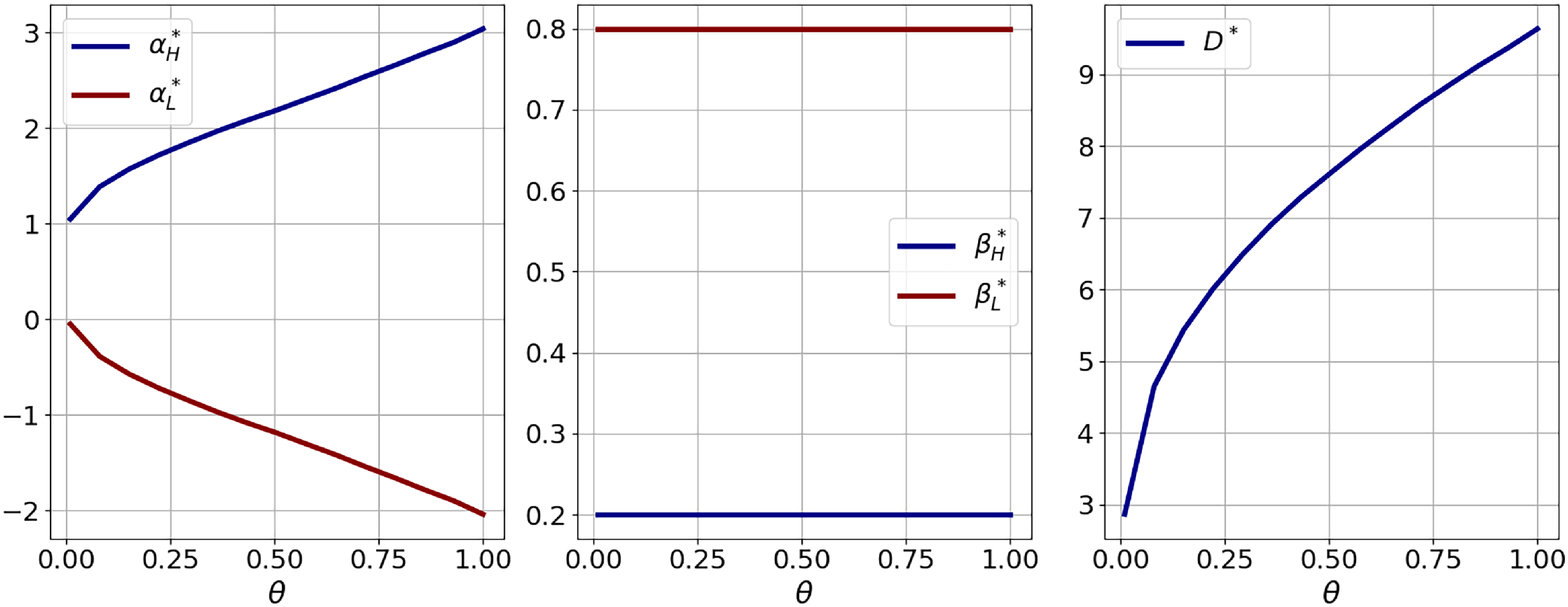
In the following, we further examine how the optimal parameters $(\alpha^*, \beta^*, D^*)$ vary with respect to the loading parameter $\theta$ under Scenario 1. First, Figure 4 presents the results without the IR constraint. We observe that $\alpha_H^*$ increases with the insurer’s loading factor $\theta$ . As expected, since $\alpha_H^*+\alpha_L^*=1$ , $\alpha_L^*$ follows the opposite trend. Additionally, we find that $\beta_H^*$ and $\beta_L^*$ remain independent of $\theta$ . This result is consistent with Equation (3.5) in Theorem 1, as the optimal $\beta^*$ depends solely on the values of $\gamma$ s. Moreover, $D^*$ increases with $\theta$ , indicating the pool’s greater willingness to share risk.

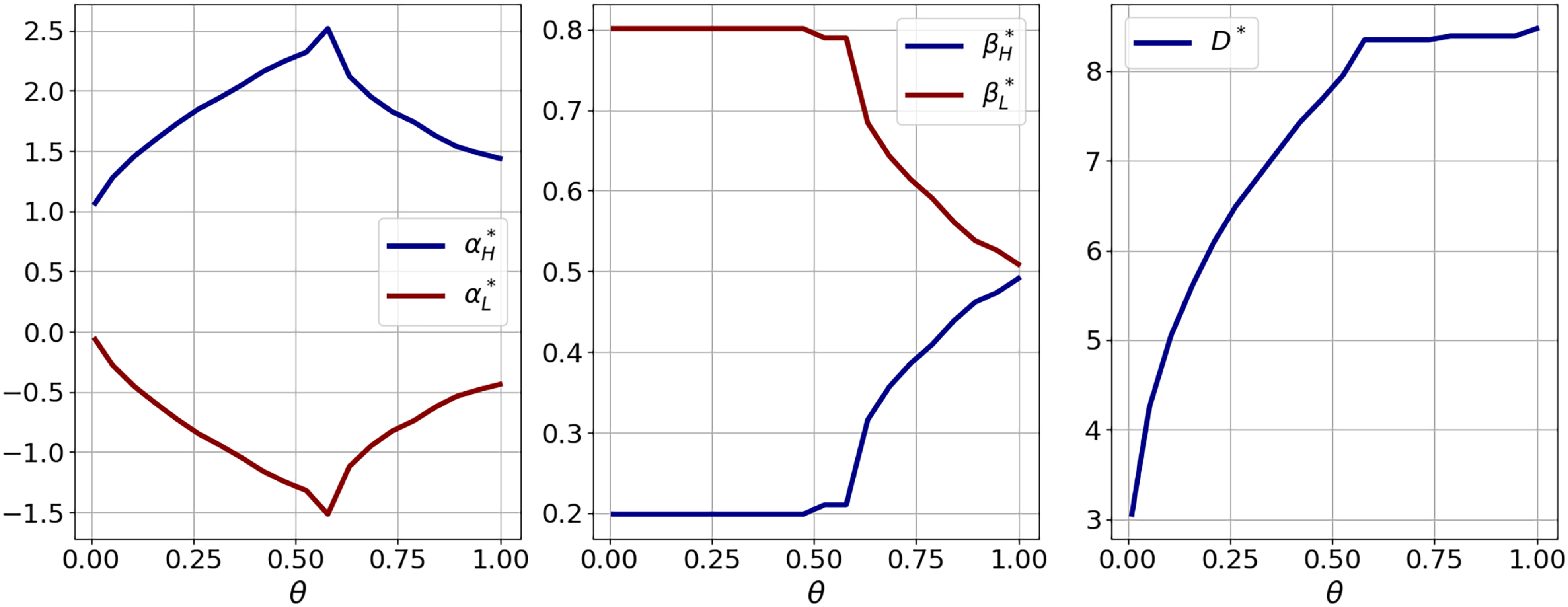
Second, Figure 5 presents the sensitivity analysis of the optimal contract parameters $(\alpha^*, \beta^*, D^*)$ under the IR constraint with respect to the loading parameter $\theta$ . The analysis reveals three distinct behavioral patterns. First, $\alpha_H^*$ exhibits a nonmonotonic relationship with $\theta$ , initially increasing before decreasing, while $\alpha_L^*$ follows the opposite trajectory, first decreasing then increasing; this phase transition occurs precisely when $\theta$ crosses the threshold at which the IR constraint becomes binding. Second, the $\beta^*$ parameters show threshold-dependent behavior: both $\beta_H^*$ and $\beta_L^*$ remain constant in the unconstrained regime but diverge significantly once the IR condition takes effect, with $\beta_H^*$ decreasing and $\beta_L^*$ increasing monotonically with $\theta$ . Finally, the optimal deductible $D^*$ increases monotonically with $\theta$ until the IR constraint becomes binding, after which it remains relatively stable. These results collectively demonstrate how the IR condition serves as a bifurcation point that fundamentally alters the sensitivity of optimal contract parameters to the loading factor.

Figure 5.

Sensitivity analysis of $\theta$ with IR condition.