In national-level studies of public social spending, many efforts have been made to explain why some countries consistently pursue more welfare-enhancing policies than others. From the perspective of institutional scholars, democratic institutions enable politicians to make credible policy commitments to the electorate through competitive elections, so citizens who prefer redistributive policies are able to influence policy decisions by electing their representatives, compared with non-democratic ones (Meltzer and Richard Reference Meltzer and Richard1981; Persson and Tabellini Reference Persson and Tabellini2000). The realization of redistributive policies in democracies, however, may only be observed in the long term (Huber et al. Reference Huber, Stephens, Mustillo and Pribble2008; Keefer and Vlaicu Reference Keefer and Khemani2008). This raises one empirical question: Does democracy matter for social welfare programs in the short term, in the long term, or both?
This article addresses this question by focusing on the estimation issues of dynamics of rarely changing variables such as political regimes in time-series cross-sectional (TSCS).Footnote 1 In the analysis of TSCS data or panel data, which have both intertemporal and cross-sectional variations, researchers are able to control for unobserved heterogeneity across units to eliminate omitted variable bias in estimation by including unit-specific effects.Footnote 2 However, it is problematic to estimate a panel model with a lagged dependent variable (LDV), time-invariant and/or rarely changing variables, and unit effects by two conventional approaches: fixed-effects (FE) models and random-effects (RE) models (Wooldridge Reference Wooldridge2002; Hsiao Reference Hsiao2003; Baltagi Reference Baltagi2005).
Building on the structure of simultaneous equation modeling and error-component formulations, a Bayesian simultaneous equation model (hereafter, BSEM) is developed here with hierarchical features that accommodate the correlation between the unit effects and explanatory variables, for which I focus on time-varying and rarely changing variables. Unlike conventional approaches, the BSEM provides additional information on the degree of the correlation. The complexity of this specification requires estimation with Markov chain Monte Carlo (MCMC) methods. A Bayesian approach offers flexibility for complex model specifications and resolves the inferential problems that arise in non-Bayesian multilevel models (MLMs) (Carlin and Louis Reference Carlin and Louis2000; Gill Reference Gill2008a).
To assess the performance of the BSEM presented in this article, I employ a Monte Carlo study, in which I compare the proposed model with alternative estimators in estimating the coefficients of correlated time-varying and rarely changing variables. The simulation results show that the proposed model not only performs as well as, or better than alternative estimators in terms of unbiasedness and efficiency, but also can estimate the correlation between covariates and the unit effects. The proposed model is applied to analyze the effects of political regimes on social spending in Latin America, where countries have different democratic experiences and different social welfare systems. This article finds evidence that democracy has a positive effect on social spending both in the short and long term.
This article has two primary contributions. First, methodologically, the proposed model in this article can deal with the problem of the correlation between the unit effects and covariates under the framework of multilevel modeling. Doing so, the proposed model is more efficient than the FE models and less biased than the RE models. Second, substantively, this article contributes to our understanding of the effects of political regimes on social spending in general. The evidence of positive democratic effects on social spending in Latin American countries support existing theories of comparative political economy that predict more redistributive policies in democracies.
The remainder of this article proceeds as follows. The A Model for Endogenous Rarely Changing Variables section discusses modeling dynamics of a endogenous, rarely changing variable, and a Bayesian approach to the model specification, followed by a Monte Carlo study in the Monte Carlo Simulations section. The Application: Social Spending in Latin America section presents the application of the proposed model to social security and welfare spending (SSW) in Latin America, and the Concluding Remarks section concludes.
A Model for Endogenous Rarely Changing Variables
Suppose that there exist TSCS data with a continuous outcome variable, y jt , and a rarely changing variable, w jt , for unit j=1, … , J measured at time t=1, … , T, which indicates a balanced TSCS data structure. A major advantage of TSCS data is that researchers are able to control for unobserved heterogeneity across units and/or through time to avoid omitted variable bias by including unit-specific and/or time-specific effects (Wooldridge Reference Wooldridge2002; Hsiao Reference Hsiao2003; Baltagi Reference Baltagi2005). For simplicity, I consider only unit heterogeneity in the model specification. Furthermore, to model dynamics, one standard approach is to include an LDV, y j(t−1), into the model. Thus, the model is specified as
 $$y_{{jt}} \,{\equals}\,\mu {\plus}\phi y_{{j(t{\minus}1)}} {\plus}\beta w_{{jt}} {\plus}\delta _{j} {\plus}{\varepsilon}_{{jt}} ,$$
where μ denotes the intercept, ϕ the autoregressive coefficient, β the coefficient parameter, δ
j
the unit-specific effects, and ε
jt
the error term. It is assumed that the error term is independently, identically distributed with mean 0 and finite variance
 $\sigma _{{\varepsilon}}^{2} $
.
When the inclusion of the LDV appropriately captures the dynamics of explanatory variables, autocorrelation can be eliminated (Beck and Katz Reference Beck and Katz1996, 2011; Keele and Kelly Reference Keele and Kelly2006). This works particularly well when covariates are rarely changing and their effects decay over time. To represent the decaying effects of covariates, it is assumed that the process {y jt } is stationary for individual units, i.e., formally, |ϕ|<1, which means that there is no unit roots. With the stationary assumption, the dynamic effects of a rarely changing variable on the outcome can be obtained by the dynamic multiplier, also referred to as the impulse response function in time-series analysis (see e.g., Hamilton Reference Hamilton1994; Enders Reference Enders2004).Footnote 3
When researchers are interested in the dynamics of slowly changing variables and specify a dynamic panel model, e.g., Equation 1, as my motivation stated in the first section, they face a quandary between FE and RE models. For those who prefer FE models, FE models not only provide inefficient estimates for rarely changing variables (Plümper and Troeger Reference Plümper and Troeger2007), but also give biased and inconsistent coefficient estimates for finite samples as the inclusion of the LDV violates the assumption of strict exogeneity of the regressors (Nickell Reference Nickell1981). For those who prefer RE models, which can be considered as a special case of MLMs, the consistency of parameter estimates of RE models depends not only on the assumption of the independence between the unit effects and covariates, but also on the initial conditions of the outcome variable (Anderson and Hsiao Reference Anderson and Hsiao1981; Anderson and Hsiao Reference Anderson and Hsiao1982; Hsiao Reference Hsiao2003).
It has been shown that the RE model for dynamic panel models is consistent, assuming that the initial values of outcomes (i.e., y j0) are treated as fixed constants (Anderson and Hsiao Reference Anderson and Hsiao1982; Sevestre and Trognon Reference Sevestre and Trognon1985). This property holds only if explanatory variables are not correlated with the unit effects or, at least, the correlation is explicitly modeled. A common approach to deal with the correlation between the unit effects and covariates is to include the within-group means of the covariates as group-level predictors suggested by Mundlak (Reference Mundlak1978). However, there is little discussion on finite sample properties of this approach for dynamic panel models in estimating correlated rarely changing variables although some literature implies that this approach works fine asymptotically (Anderson and Hsiao Reference Anderson and Hsiao1982; Hsiao Reference Hsiao2003).
Building on the structure of simultaneous equation models and error-component formulations, an RE-based model is proposed here to accommodate the dependence between the unit effects and rarely changing variables. This model not only explicitly deals with the problem of endogenous explanatory variables, but also maintains the advantages of multilevel modeling, e.g., the extension to models with random coefficients. For illustration, consider the model presented in Equation 1, which contains an LDV, a rarely changing variable, and the unit effects. The resulting analysis also holds for correlated time-varying variables and can be generalized to both static and dynamic panel models containing both exogenous and endogenous explanatory variables.
I start with the assumption that a rarely changing variable can be decomposed into three components: a mean effect, differences between units, and differences within units. Differences between units are effects specific to individual units, which do not vary over time, and differences within units are changes over time within a specific individual unit. Thus, the slowly changing variable can be expressed as
 $$w_{{jt}} \,{\equals}\,\zeta _{0} {\plus}\eta _{j} {\plus}\xi _{{jt}} ,$$
where ζ 0 denotes the mean effect, η j between differences, which can be treated as the “unit effects” for w jt , and ξ jt within differences.Footnote 4 Combining Equation 2 with Equation 1, we have a simultaneous equation model as follows:
 $$y_{{jt}} \,{\equals}\,\mu {\plus}\phi y_{{j(t{\minus}1)}} {\plus}\beta w_{{jt}} {\plus}\delta _{j} {\plus}{\varepsilon}_{{jt}} ,$$
 $$w_{{jt}} \,{\equals}\,\zeta _{0} {\plus}\eta _{j} {\plus}\xi _{{jt}} .$$
Equation 3 is an ordinary panel model for a continuous outcome variable and it is assumed that
 $${\varepsilon}_{{jt}} \mathop{\,\sim\,}\limits^{{{\rm iid}}} N(0,\sigma _{{\varepsilon}}^{2} ).$$
Note that ξ
jt
in Equation 4 denotes differences within units for a rarely changing variable. Although the distribution of ξ
jt
may be limited to certain values empirically, which depends on the operationalization of variables, ξ
jt
can be any positive or negative values theoretically. In other words, ξ
jt
ranges from negative infinity to positive infinity in general. Moreover, as the value of w
jt
rarely changes for a given unit j, ξ
jt
is highly likely to be 0. Based on these two general points, I assume that ξ
jt
follows a normal distribution with mean 0 and finite variance
 $\sigma _{\xi }^{2} $
, i.e.,
 $$\xi _{{jt}} \mathop{\,\sim\,}\limits^{{{\rm iid}}} N(0,\sigma _{\xi }^{2} ).$$
Next, to model the correlation across equations, i.e., the dependence between δ
j
and w
jt
, I assume that there exists a time-invariant, unobserved common factor related to some features of the individual units influencing both y
jt
and w
jt
through δ
j
and η
j
, respectively.Footnote
5
That is to say, the dependence between δ
j
and w
jt
results from the correlation between δ
j
and η
j
. Following the conventional approach in which the unit effects are assumed to be normally distributed with mean 0 and finite variance (Mundlak Reference Mundlak1978; Gelman and Hill Reference Gelman, Carlin, Stern and Rubin2007), it is assumed that the joint distribution for the vector
 $$\psi _{j} \,{\equals}\,{\rm }(\eta _{j} ,\delta _{j} )$$
is a bivariate normal distribution:
 $$(\eta _{j} ,\delta _{j} )\,\sim\,N_{2} ({\bf 0},{\bf \Omega }),\quad {\rm for}\quad j\,{\equals}\,1, \cdots ,J,$$
where the variance–covariance matrix is of the form
 $${\bf \Omega }\,{\equals}\,\left( {\matrix{ {\sigma _{\eta }^{2} } & {\sigma _{{\delta \eta }} } \cr {\sigma _{{\delta \eta }} } & {\sigma _{\delta }^{2} } \cr } } \right).$$
Consequently, the dependence between δ
j
and w
jt
is represented by the covariance σ
δη
. As our interest is the correlation between δ
j
and w
jt
, given Ω and
 $\sigma _{\xi }^{2} $
, we can simply derive this value by the definition of correlation given by
 $$\eqalignno{ {\rm corr}(\delta _{j} ,w_{{jt}} )\,{\equals}\, & {{{\rm Cov}(\delta _{j} ,w_{{jt}} )} \over {\sqrt {{\rm Var}(\delta _{j} ){\rm Var}(w_{{jt}} )} }}, \cr \,{\equals}\, & {{{\rm Cov}(\delta _{j} ,\eta _{j} )} \over {\sqrt {{\rm Var}(\delta _{j} ){\rm Var}(w_{{jt}} )} }}, \cr \,{\equals}\, & {{\sigma _{{\delta \eta }} } \over {\sqrt {\sigma _{\delta }^{2} (\sigma _{\xi }^{2} {\plus}\sigma _{\eta }^{2} )} }}. $$
The second line of Equation 9 is derived because the correlation between w jt and δ j in fact results from the correlation between η j and δ j .
The main distinction between Mundlak’s (Reference Mundlak1978) approach and the BSEM presented in this section is that the former provides no further information about the degree of the correlation between covariates and the unit effects while the latter does, given that both approaches explicitly model the correlation. The additional information gained from the BSEM over Mundlak’s approach is important for at least two reasons. First, the estimated correlation shows the extent of the dependence with regard to a particular covariate. With this information, we know which covariates suffer from the problem of endogeneity and how serious this problem is. Second, in practice, the information on the degree of the correlation shows us which variables are correlated to the features of the individual units that do not vary over time. When a covariate is highly correlated to the unit effects, it means that the differences in this covariate are mainly from the differences in the features of individual units. This information sometimes has theoretical meanings.
I estimate this model by a Bayesian approach, so I complete the model specification by defining the prior distribution. Let θ =( β , σ ε , ζ 0, σ ξ , Ω) denote the model parameters where β =(ϕ, μ, β)′. Following the conventional approach (Carlin and Louis Reference Carlin and Louis2000; Robert Reference Robert2001; Gelman et al. Reference Gelman and Hill2004), I use conjugate prior distributions for these parameters as follows:
 $$\sigma _{{\varepsilon}}^{2} \,\sim\,{\rm Inv}{\minus}{\rm Gamma}({{v_{0} } \mathord{\left/ {\vphantom {{v_{0} } 2}} \right. \kern-\nulldelimiterspace} 2},{{d_{0} } \mathord{\left/ {\vphantom {{d_{0} } 2}} \right. \kern-\nulldelimiterspace} 2}),$$
 $$\beta\! \mid\!\sigma _{{\varepsilon}}^{2} \,\sim\,N_{3} ({\mib{b}} _{0} ,\sigma _{{\varepsilon}}^{2} {\mib{B}} _{0} ),$$
 $$\sigma _{\xi }^{2} \,\sim\,{\rm Inv}{\minus}{\rm Gamma}(g_{0} \,/\,2,h_{0} \,/\,2),$$
 $$\zeta _{0} \!\mid\!\sigma _{\xi }^{2} \,\sim\,N(m_{0} ,\sigma _{\xi }^{2} \,/\,a_{0} ),$$
 $${\bf \bOmega }\,\sim\,{\rm Inv}{\minus}{\rm Wishart}(\nu _{0} ,{\bf \bLambda }_{0}^{{{\minus}1}} ),$$
where v
0, d
0,
b
0,
B
0, g
0, h
0, m
0, a
0, ν
0, and Λ
0 are hyperparameters, which can be assigned values to reflect prior information about the corresponding parameters or to give diffuse forms.Footnote
6
Furthermore, I assume priori independence of
 $({\bf \beta },\sigma _{{\varepsilon}}^{2} ),(\zeta _{0} ,\sigma _{\xi }^{2} )$
, and Ω and, therefore, our prior distribution of
θ
is given by
 $$\eqalignno{ \pi ({\bf \bitheta })\,{\equals}\,& IG\left( {\sigma _{{\varepsilon}}^{2} \mid {{v_{0} } \over 2},{{d_{0} } \over 2}} \right)N_{3} \left( {{\bf \beta } \mid \sigma _{{\varepsilon}}^{2} ,{\mib{b}}_{0} ,{\mib{B}}_{0} } \right) \cr & {\times}IG\left( {\sigma _{\xi }^{2} \mid {{g_{0} } \over 2},{{h_{0} } \over 2}} \right)N\left( {\zeta _{0} \mid \sigma _{\xi }^{2} ,m_{0} ,a_{0} } \right)IW\left( {{\bf \bOmega } \mid \nu _{0} ,{\bf \bLambda }_{0}^{{{\minus}1}} } \right). $$
Let
y
j
=(y
j1, y
j2, … , y
jT
)′,
y
j,−1=(y
j0, y
j1, … , y
j(T−1))′,
w
j
=(w
j1, w
j2,…,w
jT
)′,
 $${\mib \bixi } _{{\rm j}} {\rm \,{\equals}\,(}\xi _{j {\rm 1}} {\rm , }\xi _{j{\rm 2}} , \cdots ,\xi _{j\, t} {\rm )}'$$
, and
 $${\mib {\varepsilon}} _{j} \,{\equals}\,({\varepsilon}_{j 1} ,{\varepsilon}_{j 2} , \cdots ,{\varepsilon}_{j\,t} )'$$
be T×1 vectors of observations for unit j=1, 2, … , J. The simultaneous equation model has the form
 $$\left( {\matrix{ {{\bf w}_{j} } \cr {{\bf y}_{j} } \cr } } \right)\,{\equals}\,\left( {\matrix{ {\bf 0} & {\bf 0} \cr {\beta {\bf I}_{T} } & {\bf 0} \cr } } \right)\left( {\matrix{ {{\bf w}_{j} } \cr {{\bf y}_{j} } \cr } } \right){\plus}\left( {\matrix{ {\zeta _{0} {\bf I}_{T} } & {\bf 0} \cr {\mu {\bf I}_{T} } & {\phi {\rm I}_{T} } \cr } } \right)\left( {\matrix{ {\mib{e}} \cr {{\mib{y}} _{{j,{\minus}1}} } \cr } } \right){\plus}\left( {\matrix{ {\mib{e}} & {\tilde{0}} \cr {\tilde{0}} & {\mib{e}} \cr } } \right)\left( {\matrix{ {\eta _{j} } \cr {\delta _{j} } \cr } } \right){\plus}\left( {\matrix{ {{\mib{\bixi }} _{j} } \cr {{\mib{{\bivarepsilon}}} _{j} } \cr } } \right),$$
where 0 is a T×T matrix, e=(1, … , 1)′ is a T×1 vector,
 $\tilde{0}\,{\equals}\,(0,\: \cdots \:,0)'$
is a T×1 vector. The multivariate regression representation of the structural form is given by
 $${\mib{Y}} _{j} \,{\equals}\,{\mib{BY}} _{j} {\plus}{\bf \Gamma }{\mib{X}} _{j} {\plus}{\mib{Z}} \bipsi _{j} {\plus}{\mib{U}} _{j} ,$$
where
 $$\bipsi _{j} \,{\equals}\,{\rm }(\eta _{j} ,\delta _{j} )',$$
U
j
~N(0, Σ), and
 $${\bf \Sigma }\,{\equals}\,\left( {\matrix{ {\sigma _{\xi }^{2} {\bf I}_{T} } & {\rm 0} \cr {\rm 0} & {\sigma _{{\epsilon}}^{2} {\bf I}_{T} } \cr } } \right).$$
Also, let
y
=(
y
1, … ,
y
J
),
w
=(
w
1, … ,
w
J
), and
 $${\mib \bipsi } \,{\equals}\,({\mib \bipsi } _{1} , \cdots ,{\mib \bipsi } _{J} )$$
. The likelihood function for the simultaneous equation model denoted by
 $$p({\mib{w},\,\mib{y}}\,\mid\,\bipsi ,\,\bitheta )$$
has the form
 $$p({\mib{w}} ,{\mib{y}} \mid \bipsi ,{\mib{\bitheta }} )\,{\equals}\,\prod\limits_{j\,{\equals}\,1}^J p({\mib{w}} _{j} ,{\mib{y}} _{j} \mid \bipsi ,{\mib{\bitheta }} ),$$
where
 $$p({\mib{w}} _{j} ,{\mib{y}} _{j} \mid {\mib \bipsi } ,{\mib \bitheta } ){\rm }\,{\equals}\,N_{{2T}} ({\mib{BY}} _{j} {\plus}{\bf \Gamma } {\mib{X}} _{j} {\plus}{\mib{Z}} \bipsi _{j} ,{\bf \sum} )N_{2} (\bipsi _{j} \mid{\bf 0},\Omega ).$$
From the Bayes theorem, the joint posterior distribution of interest,
 $$\pi ({\mib \theta } \,\mid\,{\mib{y}} ,{\mib{w}} ,{\mib \bipsi } )$$
, is as follows:
 $$\pi ({\mib \bitheta } \mid {\mib{y}} ,{\mib{w}} ,{\mib \bipsi } ) \propto p ({\mib{y}} ,{\mib{w}} \,\mid\,{\mib \bipsi } ,{\mib{\bitheta }} )p({\mib \bipsi } \mid {\mib{\bitheta }} )\pi ({\mib{\bitheta }} ).$$
This joint distribution is of a type that can be efficiently processed by MCMC methods (see Gelfand and Smith Reference Gelfand and Smith1990; Casella and George Reference Casella and George1992; Chib and Greenberg Reference Chib and Greenberg1995), which can be implemented in computer programs such as WinBUGS (Lunn et al. Reference Lunn, Thomas, Best and Spiegelhalter2000) and JAGS (Plummer Reference Plummer2003).
Monte Carlo Simulations
In this section, I employ Monte Carlo simulations to assess the finite sample properties of the BSEM, compared with alternative estimators that have been proposed or suggested to estimate correlated explanatory variables.
Simulation Design
The data generation process (DGP) for the simulations is as follows:
 $$y_{{jt}} \,{\equals}\,\mu {\plus}\phi y_{{j(t{\minus}1)}} {\plus}\alpha _{1} x_{{1jt}} {\plus}\alpha _{2} x_{{2jt}} {\plus}\alpha _{3} x_{{3jt}} {\plus}\beta _{1} w_{{1jt}} {\plus}\beta _{2} w_{{2jt}} {\plus}\beta _{3} w_{{3jt}} {\plus}\delta _{j} {\plus}{\varepsilon}_{{jt}} ,$$
where x 1, x 2, and x 3 are time-varying variables and w 1, w 2, and w 3 are rarely changing variables, δ j denotes the unit effects, and ε jt the error term. The two groups of variables except w 3 are drawn from a normal distribution with different means and variances; δ j is normally distributed with mean 0 and variance 1; the error term ε jt is assumed to be white noise and drawn from a standard normal distribution. Among the covariates, x 3 and w 3 are correlated with the unit effects δ j and, thus, x 3, w 3, δ, and ε vary for each replication while x 1, x 2, w 1, and w 2 are fixed across all experiments. In the experiments, the correlation between x 3 and the unit effects, corr(x 3, δ j ), and the correlation between w 3 and the unit effects, corr(w 3, δ j ), are varied. In specific, corr(x 3, δ j )={0, 0.1, 0.2, … , 0.9} and corr(x 3, δ j )={0, 0.1, 0.2, … , 0.9}.Footnote 7
The true values of the coefficients are held constant throughout all experiments as follows:
 $$\mu \,{\equals}\,1,\,\phi \,{\equals}\,0.8,\,\alpha _{1} \,{\equals}\,0.5,\,\alpha _{2} \,{\equals}\,2,\,\alpha _{3} \,{\equals}\,{\minus}1.5,\,\beta _{1} \,{\equals}\,{\minus}2.5,\,\beta _{2} \,{\equals}\,1.8,\,\beta _{3} \,{\equals}\,3.$$
I simulate the data with different numbers of time periods T={15, 30, 60} and fixed number of units J=20. The number of replications is 500 for each experiment. Moreover, another experimental design is conducted in which the data are simulated with different numbers of units J={40, 60} and fixed number of time periods T=30. For this design, the number of replications is 100.
The DGP presented in Equation 21 follows the simulation design in Plümper and Troeger (Reference Plümper and Troeger2007) but differs in three fundamental respects. First, the unit effects vary across replications for each experiment, which account for random variation in the unit effects (Breusch et al. Reference Breusch, Ward, Nguyen and Kompas2011). Second, the rarely changing variables I consider are persistent for the rest of periods under analysis once they change at a certain (randomly assigned) time point. Finally, the dynamics of explanatory variables are taken into account by the inclusion of the LDV in the DGP.
The BSEM employed here contains two endogenous covariates, x 3 and w 3, which is an extension of the one discussed in the A Model for Endogenous Rarely Changing Variables section. This Bayesian model with vague priors is estimated with MCMC techniques and is implemented in JAGS 3.1.0 called from R version 3.1.0 (Su and Yajima Reference Su and Yajima2012).Footnote 8 The estimation was performed with three parallel chains of 10,000 iterations each. The first half of the iterations were discarded as a burn-in and five as thinning, and thus 3000 samples in total were generated. The convergence of Markov chains was tested by standard diagnostic tools such as Geweke, Gelman-Rubin, Raftery-Louis, and Heidelberger-Welch (Gill Reference Gill2008b) and was conducted by an easy to use R function superdiag that integrates all of the standard empirical diagnostics (Tsai and Gill Reference Tsai and Gill2012). The results show no evidence of non-convergence.
The alternative estimators considered include the pooled ordinary least squares (OLS) estimator, the FE estimator, the fixed-effects vector decomposition (FEVD) estimator (Plümper and Troeger Reference Plümper and Troeger2007), the RE model, and a MLM with the within-group means of the correlated variables (Mundlak Reference Mundlak1978; Gelman Reference Gelman2006). This procedure is implemented in R: the FE and RE models are estimated through the plm package (Croissant and Millo Reference Croissant and Millo2008); the MLM is estimated by the restricted maximum likelihood estimation through the lme4 package (Bates, Maechler and Ben Reference Bates, Maechler, Bolker and Walker2015).Footnote 9
To compare competing estimators, I follow the literature in reporting the average bias and the root mean squared error (RMSE) of estimates. To avoid the bias to be canceled out, I calculate the absolute value of bias (hereafter, AVB). The RMSE captures both the bias and efficiency of the estimators calculated based on the formula
 $\scale 85%\sqrt {{{\mathop{\sum}\nolimits_{s\,{\equals}\,1}^R \left( {\hat{\beta }^{{(s)}} {\minus}\beta _{{{\rm true}}} } \right)^{2} } \over R}} $
, where
 $\hat{\beta }^{{(s)}} $
denotes the estimate, s in the superscript denotes the sth replicate within R replications, and β
true is the true value.
Moreover, the uncertainty associated with simulation results is reported along with the estimates of AVB and RMSE (Koehler, Brown and Haneuse Reference Koehler, Brown and Haneuse2009). Let θ denote some target quantities of interest, i.e., AVB and RMSE, and
 $\hat{\theta }_{R} $
the estimate of θ from a Monte Carlo simulation with R replications. The variability between simulations, also called the Monte Carlo error (MCE), is defined as the standard deviation of the Monte Carlo estimator:
 $${\rm MCE}(\hat{\theta }_{R} )\,{\equals}\,\sqrt {{\rm Var}(\hat{\theta }_{R} )} .$$
That is to say, MCE(AVB R ) and MCE(RMSE R ) of a number of coefficient parameters are presented in the simulation results to show the variation of the Monte Carlo sampling distribution.
Results of Simulation
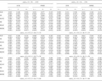
In Table 1, I report the AVB and RMSE over ten experiments for three different designs: T={15, 30, 60} with J=20. The results of experiments in which the correlation between the time-varying variable x 3 and the unit effects δ is varied are displayed from the second to the seventh columns; those in which the correlation between the rarely changing variable w 3 and the unit effects δ is varied are displayed in the eighth to the 13th columns. Notice that in the former corr(w 3, δ j ) is fixed at the value of 0.3 while in the latter corr(x 3, δ j ) is fixed at the value of 0.3.
Absolute Value of Bias (AVB) and Root Mean Squared Error (RMSE) over 500 Replications Times Ten Experiments with T Varied

Note: Monte Carlo errors are presented in parentheses.
OLS=ordinary least squares; FE=fixed effects; FEVD=fixed-effects vector decomposition; RE=random effects; MLM=multilevel models; BSEM=Bayesian simultaneous equation model.
The results in Table 1 are summarized as follows. First, on average, the pooled OLS produces the poorest estimates in terms of AVB and RMSE. As we know and the results confirm, the correlation between the LDV and the unit effects would seriously bias the pooled OLS estimator. Furthermore, the correlation between covariates and the unit effects exacerbates the problem. The magnitude of AVB and RMSE does not decrease as T increases.
Second, among these six estimators, the FEVD estimator produces estimates with the largest AVB and RMSE for the rarely changing variable in all cases while its estimates for the LDV and the time-varying variable are exactly the same with those under the FE model. The results indicate that the FEVD does not perform well for estimating rarely changing variables in dynamic panel data models.
Third, the RE is more biased than the FE in estimating correlated covariates x 3 and w 3 while the RE is more efficient than the FE in estimating slightly correlated covariates, i.e., corr(x 3, δ j )=0.3 or corr(w 3, δ j )=0.3. As the correlation is modeled under the MLM, the MLM and the FE perform equally well in estimating coefficients for the LDV and correlated covariates in terms of AVB and RMSE. In other words, when the correlation between the unit effects and covariates is modeled by Mundlak’s (Reference Mundlak1978) approach, the MLM is less biased at the expense of efficiency.
Last but not least, the BSEM performs as well as, or better than the FE, RE, and MLM in terms of AVB and RMSE. We can see that, in almost all of the cases, the BSEM is the least biased and the most efficient estimator. These properties can be more clearly observed when T is small.
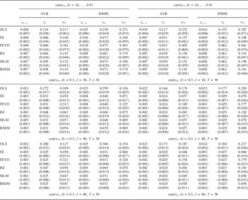
In Table 2, I report the AVB and RMSE over ten experiments for three different designs: J={10, 40, 60} with T=30. Combining the results in Table 2 and the results in the middle block of Table 1 in which J=20 and T=30, we can see how the performances of these estimators change as the number of units increases. We find that the results are similar to those summarized above: the pooled OLS produces the poorest estimates and does not perform better as J increases; the FEVD does not perform well for estimating rarely changing variables in dynamic panel data models; the RE is more biased than the FE, MLM, and BSEM; the MLM and BSEM performs equally well with the FE in terms of AVB but are more efficient than the FE; the BSEM performs better than the MLM especially when J is small, e.g., J=10.
An Absolute Value of Bias (AVB) and Root Mean Squared Error (RMSE) over 100 Replications Times Ten Experiments with J Varied

Note: Monte Carlo errors are presented in parentheses.
OLS=ordinary least squares; FE=fixed effects; FEVD=fixed-effects vector decomposition; RE=random effects; MLM=multilevel models; BSEM=Bayesian simultaneous equation model.
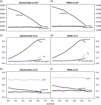
I then show the effects of the correlation on the AVB and RMSE of the estimates for the LDV, time-varying variable x 3, and rarely changing variable w 3. To save space, I only present the results from the design where J=20 and T=30, but the results remain the same for T={15, 60} with J fixed and J={40, 60} with T fixed. Figure 1 presents the AVB and RMSE of the six estimators for the LDV, x 3, and w 3 when corr(x 3, δ j ) is varied and corr(w 3, δ j ) is fixed at the value of 0.3. The three panels on the left-hand side [(a), (c), and (e)] show the comparison in terms of AVB and, as can be seen, the pooled OLS produces estimates of the LDV and x 3 with the largest AVB. The RE performs worse for strongly correlated covariate x 3. The FEVD estimator has the poorest estimates of rarely changing variables and the FE, MLM, and BSEM perform more or less equally well in estimating all of these three variables no matter what the size of the correlation is.
Change in the absolute value of bias and root mean squared error (RMSE) over variations in the correlation between the unit effects and the time-varying variable x 3; corr(w 3, δ j )=0.3, J=20, and T=30 Note: LDV=lagged dependent variable; OLS=ordinary least squares; FE=fixed effects; FEVD=fixed-effects vector decomposition; RE=random effects; MLM=multilevel models; BSEM=Bayesian simultaneous equation model.

Furthermore, the same pattern appears in the RMSE of these estimators represented in the three panels on the right-hand side of Figures 1(b), 1(d), and 1(f). Simply put, the pooled OLS has the largest RMSE for the LDV and time-varying variable x 3 while the FEVD estimator performs poorly for the estimate of rarely changing variable w 3. The RE has poor performance in RMSE for the covariate strongly correlated to the unit effects. The BSEM performs equally well with the FE and MLM.
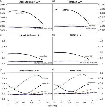
Figure 2 presents the AVB and RMSE of the six estimators for the LDV, time-varying variable x 3, and rarely changing variable w 3 when corr(x 3, δ j ) is fixed at the value of 0.3 and corr(w 3, δ j ) is varied. It shows that, in general, the pooled OLS has the largest AVB and inefficient estimates of the LDV and x 3; the RE has biased and inefficient estimates for the LDV and w 3; the FEVD performs poorly in terms of the AVB and RMSE in estimating the coefficient of w 3. The FE, MLM, and BSEM perform equally well in estimating the LDV, x 3, and w 3.
Change in the absolute value of bias and root mean squared error (RMSE) over variations in the correlation between the unit effects and the rarely changing variable w 3; corr(x 3, δ j )=0.3, J=20, and T=30 Note: LDV=lagged dependent variable; OLS=ordinary least squares; FE=fixed effects; FEVD=fixed-effects vector decomposition; RE=random effects; MLM=multilevel models; BSEM=Bayesian simultaneous equation model.

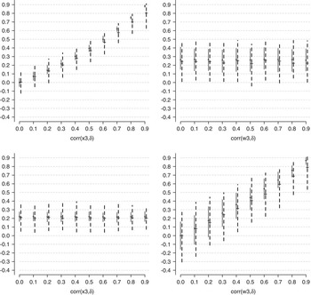
Finally, I present the estimates of the correlation between the unit effects and the time-varying variable and rarely changing variable from the proposed model. To save space, I only show the results from the design where T=30 and J=20. In Figure 3, the two panels on the top are from the design where corr(x 3, δ j ) is varied while corr(w 3, δ j ) is fixed at the value of 0.3; the two panels at the bottom are from the design where corr(x 3, δ j ) is fixed at the value of 0.3 while corr(w 3, δ j ) is varied. Moreover, the solid lines represent the 90 percent highest posterior density (HPD) intervals of the correlation between the unit effects and covariates from generated data while the dotted lines represent the 90 percent HPD intervals of the estimated correlation parameters. As can be seen in Figure 3, the estimates of correlation between the unit effects and the time-varying variable x 3 and those between the unit effects and rarely changing variable w 3 are approximately close to those in the generated data.Footnote 10 As the dotted lines represent the estimates, they have larger uncertainty than the simulated correlation coefficients. But the wide range of uncertainty decreases as J or T increases, which is not shown here to save space.
The 90 percent highest posterior density intervals of the simulated and estimated correlations between the unit effects and the covariates x 3 and w 3 for T=30 and J=20 Note: The plus signs denote the median. The solid lines present the correlation from the simulated data while the dotted lines present the estimates of correlation.

In short, the proposed model not only performs as well as, or better than classical estimators in estimating coefficients for correlated covariates in terms of bias and efficiency especially when J or T is small, but also provides estimates for the correlation between the unit effects and covariates. Therefore, when the sample size is small or the degree of the correlation between the unit effects and covariates is of interest, the proposed model is preferred to the conventional estimators such as the FE models which eliminate the unit effects, and the RE models which assume no correlation.
Robustness Check for Distributional Assumptions
One concern about the simulation results is that the setup of a bivariate normal distribution for δ j and x 3j matches the model assumption. In this subsection, I conduct a robustness analysis to check whether the data are simulated in favor of the proposed model and against the alternative estimators. Instead of drawing samples from a standard normal distribution, I draw the samples of δ j from a uniform distribution in the interval between −2 and 2. Then, the unit-level covariates x 3j and w 3j are generated based on the assigned values of correlation and the individual-level samples x 3jt and w 3jt are generated in turn, which is the same procedure as that is stated in the Simulation Design section (and in footnote 7 for details). By drawing samples of δ j from a uniform distribution, the joint distribution of δ j and x 3jt is a bimodal distribution rather than a bivariate normal distribution. The comparison between alternative estimators is conducted under the setting that J=20, T=15, and R=100.
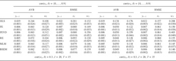
The results are shown in Table 3, which indicate that the performances of these estimators are consistent to what we find in the experiment with J=20 and T=15 presented in the top block of Table 1. The results remain the same when J or T is changed. Simply put, the results in Table 3 suggest that the changes in the distributional setup for the joint distribution of (δ j , x 3jt ) and that of (δ j , w 3jt ) do not influence the estimates. These results indicate that the BSEM still performs well even if the distributional assumptions of the BSEM are not matched by the simulation design, which implies that the simulation results are quite robust.
Absolute Value of Bias (AVB) and Root Mean Squared Error (RMSE) over 100 Replications Times Ten Experiments with Joint Distributions Changed

Note: Monte Carlo errors are presented in parentheses.
OLS=ordinary least squares; FE=fixed effects; FEVD=fixed-effects vector decomposition; RE=random effects; MLM=multilevel models; BSEM=Bayesian simultaneous equation model.
Sensitivity Analysis for the Choice of Priors
As discussed in the A Model for Endogenous Rarely Changing Variables section, one of the advantages of the proposed model against alternative estimators is that the BSEM can estimate the correlation between covariates and the unit effects. The major component for the estimation of correlation lies in the variance–covariance matrix Ω, which is assumed to be an inverse Wishart distribution with the degrees of freedom ν 0 and the scale matrix Λ 0. In both the simulation and the application, these hyperparameters of the inverse Wishart distribution are assigned values to be an uninformative prior for the correlation. In specific, suppose that Ω is a p×p matrix. The degree of freedom ν 0 is set to be p+1 and the scale matrix Λ 0 is an identity matrix I p , which implies a uniform distribution for the correlation.
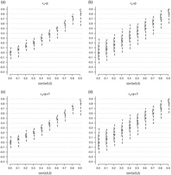
To check the sensitivity to the choice of this parameterization, I use three different parameterizations for the degrees of freedom while the scale matrix is fixed to an identity matrix I p : ν 0={p, p+3, p+7}, where p=3 in the simulation. The sensitivity analysis is conducted under the setting that J=20, T=15, and R=100. To save space, I only present the 90 percent HPD intervals of varied correlations for the designs where ν 0=p and p+7 displayed in Figure 4.Footnote 11 As can be seen, panels (a) and (c) in Figure 4 show the same pattern as the upper-left panel in Figure 3, which suggests that the estimated correlations are close to the simulated ones although the BSEM underestimates the correlation when the correlation is high. By the same token, panels (b) and (d) in Figure 4 show the same pattern as the bottom-right panel in Figure 3. In sum, these results show that the posterior distribution of correlation parameters from the BSEM is not affected by the choice of prior values.
The 90 percent highest posterior density intervals of the simulated and estimated correlation coefficients between the unit effects and the covariates for T=30 and J=20 Note: The plus signs denote the median. The solid lines present the correlation from the simulated data while the dotted lines present the estimates of correlation.

Application: Social Spending in Latin America
Previous studies on democracy and social welfare policy focus on Latin American countries because, first, there is great variation in social welfare systems among Latin American countries and, second, most Latin American countries experienced regime change between democracy and authoritarianism. However, the empirical results are not consistent. For example, while some studies show that democratic regimes tend to spend more on overall social programs than authoritarian regimes (Brown and Hunter Reference Brown and Hunter1999; Avelino, Brown and Hunter Reference Avelino, Brown and Hunter2005), others find no robust evidence that democracy has an impact on aggregate social expenditures (Kaufman and Segura-Ubiergo Reference Kaufman and Segura-Ubiergo2001). Moreover, for disaggregate spending, some find that democracy has a positive effect on social security spending in the long term (Huber et al. Reference Huber, Stephens, Mustillo and Pribble2008), while others do not find strong evidence in either the short term or the long term (Kaufman and Segura-Ubiergo Reference Kaufman and Segura-Ubiergo2001; Avelino, Brown and Hunter Reference Avelino, Brown and Hunter2005).
The inconsistent results in previous studies may result from at least two methodological issues. First, the slowly changing property of political regimes are not explicitly illustrated and different model strategies are used. Some of these studies include an LDV to correct for serial correlation (Kaufman and Segura-Ubiergo Reference Kaufman and Segura-Ubiergo2001; Avelino, Brown and Hunter Reference Avelino, Brown and Hunter2005). Some other studies consider the long-term properties of political regimes, but inappropriately model the long-term effects of democracy by cumulating yearly values of democracy variable (Huber et al. Reference Huber, Stephens, Mustillo and Pribble2008).
Second, the absence of country-specific effects in statistical models is one of the problems in past empirical research (Ross Reference Ross2006). One of the reasons to exclude unit effects is that these unit effects influence the coefficients of factors that vary mainly between countries (Plümper, Troeger and Manow Reference Plümper, Troeger and Manow2005). As discussed before, excluding the unit effects may be at the risk of having omitted variable bias, which leads to invalid inferences. Furthermore, as discussed in the A Model for Endogenous Rarely Changing Variables section, it is better to include an LDV and unit effects into model specifications to evaluate the effects of democracy on social welfare spending because it is believed that the effects of democracy is distributed across several extended time periods.
Data and Measurements
I apply the BSEM presented in the A Model for Endogenous Rarely Changing Variables section to analyze social spending in Latin America, which handles the above issues. The data set I use was collected by Huber et al. (Reference Huber, Stephens, Mustillo and Pribble2008).Footnote 12 This data set covers a number of political and economic variables in 18 Latin American countries from 1970 to 2000. In this application, the outcome variable is SSW, and the main explanatory variable is the level of democracy.
Before discussing the results of analysis, two important points need to be observed. First, SSW is measured as a percentage of gross domestic product (GDP). As it is bounded between 0 and 100 percent, we can argue that the proportion of GDP spent on social security is stationary (Beck and Katz Reference Beck and Katz2011). Second, the distribution of social security spending is right-skewed, so I use the logarithm transformation, which is better described by a normal distribution.Footnote 13
The level of democracy (DEM), which is rarely changing, is measured by the Polity index ranging from −10 to 10 with 10 as the highest degree of democracy (Marshall, Jaggers and Gurr Reference Marshall, Jaggers and Gurr2010). I also include several control variables that may influence social spending discussed in the literature. These control variables are gross domestic production per capita (GDPPC) (million US dollars) adjusted for purchasing power parities, the percentage of population that lives in the urban area (UBNPOP), the percentage of aged population (POP65), export and import as a percentage of GDP as a measurement of trade openness (TRADE), and foreign direct investment (FDI) as a percentage of GDP.Footnote 14
As I am not sure which covariate is correlated with the unit effects, I model all of them. Therefore, the simultaneous equation model is given by Equation 23:
 $$\eqalignno{ {\rm ln}({\rm SSW}_{{jt}} )\,{\equals}\, & \beta _{0} {\plus}\phi {\rm ln}({\rm SSW}_{{j(t{\minus}1)}} ){\plus}\beta _{1} {\rm DEM}_{{jt}} {\plus}\beta _{2} {\rm GDPPC}_{{jt}} {\plus}\beta _{3} {\rm UBNPOP}_{{jt}} \cr & {\plus}\beta _{4} {\rm POP}65_{{jt}} {\plus}\beta _{5} {\rm TRADE}_{{jt}} {\plus}\beta _{6} {\rm FDI}_{{jt}} {\plus}\delta _{j} {\plus}{\varepsilon}_{{jt}} , \cr {\rm DEM}_{{jt}} \,{\equals}\, & {\rm \zeta }_{1} {\plus}\eta _{{1j}} {\plus}{\rm \xi }_{{1jt}} , \cr {\rm GDPPC}_{{jt}} \,{\equals}\, & {\rm \zeta }_{2} {\plus}\eta _{{2j}} {\plus}{\rm \xi }_{{2jt}} , \cr {\rm UBNPOP}_{{jt}} \,{\equals}\, & {\rm \zeta }_{3} {\plus}\eta _{{3j}} {\plus}{\rm \xi }_{{3jt}} , \cr {\rm POP}65_{{jt}} \,{\equals}\, & {\rm \zeta }_{4} {\plus}\eta _{{4j}} {\plus}{\rm \xi }_{{4jt}} , \cr {\rm TRADE}_{{jt}} \,{\equals}\, & {\rm \zeta }_{5} {\plus}\eta _{{5j}} {\plus}{\rm \xi }_{{5jt}} , \cr {\rm FDI}_{{jt}} \,{\equals}\, & {\rm \zeta }_{6} {\plus}\eta _{{6j}} {\plus}{\rm \xi }_{{6jt}} . $$
This model is estimated with MCMC techniques and implemented in JAGS 3.1.0 called from R (R2jags).Footnote 15
Results of Analysis
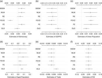
The results of the analysis of social spending are displayed in Figures 5–7. Figure 5 presents the intervals of 90 percent level for explanatory variables from the six estimators discussed in the Monte Carlo Simulations section. We can see that, first, in general the BSEM, FE, and MLM provide very similar results for the estimates for these covariates,Footnote 16 which suggest that democracy, GDP per capita, and the urban population matter for the outcome variable. In specific, democracy and the urban population have a positive effect while GDP per capita has a negative effect on social spending.
Determinants of social security spending, 1971–2000 Note: BSEM=Bayesian simultaneous equation model; MLM=multilevel models; RE=random effects; FEVD=fixed-effects vector decomposition; FE=fixed effects; OLS=ordinary least squares; GDPPC=gross domestic production per capita; FDI=foreign direct investment.

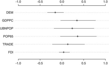
The 90 percent highest posterior density of estimated correlation between unit effects and covariates Note: DEM=democracy; GDPPC=gross domestic production per capita; UBNPOP=percentage of population that lives in the urban area; POP65=percentage of aged population; TRADE=measurement of trade openness; FDI=foreign direct investment.

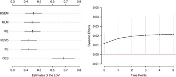
Estimates of the autoregressive coefficient and dynamic effects of political regimes on social spending. The solid lines represent 90 percent credible intervals Note: BSEM=Bayesian simultaneous equation model; MLM=multilevel models; RE=random effects; FEVD=fixed-effects vector decomposition; FE=fixed effects; OLS=ordinary least squares; LDV=lagged dependent variable.

Second, the estimate for democracy under the FEVD is negative, which is extremely different from the results in alternative estimators. The findings in the simulations tell us that this may be misleading as the FEVD is biased for rarely changing variable. Moreover, we also observe that the FEVD provides smaller uncertainty of estimates than the FE (Breusch et al. Reference Breusch, Ward, Nguyen and Kompas2011), which leads to incorrect inferences, e.g., a negative effect of democracy and a positive effect of the aged population and trade.
Finally, the estimates for democracy under the pooled OLS and RE are somewhat different from those under the BSEM, FE, and MLM. As the simulation results suggest, it is possible that the level of democracy is correlated to the unit effects based on the findings in the simulations. This situation also occurs for GDP per capita and the aged population.
To check the possibility of correlation between these variables and the unit effects, I rely on the 90 percent credible intervals of the estimated correlations provided by the BSEM presented in Figure 6. As can be seen, the posterior distribution of the estimated correlation between the unit effect and the level of democracy mainly lies in the negative region, which implies a negative correlation. In contrast, Figure 6 shows that the other five variables are positively correlated with the unit effects, among which the 90 percent credible intervals of correlation for GDPPC and POP65 mainly lie in the positive region although the intervals are wide. In short, the results suggest that the level of democracy, GDP per capita, and the aged population are slightly or moderately correlated to the unit effects. In other words, the results imply that the unobserved, time-invariant features of individual countries simultaneously influence social spending, political development, economic development, and the aged population.
Figure 5 shows that democracy matters for social spending. In a dynamic model, it basically means that democracy has an immediate effect on social provision policy. To see dynamic effects, one should consider the dynamic multiplier, which involves the coefficient of the LDV, ϕ (Keele and Kelly Reference Keele and Kelly2006). The left panel in Figure 7 shows the 90 percent intervals of the LDV from the six estimators. As can be seen, the estimates of the LDV from five estimators are almost equivalent except for that from the pooled OLS. It is well known that the estimate of the LDV is biased upward under the pooled OLS, which is observed in Figure 7. Taking the estimates from the BSEM, the right panel in Figure 7 presents the dynamic effects of democracy over six time periods when the Polity scores increase 1 unit. As can be seen, the posterior probability of the effect of democracy on social spending is over 90 percent. This implies that, for a given country, when the level of democracy increases, social spending increases as well. Overall, the evidence shows that democratic regimes have a positive effect on social spending in either the short term or the long term.
Concluding Remarks
Existing literature argues that democracies pursue more welfare-enhancing policies than non-democracies. Recently, some studies argue that the realization of redistributive policies in democracies may be observed in the long term (Keefer and Khemani Reference Keefer and Vlaicu2005; Keefer and Vlaicu Reference Keefer and Khemani2008). The empirical evidence of how political regimes affect redistributive policies, however, is inconsistent. Following studies of political regimes and redistributive policies in Latin America, this article examines the dynamic effects of political regimes on social programs by focusing on estimating the effects of rarely changing variables within a Bayesian framework.
The dynamic effects of rarely changing variables such as the level of democracy are often of great interest in the study of political economy. Nevertheless, the classical estimators are problematic when estimating the effects of time-invariant and rarely changing variables along with unit effects, the control of which is important in the analysis of welfare states (Kaufman and Segura-Ubiergo Reference Kaufman and Segura-Ubiergo2001; Ross Reference Ross2006). This article shows the flexibility and advantages of the Bayesian approach to estimating the coefficients of endogenous explanatory variables along with the parameters of the correlation between the unit effects and covariates. The finite sample properties of the proposed model and alternative estimators that are widely applied to panel data analyses are explored in Monte Carlo simulations. The results show that the proposed model not only performs as well as, or better than alternative estimators in terms of bias and efficiency, but also provides additional information on the degree of the correlation between the unit effects and covariates, which will not be discovered without the proposed model. Applying the BSEM to the study on social spending in Latin America, this article finds evidence that political regimes affect social welfare spending both in the short and long terms.
For future research, first, the proposed model can be applied to studies in which researchers are interested in the long-term effects of political institutions such as the effect of centralized wage bargaining on income inequality (Scheve and Stasavage Reference Scheve and Stasavage2009). Second, it would be useful to model heterogeneous coefficients and account for the correlated predictors at the group level as we have substantive (Western Reference Western1998; Beck and Katz Reference Beck and Katz2007) and methodological (Nerlove Reference Nerlove1971; Pesaran and Smith Reference Pesaran and Smith1995; Hsiao Pesaran and Tahmiscioglu Reference Hsiao, Hashem Pesaran and Kamil Tahmiscioglu1999) reasons to do so. Finally, the endogenous covariates are not limited to continuous variables, but include discrete variables, which can be modeled by assuming an unobserved latent trait underlying observed discrete variables.