


%20--%3e%3c!DOCTYPE%20svg%20PUBLIC%20'-//W3C//DTD%20SVG%201.0//EN'%20'http://www.w3.org/TR/2001/REC-SVG-20010904/DTD/svg10.dtd'%3e%3csvg%20version='1.0'%20id='Layer_1'%20xmlns='http://www.w3.org/2000/svg'%20xmlns:xlink='http://www.w3.org/1999/xlink'%20x='0px'%20y='0px'%20width='64px'%20height='64px'%20viewBox='5.5%20-3.5%2064%2064'%20enable-background='new%205.5%20-3.5%2064%2064'%20xml:space='preserve'%3e%3cg%3e%3ccircle%20fill='%23FFFFFF'%20fill-opacity='0'%20cx='37.785'%20cy='28.501'%20r='28.836'/%3e%3cpath%20fill='%23595959'%20d='M37.441-3.5c8.951,0,16.572,3.125,22.857,9.372c3.008,3.009,5.295,6.448,6.857,10.314%20c1.561,3.867,2.344,7.971,2.344,12.314c0,4.381-0.773,8.486-2.314,12.313c-1.543,3.828-3.82,7.21-6.828,10.143%20c-3.123,3.085-6.666,5.448-10.629,7.086c-3.961,1.638-8.057,2.457-12.285,2.457s-8.276-0.808-12.143-2.429%20c-3.866-1.618-7.333-3.961-10.4-7.027c-3.067-3.066-5.4-6.524-7-10.372S5.5,32.767,5.5,28.5c0-4.229,0.809-8.295,2.428-12.2%20c1.619-3.905,3.972-7.4,7.057-10.486C21.08-0.394,28.565-3.5,37.441-3.5z%20M37.557,2.272c-7.314,0-13.467,2.553-18.458,7.657%20c-2.515,2.553-4.448,5.419-5.8,8.6c-1.354,3.181-2.029,6.505-2.029,9.972c0,3.429,0.675,6.734,2.029,9.913%20c1.353,3.183,3.285,6.021,5.8,8.516c2.514,2.496,5.351,4.399,8.515,5.715c3.161,1.314,6.476,1.971,9.943,1.971%20c3.428,0,6.75-0.665,9.973-1.999c3.219-1.335,6.121-3.257,8.713-5.771c4.99-4.876,7.484-10.99,7.484-18.344%20c0-3.543-0.648-6.895-1.943-10.057c-1.293-3.162-3.18-5.98-5.654-8.458C50.984,4.844,44.795,2.272,37.557,2.272z%20M37.156,23.187%20l-4.287,2.229c-0.458-0.951-1.019-1.619-1.685-2c-0.667-0.38-1.286-0.571-1.858-0.571c-2.856,0-4.286,1.885-4.286,5.657%20c0,1.714,0.362,3.084,1.085,4.113c0.724,1.029,1.791,1.544,3.201,1.544c1.867,0,3.181-0.915,3.944-2.743l3.942,2%20c-0.838,1.563-2,2.791-3.486,3.686c-1.484,0.896-3.123,1.343-4.914,1.343c-2.857,0-5.163-0.875-6.915-2.629%20c-1.752-1.752-2.628-4.19-2.628-7.313c0-3.048,0.886-5.466,2.657-7.257c1.771-1.79,4.009-2.686,6.715-2.686%20C32.604,18.558,35.441,20.101,37.156,23.187z%20M55.613,23.187l-4.229,2.229c-0.457-0.951-1.02-1.619-1.686-2%20c-0.668-0.38-1.307-0.571-1.914-0.571c-2.857,0-4.287,1.885-4.287,5.657c0,1.714,0.363,3.084,1.086,4.113%20c0.723,1.029,1.789,1.544,3.201,1.544c1.865,0,3.18-0.915,3.941-2.743l4,2c-0.875,1.563-2.057,2.791-3.541,3.686%20c-1.486,0.896-3.105,1.343-4.857,1.343c-2.896,0-5.209-0.875-6.941-2.629c-1.736-1.752-2.602-4.19-2.602-7.313%20c0-3.048,0.885-5.466,2.658-7.257c1.77-1.79,4.008-2.686,6.713-2.686C51.117,18.558,53.938,20.101,55.613,23.187z'/%3e%3c/g%3e%3c/svg%3e)
%20--%3e%3c!DOCTYPE%20svg%20PUBLIC%20'-//W3C//DTD%20SVG%201.0//EN'%20'http://www.w3.org/TR/2001/REC-SVG-20010904/DTD/svg10.dtd'%3e%3csvg%20version='1.0'%20id='Layer_1'%20xmlns='http://www.w3.org/2000/svg'%20xmlns:xlink='http://www.w3.org/1999/xlink'%20x='0px'%20y='0px'%20width='64px'%20height='64px'%20viewBox='5.5%20-3.5%2064%2064'%20enable-background='new%205.5%20-3.5%2064%2064'%20xml:space='preserve'%3e%3cg%3e%3ccircle%20fill='%23FFFFFF'%20fill-opacity='0'%20cx='37.637'%20cy='28.806'%20r='28.276'/%3e%3cg%3e%3cpath%20fill='%23595959'%20d='M37.443-3.5c8.988,0,16.57,3.085,22.742,9.257C66.393,11.967,69.5,19.548,69.5,28.5c0,8.991-3.049,16.476-9.145,22.456%20C53.879,57.319,46.242,60.5,37.443,60.5c-8.649,0-16.153-3.144-22.514-9.43C8.644,44.784,5.5,37.262,5.5,28.5%20c0-8.761,3.144-16.342,9.429-22.742C21.101-0.415,28.604-3.5,37.443-3.5z%20M37.557,2.272c-7.276,0-13.428,2.553-18.457,7.657%20c-5.22,5.334-7.829,11.525-7.829,18.572c0,7.086,2.59,13.22,7.77,18.398c5.181,5.182,11.352,7.771,18.514,7.771%20c7.123,0,13.334-2.607,18.629-7.828c5.029-4.838,7.543-10.952,7.543-18.343c0-7.276-2.553-13.465-7.656-18.571%20C50.967,4.824,44.795,2.272,37.557,2.272z%20M46.129,20.557v13.085h-3.656v15.542h-9.944V33.643h-3.656V20.557%20c0-0.572,0.2-1.057,0.599-1.457c0.401-0.399,0.887-0.6,1.457-0.6h13.144c0.533,0,1.01,0.2,1.428,0.6%20C45.918,19.5,46.129,19.986,46.129,20.557z%20M33.042,12.329c0-3.008,1.485-4.514,4.458-4.514s4.457,1.504,4.457,4.514%20c0,2.971-1.486,4.457-4.457,4.457S33.042,15.3,33.042,12.329z'/%3e%3c/g%3e%3c/g%3e%3c/svg%3e)
1. Introduction
Understanding the variability of Sagittarius A* (Sgr A*), the supermassive black hole (BH) at the center of our galaxy, the Milky Way, is crucial for probing accretion physics near the event horizon. Multi-wavelength light curves, spanning X-ray (2-8 keV), near-infrared (NIR; 2.2
 $ \mu $
m), infrared (IR; 4.5
 $ \mu $
m), and submillimeter (submm; 340 GHz) wavelengths, reveal its stochastic variability, composed of rapid flares superimposed on longer-term trends (e.g., Boyce et al. Reference Boyce, Haggard, Witzel, von Fellenberg, Willner, Becklin, Do, Eckart, Fazio, Gurwell, Hora, Markoff, Morris, Neilsen, Nowak, Smith and Zhang2022; Witzel et al. Reference Witzel, Martinez, Willner, Becklin, Boyce, Do, Eckart, Fazio, Ghez, Gurwell, Haggard, Herrero-Illana, Hora, Li, Liu, Marchili, Morris, Smith, Subroweit and Zensus2021). However, these crucial light curves suffer from irregular sampling, significant data gaps, and wavelength-dependent noise due to observational constraints. These limitations severely hinder precise analyses, such as robust flare identification and accurate measurement of cross-band time lags.
Addressing these challenges requires robust methods for probabilistic data interpolation, which can reconstruct missing information while quantifying uncertainty. While Gaussian Processes (GPs) offer probabilistic outputs and have been applied to Sgr A* light curves (e.g., Paugnat et al. Reference Paugnat, Do, Gautam, Martinez, Ghez, Sakai, Weldon, Hosek, Haggard, O’Neil, Becklin, Witzel, Lu and Matthews2024), they scale poorly with large, multivariate datasets (e.g., Álvarez and Lawrence Reference Álvarez and Lawrence2011). Recent deep learning approaches, such as Transformers, show promise for time series but often lack calibrated uncertainty estimates essential for inference (e.g., Boersma et al. Reference Boersma, Ayache and Leeuwen2024).
In this work, we use a continuous stochastic process diffusion (CSPD) model for interpolating sparse, multi-wavelength Sgr A* time series, marking the first application of score-based models to astronomical time series (e.g., Biloš et al. Reference Biloš, Rasul, Schneider, Nevmyvaka and Günnemann2023). We compare CSPD against two established approaches that serve as robust probabilistic benchmarks: a multi-output GP (MOGP) and the Tripletformer, a transformer-based model designed to interpolate time series with uncertainty estimates (e.g., Yalavarthi et al. Reference Yalavarthi, Burchert and Schmidt-Thieme2023). Our models are trained on realistic simulated Sgr A* light curves that capture observational characteristics and multi-wavelength correlations. The following sections summarize our findings, evaluating their performance on both synthetic and real Sgr A* data.
2. Model Performances on Simulated Data
To begin, our models are trained on realistic simulations of Sgr A* multi-wavelength light curves, designed to faithfully mimic the statistical variability, sampling characteristics, and noise properties of real Sgr A* observations. We then evaluate their performance on a reserved test set, assessing how well CSPD, Tripletformer, and MOGP reconstruct these light curves.
Quantitative performance metrics on the simulated test set (Table 1) demonstrate clear distinctions between the models. For both mean squared error (MSE) and continuous ranked probability score (CRPS), lower values indicate better performance, corresponding to more accurate point predictions and better-calibrated uncertainty estimates, respectively. The CSPD model achieves the lowest overall average MSE (0.062) and CRPS (0.138), significantly outperforming both MOGP and Tripletformer. Its performance is notably strong in the X-ray and NIR bands, where it shows a substantial advantage.
Model Comparison on Simulated Light Curves: MSE and CRPS by Wavelength.

Table 1 Long description
The table compares the performance of three models (MOGP, Tripletformer, and CSPD) across four wavelength bands (X-ray, NIR, IR, Submm) using two metrics (MSE and CRPS). It has four rows and seven columns. The columns are labeled Model, X-ray MSE, X-ray CRPS, NIR MSE, NIR CRPS, IR MSE, IR CRPS, Submm MSE, Submm CRPS, Total Average MSE, and Total Average CRPS. Row 1: MOGP, X-ray MSE 0.169, X-ray CRPS 0.234, NIR MSE 0.116, NIR CRPS 0.207, IR MSE 0.091, IR CRPS 0.195, Submm MSE 0.690, Submm CRPS 0.439, Total Average MSE 0.266, Total Average CRPS 0.269. Row 2: Tripletformer, X-ray MSE 0.218, X-ray CRPS 0.230, NIR MSE 0.081, NIR CRPS 0.126, IR MSE 0.060, IR CRPS 0.107, Submm MSE 0.263, Submm CRPS 0.284, Total Average MSE 0.155, Total Average CRPS 0.186. Row 3: CSPD, X-ray MSE 0.011, X-ray CRPS 0.021, NIR MSE 0.026, NIR CRPS 0.112, IR MSE 0.026, IR CRPS 0.101, Submm MSE 0.186, Submm CRPS 0.320, Total Average MSE 0.062, Total Average CRPS 0.138.
The Tripletformer exhibits competitive performance in the NIR, IR, and submm bands, generally outperforming the MOGP across these modalities. Its relatively low CRPS values suggest reasonable uncertainty calibration for the simulated data. In contrast, the MOGP model consistently performs the poorest, with the highest average MSE (0.266) and CRPS (0.269). Its largest errors are particularly pronounced in the submm band (MSE of 0.690), likely attributed to our choice of a radial basis function kernel, which often produces overly smooth interpolations, and its assumption of homoscedastic noise (e.g., Bonilla et al. Reference Bonilla, Chai and Williams2007).
3. Model Performances on Observational Data
To evaluate model generalizability, we tested CSPD, Tripletformer, and MOGP on real Sgr A* observational data from a July 2019 campaign. Importantly, we didn’t train or fine-tune any models on this dataset, ensuring a true test of their ability to transfer knowledge from purely simulated data to real-world astrophysical variability.
As shown in Figure 1, CSPD and Tripletformer generally produce mean predictions that more closely follow the observed data compared to the MOGP, especially for rapid flares in the NIR and IR bands. MOGP’s smoother reconstructions align with its radial basis function kernel, as seen in our simulated data results (Section 2).
Model interpolation results on real observational data of Sgr A*. Each column corresponds to a different model (MOGP, TripletFormer, CSPD), and each row represents a different wavelength band (X-ray, NIR, IR, submm). Observational data upon which the models are conditioned are shown as black circles. Solid lines denote the mean predictions of each model while shaded regions denote 2
 $\sigma$
credible intervals. While all models generally follow the observed data, the CSPD model produces sharper predictions with more selective uncertainty and avoids false-positive flares hallucinated by the other models.

A critical difference lies in uncertainty estimates. MOGP exhibits very broad credible intervals, reflecting its conservative Gaussian assumptions (e.g., Bonilla et al. Reference Bonilla, Chai and Williams2007). CSPD, conversely, yields sharply defined uncertainty bounds, though they may appear overly narrow in low signal-to-noise regions like the X-ray band, potentially indicating overconfidence. Tripletformer offers intermediate uncertainty.
A notable finding is the CSPD model’s ability to avoid hallucinating a false X-ray flare between 10:00 and 13:00 UTC, an event spuriously predicted by both MOGP and Tripletformer despite observational data indicating no such activity. This suggests that CSPD better disentangles inter-band correlations from wavelength-specific trends, likely internalizing the physical understanding that not all NIR flares have X-ray counterparts (e.g., Witzel et al. Reference Witzel, Martinez, Willner, Becklin, Boyce, Do, Eckart, Fazio, Ghez, Gurwell, Haggard, Herrero-Illana, Hora, Li, Liu, Marchili, Morris, Smith, Subroweit and Zensus2021). This indicates CSPD’s learning of a more complex generative structure.
While all models capture the
 $ \sim $
3:30 UTC IR flare, there’s a slight time delay in their predicted peaks for X-ray, submm, and NIR. This might stem from model limitations in explicitly encoding inter-band time lags or from training solely on a single physical model.
4. Uncertainty Calibration
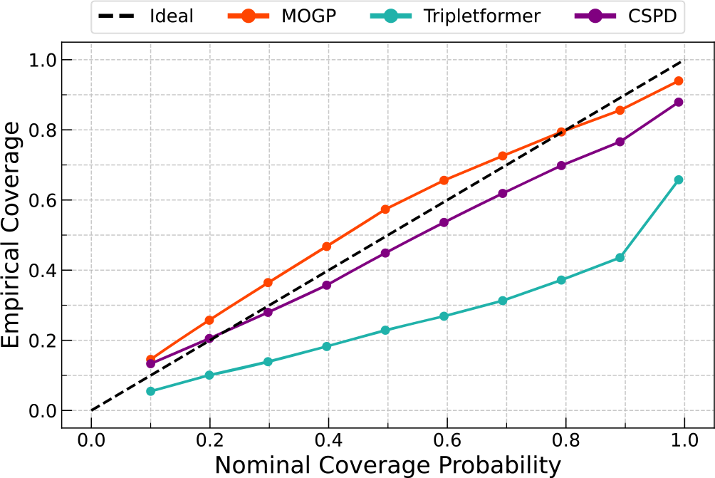
We assessed the calibration of each model’s uncertainty estimates using real Sgr A* observational data. This involved masking random subsets of data to compute the empirical coverage, the fraction of true values falling within the predicted credible intervals, across nominal confidence levels from 10% to 99%). A perfectly calibrated model would align with the identity line, where empirical coverage equals nominal coverage.
As Figure 2 shows, the MOGP consistently demonstrates the best overall calibration, closely tracking the ideal line with slightly conservative uncertainty estimates. The CSPD model also performs well, staying just below the ideal line, indicating a modest underestimation of uncertainty despite its flexibility in learning complex noise structures (e.g., Biloš et al. Reference Biloš, Rasul, Schneider, Nevmyvaka and Günnemann2023). In contrast, the Tripletformer model exhibits significant and consistent undercoverage, meaning it tends to be overconfident in its predictions. This miscalibration likely stems from its simpler, parametric treatment of uncertainty and architectural limitations (e.g., Yalavarthi et al. Reference Yalavarthi, Burchert and Schmidt-Thieme2023).
Coverage analysis of predictive uncertainties across a range of nominal confidence levels, computed on real observational data. Each curve shows the empirical coverage achieved by a model as a function of the nominal coverage level, aggregated across all wavelength bands. The dashed diagonal line indicates perfect calibration. The MOGP (orange) shows the best overall calibration, closely following the ideal line. CSPD (purple) slightly underestimates uncertainty but remains well-calibrated, meanwhile the TripletFormer (teal) consistently undercovers.

5. Future Work
This work demonstrates the promising capability of CSPD for high-fidelity interpolation and uncertainty quantification in sparse, multi-wavelength Sgr A* light curves. This approach significantly enhances our ability to extract information from challenging astrophysical observations.
Moving forward, key areas for improvement include enhancing generalization to real observational data. This involves incorporating more diverse training data, such as a combination of phenomenological and GRMHD-based simulations, and integrating historical observational datasets to account for realistic sampling and noise complexities. Exploring methods like learned observational priors (e.g., Adam et al. Reference Adam, Coogan, Malkin, Legin, Perreault-Levasseur, Hezaveh and Bengio2022) and advanced domain adaptation techniques will also be crucial. Ultimately, these advancements will enable more precise constraints on time delays, significantly advancing our understanding of accreting BHs.


 σ

 Open access

