



%20--%3e%3c!DOCTYPE%20svg%20PUBLIC%20'-//W3C//DTD%20SVG%201.0//EN'%20'http://www.w3.org/TR/2001/REC-SVG-20010904/DTD/svg10.dtd'%3e%3csvg%20version='1.0'%20id='Layer_1'%20xmlns='http://www.w3.org/2000/svg'%20xmlns:xlink='http://www.w3.org/1999/xlink'%20x='0px'%20y='0px'%20width='64px'%20height='64px'%20viewBox='5.5%20-3.5%2064%2064'%20enable-background='new%205.5%20-3.5%2064%2064'%20xml:space='preserve'%3e%3cg%3e%3ccircle%20fill='%23FFFFFF'%20fill-opacity='0'%20cx='37.785'%20cy='28.501'%20r='28.836'/%3e%3cpath%20fill='%23595959'%20d='M37.441-3.5c8.951,0,16.572,3.125,22.857,9.372c3.008,3.009,5.295,6.448,6.857,10.314%20c1.561,3.867,2.344,7.971,2.344,12.314c0,4.381-0.773,8.486-2.314,12.313c-1.543,3.828-3.82,7.21-6.828,10.143%20c-3.123,3.085-6.666,5.448-10.629,7.086c-3.961,1.638-8.057,2.457-12.285,2.457s-8.276-0.808-12.143-2.429%20c-3.866-1.618-7.333-3.961-10.4-7.027c-3.067-3.066-5.4-6.524-7-10.372S5.5,32.767,5.5,28.5c0-4.229,0.809-8.295,2.428-12.2%20c1.619-3.905,3.972-7.4,7.057-10.486C21.08-0.394,28.565-3.5,37.441-3.5z%20M37.557,2.272c-7.314,0-13.467,2.553-18.458,7.657%20c-2.515,2.553-4.448,5.419-5.8,8.6c-1.354,3.181-2.029,6.505-2.029,9.972c0,3.429,0.675,6.734,2.029,9.913%20c1.353,3.183,3.285,6.021,5.8,8.516c2.514,2.496,5.351,4.399,8.515,5.715c3.161,1.314,6.476,1.971,9.943,1.971%20c3.428,0,6.75-0.665,9.973-1.999c3.219-1.335,6.121-3.257,8.713-5.771c4.99-4.876,7.484-10.99,7.484-18.344%20c0-3.543-0.648-6.895-1.943-10.057c-1.293-3.162-3.18-5.98-5.654-8.458C50.984,4.844,44.795,2.272,37.557,2.272z%20M37.156,23.187%20l-4.287,2.229c-0.458-0.951-1.019-1.619-1.685-2c-0.667-0.38-1.286-0.571-1.858-0.571c-2.856,0-4.286,1.885-4.286,5.657%20c0,1.714,0.362,3.084,1.085,4.113c0.724,1.029,1.791,1.544,3.201,1.544c1.867,0,3.181-0.915,3.944-2.743l3.942,2%20c-0.838,1.563-2,2.791-3.486,3.686c-1.484,0.896-3.123,1.343-4.914,1.343c-2.857,0-5.163-0.875-6.915-2.629%20c-1.752-1.752-2.628-4.19-2.628-7.313c0-3.048,0.886-5.466,2.657-7.257c1.771-1.79,4.009-2.686,6.715-2.686%20C32.604,18.558,35.441,20.101,37.156,23.187z%20M55.613,23.187l-4.229,2.229c-0.457-0.951-1.02-1.619-1.686-2%20c-0.668-0.38-1.307-0.571-1.914-0.571c-2.857,0-4.287,1.885-4.287,5.657c0,1.714,0.363,3.084,1.086,4.113%20c0.723,1.029,1.789,1.544,3.201,1.544c1.865,0,3.18-0.915,3.941-2.743l4,2c-0.875,1.563-2.057,2.791-3.541,3.686%20c-1.486,0.896-3.105,1.343-4.857,1.343c-2.896,0-5.209-0.875-6.941-2.629c-1.736-1.752-2.602-4.19-2.602-7.313%20c0-3.048,0.885-5.466,2.658-7.257c1.77-1.79,4.008-2.686,6.713-2.686C51.117,18.558,53.938,20.101,55.613,23.187z'/%3e%3c/g%3e%3c/svg%3e)
%20--%3e%3c!DOCTYPE%20svg%20PUBLIC%20'-//W3C//DTD%20SVG%201.0//EN'%20'http://www.w3.org/TR/2001/REC-SVG-20010904/DTD/svg10.dtd'%3e%3csvg%20version='1.0'%20id='Layer_1'%20xmlns='http://www.w3.org/2000/svg'%20xmlns:xlink='http://www.w3.org/1999/xlink'%20x='0px'%20y='0px'%20width='64px'%20height='64px'%20viewBox='5.5%20-3.5%2064%2064'%20enable-background='new%205.5%20-3.5%2064%2064'%20xml:space='preserve'%3e%3cg%3e%3ccircle%20fill='%23FFFFFF'%20fill-opacity='0'%20cx='37.637'%20cy='28.806'%20r='28.276'/%3e%3cg%3e%3cpath%20fill='%23595959'%20d='M37.443-3.5c8.988,0,16.57,3.085,22.742,9.257C66.393,11.967,69.5,19.548,69.5,28.5c0,8.991-3.049,16.476-9.145,22.456%20C53.879,57.319,46.242,60.5,37.443,60.5c-8.649,0-16.153-3.144-22.514-9.43C8.644,44.784,5.5,37.262,5.5,28.5%20c0-8.761,3.144-16.342,9.429-22.742C21.101-0.415,28.604-3.5,37.443-3.5z%20M37.557,2.272c-7.276,0-13.428,2.553-18.457,7.657%20c-5.22,5.334-7.829,11.525-7.829,18.572c0,7.086,2.59,13.22,7.77,18.398c5.181,5.182,11.352,7.771,18.514,7.771%20c7.123,0,13.334-2.607,18.629-7.828c5.029-4.838,7.543-10.952,7.543-18.343c0-7.276-2.553-13.465-7.656-18.571%20C50.967,4.824,44.795,2.272,37.557,2.272z%20M46.129,20.557v13.085h-3.656v15.542h-9.944V33.643h-3.656V20.557%20c0-0.572,0.2-1.057,0.599-1.457c0.401-0.399,0.887-0.6,1.457-0.6h13.144c0.533,0,1.01,0.2,1.428,0.6%20C45.918,19.5,46.129,19.986,46.129,20.557z%20M33.042,12.329c0-3.008,1.485-4.514,4.458-4.514s4.457,1.504,4.457,4.514%20c0,2.971-1.486,4.457-4.457,4.457S33.042,15.3,33.042,12.329z'/%3e%3c/g%3e%3c/g%3e%3c/svg%3e)
1. Introduction
In recent years, phase-resolved ocean wave models have received increasing attention due to their close relevancy to the safety and efficiency of marine operations. Unlike traditional phase-averaged models (e.g. Booij, Ris & Holthuijsen Reference Booij, Ris and Holthuijsen1999; Tolman et al. Reference Tolman2009), the phase-resolved models aim to predict individual waves, and therefore can capture detailed information of the wave field (usually of  ${O}(1\,\text {km}^2))$ as a guidance for marine operations (e.g. Ma et al. Reference Ma, Sclavounos, Cross-Whiter and Arora2018; Xiao & Pan Reference Xiao and Pan2021). When nonlinear effects are considered, phase-resolved models have been constructed via the high-order spectral (HOS) method (Dommermuth & Yue Reference Dommermuth and Yue1987; West et al. Reference West, Brueckner, Janda, Milder and Milton1987), including its later variants (e.g. Craig & Sulem Reference Craig and Sulem1993; Xu & Guyenne Reference Xu and Guyenne2009), Zakharov equation (Stuhlmeier & Stiassnie Reference Stuhlmeier and Stiassnie2021) and machine learning techniques (Mohaghegh, Murthy & Alam Reference Mohaghegh, Murthy and Alam2021).
In spite of the prosperity of nonlinear wave models, their applications to wave forecast in realistic situations are limited due to the significant uncertainties that grow with time in forecasting chaotic wave motion (e.g. Annenkov & Shrira Reference Annenkov and Shrira2001; Janssen Reference Janssen2008). The source of the uncertainties include (i) the noisy initial conditions of the sea surface, which are usually taken from radar or buoy measurements with certain error characteristics; and (ii) the physical effects, say, of wind and ocean current that are not known a priori and therefore not accurately accounted for in a nonlinear wave model.
In addressing the issues of uncertainty growth, data assimilation (DA) methods have been developed (mostly in the field of geoscience as discussed in Evensen (Reference Evensen2003) and Carrassi et al. (Reference Carrassi, Bocquet, Bertino and Evensen2018)) which combine measurement data and model predictions to improve the analysis of the states. Among the available efforts of applying DA to phase-resolved wave forecast/analysis, most (if not all) focus mainly on addressing the aforementioned uncertainty (i) from initial conditions or measurements, i.e. assuming the prediction model is perfect. These include methods based on variational DA (Aragh & Nwogu Reference Aragh and Nwogu2008; Qi et al. Reference Qi, Wu, Liu, Kim and Yue2018; Fujimoto & Waseda Reference Fujimoto and Waseda2020; Wu, Hao & Shen Reference Wu, Hao and Shen2022) that construct an initial condition to minimize the difference between predictions and measurements in future times, as well as methods based on the Kalman filter (Yoon, Kim & Choi Reference Yoon, Kim and Choi2015) that solve for an optimal wave state at a particular time using prediction and data at the same time. Since the latter methods do not require future data for the analysis, they can be favourably applied in operational wave forecast (as a way to construct an optimal wave state, once data at the same time are available that can be used as initial conditions for the forecast). In this regard, the first and last authors of this paper have developed the EnKF-HOS algorithm (as a substantial extension and improvement to Yoon et al. (Reference Yoon, Kim and Choi2015)) which applies the ensemble Kalman filter (EnKF) coupled with ensemble HOS predictions for analysis and forecast of the ocean wave field.
While the EnKF-HOS method (as the first ensemble-based DA method for phase-resolved ocean waves) has shown remarkable performances in extensive test cases, the uncertainty due to model parameters, i.e. the aforementioned uncertainty source (ii), is not considered except some very heuristic treatment through adaptive inflation (see Wang & Pan (Reference Wang and Pan2021) for details). This is a severe problem for ocean wave forecast as wave evolution can be significantly affected by environmental parameters, e.g. the current and wind fields. One may think of determining these parameters from the global marine weather forecast, but it has to be realized that these global forecast results are usually only available at very coarse grid and sparse time instants. Therefore, a direct interpolation may result in significant errors and will certainly miss the important spatial–temporal variation of these fields on the scales of the wave forecast domain and time horizon, e.g. rogue waves can be triggered as a wave train travels into an opposing current with an increasing current velocity (e.g. Onorato, Proment & Toffoli Reference Onorato, Proment and Toffoli2011; Ducrozet et al. Reference Ducrozet, Abdolahpour, Nelli and Toffoli2021). Another approach is to estimate the current field by fitting a current-modified dispersion relation resolved by the spatial–temporal spectrum of the wave field (Lund et al. Reference Lund, Haus, Horstmann, Graber, Carrasco, Laxague, Novelli, Guigand and Özgökmen2018). However, this method ignores the nonlinearity in the problem and it is also not straightforward to capture the spatial–temporal variation of the current field (which relies on arbitrary placement of windows in time and space). In addition, it requires dense measurements in both space and time which is not practical when only buoy data are available.
In this paper, we continue to develop the EnKF-HOS framework, enabling a simultaneous estimation of the wave states and model parameters. While the developed algorithm can in principle be applied to the estimation of different environmental parameters, we focus here on the ocean current field which can generally vary (slowly) in both space and time. To achieve this goal, we incorporate the current effect on waves to build the HOS-C method, following Wang, Ma & Yan (Reference Wang, Ma and Yan2018) and Pan (Reference Pan2020), as the forward prediction model. When measurements of surface elevation are available, we then solve a DA problem that estimates both the (current) model parameters and (wave) states. We note that this is a non-trivial DA problem since the current parameters form a high-dimensional space (e.g. with the same dimensions as surface elevation in a most general setting) and can only be inferred from their correlation to the wave field (i.e. no direct measurement is available). Upon many trials we adopt an iterative EnKF (IEnKF) (Iglesias, Law & Stuart Reference Iglesias, Law and Stuart2013; Wang & Xiao Reference Wang and Xiao2016) which provides a satisfactory solution to this problem. The developed full method, named IEnKF-HOS-C, is first tested in a series of synthetic problems with various forms (steady/unsteady, uniform/non-uniform) of the current fields. It is shown that the IEnKF-HOS-C method not only provides an accurate estimation of the current field, but also boosts the wave analysis/forecast accuracy even compared to the state-of-the-art EnKF-HOS method. Finally, using real data of surface elevations from a shipborne radar, we show that the IEnKF-HOS-C method successfully recovers the current velocity that matches the in situ measurement by a floating buoy.
The paper is organized as follows. The problem statement and detailed algorithm of the IEnKF-HOS-C method are introduced in § 2. The validation and benchmark of the method against synthetic cases and real marine radar data are presented in § 3. We give a conclusion of the work in § 4.
2. Mathematical formulation and methodology
2.1. Problem statement
We consider the evolution of an ocean wave field under the effect of a surface current  $\boldsymbol {U}(\boldsymbol {x},t)$, which in general can (slowly) vary in both two-dimensional space
 $\boldsymbol {x}$ and time
 $t$. We have available a sequence of measurements of the ocean surface in spatial regions
 $\mathcal {M}_j$, with
 $j=0,1,2,3, \ldots$ being the index of time
 $t$. In general, we allow
 $\mathcal {M}_j$ to be different for different
 $j$, reflecting a mobile system of measurement, e.g. a shipborne marine radar or moving probes. We denote the surface elevation and surface potential (for only waves), reconstructed from the measurements in
 $\mathcal {M}_j$, as
 $\eta _{{m},j}(\boldsymbol {x})$ and
 $\psi _{{m},j}(\boldsymbol {x})$, and assume that the error statistics associated with
 $\eta _{{m},j}(\boldsymbol {x})$ and
 $\psi _{{m},j}(\boldsymbol {x})$ are known a priori from the inherent properties of the measurement equipment.
In addition to the measurements, we have a yet-to-be-developed nonlinear wave model that is able to simulate the evolution of the surface waves (in particular surface elevation  $\eta (\boldsymbol {x},t)$ and wave-only velocity potential
 $\psi (\boldsymbol {x},t)$) under the effect of
 $\boldsymbol {U}(\boldsymbol {x},t)$ given initial conditions. Our purpose is to incorporate measurements
 $\eta _{{m},j}(\boldsymbol {x})$ and
 $\psi _{{m},j}(\boldsymbol {x})$ into the model prediction sequentially (i.e. immediately as data become available in time) to simultaneously construct an optimized analysis of wave states
 $(\eta _{{a},j}(\boldsymbol {x}), \psi _{{a},j}(\boldsymbol {x}))$ and obtain an accurate inference/estimation of
 $\boldsymbol {U}(\boldsymbol {x},t)$.
2.2. The general IEnKF-HOS-C framework
Our new IEnKF-HOS-C method to solve the above problem is built upon the previous EnKF-HOS framework developed in Wang & Pan (Reference Wang and Pan2021). In order to resolve the additional complexities associated with the current field  $\boldsymbol {U}(\boldsymbol {x},t)$, the IEnKF-HOS-C method includes a number of new components (relative to the EnKF-HOS method): (i) a parameter-augmented state space
 $(\eta (\boldsymbol {x},t), \psi (\boldsymbol {x},t), \boldsymbol {U}(\boldsymbol {x},t))$ which includes the current parameters; (ii) the HOS-C method which simulates the evolution of wave field under the effect of
 $\boldsymbol {U}(\boldsymbol {x},t)$, as well as a persistence model (Notton & Voyant Reference Notton and Voyant2018; Wu, Wang & Shadden Reference Wu, Wang and Shadden2019)
 $\partial \boldsymbol {U}(\boldsymbol {x},t)/\partial t=0$, used in the forecast step of the method; and (iii) an iterative procedure in EnKF to build the IEnKF method which successfully handles the high-dimensional state/parameter estimation problem. Figure 1 shows a schematic illustration of the new IEnKF-HOS-C framework. At initial time
 $t=t_0$, measurements
 $\eta _{{m},0}(\boldsymbol {x})$ and
 $\psi _{{m},0}(\boldsymbol {x})$ are available together with an initial guess
 $\boldsymbol {U}_0(\boldsymbol {x})$, based on which we generate ensembles of perturbed (augmented) states
 $(\eta _{{m},0}^{(n)}(\boldsymbol {x}), \psi _{{m},0}^{(n)}(\boldsymbol {x}), \boldsymbol {U}_0^{(n)}(\boldsymbol {x}))$,
 $n=1,2,\ldots,N$, with
 $N$ the ensemble size. A forecast step is then performed, in which an ensemble of
 $N$ HOS-C and persistence-model simulations are conducted, taking
 $(\eta _{{m},0}^{(n)}(\boldsymbol {x}), \psi _{{m},0}^{(n)}(\boldsymbol {x}), \boldsymbol {U}_0^{(n)}(\boldsymbol {x}))$ as initial conditions for each ensemble member
 $n$, until
 $t=t_1$ when the next measurements become available. We note that the persistence model simply states that the forecast
 $\boldsymbol {U}_{{f},1}^{(n)}(\boldsymbol {x})=\boldsymbol {U}_0^{(n)}(\boldsymbol {x})$, but this is not in contradiction to the inference of an unsteady current (see details in § 2.4). At
 $t=t_1$, an analysis step is performed through EnKF where the model forecasts
 $(\eta _{{f},1}^{(n)}(\boldsymbol {x}), \psi _{{f},1}^{(n)}(\boldsymbol {x}),\boldsymbol {U}_{{f},1}^{(n)}(\boldsymbol {x}))$ are combined with new perturbed measurements
 $(\eta _{{m},1}^{(n)}(\boldsymbol {x}), \psi _{{m},1}^{(n)}(\boldsymbol {x}))$ to generate the analysis results
 $(\eta _{{a},1}^{(n)}(\boldsymbol {x}), \psi _{{a},1}^{(n)}(\boldsymbol {x}), \boldsymbol {U}_{{a},1}^{(n)}(\boldsymbol {x}))$. Since
 $\boldsymbol {U}_{{a},1}^{(n)}$ is obtained only through its correlation to the wave field (i.e. no direct measurement) and the forecast step has been possibly performed with an inaccurate current field (i.e.
 $\boldsymbol {U}_0(\boldsymbol {x})\neq \boldsymbol {U}^{{true}}(\boldsymbol {x},t_0)$), it is necessary to conduct iterations between the forecast and analysis steps to facilitate the convergence of the analysed current field to the true situation. In particular, we iterate the forecast and analysis steps every time using the new estimation
 $\boldsymbol {U}_{{a},1}^{(n)}(\boldsymbol {x})$ in analysis to replace
 $\boldsymbol {U}_0^{(n)}(\boldsymbol {x})$ in forecast until a desired tolerance is reached.
Schematic illustration of the IEnKF-HOS-C coupled framework. The size of each ellipse represents the amount of uncertainty.

With  $(\eta _{{a},1}^{(n)}(\boldsymbol {x}), \psi _{{a},1}^{(n)}(\boldsymbol {x}), \boldsymbol {U}_{{a},1}^{(n)}(\boldsymbol {x}))$ available after IEnKF, they are taken as initial conditions for a new ensemble of HOS-C and persistence-model simulations, and the procedures are repeated for
 $t=t_2, t_3, \ldots$ until the desired operation time
 $t_{{max}}$ is reached. We next describe in detail the key components in the IEnKF-HOS-C method, including the generation of measurement ensembles and state augmentation (§ 2.3), the HOS-C method and persistence model (§ 2.4) and the IEnKF procedure (§ 2.5). For simplicity, in the following description we assume that gravitational acceleration and fluid density are unity (so that they do not appear in equations) by choices of proper time and mass units.
2.3. Generation of measurement ensembles and state augmentation
As described in § 2.2, ensembles of perturbed measurements of the surface elevation  $\{ \eta ^{(n)}_{{m},j}(\boldsymbol {x})\}_{n=1}^N$ and velocity potential
 $\{\psi ^{(n)}_{{m},j}(\boldsymbol {x})\}_{n=1}^N$ are needed at both the initialization (
 ${j=0}$) and analysis (
 $j=1,2,3,\ldots$) steps. In addition, an ensemble of initial current velocity
 $\{ \boldsymbol {U}^{(n)}_{0}(\boldsymbol {x})\}_{n=1}^N$ is needed (at
 $t=t_0$) as a state augmentation to start the full IEnKF-HOS-C algorithm.
To illustrate the generation of these ensembles, it is convenient to first define a random field  $w(\boldsymbol {x})$ as a zero-mean Gaussian process with spatial correlation function (Evensen Reference Evensen2003, Reference Evensen2009):
 \begin{equation} C(w(\boldsymbol{x}_1),w(\boldsymbol{x}_2))= \begin{cases} c_w\exp\left(-\displaystyle\frac{|\boldsymbol{x}_1-\boldsymbol{x}_2|^2}{a_w^2}\right), & \text{for}\ |\boldsymbol{x}_1-\boldsymbol{x}_2|\leq\sqrt{3}a_w,\\ 0, & \text{for}\ |\boldsymbol{x}_1-\boldsymbol{x}_2|>\sqrt{3}a_w, \end{cases} \end{equation}
with  $c_w$ the variance of
 $w(\boldsymbol {x})$ and
 $a_w$ the decorrelation length scale.
Following the method proposed by Wang & Pan (Reference Wang and Pan2021), we first produce  $\eta _{{m},j}^{(n)}$ by adding a random-field perturbation
 $w(\boldsymbol {x})$ (defined by (2.1) and with different realizations for different
 $n$) to
 $\eta _{m,j}$, i.e.
 \begin{equation} \eta_{{m},j}^{(n)}(\boldsymbol{x})={\eta}_{{m},j}(\boldsymbol{x})+w(\boldsymbol{x}), \end{equation}
and construct the surface potential  $\psi _{{m},j}^{(n)}$ by linear wave theory:
 \begin{equation} \psi_{{m},j}^{(n)}(\boldsymbol{x})\sim \int\frac{{\rm i}}{ \sqrt{|\boldsymbol{k}|}}\tilde{\eta}_{{m},j}^{(n)}(\boldsymbol{k}) {\rm e}^{{\rm i}\boldsymbol{k}\boldsymbol{{\cdot}}\boldsymbol{x}}\,{\rm d}\boldsymbol{k}, \end{equation}
where  $\tilde {\eta }^{(n)}_{{m},j}(\boldsymbol {k})$ denotes the Fourier coefficient of the
 $n$th member of the perturbed surface elevation at vector wavenumber
 $\boldsymbol {k}$. We note that (2.3) is a direct result of the linear wave equation, and it is not modified by the presence of a uniform current (since physically the current does not affect the velocity field of waves except for a Doppler shift).
To generate the ensemble  $\{ \boldsymbol {U}^{(n)}_{0}(\boldsymbol {x})\}_{n=1}^N\equiv \{ U^{(n)}_{x,0}(\boldsymbol {x}), U^{(n)}_{y,0}(\boldsymbol {x}) \}_{n=1}^N$, we start from an initial guess
 $\boldsymbol {U}_0(\boldsymbol {x}) \equiv (U_{x,0}(\boldsymbol {x}),U_{y,0}(\boldsymbol {x}))$ which is in general not the same as the truth
 $\boldsymbol {U}^{{true}}(\boldsymbol {x},t_0)$. In practice,
 $\boldsymbol {U}_0(\boldsymbol {x})$ can be set as zero or taken from the results of large-scale marine weather forecast. We generate the ensemble of current field by adding another random-field perturbation
 $u(\boldsymbol {x})$ to each component of
 $\boldsymbol {U}_0(\boldsymbol {x})$, i.e.
 \begin{equation} U_{*,0}^{(n)}(\boldsymbol{x})= U_{*,0}(\boldsymbol{x})+u(\boldsymbol{x}), \end{equation}
where the subscript  $*$ represents
 $x$ or
 $y$ and
 $u(\boldsymbol {x})$ is a random field defined by (2.1) with
 $u$ replacing
 $w$, i.e. with variance
 $c_u$ and decorrelation length scale
 $a_u$.
2.4. The HOS-C method and persistence model
Given the initial conditions  $(\eta _{{m},0}^{(n)}(\boldsymbol {x}), \psi _{{m},0}^{(n)}(\boldsymbol {x}), \boldsymbol {U}_0^{(n)}(\boldsymbol {x}))$ or
 $(\eta _{{a},j}^{(n)}(\boldsymbol {x}), \psi _{{a},j}^{(n)}(\boldsymbol {x}), \boldsymbol {U}_{{a},j}^{(n)}(\boldsymbol {x}))$ with
 $j \geq 1$, for each ensemble member
 $n$, the evolution of the (wave and current) augmented state from
 $t_j$ to
 $t_{j+1}$ is solved by integrating a nonlinear wave equation under the effect of the current:
 $$\begin{align} &\frac{\partial\eta(\boldsymbol{x},t)}{\partial t} + \frac{\partial\psi(\boldsymbol{x},t)}{\partial \boldsymbol{x}} \boldsymbol{{\cdot}} \frac{\partial\eta(\boldsymbol{x},t)}{\partial \boldsymbol{x}} -\left[1+\frac{\partial\eta(\boldsymbol{x},t)}{\partial \boldsymbol{x}}\boldsymbol{{\cdot}} \frac{\partial\eta(\boldsymbol{x},t)}{\partial \boldsymbol{x}}\right]\phi_z(\boldsymbol{x},t)\nonumber\\ &\quad +\frac{\partial\eta(\boldsymbol{x},t)}{\partial \boldsymbol{x}}\boldsymbol{{\cdot}} {\boldsymbol{U}}(\boldsymbol{x},t_j)+\eta(\boldsymbol{x},t)\frac{\partial}{\partial \boldsymbol{x}}\boldsymbol{{\cdot}} {\boldsymbol{U}}(\boldsymbol{x},t_j)=0, \end{align}$$
 $$\begin{align} &\frac{\partial\psi(\boldsymbol{x},t)}{\partial t} + \frac{1}{2}\frac{\partial\psi(\boldsymbol{x},t)}{\partial \boldsymbol{x}}\boldsymbol{{\cdot}}\frac{\partial\psi(\boldsymbol{x},t)}{\partial \boldsymbol{x}}+\eta(\boldsymbol{x},t)\nonumber\\ &\quad -\frac{1}{2}\left[1+\frac{\partial\eta(\boldsymbol{x},t)}{\partial \boldsymbol{x}}\boldsymbol{{\cdot}} \frac{\partial\eta(\boldsymbol{x},t)}{\partial \boldsymbol{x}}\right]\phi_z(\boldsymbol{x},t)^2+\frac{\partial\psi(\boldsymbol{x},t)}{\partial \boldsymbol{x}}\boldsymbol{{\cdot}} {\boldsymbol{U}}(\boldsymbol{x},t_j)=0, \end{align}$$
and a persistence model
 \begin{equation} \frac{\partial\boldsymbol{U}(\boldsymbol{x},t)}{\partial t}=0. \end{equation}
In (2.5) and (2.6),  $\phi _z(\boldsymbol {x},t)\equiv \partial \phi /\partial z|_{z=\eta }(\boldsymbol {x},t)$ is the surface vertical velocity with
 $\phi (\boldsymbol {x},z,t)$ being the velocity potential of the wave field, and
 $\psi (\boldsymbol {x},t)\equiv \phi (\boldsymbol {x},\eta,t)$. The variable
 ${\boldsymbol {U}}(\boldsymbol {x},t_j)$ in the equations should be considered as the estimated quantity, taking either
 $\boldsymbol {U}_0^{(n)}(\boldsymbol {x})$ at
 $t=t_0$ or
 $\boldsymbol {U}_{{a},j}^{(n)}(\boldsymbol {x})$ at
 $t=t_j$. Equations (2.5) and (2.6) describe the evolution of a nonlinear wave field under the effect of an irrotational current which slowly varies in space (Wang et al. Reference Wang, Ma and Yan2018; Pan Reference Pan2020). As discussed in Pan (Reference Pan2020), this set of equations form a Hamiltonian system conserving the total energy of the wave and current, and it is possible to relax the scale-separation assumption and irrotational assumption with more developments at certain situations.
The persistence model (2.7) simply states that the current field remains steady in the forecast step, i.e.  $\boldsymbol {U}_{{f},j+1}=\boldsymbol {U}_{{a},j}$ (see applications in other contexts, e.g. Santitissadeekorn & Jones (Reference Santitissadeekorn and Jones2015), Notton & Voyant (Reference Notton and Voyant2018) and Wu et al. (Reference Wu, Wang and Shadden2019)). We remark that this is not in contradiction to the estimation of an unsteady current field which slowly varies in time but can be approximated as a constant in the forecast interval (from
 $t_j$ to
 $t_{j+1}$). In fact, the time variation of the unsteady current is captured in the IEnKF procedure that is discussed in the next section.
2.5. Data assimilation scheme by IEnKF
Let us now assume that we have obtained the forecast ensemble  $\{ \eta ^{(n)}_{{f},j}\}_{n=1}^N$,
 $\{ \psi ^{(n)}_{{f},j}\}_{n=1}^N$ and
 $\{ \boldsymbol {U}^{(n)}_{{f},j}\}_{n=1}^N$ by integrating (2.5)–(2.7) from
 $t_{j-1}$ to
 $t_j$. To describe the analysis step, we first introduce the notation of a covariance operator:
 \begin{equation} \mathfrak{C}(x,y)=\frac{1}{N-1}\sum_{n=1}^N(x^{(n)}-\bar x)(y^{(n)}-\bar y)^{\rm T} \end{equation}
which produces the covariance matrix between two vectors  $x$ and
 $y$ through ensemble average, with the overbar in the equation denoting the ensemble mean.
The analysis step combines  $(\eta ^{(n)}_{{f},j}\in \mathbb {R}^L,\psi ^{(n)}_{{f},j}\in \mathbb {R}^L,\boldsymbol {U}^{(n)}_{{f},j}\in \mathbb {R}^{2L})$ and
 $(\eta ^{(n)}_{{m},j}\in \mathbb {R}^d,\psi ^{(n)}_{{m},j}\in \mathbb {R}^d)$, with
 $L$ and
 $d$ being the dimensions of model (forecast) space and measurement space, respectively. Through EnKF (no iteration yet), this step can be formulated as
 \begin{gather} {\eta^{(n)}_{{a},j}}={\eta^{(n)}_{{f},j}}+{\boldsymbol{Q}_{\eta\eta,j}}{\boldsymbol{G}^\text{T}}(\boldsymbol{G}\boldsymbol{Q}_{\eta\eta,j}\boldsymbol{G}^\text{T}+\boldsymbol{R}_{\eta\eta,j})^{{-}1} ({\eta^{(n)}_{{m},j}}-{\boldsymbol{G}} {\eta^{(n)}_{{f},j}}), \end{gather}
 \begin{gather} {\psi^{(n)}_{{a},j}}={\psi^{(n)}_{{f},j}}+{\boldsymbol{Q}_{\psi\psi,j}}{\boldsymbol{G}^\text{T}}(\boldsymbol{G}\boldsymbol{Q}_{\psi\psi,j}\boldsymbol{G}^\text{T}+\boldsymbol{R}_{\psi\psi,j})^{{-}1} ({\psi^{(n)}_{{m},j}}-{\boldsymbol{G}} {\psi^{(n)}_{{f},j}}), \end{gather}
 \begin{gather} {\boldsymbol{U}^{(n)}_{{a},j}}={\boldsymbol{U}^{(n)}_{{f},j}}+{\boldsymbol{Q}_{U\eta,j}}{\boldsymbol{G}^\text{T}}(\boldsymbol{G}\boldsymbol{Q}_{\eta\eta,j}\boldsymbol{G}^\text{T}+\boldsymbol{R}_{\eta\eta,j})^{{-}1} ({\eta^{(n)}_{{m},j}}-{\boldsymbol{G}} {\eta^{(n)}_{{f},j}}), \end{gather}
where
 \begin{gather} {\boldsymbol{Q}_{xy,j}}=\mathfrak{C}(x_{{f},j}, y_{{f},j}), \end{gather}
 \begin{gather} {\boldsymbol{R}_{xy,j}}=\mathfrak{C}(x_{{m},j}, y_{{m},j}). \end{gather}
The operator (or matrix)  $\boldsymbol {G}:\mathbb {R}^L \rightarrow \mathbb {R}^d$ is an observation operator mapping the
 $L$-dimensional model space to the
 $d$-dimensional measurement space, which is constructed by a linear interpolation in this study (e.g. for measurements on grid points,
 $\boldsymbol {G}$ is reduced to an operation to take the corresponding elements in the model vector). We note that (2.9) and (2.10) are equivalent to the analysis equation (2.13) in Wang & Pan (Reference Wang and Pan2021) written in a form of ensemble matrix. Equation (2.11) provides the update (thus estimation) of the current field, which is achieved through its correlation to the surface elevation field (i.e. the matrix
 $\boldsymbol {Q}_{U\eta,j}$ established through ensembles of HOS-C forecast). In addition, (2.9) and (2.11) combined are equivalent to a standard EnKF equation for an augmented state vector of
 $(\eta,\boldsymbol {U})$. On the other hand, while it is also possible to estimate
 $\boldsymbol {U}$ through its correlation with
 $\psi$, this alternative approach is not more beneficial to (2.11) from both first-principle reasoning and our numerical tests.
Algorithm for the IEnKF-HOS-C method.

Let us next consider the situation that  $\boldsymbol {U}_{{f},j}(\boldsymbol {x})$ is different from the true field
 $\boldsymbol {U}^{{true}}(\boldsymbol {x},t_j)$. While the analysis
 ${\boldsymbol {U}}^{(n)}_{{a},j}(\boldsymbol {x})$ may provide an update that is closer to the truth, the previous forecast step from
 $j-1$ to
 $j$ has been performed with an inaccurate current field. To remedy this situation, it is necessary to perform iterations between the forecast and analysis steps. In particular, for each iteration we replace
 $\boldsymbol {U}^{(n)}_{{a},j-1}(\boldsymbol {x})$ by
 $\boldsymbol {U}^{(n)}_{{a},j}(\boldsymbol {x})$ and repeat the forecast (with updated current field) and analysis steps, until convergence is achieved with a criterion
 \begin{equation} \|\bar{\boldsymbol{U}}_{{f},j}(\boldsymbol{x})-\bar{\boldsymbol{U}}_{{a},j}(\boldsymbol{x})\|_2 < \delta, \end{equation}
or if a preset maximum number of iterations  $h_{{max}}$ is reached. We have now completed the description of the IEnKF-HOS-C method, with a pseudo-code provided in Algorithm 1. In addition, in implementation of IEnKF-HOS-C other practical procedures are required, including the adaptive inflation and localization schemes, and the treatment of the mismatch between the predictable and measurement regions. These procedures are discussed in detail in Wang & Pan (Reference Wang and Pan2021) and are not re-presented in this paper.
3. Results
We validate the IEnKF-HOS-C method through a series of test cases with both synthetic and real ocean wave fields. For each case of the former, a reference HOS-C simulation is conducted with a prescribed current field to produce the true wave solution, onto which random errors are superposed to generate synthetic noisy measurements. For the latter, we make use of the real wave data obtained from an onboard Doppler coherent marine radar (Nwogu & Lyzenga Reference Nwogu and Lyzenga2010; Lyzenga et al. Reference Lyzenga, Nwogu, Beck, O'Brien, Johnson, de Paolo and Terrill2015), with the reference current velocity measured by a floating buoy. For both types of cases, we use  $N=100$ ensemble members in the IEnKF-HOS-C method.
The performance of the IEnKF-HOS-C method can be evaluated by a natural metric of the estimated current field, which should be compared with the reference solutions (prescribed true current fields in the synthetic cases and buoy measurement in the real case). In addition, for the synthetic cases, since the true wave solution is known, another metric can be defined as the error of the analysed wave field relative to the true solution:
 \begin{equation} \epsilon(t)=\frac{\int_\mathcal{A}|\eta^{true}(\boldsymbol{x},t)-\eta^{{sim}}(\boldsymbol{x},t)|^2 \,{\rm d}\mathcal{A}}{2\sigma_{\eta}^2\mathcal{A}}, \end{equation}
where  $\mathcal {A}$ is the area of the simulation region,
 $\sigma ^2_\eta$ is the variance of the reference surface elevation field and
 $\eta ^{{true}}(\boldsymbol {x},t)$ and
 $\eta ^{{sim}}(\boldsymbol {x},t)$ represent, respectively, the true (reference) surface elevation field and the simulation results (that will be obtained through IEnKF-HOS-C, HOS-C-only and our previous EnKF-HOS methods for comparison).
3.1. Synthetic cases
We consider synthetic cases of both two-dimensional (2-D; with one horizontal direction  $x$) and three-dimensional (3-D; with two horizontal directions
 $\boldsymbol {x}=(x,y)$) wave fields. The true wave solution
 $\eta ^{{true}}(\boldsymbol {x},t)$ for each case is generated by a reference HOS-C simulation with an exact initial condition and a prescribed current field. For the 2-D case, we use a reference initial wave field described by a JONSWAP spectrum with a peak wavenumber
 $k_p=16k_0$ (with
 $k_0$ the fundamental wavenumber), a global steepness
 $k_pH_s/2=0.11$ (with
 $H_s$ the significant wave height) and an enhancement factor
 $\gamma =3.3$. For the 3-D case, the initial wave field is taken from the same JONSWAP spectrum peaked at wavenumber
 $k_p=6k_0$, together with a directional spreading function:
 \begin{equation} D(\theta)= \begin{cases} \displaystyle\frac{2}{\beta}\cos^2\left(\displaystyle\frac{\rm \pi}{\beta}\theta \right), & \text{for}\ \displaystyle-\frac{\beta}{2}<\theta<\displaystyle\frac{\beta}{2},\\ 0, & \text{otherwise}, \end{cases} \end{equation}
where  $\beta ={\rm \pi} /6$ is the spreading angle. Without loss of generality, we assume that the true current velocity is always along the
 $x$ direction, expressed as
 \begin{equation} \boldsymbol{U}^{{true}}(\boldsymbol{x})=(U_x^{{true}}(\boldsymbol{x}), U_y^{{true}}(\boldsymbol{x})), \end{equation}
with  $U_y^{{true}}(\boldsymbol {x})=0$ which needs to be estimated together with the non-zero component
 $U_x^{{true}}(\boldsymbol {x})$ in 3-D cases through IEnKF-HOS-C. We remark that in making
 $U_y^{{true}}(\boldsymbol {x})=0$ it is assumed that the incompressibility of the current field, if required, is satisfied through the balance of gradients between
 $x$-direction and vertical motions. This assumption brings conveniences in validating the estimated velocity field, and does not considerably deteriorate the generality of the validation.
To generate the noisy measurements of the wave field, we first superpose a random field onto the reference solution of surface elevation:
 \begin{equation} \eta_{{m}}(\boldsymbol{x})=\eta^{true}(\boldsymbol{x})+w(\boldsymbol{x}), \end{equation}
where  $w(\boldsymbol {x})$ is sampled with
 $c_w=0.0025\sigma ^2_{\eta }$ and
 $a_w={\rm \pi} /2$ in (2.1). Then
 $\psi _{{m}}(\boldsymbol {x})$ is generated based on the linear wave theory (similar to the generation of
 $\psi ^{(n)}_{{m}}(\boldsymbol {x})$ from
 $\eta ^{(n)}_{{m}}(\boldsymbol {x})$ shown in (2.3)):
 \begin{equation} \psi_{{m}}(\boldsymbol{x})\sim\int\frac{{\rm i}}{ \sqrt{|\boldsymbol{k}|}}\tilde{\eta}_{{m}}(\boldsymbol{k}) {\rm e}^{{\rm i}\boldsymbol{k}\boldsymbol{{\cdot}}\boldsymbol{x}}\,{\rm d}\boldsymbol{k}, \end{equation}
where  $\tilde {\eta }_{{m}}(\boldsymbol {k})$ denotes the measured surface elevation in Fourier space. Regarding the initial guess of current velocity
 ${U}_{*,0}$, we assume it to be uniform, and reasonable to some extent (with its deviation from
 $U_*^{{true}}$ not too large) due to the existence of marine weather forecast information or other approaches to roughly estimate a constant current field from radar data (e.g. Lund et al. Reference Lund, Haus, Horstmann, Graber, Carrasco, Laxague, Novelli, Guigand and Özgökmen2018) in practice. Cases with zero initial current velocity will also be tested.
Finally, on the computation side, we use  $L=256$ grid points with a spatial domain
 $\mathcal {A}=[0,2{\rm \pi} )$ for 2-D simulations and
 $L=64\times 64$ grid points with
 $\mathcal {A}=[0,2{\rm \pi} )\times [0,2{\rm \pi} )$ for 3-D simulations. We next describe all synthetic cases classified by the form of the current fields that can be uniform/non-uniform and steady/unsteady.
3.1.1. Results for uniform current fields
We start from relatively simple cases with a uniform current field that can be steady or unsteady. Under this situation, the current field to be estimated at each time instant is reduced to a scalar for the 2-D cases or a vector with two components for the 3-D cases. In the analysis step, (2.11) can be modified accordingly in dimensions for the simplified scalar (vector) velocity fields.
Steady cases
We consider both 2-D and 3-D wave fields with the true current velocity given by
 \begin{equation} U_x^{{true}}={0.025}v_p(k_p), \end{equation}
where  $v_p(k_p)$ represents the phase velocity of the peak wavenumber
 $k_p$ in the JONSWAP spectrum. The initial guess of the current velocity is predefined as
 \begin{equation} {U}_{x,0}={0.03}v_p(k_p) \end{equation}
for the 2-D case and
 \begin{equation} \boldsymbol{U}_{0}=({0.03}v_p(k_p),{0.005}v_p(k_p)) \end{equation}
for the 3-D case. We note that a non-zero  $y$ component is used for
 $\boldsymbol {U}_{0}$ even though the truth is zero. The ensemble of the current velocity is generated by superposing zero-mean random errors, which are sampled from (2.1) with
 $c_u=0.04(U_x^{{true}})^2$ and
 $a_u \rightarrow \infty$, onto each component of the initial guess.
For the IEnKF-HOS-C simulations, data from  $d=12$ locations (randomly selected with a uniform distribution) are assimilated with an interval
 $\tau =T_p/32$, with
 $T_p$ the wave period for the peak mode
 $k_p$. The simulations start from the noisy measurements of the initial wave field (which are generated by (3.4) and (3.5)) and the initial guess of the current velocity, and are conducted until
 $t=100T_p$.
The errors  $\epsilon (t)$ obtained from IEnKF-HOS-C and HOS-C-only simulations (starting from the same wave field and initial guess of current velocity) are shown in figure 2. For both 2-D and 3-D cases, as the simulation proceeds
 $\epsilon (t)$ obtained from the HOS-C-only method increases from the initial value
 $\epsilon (0)\approx 0.05$ and approaches
 ${O}(1)$ at
 $t/T_p\approx 100$; whereas with the IEnKF-HOS-C method,
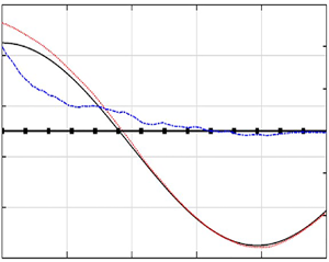
 $\epsilon (t)$ keeps decreasing as the measurements are assimilated sequentially, and becomes two orders of magnitude smaller than its initial value at the end of the simulations. To further visualize the wave fields, figures 3 and 4 show snapshots of
 $\eta ^{{true}}(x)$ and
 $\eta ^{{sim}}(x)$ obtained from both IEnKF-HOS-C and HOS-C-only methods at three time instants of
 $t/T_p=10$,
 $50$ and
 $90$ for the 2-D and 3-D cases, respectively. It can be found that, for both cases,
 $\eta ^{{sim}}(x)$ from the IEnKF-HOS-C method exhibits a much better agreement with
 $\eta ^{{true}}(x)$ than that from the HOS-C-only method. At
 $t/T_p=90$, the IEnKF-HOS-C solution is already almost indistinguishable from
 $\eta ^{true}(x)$.
Errors  $\epsilon (t)$ from IEnKF-HOS-C (red dotted line) and HOS-C-only (black solid line) methods, for (a) 2-D and (b) 3-D cases with a steady and uniform current field.

Surface elevations  $\eta ^{{true}}(x)$ (blue dash-dotted line),
 $\eta ^{{sim}}(x)$ with IEnKF-HOS-C (red dotted line) and HOS-C-only (black solid line) methods, at (a)
 $t/T_p=10$, (b)
 $t/T_p=50$ and (c)
 $t/T_p=90$, for the 2-D wave field.

Surface elevations  $\eta ^{{true}}(x)$ (blue dash-dotted line),
 $\eta ^{{sim}}(x)$ with IEnKF-HOS-C (red dotted line) and HOS-C-only (black solid line) methods for the cross-section
 $y/2{\rm \pi} =0.3$ in the 3-D wave field, at (a)
 $t/T_p=10$, (b)
 $t/T_p=50$ and (c)
 $t/T_p=90$.

Another important metric for evaluating the IEnKF-HOS-C performance is the estimated current velocity  $\boldsymbol {U}_{a}$, which is shown in figure 5 together with
 $\boldsymbol {U}^{{true}}$ for both 2-D and 3-D cases. It can be found that, as the measurements of the surface elevation are assimilated,
 $\boldsymbol {U}^{a}$ approaches
 $\boldsymbol {U}^{true}$ (although experiencing some fluctuations) with their difference practically negligible after
 $t/T_p=40$. This indicates that the IEnKF-HOS-C algorithm is successful in the estimation of current velocity in these cases.
Current velocity  $\boldsymbol {U}_{{a}}$ estimated by the IEnKF-HOS-C method (
 ${U}_{x,{a}}$, red dotted line;
 ${U}_{y,{a}}$, blue dash-dotted line), in comparison with the true values (black solid line), for (a) 2-D and (b) 3-D cases with a steady and uniform current field. In (b) the
 $y$ component of the velocity is labelled on the right-hand vertical axis.

We further test the performance of the IEnKF-HOS-C method when initial guess of zero-velocity current field is used. Although in practice better initial guesses are usually available, this test provides a challenging case with large deviation of initial guess from the true current field. The error  $\epsilon (t)$ and estimated current velocity
 $\boldsymbol {U}^{a}$ are shown in figures 6 and 7, respectively. From figure 7 we see that it takes
 ${O}(60T_p)$ for the estimated velocity to converge to the true values, which is slower than the cases with initial guesses (3.7) and (3.8) shown in figure 5. This is also reflected in figure 6 where the error with zero initial guess drops slower than that with (3.7) and (3.8). However, it is also clear in figure 6 that the former drops with a rate that is comparable to or faster than the latter for
 $t>{O}(60T_p)$ since the correct current velocity has been captured by the former. In addition, we also include in figure 6 the result of the previous EnKF-HOS method developed by Wang & Pan (Reference Wang and Pan2021), which characterizes the situation of a biased physical model coupled with DA (that can partially correct the solution). We observe that
 $\epsilon (t)$ from EnKF-HOS decreases in time with a much slower rate than the two results from IEnKF-HOS-C, with the error from IEnKF-HOS-C up to one order of magnitude smaller than that from EnKF-HOS at
 $t=100T_p$.
Errors  $\epsilon (t)$ from IEnKF-HOS-C (with initial guess of current velocity given by (3.7) or (3.8): red dotted line; with zero initial guess of current velocity: blue dashed line) and EnKF-HOS (magenta solid line) methods, for (a) 2-D and (b) 3-D cases with a steady and uniform current field.

Current velocity  $\boldsymbol {U}_{{a}}$ estimated by the IEnKF-HOS-C method (
 ${U}_{x,{a}}$, red dotted line;
 ${U}_{y,{a}}$, blue dash-dotted line), in comparison with the true values (black solid line), for (a) 2-D and (b) 3-D cases with a steady and uniform current field. In (b) the
 $y$ component of the velocity is labelled on the right-hand vertical axis.

Finally, we test the robustness of the IEnKF-HOS-C method for opposing current, by reversing the signs in (3.6), (3.7) and (3.8), and keeping the initial wave states the same as before. Results shown in figures 8 and 9 demonstrate the performance of IEnKF-HOS-C to effectively estimate the opposing current field together with improved accuracy in wave-field reconstruction. The current estimation now takes  ${O}(60T_p)$ to converge to the true values (seemingly longer than the following current case) mainly because the opposing current effect slows down the wave propagation, which makes the time to convergence longer when normalized by the intrinsic period
 $T_p$.
Errors  $\epsilon (t)$ from IEnKF-HOS-C (red dotted line) and HOS-C-only (black solid line) methods, for (a) 2-D and (b) 3-D cases with opposing current fields.

Current velocity  $\boldsymbol {U}_{{a}}$ estimated by the IEnKF-HOS-C method (
 ${U}_{x,{a}}$, red dotted line;
 ${U}_{y,{a}}$, blue dash-dotted line), in comparison with the true values (black solid line), for (a) 2-D and (b) 3-D cases with opposing current fields. In (b) the
 $y$ component of the velocity is labelled on the right-hand vertical axis.

Unsteady cases
In this section, we test the performance of the IEnKF-HOS-C method for unsteady and uniform current fields. We focus on 3-D wave fields hereafter and for this section we consider both linear and sinusoidal time variations of the current fields, described by
 \begin{equation} U_x^{{true}}(t)=(1+\alpha_1 t/T_p)U_c \end{equation}
and
 \begin{equation} U_x^{{true}}(t)=(\cos(\alpha_2 t/T_p)+1.12)U_c, \end{equation}
with  $\alpha _1=0.005$,
 $\alpha _2=0.04$ and
 $U_c=0.025v_p(k_p)$. The initial guess of current velocity is also prescribed by (3.8), based on which the ensemble is then produced with
 $c_u=0.04(U_c)^2$ and
 $a_u \rightarrow \infty$. Noisy measurements of the wave field at
 $24$ randomly sampled locations are assimilated with an interval
 $\tau =T_p/32$.
Figure 10 shows the errors  $\epsilon (t)$ from the IEnKF-HOS-C and HOS-C-only methods, for the two current fields (3.9) and (3.10). For the HOS-C-only simulations,
 $\epsilon (t)$ grows quickly in time (somewhat faster than for the steady current cases at the early stage of simulations) and reaches
 ${O}(1)$ at
 $t/T_p \approx 80$. The IEnKF-HOS-C method is again successful in accurately estimating the wave fields with the error
 $\epsilon (t)$ reducing to
 ${O}(10^{-3})$ at
 $t/T_p \approx 100$.


Figure 11 presents the estimated velocity by the IEnKF-HOS-C method, in terms of its evolution in time and comparison to the true current velocity  $\boldsymbol {U}^{{true}}(t)$. For both types of current fields (3.9) and (3.10), the IEnKF-HOS-C method is able to track the variation of the current field, with
 $\boldsymbol {U}_{{a},j}$ converging to the vicinity of the true time series after
 $40T_p$–
 $60 T_p$. We remark that the capability to capture the unsteadiness of the current is achieved through the IEnKF procedure, in spite of the persistence model (2.7) in the forecast step.
Estimations  $\boldsymbol {U}_{{a},j}$ from the IEnKF-HOS-C method (
 $U_{x,{a}}$, red dotted line;
 $U_{y,{a}},$ blue dash-dotted line), in comparison with the true values (
 $U_{x}^{{true}}(t)$, black solid line;
 $U_{y}^{{true}}(t)=0$, line with squares), for the cases with unsteady and uniform current fields: (a) (3.9) and (b) (3.10).

3.1.2. Results for non-uniform current fields
We further demonstrate the effectiveness of the IEnKF-HOS-C method for the 3-D wave-field evolution under the effect of non-uniform current fields. The results below are presented for steady and unsteady non-uniform current fields.
Steady case
We consider the wave-field evolution under the effect of a steady and non-uniform (varying in  $x$ direction) current field, which is described by
 \begin{equation} U^{{true}}_x(x)= \begin{cases} \displaystyle\frac{U_1+{\rm e}^{\gamma x-q}U_2}{{\rm e}^{\gamma x-q}+1}, & \text{for}\ \displaystyle0\leq x\leq {\rm \pi},\\ U_x^{{true}}(2{\rm \pi}-x), & \text{for}\ \displaystyle {\rm \pi}< x\leq 2{\rm \pi} \end{cases} \end{equation}
and plotted in figure 12. The parameter values are chosen as  $U_1=0.01v_p(k_p)$,
 $U_2=0.025v_p(k_p)$,
 $q=15$ and
 $\gamma ={25}/{{\rm \pi} }$ such that the transitions between the locally uniform regions are smooth (i.e. slow variation of the current field compared with the wave oscillation, and thus compatible with (2.5) and (2.6)).
Plot of  $U_x^{{true}}(x)$ as the true steady and non-uniform current field described by (3.11).

In this case, we set the initial guess of current velocity to be uniform as before (assuming no spatial distribution information is accessible a priori):
 \begin{gather} U_{x,0}(\boldsymbol{x})=0.15v_p(k_p), \end{gather}
 \begin{gather} U_{y,0}(\boldsymbol{x})=0.02v_p({k}_p), \end{gather}
with the initial ensemble for both velocity components generated by (2.4) with  $c_u=0.04(U_1)^2$ and
 $a_u={\rm \pi} /2$.
With the IEnKF-HOS-C method, data of surface elevation at  $d=64$ randomly selected locations are assimilated into the numerical model with an interval
 $\tau =T_p/64$. Figure 13 plots the errors
 $\epsilon (t)$ obtained from the IEnKF-HOS-C and HOS-C-only methods for this case, showing again that IEnKF-HOS-C is successful in estimating the wave states, in contrast to the HOS-C-only simulation.
Errors  $\epsilon (t)$ from the IEnKF-HOS-C (red dotted line) and HOS-C-only (black solid line) methods for the current field described by (3.11).

The current fields captured by IEnKF-HOS-C, in terms of the snapshots of  $U_{x,{a}}(\boldsymbol {x})$ and
 $U_{y,{a}}(\boldsymbol {x})$ at three cross-sections of constant
 $y$ for
 $t/T_p=10$,
 $50$ and
 $90$, are plotted in figure 14. We see that the estimated velocity starts from a constant value and converges to the true field (with its variation in
 $x$ captured at all cross-sections) as the time increases. This successful estimation of the current field is the basis for the accurate prediction of the wave states seen in figure 13.
Estimations  $U_{x,{a}}$ (a,c,e) and
 $U_{y,{a}}$ (b,d, f) by IEnKF-HOS-C at (a,b)
 $t/T_p=10$, (c,d)
 $t/T_p=50$ and (e, f)
 $t/T_p=90$ in comparison with the true current field (3.11) (black solid line), for three cross-sections:
 $y/2{\rm \pi} =0.25$ (red dotted line),
 $y/2{\rm \pi} =0.50$ (blue dash-dotted line) and
 $y/2{\rm \pi} =0.75$ (magenta dashed line).

Unsteady cases
The climax of the synthetic cases is the application of the IEnKF-HOS-C method to the wave-field evolution impacted by a current field featuring both spatial and temporal variations. In particular, we assign a sinusoidal variation to the current field (3.11) to produce the true current velocity field:
 \begin{equation} U^{{true}}_x(\boldsymbol{x},t)= \begin{cases} \displaystyle\frac{U_1+{\rm e}^{\gamma x-q}U_2}{{\rm e}^{\gamma x-q}+1}\cos(\alpha_3 t/T_p), & \text{for}\ \displaystyle0\leq x\leq {\rm \pi},\\ U_x^{{true}}(2{\rm \pi}-x), & \text{for}\ \displaystyle {\rm \pi}< x\leq 2{\rm \pi}, \end{cases} \end{equation}
where  $\alpha _3=0.01$. For this case we use the same initial guess of current velocity as in the steady case, i.e. (3.12) and (3.13), as well as the same corresponding initial ensembles generated by (2.4) with
 $c_u=0.04(U_1)^2$ and
 $a_u={\rm \pi} /2$.
The time series of  $\epsilon (t)$ from the IEnKF-HOS-C and HOS-C-only methods are shown in figure 15, which demonstrates, similar to all above cases, the effectiveness of IEnKF-HOS-C in reproducing the wave states. The estimated current field by IEnKF-HOS-C is further plotted in figure 16, in terms of the snapshots of
 $U_{x,{a}}$ and
 $U_{y,{a}}$ at the three cross-sections of constant
 $y$ for three time instants
 $t/T_p=10$,
 $50$ and
 $90$. Starting from an initial guess of a constant field,
 $U_{x,{a}}$ captures both the spatial and temporal variation of
 $U^{{true}}_x(\boldsymbol {x},t)$ and
 $U_{y,{a}}$ approaches zero uniformly in time with sequential data assimilated to the algorithm.
Error  $\epsilon (t)$ from the IEnKF-HOS-C (red dotted line) and HOS-C-only (black solid line) methods for the current field described by (3.14).

Estimations  $U_{x,{a}}$ (a,c,e) and
 $U_{y,{a}}$ (b,d, f) by IEnKF-HOS-C at (a,b)
 $t/T_p=10$, (c,d)
 $t/T_p=50$ and (e, f)
 $t/T_p=90$ in comparison with the true field (3.14) (black solid line), for three cross-sections:
 $y/2{\rm \pi} =0.25$ (red dotted line),
 $y/2{\rm \pi} =0.50$ (blue dash-dotted line) and
 $y/2{\rm \pi} =0.75$ (magenta dashed line).

3.2. The case with real wave data
In what follows, we test the IEnKF-HOS-C method using real measurements of the ocean wave field presented in Lyzenga et al. (Reference Lyzenga, Nwogu, Beck, O'Brien, Johnson, de Paolo and Terrill2015). The measurements are obtained from an onboard  $25\,\text {kW}$ X-band (
 $9.4\,\text {GHz}$) Doppler coherent marine radar off the coast of southern California. A patch of the radar-scanned area, which is fixed in the local radar coordinate system and covers a
 $480\,{\rm m}\times 480\,{\rm m}$ region, is selected as the domain of interest. The numerical simulation starts from 23:18:32 UTC on 17 September 2013 and lasts for
 $40T_p$ with
 $T_p=11.28\,\text {s}$. The initial condition is taken from the measurements in the computational domain (figure 17) featuring a global wave steepness
 $k_pH_s/2=0.02$. In figure 17 it can be clearly observed that the dominant wavelength is
 $\lambda _p\approx 200\,\text {m}$ that is consistent with the estimated value by the linear wave theory for
 $T_p=11.28\,\text {s}$. We use
 $L=64\times 64$ grid points in the simulation, which matches the resolution in the radar dataset. The DA interval is set to be the same as the data acquisition interval of the radar, which fluctuates around
 $T_p/4=2.82\,\text {s}$, i.e. after each interval we assimilate radar data into the IEnKF-HOS-C simulation.
Initial surface elevation  $\eta _{m,0}(\boldsymbol {x})/H_s$ (with
 $H_s=1.50\,\text {m}$) measured by radar at
 $t=t_0$, i.e. 23:18:32 UTC on 17 September 2013.

The reference velocity of the current field in this case is taken from the track of an in situ floating buoy from 23:10:10 to 23:25:02 UTC on 17 September 2013, which is shown in figure 18. While it is preferable to obtain the spatial and temporal variations of the current field, the available information only allows us to compute the mean velocity of the floating buoy, as  $\boldsymbol {U}_b=(0.2958,-0.3944)\,{\rm m}\,{\rm s}^{-1}$. On the other hand, due to the relatively small size of the simulation domain and short time interval, it can be justified to consider a uniform and steady current field with velocity specified by
 $\boldsymbol {U}_b$.
Ship and buoy tracks for the time interval from 23:10:10 to 23:25:02 UTC on 17 September 2013 (Lyzenga et al. Reference Lyzenga, Nwogu, Beck, O'Brien, Johnson, de Paolo and Terrill2015). The initial simulation domain at  $t_0=23$:18:32 is marked as the grey square box.

To generate ensemble of measurements of the wave field, we use (2.2) and (2.3) with  $c_w=0.0025\sigma _{\eta }^2$ and
 $a_w=120\,\text {m}$ defined in (2.1). Four different initial guesses of the current velocity are considered, namely
 $\boldsymbol {U}_0=(0.1958,-0.4944)$,
 $\boldsymbol {U}_0=(0.3958, -0.2944)$,
 $\boldsymbol {U}_0=(0.3958, -0.4944)$ and
 $\boldsymbol {U}_0=(0.1958, -0.2944)$, all representing a shift of
 $0.1\,{\rm m}\,{\rm s}^{-1}$ in different directions of each component of
 $\boldsymbol {U}_b$. The ensemble of the initial current velocity is generated by (2.4) with
 $c_u=0.02\,\text {m}^2\,\text {s}^{-2}$ and
 $a_u=120\,\text {m}$.
An issue that needs to be considered for such a realistic case with uncertain boundary conditions is the problem of predictable zone and its potential mismatch with the measurement region. This issue has been discussed in detail in Wang & Pan (Reference Wang and Pan2021), which involves the application of a modified analysis equation in EnKF (IEnKF in this case). For conciseness, we do not present the details again in this paper but refer the interested readers to our previous paper (Wang & Pan Reference Wang and Pan2021). These previously developed techniques are also applied here, with the only additional complexity that the estimated current velocity  $\boldsymbol {U}_{{a},j}$ now needs to be added to the wave group velocity (accounting for the Doppler shift) to determine the boundaries of the predictable zones.
Figure 19 presents the estimation  $U_{x,{a}}$ and
 $U_{y,{a}}$, in comparison with the reference velocity
 $\boldsymbol {U}_b$, obtained with different initial guesses. For all the initial guesses, we see that the estimation
 $\boldsymbol {U}_{{a},j}$ converges to the reference
 $\boldsymbol {U}_b$ at
 $t_j\approx 40T_p$. In order to assess the performance of IEnKF-HOS-C in terms of the wave-field reconstruction, we use the following two metrics (since the true wave states are inaccessible and (3.1) is not defined):
 \begin{gather} {\rho(\eta_{{m},j},\eta^{sim})=\frac{\int_\mathcal{A}\eta_{{m}, j}(\boldsymbol{x})\eta^{sim}(\boldsymbol{x}) \,{\rm d}\mathcal{A}}{\sigma_{\eta}^2 \mathcal{A}},} \end{gather}
 \begin{gather} {\mathcal{D}=\frac{\rm{tr}\left(\mathfrak{C}\left(\eta_{{a}}, \eta_{{a}}\right)\right)}{L},} \end{gather}
where  $\rm {tr}(\varLambda )$ represents the trace of a matrix
 $\varLambda$. The correlation coefficient
 $\rho (\eta _{{m},j},\eta ^{{sim}})$ provides a measure of the difference between measurements and simulation results, which is also an indication of the magnitude of the correction (innovation) terms in (2.9)–(2.11). The quantity
 $\mathcal {D}$ provides the ensemble variance of the analysis field
 $\eta _{a}$ averaged over space (see (2.8) for the definition of operator
 $\mathfrak {C}$, and
 $L$ is the total number of grid points), which measures the uncertainty level after each analysis step in the simulation. For a simulation with better DA reconstruction of the wave field, it is expected that
 $\rho$ and
 $\mathcal {D}$ are respectively higher and lower. This is indeed the case as we observe in figures 20 and 21, which show the time series of
 $\rho$ and
 $\mathcal {D}$ respectively obtained from the IEnKF-HOS-C and EnKF-HOS methods. It is clear that IEnKF-HOS-C provides better results in terms of measures by both quantities. In addition, we see that the reconstruction quality of IEnKF-HOS-C gradually increases with time after
 $t/T_p =15$–
 $20$, which is mainly due to the improved estimation of current with time. The above results clearly demonstrate the effectiveness of IEnKF-HOS-C when applied to real radar data, although tests against more sophisticated cases are warranted for future studies (which require better and detailed measurements of the ocean current field together with remote sensing of the surface waves).
Estimations  $U_{x, {a}}$ (red dotted line, left-hand axis) and
 $U_{y, {a}}$ (blue dash-dotted line, right-hand axis) by IEnKF-HOS-C, in comparison with the reference velocity
 $\boldsymbol {U}_b$ (black solid line), for four different initial guesses of the current velocity: (a)
 $\boldsymbol {U}_0=(0.1958,-0.4944)\,{\rm m}\,{\rm s}^{-1}$; (b)
 $\boldsymbol {U}_0=(0.3958, -0.2944)\,{\rm m}\,{\rm s}^{-1}$; (c)
 $\boldsymbol {U}_0=(0.3958, -0.4944)\,{\rm m}\,{\rm s}^{-1}$; and (d)
 $\boldsymbol {U}_0=(0.1958, -0.2944)\,{\rm m}\,{\rm s}^{-1}$.

Time series of  $\rho (\eta _{{m},j},\eta ^{{sim}})$ from IEnKF-HOS-C (with
 $\boldsymbol {U}_0=(0.1958,-0.4944)$, red dotted line;
 $\boldsymbol {U}_0=(0.3958, -0.2944)$, blue dash-dotted line;
 $\boldsymbol {U}_0=(0.3958, -0.4944)$, magenta dashed line;
 $\boldsymbol {U}_0=(0.1958, -0.2944)$, cyan line with circles) and EnKF-HOS (black solid line) methods.

Time series of  $\mathcal {D}$ from IEnKF-HOS-C (with
 $\boldsymbol {U}_0=(0.1958,-0.4944)$, red dotted line;
 $\boldsymbol {U}_0=(0.3958, -0.2944)$, blue dash-dotted line;
 $\boldsymbol {U}_0=(0.3958, -0.4944)$:, magenta dashed line;
 $\boldsymbol {U}_0=(0.1958, -0.2944)$, cyan line with circles) and EnKF-HOS (black solid line) methods.

We finally test the robustness of the developed IEnKF-HOS-C algorithm by switching the simulation initialization time  $t_0$, with the simulation period remaining at
 $40T_p$. Specifically, three additional choices of
 $t_0$ between 23:10:10 and 23:25:02 UTC on 17 September 2013 are tested, namely 23:12:03, 23:14:22 and 23:16:28, for the case with
 $\boldsymbol {U}_0=(0.3958, -0.4944)\,{\rm m}\,{\rm s}^{-1}$. Figure 22 presents the estimated current velocity
 $\boldsymbol {U}_{{a}}$ for four different choices of
 $t_0$. It can be found that the estimated velocity at
 $40T_p$ indeed varies to some extent, but all within
 $O(10\,\%)$ difference compared with the buoy measurement. This further demonstrates the robustness of the IEnKF-HOS-C algorithm, considering many factors that can cause the difference in estimated velocity in different windows, e.g. the (unknown) fluctuation of the true velocity in time and space.
Estimations (a)  $U_{x, {a}}$ and (b)
 $U_{y, {a}}$ by IEnKF-HOS-C for
 $t_0=23$:12:03 (magenta dashed line),
 $t_0=23$:14:22 (cyan line with circles),
 $t_0=23$:16:28 (blue dash-dotted line) and
 $t_0=23$:18:32 (red dotted line), in comparison with
 $\boldsymbol {U}_b$ (black solid line).

4. Conclusions
In this paper, we present a new IEnKF-HOS-C method, which features the capability of simultaneous phase-resolved ocean wave forecast and current estimation. The performance of the IEnKF-HOS-C method is examined using both synthetic data and measurements in the real ocean environment. As indicated by the numerical results, the developed IEnKF-HOS-C method outperforms not only the HOS-C-only method but also the state-of-the-art EnKF-HOS method, in terms of the wave forecast accuracy. In addition, the feasibility of inferring current velocity with this method is extensively demonstrated, by testing it for various forms of current fields, which are characterized by distinct temporal and spatial variations. The developed IEnKF-HOS-C method is intrinsically extensible and can be easily modified to account for other physical or empirical parameters. Finally, if implemented on a graphics processing unit, this method can be conveniently carried out in offshore environments, which may bring in favourable effects in marine operations.
Acknowledgement
The authors would like to thank Dr D. Lyzenga in the Department of Naval Architecture and Marine Engineering at the University of Michigan for providing and interpreting the radar data.
Funding
G.W., J.Z., Q.Z. and Z.L. acknowledge funding from the National Key Research and Development Program of China (2021YFB2601100). G.W., J.Z., Y.M. and Z.L. acknowledge funding from the Open Funds of State Key Laboratory of Coastal and Offshore Engineering of China (Project No. LP2101).
Declaration of interests
The authors report no conflict of interest.


 Open access

