1 Introduction
Fluid deformable surfaces are a common motif in cell and tissue biology. For instance, lipid bilayers are fluid thin sheets that define the boundary of cells and compartmentalize them. They are the base material for the plasma membrane, the endoplasmic reticulum, mitochondria or the Golgi apparatus. From a mechanical viewpoint, lipid bilayers are remarkably soft materials exhibiting a solid–fluid duality: while they store elastic energy when stretched or bent, as solid shells (Lipowsky Reference Lipowsky1991), they cannot store elastic energy under in-plane shear, a situation under which they flow as viscous two-dimensional fluids (Dimova et al. Reference Dimova, Aranda, Bezlyepkina, Nikolov, Riske and Lipowsky2006). This solid–fluid duality is tightly intertwined with membrane geometry: shape changes induce lipid flows that bring material from one part of the membrane to another (Evans & Yeung Reference Evans and Yeung1994), whereas flows in the presence of curvature generate out-of-plane forces, which further curve the membrane (Rahimi, DeSimone & Arroyo Reference Rahimi, DeSimone and Arroyo2013). The solid–fluid duality of membranes is essential for cell function; it is required during cell motility and migration (Arroyo et al. Reference Arroyo, Heltai, Millán and DeSimone2012; Lieber et al. Reference Lieber, Schweitzer, Kozlov and Keren2015), membrane trafficking (Sprong, van der Sluijs & van Meer Reference Sprong, van der Sluijs and van Meer2001; Rustom et al. Reference Rustom, Saffrich, Markovic, Walther and Gerdes2004) or to enable the mechano-adaptation of cells to stress (Staykova et al. Reference Staykova, Arroyo, Rahimi and Stone2013; Kosmalska et al. Reference Kosmalska, Casares, Elosegui-Artola, Thottacherry, Moreno-Vicente, González-Tarragó, del Pozo, Mayor, Arroyo and Navajas2015). Furthermore, the in-plane fluidity of the membrane allows membrane inclusions, such as proteins, to diffuse (Saffman & Delbrück Reference Saffman and Delbrück1975; Sens, Johannes & Bassereau Reference Sens, Johannes and Bassereau2008). On the other hand, lipid bilayers are chemically responsive. Chemo-mechanical couplings can trigger tubulation (Roux et al. Reference Roux, Cappello, Cartaud, Prost, Goud and Bassereau2002), phase separation (Bacia, Schwille & Kurzchalia Reference Bacia, Schwille and Kurzchalia2005), budding and fission (Staneva, Angelova & Koumanov Reference Staneva, Angelova and Koumanov2004; Zhou & Yan Reference Zhou and Yan2005) or pearling (Khalifat et al. Reference Khalifat, Rahimi, Bitbol, Seigneuret, Fournier, Puff, Arroyo and Angelova2014).
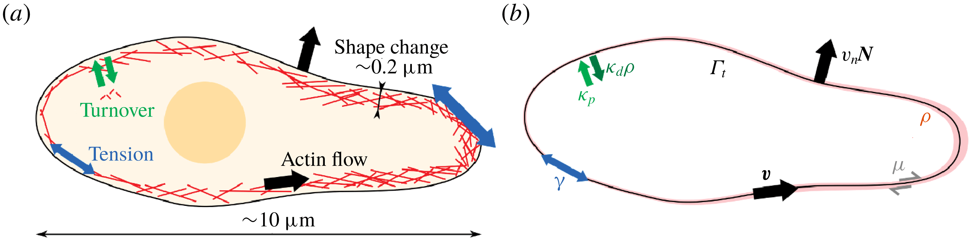
Another important instance of biological fluid surface is the actomyosin cortex, a thin network of cross-linked actin filaments lying immediately beneath the plasma membrane of animal cells (Bray & White Reference Bray and White1988). Within this network, myosin motors exert active forces by consuming chemical energy in the form of adenosine triphosphate (ATP), that generate active tension (Salbreux, Charras & Paluch Reference Salbreux, Charras and Paluch2012). Furthermore, the cell cortex undergoes dynamic remodelling, or turnover, in less than one minute, as a result of the polymerization and depolymerization of actin and the binding and unbinding of cross-linkers (Howard Reference Howard2001). The cell cortex behaves as an elastic network at short time scales and as a quasi-two-dimensional viscous fluid at longer time scales due to turnover. The interplay between remodelling, elasticity and active forces in this thin cortical layer plays a critical role in different cellular processes such as cytokinesis (Levayer & Lecuit Reference Levayer and Lecuit2012), or migration (Bergert et al. Reference Bergert, Erzberger, Desai, Aspalter, Oates, Charras, Salbreux and Paluch2015; Ruprecht et al. Reference Ruprecht, Wieser, Callan-Jones, Smutny, Morita, Sako, Barone, Ritsch-Marte, Sixt, Voituriez and Heisenberg2015; Callan-Jones et al. Reference Callan-Jones, Ruprecht, Wieser, Heisenberg and Voituriez2016), where the coupling between shape and actin flows becomes apparent.
In summary, fluid deformable surfaces are ubiquitous interfaces in biology, adopting three-dimensional dynamical shapes, involving chemo-mechanical couplings and exhibiting a dual solid–fluid behaviour. The mechanics of these biological interfaces plays an essential role in processes from the subcellular to the tissue scale (not discussed here). However, and despite recent efforts (Salbreux & Jülicher Reference Salbreux and Jülicher2017; Sahu, Sauer & Mandadapu Reference Sahu, Sauer and Mandadapu2017; Sauer et al. Reference Sauer, Duong, Mandadapu and Steigmann2017), a general theoretical and computational framework to describe the multiphysics and geometry-dependent mechanics of these systems has been lacking. Towards filling this gap, here we develop a rather general three-dimensional nonlinear modelling and simulation framework for fluid deformable surfaces. Even though such interfacial fluids are embedded in a bulk fluid or confined to substrates, here we focus only on the mechanics of the surface. The coupling of interfaces with a bulk fluid (Salac & Miksis Reference Salac and Miksis2011; Farutin & Misbah Reference Farutin and Misbah2012; Woodhouse & Goldstein Reference Woodhouse and Goldstein2012; Reuther & Voigt Reference Reuther and Voigt2016; Laadhari et al. Reference Laadhari, Saramito, Misbah and Székely2017; Shen et al. Reference Shen, Fischer, Farutin, Vlahovska, Harting and Misbah2018) or a substrate (Staykova et al. Reference Staykova, Arroyo, Rahimi and Stone2013) has been examined extensively in other works. We also note that in their present form, the models and computations developed here do not address topological changes of the fluid surface.
Different mathematical formalisms have been developed to describe fluid deformable surfaces. In a common approach (Secomb & Skalak Reference Secomb and Skalak1982; Barthes-Biesel & Sgaier Reference Barthes-Biesel and Sgaier1985), a Cartesian description of the velocity field of the interface is considered, and interfacial physics are recovered invoking time-dependent projection operators and, for time-independent surfaces, tangency constraints. In this approach, Cartesian derivatives of the velocity require that this field is defined away from the surface (Biria, Maleki & Fried Reference Biria, Maleki, Fried and Bordas2013). This Cartesian approach hides much of the geometric structure of the governing equations. Furthermore, it is not obvious how to extend it to bilayer interfaces such as lipid membranes, in which individual monolayers are bound to a single geometric surface but can slip relative to each other. An alternative approach, pioneered by Scriven (Reference Scriven1960), distinguishes between the intrinsic (tangential) velocity of particles as seen from within the surface, and the extrinsic (normal) surface velocity, which changes its shape and thus its metric tensor (Aris Reference Aris1962). This approach, applied to lipid bilayers in various works (Hu, Zhang & Weinan Reference Hu, Zhang and Weinan2007; Arroyo & DeSimone Reference Arroyo and DeSimone2009; Rahimi & Arroyo Reference Rahimi and Arroyo2012; Sahu et al. Reference Sahu, Sauer and Mandadapu2017), requires the language of differential geometry, provides a clear geometric picture of the governing equations and eloquently shows the tight interplay between shape changes and interfacial flows (Rahimi et al. Reference Rahimi, DeSimone and Arroyo2013). Of course, both modelling approaches convey the same physics and are equivalent (Jankuhn, Olshanskii & Reusken Reference Jankuhn, Olshanskii and Reusken2018). Various formalisms for interfacial media have been proposed, which lead to a correct treatment of inertial terms (Yavari, Ozakin & Sadik Reference Yavari, Ozakin and Sadik2016; Koba, Liu & Giga Reference Koba, Liu and Giga2017; Jankuhn et al. Reference Jankuhn, Olshanskii and Reusken2018), negligible in our context of biological interfaces. Here, we show that, by decoupling shape changes and tangential flows, Scriven’s approach can naturally generalize arbitrarily Lagrangian–Eulerian (ALE) methods, well established for bulk media (Hirt, Amsden & Cook Reference Hirt, Amsden and Cook1974; Donea & Huerta Reference Donea and Huerta2003), to fluid deformable surfaces. The resulting surface ALE formalism alleviates the large distortions of a pure Lagrangian framework, which may require intensive remeshing (Rodrigues et al. Reference Rodrigues, Ausas, Mut and Buscaglia2015), and allows us to deal with multilayer systems by considering independent tangential velocities for each monolayer. Our method is related to the ALE approach for mass transport by Elliott & Styles (Reference Elliott and Styles2012) and Dziuk & Elliott (Reference Dziuk and Elliott2013).
To deal with the multiphysics aspects of fluid surfaces, we base our approach on a nonlinear Onsager formalism (Doi Reference Doi2011; Mielke Reference Mielke2012; Peletier Reference Peletier2014; Arroyo et al. Reference Arroyo, Walani, Torres-Sánchez, Kaurin and Steigmann2018), which provides a unified variational framework for the dissipative dynamics of soft-matter systems. In this formalism, the dynamics minimizes a Rayleighian functional and results from the interplay between energetic driving forces, dissipative drag forces and external forces, each of them deriving from potentials that are the sum of individual contributions for each physical mechanism. Complex models coupling different physics can be assembled by just adding more terms to the energy and dissipation potentials, and encoding in them the interactions between the different physical mechanisms. Thus, this framework provides a transparent and thermodynamically consistent method to generate complex models. Onsager’s formalism is applicable to capillarity, elasticity, low Reynolds number hydrodynamics, reaction–diffusion systems, and provides a natural framework to model biological activity. In different contexts, similar ideas have been referred to by different names, such as extremal principles in non-equilibrium thermodynamics studied in physics (Martyushev & Seleznev Reference Martyushev and Seleznev2006; Lebon, Jou & Casas-Vázquez Reference Lebon, Jou and Casas-Vázquez2008), in materials modelling (Ziegler Reference Ziegler1958; Ziegler & Wehrli Reference Ziegler, Wehrli, Wu and Hutchinson1987; Ortiz & Stainier Reference Ortiz and Stainier1999; Fischer, Svoboda & Petryk Reference Fischer, Svoboda and Petryk2014) or in atmospheric transport processes (Paltridge Reference Paltridge1975). The Onsager formalism used here generalizes previous minimum principles identified in low Reynolds number hydrodynamics coupled to capillary (Skalak Reference Skalak1970) or viscoelastic interfaces (Secomb & Skalak Reference Secomb and Skalak1982; Dörries & Foltin Reference Dörries and Foltin1996). Beyond the low Reynolds number limit, Koba et al. (Reference Koba, Liu and Giga2017) have recently developed a new variational formalism for interfacial Navier–Stokes systems reconciling a classical approach for the Euler equations based on an inertial action and minimization of a dissipation potential for the viscous component.
Paralleling the various mathematical descriptions of fluid interfaces discussed above, different computational approaches have been proposed in recent years, either based on the Cartesian approach for fixed or time-evolving surfaces (Dziuk & Elliott Reference Dziuk and Elliott2013; Barrett, Garcke & Nürnberg Reference Barrett, Garcke and Nürnberg2015, Reference Barrett, Garcke and Nürnberg2016; Burman, Hansbo & Larson Reference Burman, Hansbo and Larson2015; Rodrigues et al.
Reference Rodrigues, Ausas, Mut and Buscaglia2015; Hansbo, Larson & Larsson Reference Hansbo, Larson and Larsson2016; Fries Reference Fries2018; Olshanskii et al.
Reference Olshanskii, Quaini, Reusken and Yushutin2018), or based on Scriven’s intrinsic approach but restricted to axisymmetry (Arroyo, DeSimone & Heltai Reference Arroyo, DeSimone and Heltai2010; Rahimi & Arroyo Reference Rahimi and Arroyo2012), to manifolds of fixed shape (Nitschke, Voigt & Wensch Reference Nitschke, Voigt and Wensch2012; Gross & Atzberger Reference Gross and Atzberger2018; Reuther & Voigt Reference Reuther and Voigt2018b
) or allowing for time-evolving surfaces, albeit with prescribed shape evolution (Reuther & Voigt Reference Reuther and Voigt2015, Reference Reuther and Voigt2018a
). Sticking to Scriven’s approach, here we develop computational methods in three dimensions for models that self-consistently determine shape dynamics and interfacial hydrodynamics. The numerical treatment of these problems is challenging because the resulting equations (i) usually involve higher-order derivatives of the parametrization, (ii) lead to a mixed system of elliptic and hyperbolic partial differential equations and (iii) are stiff and difficult to integrate in time (Rahimi et al.
Reference Rahimi, DeSimone and Arroyo2013). Surface shape enters into the energy and dissipation expressions through curvature, which involves second-order derivatives of the parametrization. From a finite element method (FEM) perspective, this requires the basis functions parametrizing the surface to be in
 $H^{2}$
(square-integrable functions whose first- and second-order derivatives are also square integrable). Here, we resort to subdivision surfaces, which have already been used to study the equilibrium shapes of lipid bilayers (Feng & Klug Reference Feng and Klug2006; Ma & Klug Reference Ma and Klug2008) and to analyse thin shells (Cirak & Ortiz Reference Cirak and Ortiz2000, Reference Cirak and Ortiz2001; Cirak & Long Reference Cirak and Long2011; Zhang & Arroyo Reference Zhang and Arroyo2014; Li et al.
Reference Li, Millán, Torres-Sánchez, Roman and Arroyo2018). Based on a time-incremental version of Onsager’s formalism, we develop variational time integrators (Ortiz & Stainier Reference Ortiz and Stainier1999; Peco, Rosolen & Arroyo Reference Peco, Rosolen and Arroyo2013), which are nonlinearly and unconditionally stable and allow us to adapt the time step spanning orders of magnitude during the dynamics of fluid deformable surfaces.
Our theoretical framework is general with regards to the geometry and topology of the fluid interface and the magnitude of shape deformations. Our numerical treatment, however, is limited to simply connected surfaces because it relies on the representation of tangential velocities in terms of scalar potentials. Staying within Scriven’s formalism, this limitation can be overcome using more general numerical representations of tangential vector fields (Torres-Sánchez, Santos-Oliván & Arroyo Reference Torres-Sánchez, Santos-Oliván and Arroyo2019). Alternatively, numerical approaches based on the Cartesian formalism can also deal with surfaces of general topology at the expense of additional degrees of freedom and constraints.
The paper is structured as follows. In § 2, we develop a theoretical description of fluid surfaces, including Lagrangian, Eulerian and ALE formulations. We introduce the rate-of-deformation tensor and the Reynolds transport theorem. We also describe a useful set of tools to represent the kinematics of fluid deformable surfaces. In § 3, we describe several classical models of fluid surfaces to describe the dynamics of lipid bilayers and the cell cortex. We show how Onsager’s variational formalism provides a direct and transparent tool to derive complex governing equations. In § 4, we describe the discretization, both in time and space, of the equations governing the dynamics of general fluid surfaces. We introduce a variational time integrator based on Onsager’s formalism, and show how to discretize the different fields defined on the surface. In § 5, we exercise the models in § 3 through several examples simulated using the techniques described in § 4. Finally, we conclude in § 6 with a summary and discussion of the manuscript, along with suggestions for future work.
2 Mathematical description of fluid deformable surfaces
In this section, we mathematically describe fluid surfaces as two-dimensional continua moving and deforming in Euclidean space. One way to represent this kind of systems is through a Lagrangian parametrization of the surface,
 $\unicode[STIX]{x1D753}(\unicode[STIX]{x1D743},t)$
, in which a material particle is identified with a point
 $\unicode[STIX]{x1D743}^{\ast }$
in parametric domain and
 $\unicode[STIX]{x1D753}(\unicode[STIX]{x1D743}^{\ast },t)$
follows its trajectory in time. However, Lagrangian parametrizations present two major drawbacks for the description of fluid surfaces. First, due to the fluid nature of the interface, Lagrangian parametrizations suffer from very large distortions that are difficult to accommodate with conventional discretization schemes. Second, a single Lagrangian parametrization cannot track simultaneously all material particles in a multilayer interface. For example, in a lipid bilayer, two material particles representing lipid molecules from each monolayer occupy the same position on the surface. A single Lagrangian parametrization cannot track the time evolution of both simultaneously because they can slip relative to each other.
In this section, we examine the definition of Lagrangian, Eulerian and ALE parametrizations of material surfaces and establish their relations. Associated with the flow generated by these parametrizations, we define the Lagrangian, Eulerian and ALE time derivatives of fields on the surface. We then introduce the right Cauchy deformation tensor and the rate-of-deformation tensor, which latter characterizes the rate at which lengths, angles and areas transform on the time-evolving surface. We examine time derivatives of integrals on time-evolving surfaces, and derive the form of Reynolds transport theorem and conservation of mass for the Lagrangian, Eulerian and ALE descriptions. Finally, we introduce some mathematical tools to represent the kinematics of fluid surfaces.
Throughout the manuscript, we use the language of the differential geometry of surfaces, including the metric tensor or first fundamental form
 $\unicode[STIX]{x1D65C}$
, second fundamental form or shape operator
 $\boldsymbol{k}$
, covariant differentiation
 $\unicode[STIX]{x1D735}$
and Lie derivation
 $L_{\boldsymbol{v}}$
, along with push-forwards and pull-backs by maps. Contravariant components of a tensor are denoted by superscripts, whereas covariant components are denoted by subscripts; for instance, the components of the metric tensor are denoted by
 $\unicode[STIX]{x1D628}_{ab}$
, whereas the components of a tangent vector are denoted by
 $v^{a}$
. We use Latin letters to denote indices running from
 $1$
to
 $2$
, representing tensors on the tangent space of the surface, and Greek letters to denote indices running from
 $1$
to
 $3$
, used for tensors in Euclidean space. We follow Einstein’s notation: contravariant and covariant indices with the same label are implicitly summed
 $T_{a\cdots }T^{a\cdots }=\sum _{a=1}^{2}T_{a\cdots }T^{a\cdots }$
. We refer to do Carmo (Reference do Carmo1992, Reference do Carmo2016) and Willmore (Reference Willmore1996) for background texts about the differential geometry of surfaces and manifolds.
A Lagrangian parametrization
 $\unicode[STIX]{x1D753}(\unicode[STIX]{x1D743},t)$
maps a domain
 $\bar{\unicode[STIX]{x1D6E4}}\subset \mathbb{R}^{2}$
onto a time-evolving surface
 $\unicode[STIX]{x1D6E4}_{t}$
. Fixing a point
 $\bar{\unicode[STIX]{x1D743}}$
in
 $\bar{\unicode[STIX]{x1D6E4}}$
, the curve in
 $\mathbb{R}^{3}$
generated by
 $\unicode[STIX]{x1D753}$
follows the time evolution of a material particle (blue). The velocity of this particle at time
 $t$
is given by
 $\boldsymbol{V}$
. An alternative parametrization
 $\unicode[STIX]{x1D74D}(\unicode[STIX]{x1D743},t)$
maps the parametric domain
 $\tilde{\unicode[STIX]{x1D6E4}}$
onto
 $\unicode[STIX]{x1D6E4}_{t}$
. The composition
 $\unicode[STIX]{x1D73D}=\unicode[STIX]{x1D74D}^{-1}\circ \unicode[STIX]{x1D753}$
characterizes the motion of material particles in
 $\tilde{\unicode[STIX]{x1D6E4}}$
. The curve in
 $\tilde{\unicode[STIX]{x1D6E4}}$
generated by the mapping
 $\unicode[STIX]{x1D73D}$
for
 $\bar{\unicode[STIX]{x1D743}}$
fixed (green) indicates how the parametric position of a material particle evolves with time in
 $\tilde{\unicode[STIX]{x1D6E4}}$
. At time
 $t$
this curve has a velocity
 $\tilde{\boldsymbol{c}}$
. The curve constructed from the map
 $\unicode[STIX]{x1D74D}$
by fixing
 $\tilde{\unicode[STIX]{x1D743}}=\unicode[STIX]{x1D73D}(\bar{\unicode[STIX]{x1D743}},t)$
(red) does not follow the time evolution of any material particle in general. At time
 $t$
this curve has a velocity
 $\boldsymbol{W}$
. The velocities
 $\boldsymbol{V}$
and
 $\boldsymbol{W}$
are related by
 $\boldsymbol{V}=\boldsymbol{W}+\boldsymbol{c}$
, where
 $\boldsymbol{c}$
is the push-forward of
 $\tilde{\boldsymbol{c}}$
by
 $\unicode[STIX]{x1D74D}_{t}$
.

2.1 Lagrangian, Eulerian and ALE parametrizations
We consider the parametrization of a two-dimensional continuum
 $\unicode[STIX]{x1D6E4}_{t}$
deforming in
 $\mathbb{R}^{3}$
. A Lagrangian parametrization of
 $\unicode[STIX]{x1D6E4}_{t}$
is a map which assigns to each point
 $\unicode[STIX]{x1D743}\in \bar{\unicode[STIX]{x1D6E4}}\subset \mathbb{R}^{2}$
in the parametric domain and to each time
 $t$
the position of a particle on the surface
 $\boldsymbol{x}=\unicode[STIX]{x1D753}(\unicode[STIX]{x1D743},t)\in \unicode[STIX]{x1D6E4}_{t}$
. A point
 $\unicode[STIX]{x1D743}=(\unicode[STIX]{x1D709}_{1},\unicode[STIX]{x1D709}_{2})\in \bar{\unicode[STIX]{x1D6E4}}$
identifies a material particle and the curve obtained by fixing
 $\unicode[STIX]{x1D743}$
,
 $\unicode[STIX]{x1D753}_{\unicode[STIX]{x1D743}}(t)=\unicode[STIX]{x1D753}(\unicode[STIX]{x1D743},t)$
, is its trajectory in
 $\mathbb{R}^{3}$
(see figure 1). We focus on a specific chart, although the arguments presented in this section can be trivially extended to surfaces covered by an atlas of charts. The time derivative of the Lagrangian parametrization is the material velocity
 $$\begin{eqnarray}\bar{\boldsymbol{V}}(\unicode[STIX]{x1D743},t)=\frac{\text{d}}{\text{d}t}\unicode[STIX]{x1D753}_{\unicode[STIX]{x1D743}}(t)=\unicode[STIX]{x2202}_{t}\unicode[STIX]{x1D753}(\unicode[STIX]{x1D743},t).\end{eqnarray}$$
The spatial velocity
 $\boldsymbol{V}$
on
 $\unicode[STIX]{x1D6E4}_{t}$
is
 $\boldsymbol{V}(\boldsymbol{x},t)=\bar{\boldsymbol{V}}\circ \unicode[STIX]{x1D753}_{t}^{-1}(\boldsymbol{x})$
, where we use the notation
 $\unicode[STIX]{x1D753}_{t}(\unicode[STIX]{x1D743})=\unicode[STIX]{x1D753}(\unicode[STIX]{x1D743},t)$
. In general,
 $\boldsymbol{V}$
has a tangential and a normal component to
 $\unicode[STIX]{x1D6E4}_{t}$
 $$\begin{eqnarray}\boldsymbol{V}=\boldsymbol{v}+v_{n}\boldsymbol{N},\end{eqnarray}$$
where
 $\boldsymbol{N}$
is the unit normal to the surface. The normal velocity
 $v_{n}$
characterizes shape changes of
 $\unicode[STIX]{x1D6E4}_{t}$
while
 $\boldsymbol{v}$
represents the flow of material tangent to
 $\unicode[STIX]{x1D6E4}_{t}$
. In the remainder of the paper we denote by upper-case letters vectors with tangential and normal components to
 $\unicode[STIX]{x1D6E4}_{t}$
and by lower-case letters vectors that are tangent to
 $\unicode[STIX]{x1D6E4}_{t}$
. We now introduce an alternative parametrization of the surface
 $\unicode[STIX]{x1D74D}$
mapping
 $\tilde{\unicode[STIX]{x1D6E4}}\subset \mathbb{R}^{2}$
into
 $\unicode[STIX]{x1D6E4}_{t}$
. The curves of constant
 $\unicode[STIX]{x1D743}$
,
 $\unicode[STIX]{x1D74D}_{\unicode[STIX]{x1D743}}(t)=\unicode[STIX]{x1D74D}(\unicode[STIX]{x1D743},t)$
do not follow trajectories of material particles in general. The velocity fields associated with this parametrization are
 $$\begin{eqnarray}\left.\begin{array}{@{}c@{}}\displaystyle \tilde{\boldsymbol{W}}(\unicode[STIX]{x1D743},t)=\frac{\text{d}}{\text{d}t}\unicode[STIX]{x1D74D}_{\unicode[STIX]{x1D743}}(t)=\unicode[STIX]{x2202}_{t}\unicode[STIX]{x1D74D}(\unicode[STIX]{x1D743},t),\\ \displaystyle \boldsymbol{W}(\boldsymbol{x},t)=\tilde{\boldsymbol{W}}\circ \unicode[STIX]{x1D74D}_{t}^{-1}(\boldsymbol{x})=\boldsymbol{w}+w_{n}\boldsymbol{N}.\end{array}\right\}\end{eqnarray}$$
We can construct a map relating both parametrizations
 $\unicode[STIX]{x1D73D}=\unicode[STIX]{x1D74D}_{t}^{-1}\circ \unicode[STIX]{x1D753}:\bar{\unicode[STIX]{x1D6E4}}\times {\mathcal{I}}\rightarrow \tilde{\unicode[STIX]{x1D6E4}}$
, a diffeomorphism from
 $\mathbb{R}^{2}$
to
 $\mathbb{R}^{2}$
at each
 $t$
. The curves of constant
 $\unicode[STIX]{x1D743}$
,
 $\unicode[STIX]{x1D73D}_{\unicode[STIX]{x1D743}}(t)=\unicode[STIX]{x1D73D}(\unicode[STIX]{x1D743},t)$
, track the parametric positions of material particles evolving in
 $\tilde{\unicode[STIX]{x1D6E4}}$
, and have a velocity
 $$\begin{eqnarray}\left.\begin{array}{@{}c@{}}\displaystyle \bar{\boldsymbol{c}}(\unicode[STIX]{x1D743},t)=\frac{\text{d}}{\text{d}t}\unicode[STIX]{x1D73D}_{\unicode[STIX]{x1D743}}(t)=\unicode[STIX]{x2202}_{t}\unicode[STIX]{x1D73D}(\unicode[STIX]{x1D743},t),\\ \displaystyle \tilde{\boldsymbol{c}}(\unicode[STIX]{x1D743},t)=\bar{\boldsymbol{c}}\circ \unicode[STIX]{x1D73D}_{t}^{-1}(\unicode[STIX]{x1D743}).\end{array}\right\}\end{eqnarray}$$
To physically interpret
 $\tilde{\boldsymbol{c}}$
, we define its push-forward by
 $\unicode[STIX]{x1D74D}_{t}$
as
 $$\begin{eqnarray}\boldsymbol{c}=[D\unicode[STIX]{x1D74D}_{t}\tilde{\boldsymbol{c}}]\circ \unicode[STIX]{x1D74D}_{t}^{-1},\end{eqnarray}$$
where
 $D\unicode[STIX]{x1D74D}_{t}$
stands for the differential of
 $\unicode[STIX]{x1D74D}_{t}$
, a linear mapping from the tangent space of
 $\tilde{\unicode[STIX]{x1D6E4}}$
at
 $\unicode[STIX]{x1D743}$
,
 $T_{\unicode[STIX]{x1D743}}\tilde{\unicode[STIX]{x1D6E4}}$
, to the tangent space of
 $\unicode[STIX]{x1D6E4}_{t}$
at
 $\boldsymbol{x}=\unicode[STIX]{x1D74D}_{t}(\unicode[STIX]{x1D743})$
,
 $T_{\boldsymbol{x}}\unicode[STIX]{x1D6E4}_{t}$
. Thus,
 $\boldsymbol{c}$
is tangent to
 $\unicode[STIX]{x1D6E4}_{t}$
. Using the chain rule and previous definitions (see appendix A), we recover the classical relation between Lagrangian and ALE parametrizations in the bulk (Donea & Huerta Reference Donea and Huerta2003),
 $$\begin{eqnarray}\boldsymbol{V}=\boldsymbol{W}+\boldsymbol{c},\end{eqnarray}$$
and thus
 $\boldsymbol{c}$
represents the relative velocity of material particles to that of the parametrization given by
 $\unicode[STIX]{x1D74D}$
. Since
 $\boldsymbol{c}$
is tangent to
 $\unicode[STIX]{x1D6E4}_{t}$
, comparing (2.2) and (2.3), we conclude that
 $v_{n}=w_{n}$
and
 $\boldsymbol{v}=\boldsymbol{w}+\boldsymbol{c}$
. This reflects that, since both parametrizations describe the same shape, their normal velocities, characterizing shape changes, must coincide. With this in mind, we can now introduce the notion of Eulerian parametrization in the context of a time-evolving surface. We say that a parametrization
 $\unicode[STIX]{x1D74C}$
is Eulerian if its velocity field is always perpendicular to the surface
 $$\begin{eqnarray}\unicode[STIX]{x2202}_{t}\unicode[STIX]{x1D74C}\circ \unicode[STIX]{x1D74C}_{t}^{-1}=v_{n}\boldsymbol{N}.\end{eqnarray}$$
In summary, the parametrization
 $\unicode[STIX]{x1D753}$
is a Lagrangian parametrization that tracks the evolution of material particles as they move with and along
 $\unicode[STIX]{x1D6E4}_{t}$
. On the other hand,
 $\unicode[STIX]{x1D74C}$
is an Eulerian parametrization whose velocity is always perpendicular to
 $\unicode[STIX]{x1D6E4}_{t}$
regardless of the tangential flows of material. These parametrizations are special cases of a general parametrization
 $\unicode[STIX]{x1D74D}$
, which may present tangential movements not consistent with the velocity of material particles. This kind of parametrization is referred to as an arbitrarily Lagrangian–Eulerian (ALE) parametrization.
2.2 Material, Eulerian and ALE time derivatives
We introduce next the concept of the time derivative of fields on
 $\unicode[STIX]{x1D6E4}_{t}$
. Let us focus for simplicity on a scalar field over
 $\unicode[STIX]{x1D6E4}_{t}$
,
 $f(\boldsymbol{x},t)$
. We first note that the operator
 $\unicode[STIX]{x2202}_{t}$
acting on
 $f(\boldsymbol{x},t)$
, with the usual meaning of taking the time derivative at fixed
 $\boldsymbol{x}$
, is not well defined since
 $\boldsymbol{x}$
cannot be held fixed on a time-evolving surface in general (Cermelli, Fried & Gurtin Reference Cermelli, Fried and Gurtin2005). The idea of the time derivative can be more easily rationalized resorting to a parametrization. Let us first consider the Lagrangian parametrization
 $\unicode[STIX]{x1D753}$
. Fixing a point
 $\unicode[STIX]{x1D743}\in \bar{\unicode[STIX]{x1D6E4}}$
, we can compute how
 $f(\boldsymbol{x},t)$
changes along the curve
 $\unicode[STIX]{x1D753}_{\unicode[STIX]{x1D743}}(t)$
. We define the material time derivative of the scalar
 $f$
as
 $$\begin{eqnarray}D_{t}\,f(\boldsymbol{x},t)\equiv \left.\frac{\text{d}}{\text{d}t}f(\unicode[STIX]{x1D753}_{\unicode[STIX]{x1D743}}(t),t)\right|_{\unicode[STIX]{x1D743}=\unicode[STIX]{x1D753}_{t}^{-1}(\boldsymbol{x})}.\end{eqnarray}$$
We note that
 $f(\unicode[STIX]{x1D753}_{\unicode[STIX]{x1D743}}(t),t)$
is a function of
 $t$
only and therefore the right-hand side of the previous expression is the usual derivative of a function of one variable. By defining the pull-back of
 $f$
onto
 $\bar{\unicode[STIX]{x1D6E4}}$
as
 $\bar{f}=f\circ \unicode[STIX]{x1D753}_{t}$
, we can rewrite the previous expression as
 $$\begin{eqnarray}D_{t}f(\boldsymbol{x},t)=\left.\frac{\text{d}}{\text{d}t}\bar{f}(\unicode[STIX]{x1D743},t)\right|_{\unicode[STIX]{x1D743}=\unicode[STIX]{x1D753}_{t}^{-1}(\boldsymbol{x})}=\unicode[STIX]{x2202}_{t}\bar{f}\circ \unicode[STIX]{x1D753}_{t}^{-1}(\boldsymbol{x})=\unicode[STIX]{x2202}_{t}(f\circ \unicode[STIX]{x1D753}_{t})\circ \unicode[STIX]{x1D753}_{t}^{-1}(\boldsymbol{x}),\end{eqnarray}$$
where
 $\unicode[STIX]{x2202}_{t}\,\bar{f}$
has the usual meaning of taking the partial derivative of
 $\bar{f}$
at fixed
 $\unicode[STIX]{x1D743}$
. The last expression in this equation can be termed as the push-forward (composition with
 $\unicode[STIX]{x1D753}_{t}^{-1}$
) of the time derivative of the pull-back of
 $f$
. This is nothing but the Lie derivative of
 $f$
along the flow generated by
 $\boldsymbol{V}$
, usually denoted by
 $L_{\boldsymbol{V}}f$
(do Carmo Reference do Carmo1992; Arroyo & DeSimone Reference Arroyo and DeSimone2009). We note that the Lie derivative depends on
 $\unicode[STIX]{x1D753}$
only through
 $\boldsymbol{V}$
. Thus, we can write the material time derivative as
 $$\begin{eqnarray}D_{t}f=L_{\boldsymbol{V}}f=\unicode[STIX]{x2202}_{t}(f\circ \unicode[STIX]{x1D753}_{t})\circ \unicode[STIX]{x1D753}_{t}^{-1}(\boldsymbol{x}).\end{eqnarray}$$
We can equivalently define the ALE time derivative of
 $f$
 $$\begin{eqnarray}\tilde{\unicode[STIX]{x2202}}_{t}f\equiv L_{\boldsymbol{W}}f=\unicode[STIX]{x2202}_{t}(f\circ \unicode[STIX]{x1D74D}_{t})\circ \unicode[STIX]{x1D74D}_{t}^{-1}(\boldsymbol{x}),\end{eqnarray}$$
and the Eulerian time derivative
 $$\begin{eqnarray}\unicode[STIX]{x2202}_{t}f\equiv L_{v_{n}\boldsymbol{N}}\boldsymbol{t}=\unicode[STIX]{x2202}_{t}(f\circ \unicode[STIX]{x1D74C}_{t})\circ \unicode[STIX]{x1D74C}_{t}^{-1}(\boldsymbol{x}).\end{eqnarray}$$
On the left-hand side of this equation the meaning of the symbol
 $\unicode[STIX]{x2202}_{t}$
is clear: it measures the rate of change of
 $f$
along the flow normal to
 $\unicode[STIX]{x1D6E4}_{t}$
. If the shape of
 $\unicode[STIX]{x1D6E4}_{t}$
remains stationary, then
 $\unicode[STIX]{x2202}_{t}$
recovers the usual meaning of taking the derivative with respect to time at fixed
 $\boldsymbol{x}$
. We note that the symbol
 $\unicode[STIX]{x2202}_{t}$
retains the usual meaning when applied to fields on parametric domains, e.g.
 $\unicode[STIX]{x2202}_{t}\,\bar{f}=\lim _{\unicode[STIX]{x0394}t\rightarrow 0}(\,\bar{f}(\unicode[STIX]{x1D743},t+\unicode[STIX]{x0394}t)-\bar{f}(\unicode[STIX]{x1D743},t))/\unicode[STIX]{x0394}t$
, and should not be confused with the definition (2.12) for fields on
 $\unicode[STIX]{x1D6E4}_{t}$
. The operators
 $D_{t}$
,
 $\tilde{\unicode[STIX]{x2202}}_{t}$
and
 $\unicode[STIX]{x2202}_{t}$
are related. For instance, using previous definitions and the chain rule (see appendix B), we find that
 $$\begin{eqnarray}D_{t}f=\tilde{\unicode[STIX]{x2202}}_{t}f+\unicode[STIX]{x1D735}f\boldsymbol{\cdot }\boldsymbol{c},\end{eqnarray}$$
where
 $\unicode[STIX]{x1D735}$
denotes the covariant derivative, or here the surface gradient, of
 $f$
.
2.3 Rate-of-deformation tensor
Let us define the natural basis of the tangent space of
 $\unicode[STIX]{x1D6E4}_{t}$
at
 $\boldsymbol{x}$
induced by the parametrization
 $\unicode[STIX]{x1D753}_{t}$
and given by the vectors
 $\boldsymbol{e}_{a}(\boldsymbol{x})=\unicode[STIX]{x2202}_{a}\unicode[STIX]{x1D753}_{t}\circ \unicode[STIX]{x1D753}_{t}^{-1}(\boldsymbol{x})$
, where
 $\unicode[STIX]{x2202}_{a}$
stands for
 $\unicode[STIX]{x2202}_{\unicode[STIX]{x1D709}_{a}}$
. An important tensor on
 $\unicode[STIX]{x1D6E4}_{t}$
is the first fundamental form or metric tensor
 $\unicode[STIX]{x1D65C}$
. Its components in the natural basis are
 $\unicode[STIX]{x1D628}_{ab}=\boldsymbol{e}_{a}\boldsymbol{\cdot }\boldsymbol{e}_{b}$
. The metric tensor induces a scalar product on the tangent space of
 $\unicode[STIX]{x1D6E4}_{t}$
, which allows us to measure lengths, angles and areas on
 $\unicode[STIX]{x1D6E4}_{t}$
. As shown in appendix C, see also Marsden & Hughes (Reference Marsden and Hughes1994) and Wu et al. (Reference Wu, Yang, Luo and Pozrikidis2005), the rate of change of these metric quantities is characterized by the so-called rate-of-deformation tensor defined as half of the Lie derivative of
 $\unicode[STIX]{x1D65C}$
by
 $\boldsymbol{V}$
, which takes the form
 $$\begin{eqnarray}\unicode[STIX]{x1D659}={\textstyle \frac{1}{2}}L_{\boldsymbol{V}}\unicode[STIX]{x1D65C}={\textstyle \frac{1}{2}}[\unicode[STIX]{x1D735}\boldsymbol{v}+(\unicode[STIX]{x1D735}\boldsymbol{v})^{\text{T}}]-v_{n}\boldsymbol{k}.\end{eqnarray}$$
Here,
 $\boldsymbol{k}$
is the shape operator characterizing the local curvature of the surface, whose components in the natural basis are defined as
 $$\begin{eqnarray}k_{ab}=-\unicode[STIX]{x2202}_{b}(\boldsymbol{N}\circ \unicode[STIX]{x1D753}_{t})\circ \unicode[STIX]{x1D753}_{t}^{-1}\boldsymbol{\cdot }\boldsymbol{e}_{a}.\end{eqnarray}$$
From this expression, it is clear that the surface
 $\unicode[STIX]{x1D6E4}_{t}$
deforms through tangential flows, which contribute to the rate-of-deformation tensor with the usual term
 $[\unicode[STIX]{x1D735}\boldsymbol{v}+(\unicode[STIX]{x1D735}\boldsymbol{v})^{\text{T}}]/2$
, but also through the change in shape of
 $\unicode[STIX]{x1D6E4}_{t}$
, which contributes with the term
 $-v_{n}\boldsymbol{k}$
. This relation illustrates the coupling between tangential flows and shape changes in the presence of curvature.
2.4 Reynolds transport theorem and conservation of mass
Given a domain
 $\unicode[STIX]{x1D6EF}$
on
 $\unicode[STIX]{x1D6E4}_{t_{1}}$
and a scalar function
 $f$
, we can compute the integral of
 $f$
on
 $\unicode[STIX]{x1D6EF}$
,
 $I=\int _{\unicode[STIX]{x1D6EF}}f\,\text{d}S$
, by pulling back the domain onto
 $\bar{\unicode[STIX]{x1D6E4}}$
,
 $I=\int _{\bar{\unicode[STIX]{x1D6EF}}}\bar{f}\bar{J}\,\text{d}\unicode[STIX]{x1D743}$
(blue). The same can be done for the ALE parametrization (red). As
 $t$
evolves, the domain
 $\unicode[STIX]{x1D6EF}$
evolves differently following the Lagrangian parametrization,
 $\unicode[STIX]{x1D753}(\tilde{\unicode[STIX]{x1D6EF}})$
, or the ALE parametrization,
 $\unicode[STIX]{x1D74D}(\tilde{\unicode[STIX]{x1D6EF}})$
, and therefore the rate of change of
 $I$
on
 $\bar{\unicode[STIX]{x1D6E4}}$
,
 $D_{t}I$
, and on
 $\tilde{\unicode[STIX]{x1D6E4}}$
,
 $\tilde{\unicode[STIX]{x2202}}_{t}I$
, are different. These are the material and ALE time derivatives of
 $I$
.

In this section we extend the concept of Lagrangian, Eulerian and ALE time derivatives of integrals on
 $\unicode[STIX]{x1D6E4}_{t}$
. Consider a subset
 $\unicode[STIX]{x1D6EF}\subset \unicode[STIX]{x1D6E4}_{t}$
, a scalar field
 $f:\unicode[STIX]{x1D6E4}_{t}\rightarrow \mathbb{R}$
, and define
 $$\begin{eqnarray}I=\int _{\unicode[STIX]{x1D6EF}}f\,\text{d}S=\int _{\bar{\unicode[STIX]{x1D6EF}}}\bar{f}\bar{J}\,\text{d}\unicode[STIX]{x1D743},\end{eqnarray}$$
where to write the expression on the right we have changed the domain of integration to
 $\bar{\unicode[STIX]{x1D6EF}}=\unicode[STIX]{x1D753}_{t}^{-1}(\unicode[STIX]{x1D6EF})$
, and we define
 $\bar{J}=\sqrt{\det (D\unicode[STIX]{x1D753}^{\text{T}}D\unicode[STIX]{x1D753})}$
and
 $\text{d}\unicode[STIX]{x1D743}=\text{d}\unicode[STIX]{x1D709}_{1}\,\text{d}\unicode[STIX]{x1D709}_{2}$
. We define the material time derivative of
 $I$
as
 $$\begin{eqnarray}D_{t}I=\frac{\text{d}}{\text{d}t}\int _{\bar{\unicode[STIX]{x1D6EF}}}\bar{f}\bar{J}\,\text{d}\unicode[STIX]{x1D743}.\end{eqnarray}$$
This expression characterizes the rate of change of the integral
 $I$
when the domain
 $\unicode[STIX]{x1D6EF}$
is a material subset of
 $\unicode[STIX]{x1D6E4}_{t}$
(see figure 2). Developing the definition, we have
 $$\begin{eqnarray}D_{t}I=\frac{\text{d}}{\text{d}t}\int _{\bar{\unicode[STIX]{x1D6EF}}}\bar{f}\bar{J}\,\text{d}\unicode[STIX]{x1D743}=\int _{\bar{\unicode[STIX]{x1D6EF}}}\unicode[STIX]{x2202}_{t}(\,\bar{f}\bar{J})\,\text{d}\unicode[STIX]{x1D743}=\int _{\bar{\unicode[STIX]{x1D6EF}}}(\unicode[STIX]{x2202}_{t}\,\bar{f}\bar{J}+\bar{f}\unicode[STIX]{x2202}_{t}\,\bar{J})\,\text{d}\unicode[STIX]{x1D743}.\end{eqnarray}$$
The rate of change of
 $\bar{J}$
can be computed as (see appendix C)
 $$\begin{eqnarray}\unicode[STIX]{x2202}_{t}\bar{J}=\bar{J}(\text{tr}\,\unicode[STIX]{x1D659}\circ \unicode[STIX]{x1D753}_{t})=\bar{J}[(\unicode[STIX]{x1D735}\boldsymbol{\cdot }\boldsymbol{v}-v_{n}H)\circ \unicode[STIX]{x1D753}_{t}],\end{eqnarray}$$
where
 $\unicode[STIX]{x1D735}\boldsymbol{\cdot }\boldsymbol{v}=\unicode[STIX]{x1D735}_{a}v^{a}$
is the surface divergence of
 $\boldsymbol{v}$
, and we define the mean curvature as
 $H=\unicode[STIX]{x1D628}^{ab}k_{ab}$
. Then,
 $$\begin{eqnarray}\displaystyle D_{t}I & = & \displaystyle \int _{\unicode[STIX]{x1D6EF}}D_{t}f\,\text{d}S+\int _{\bar{\unicode[STIX]{x1D6EF}}}\bar{f}\bar{J}[(\unicode[STIX]{x1D735}\boldsymbol{\cdot }\boldsymbol{v}-v_{n}H)\circ \unicode[STIX]{x1D753}_{t}]\,\text{d}\unicode[STIX]{x1D743}\nonumber\\ \displaystyle & = & \displaystyle \int _{\unicode[STIX]{x1D6EF}}[D_{t}f+f(\unicode[STIX]{x1D735}\boldsymbol{\cdot }\boldsymbol{v}-v_{n}H)]\,\text{d}S.\end{eqnarray}$$
Using (2.13) and the divergence theorem for surfaces, we can rewrite the previous equation in different ways
 $$\begin{eqnarray}\displaystyle D_{t}I & = & \displaystyle \int _{\unicode[STIX]{x1D6EF}}[\unicode[STIX]{x2202}_{t}f+\unicode[STIX]{x1D735}\boldsymbol{\cdot }(f\boldsymbol{v})-fv_{n}H]\,\text{d}S,\end{eqnarray}$$
 $$\begin{eqnarray}\displaystyle & = & \displaystyle \int _{\unicode[STIX]{x1D6EF}}[\unicode[STIX]{x2202}_{t}f-fv_{n}H]\,\text{d}S+\int _{\unicode[STIX]{x2202}\unicode[STIX]{x1D6EF}}f\boldsymbol{v}\boldsymbol{\cdot }\boldsymbol{m}\,\text{d}l,\end{eqnarray}$$
 $$\begin{eqnarray}\displaystyle & = & \displaystyle \int _{\unicode[STIX]{x1D6EF}}[\tilde{\unicode[STIX]{x2202}}_{t}f+\unicode[STIX]{x1D735}\boldsymbol{\cdot }(f\boldsymbol{c})+f(\unicode[STIX]{x1D735}\boldsymbol{\cdot }\boldsymbol{w}-v_{n}H)]\,\text{d}S,\end{eqnarray}$$
 $$\begin{eqnarray}\displaystyle & = & \displaystyle \int _{\unicode[STIX]{x1D6EF}}[\tilde{\unicode[STIX]{x2202}}_{t}f+f(\unicode[STIX]{x1D735}\boldsymbol{\cdot }\boldsymbol{w}-v_{n}H)]\,\text{d}S+\int _{\unicode[STIX]{x2202}\unicode[STIX]{x1D6EF}}f\boldsymbol{c}\boldsymbol{\cdot }\boldsymbol{m}\,\text{d}l,\end{eqnarray}$$
where
 $\unicode[STIX]{x2202}\unicode[STIX]{x1D6EF}$
indicates the boundary curve of
 $\unicode[STIX]{x1D6EF}$
and
 $\boldsymbol{m}$
the outer normal to
 $\unicode[STIX]{x2202}\unicode[STIX]{x1D6EF}$
tangent to the surface. Equations (2.20)–(2.24) are the equivalent to Reynold’s transport theorem for material domains in terms of the material, Eulerian and ALE time derivatives of
 $f$
. As for scalar fields, we can extend the notion of material time derivative of an integral relative to other parametrizations. In particular, we can consider the parametric domain
 $\tilde{\unicode[STIX]{x1D6EF}}=\unicode[STIX]{x1D74D}_{t}^{-1}(\unicode[STIX]{x1D6EF})$
, and the time derivative
 $$\begin{eqnarray}\tilde{\unicode[STIX]{x2202}}_{t}I=\frac{\text{d}}{\text{d}t}\int _{\tilde{\unicode[STIX]{x1D6EF}}}\tilde{f}\tilde{J}\,\text{d}\unicode[STIX]{x1D743},\end{eqnarray}$$
where
 $\tilde{J}=\sqrt{\det (D\unicode[STIX]{x1D74D}^{\text{T}}D\unicode[STIX]{x1D74D})}$
. This time derivative characterizes the rate of change of
 $I$
when
 $\unicode[STIX]{x1D6EF}$
follows the flow generated by the ALE parametrization. One can easily prove that
 $$\begin{eqnarray}D_{t}I=\tilde{\unicode[STIX]{x2202}}_{t}I+\int _{\unicode[STIX]{x2202}\unicode[STIX]{x1D6EF}}f\boldsymbol{c}\boldsymbol{\cdot }\boldsymbol{m}\,\text{d}l.\end{eqnarray}$$
For an Eulerian parametrization, one equivalently finds
 $$\begin{eqnarray}D_{t}I=\unicode[STIX]{x2202}_{t}I+\int _{\unicode[STIX]{x2202}\unicode[STIX]{x1D6EF}}f\boldsymbol{v}\boldsymbol{\cdot }\boldsymbol{m}\,\text{d}l.\end{eqnarray}$$
From these expressions, it is clear that for an integration domain covering a closed surface
 $D_{t}I=\tilde{\unicode[STIX]{x2202}}_{t}I=\unicode[STIX]{x2202}_{t}I$
.
The previous expression can be used to derive the statement of conservation of mass on fluid surfaces. Indeed, in the special case of
 $f=\unicode[STIX]{x1D70C}$
, the mass density per unit area, conservation of mass for every material sub-domain
 $\unicode[STIX]{x1D6E4}_{t}$
requires that
 $$\begin{eqnarray}D_{t}\int _{\unicode[STIX]{x1D6EF}}\unicode[STIX]{x1D70C}\,\text{d}S=\int _{\unicode[STIX]{x1D6EF}}r\,\text{d}S,\end{eqnarray}$$
where
 $r$
is the rate of creation of mass per unit area, which may for instance result from the exchange of material with the bulk. Since this must hold for every subdomain
 $\unicode[STIX]{x1D6EF}$
, we can localize the statement to obtain Lagrangian, Eulerian and ALE forms of local conservation of mass
 $$\begin{eqnarray}\displaystyle 0 & = & \displaystyle D_{t}\unicode[STIX]{x1D70C}+\unicode[STIX]{x1D70C}(\unicode[STIX]{x1D735}\boldsymbol{\cdot }\boldsymbol{v}-v_{n}H)-r,\nonumber\\ \displaystyle & = & \displaystyle \unicode[STIX]{x2202}_{t}\unicode[STIX]{x1D70C}+\unicode[STIX]{x1D735}\boldsymbol{\cdot }(\unicode[STIX]{x1D70C}\boldsymbol{v})-\unicode[STIX]{x1D70C}v_{n}H-r,\nonumber\\ \displaystyle & = & \displaystyle \tilde{\unicode[STIX]{x2202}}_{t}\unicode[STIX]{x1D70C}+\unicode[STIX]{x1D735}\boldsymbol{\cdot }(\unicode[STIX]{x1D70C}\boldsymbol{c})+\unicode[STIX]{x1D70C}(\unicode[STIX]{x1D735}\boldsymbol{\cdot }\boldsymbol{w}-v_{n}H)-r.\end{eqnarray}$$
For inextensible fluid surfaces in the absence of mass exchange, balance of mass reduces to
 $D_{t}\unicode[STIX]{x1D70C}=0$
, leading to the condition
 $$\begin{eqnarray}\unicode[STIX]{x1D735}\boldsymbol{\cdot }\boldsymbol{v}-v_{n}H=\text{tr}\,\unicode[STIX]{x1D659}=0.\end{eqnarray}$$
Thus, for an inextensible surface with curvature, any shape change must be accompanied by a tangent flow to fulfil the inextensibility constraint, further highlighting the tight coupling between tangent flows and shape changes in the presence of curvature.
2.5 Representation of kinematics for fluid deformable surfaces
In previous sections, we have seen that Lagrangian parametrizations are natural tools to study the kinematics of deformable surfaces, obtain expressions for the rate-of-deformation tensor
 $\unicode[STIX]{x1D659}$
and establish the transport theorem. A time-dependent Lagrangian parametrization contains information about shape changes (
 $v_{n}$
) and about interfacial flows (
 $\boldsymbol{v}$
). In practical computations, however, Lagrangian parametrizations are not well suited for fluid surfaces because they exhibit large distortions, requiring intensive remeshing (Rodrigues et al.
Reference Rodrigues, Ausas, Mut and Buscaglia2015), and because a single Lagrangian parametrization cannot describe a multicomponent system like a lipid bilayer, where monolayers can slip relative to each other. In this case, one could consider a Lagrangian parametrization for each component, which, however, increases the number of degrees of freedom since each parametrization describes both tangential motion and shape, whereas only tangential motions are independent of each other. In the present section, we provide a set of modelling tools, which are useful for a clean formulation of physical models of fluid surfaces and particularly for their numerical discretization.
In the previous section, we have introduced the notion of a time-dependent ALE parametrization
 $\unicode[STIX]{x1D74D}$
to describe the time evolution of a material surface
 $\unicode[STIX]{x1D6E4}_{t}$
, which can alleviate mesh distortion when dealing with fluid surfaces since it does not follow material particles. We note, however, that
 $\unicode[STIX]{x1D74D}$
does not contain information about the tangential motion of material particles (the interfacial flows) given by
 $\boldsymbol{v}$
, since
 $\boldsymbol{v}$
and the tangential velocity of
 $\unicode[STIX]{x1D74D}$
differ by a relative velocity
 $\boldsymbol{c}$
. This fact confronts us with two issues. First, how to select the tangential velocity of
 $\unicode[STIX]{x1D74D}$
, which is arbitrary in the sense of not being prescribed by any physical law? Second, since
 $\boldsymbol{v}$
needs to be considered as an object independent of
 $\unicode[STIX]{x1D74D}$
, how do we parametrize tangential vector fields? The first issue has been addressed by introducing a numerical drag, which limits the tangential motion of
 $\unicode[STIX]{x1D74D}$
(Ma & Klug Reference Ma and Klug2008; Rahimi & Arroyo Reference Rahimi and Arroyo2012). One could also use the physically unconstrained tangential degrees of freedom of
 $\unicode[STIX]{x1D74D}$
to perform dynamical mesh adaptation (Barrett, Garcke & Nürnberg Reference Barrett, Garcke and Nürnberg2008; Veerapaneni et al.
Reference Veerapaneni, Rahimian, Biros and Zorin2011). These approaches, however, increase the number of essential degrees of freedom required to describe shape changes (from one to three) and require parameter tuning. Instead, in § 2.5.1 we develop a special kind of ALE parametrization based on an offset (Rangarajan & Gao Reference Rangarajan and Gao2015), which parametrizes
 $\unicode[STIX]{x1D74D}$
using a scalar field over
 $\unicode[STIX]{x1D6E4}_{t}$
. Regarding the second issue, we note that interpolating tangent vector fields in a system with multiple charts, as in isoparametric finite elements, is delicate (Torres-Sánchez et al.
Reference Torres-Sánchez, Santos-Oliván and Arroyo2019). In § 2.5.2, we introduce the Hodge decomposition of vector fields in terms of scalar fields valid for simply connected surfaces (of genus zero), whose interpolation is straightforward.
2.5.1 An ALE parametrization based on an offset
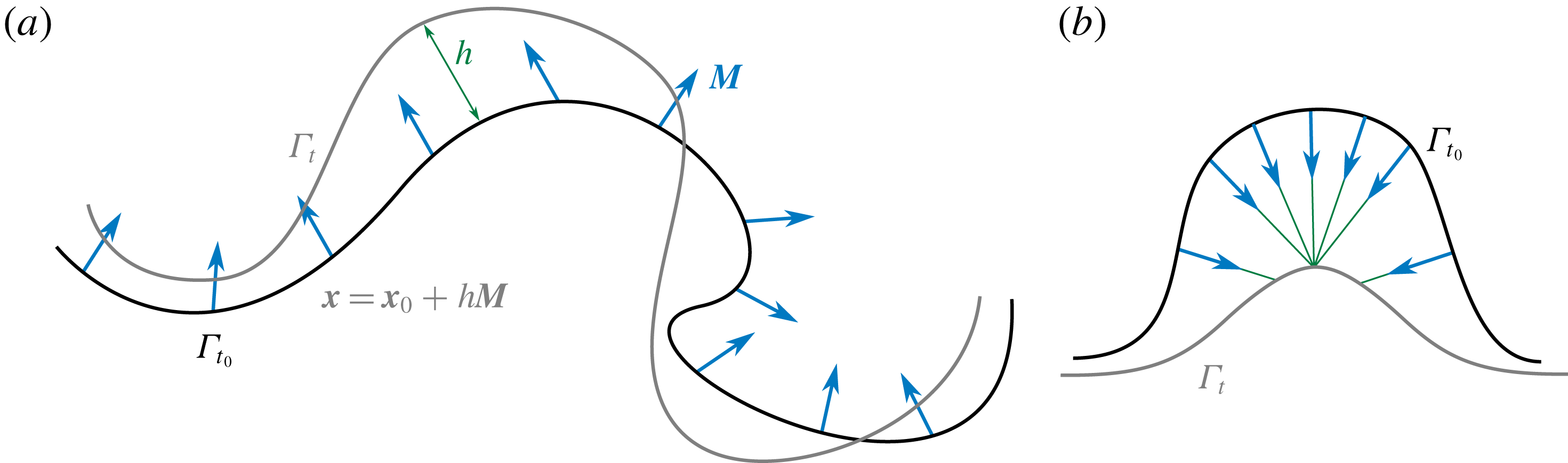
Surface parametrization in terms of an offset. (a) The field of directors
 $\boldsymbol{M}$
represents the direction in which the point
 $\boldsymbol{x}_{0}\in \unicode[STIX]{x1D6E4}_{t_{0}}$
can evolve. The height function
 $h$
, which may be negative, represents the distance between the point
 $\boldsymbol{x}$
on
 $\unicode[STIX]{x1D6E4}_{t}$
and
 $\unicode[STIX]{x1D6E4}_{t_{0}}$
in the direction of
 $\boldsymbol{M}$
. (b) In this example
 $\unicode[STIX]{x1D6E4}_{t}$
lies at the limit of the tubular neighbourhood to
 $\unicode[STIX]{x1D6E4}_{t_{0}}$
for the given director field.

We define next a restricted ALE parametrization, which by construction is devoid of the arbitrary freedom associated with tangential motions. Let us consider the state of the surface at a given time
 $t_{0}$
,
 $\unicode[STIX]{x1D6E4}_{t_{0}}$
, and a parametrization of this surface
 $\unicode[STIX]{x1D74D}_{0}(\unicode[STIX]{x1D743})$
. We consider a vector field
 $\boldsymbol{M}(\unicode[STIX]{x1D743})$
, representing a field of directors over
 $\unicode[STIX]{x1D6E4}_{t_{0}}$
, with non-zero normal component but not necessarily coinciding with the normal field of
 $\unicode[STIX]{x1D6E4}_{t_{0}}$
. We define a family of parametrizations of
 $\unicode[STIX]{x1D6E4}_{t}$
at time
 $t>t_{0}$
in terms of the offset of a point
 $\boldsymbol{x}=\unicode[STIX]{x1D74D}_{0}(\unicode[STIX]{x1D743})$
along
 $\boldsymbol{M}(\unicode[STIX]{x1D743})$
,
 $$\begin{eqnarray}\unicode[STIX]{x1D74D}(\unicode[STIX]{x1D743},t)=\unicode[STIX]{x1D74D}_{0}(\unicode[STIX]{x1D743})+h(\unicode[STIX]{x1D743},t)\boldsymbol{M}(\unicode[STIX]{x1D743}),\end{eqnarray}$$
see figure 3(a). The field that characterizes the time evolution of the parametrization is
 $h$
, a simple scalar field on
 $\tilde{\unicode[STIX]{x1D6E4}}$
. This approach is not completely general, since it only allows us to parametrize the surfaces lying in the so-called tubular neighbourhood of
 $\unicode[STIX]{x1D6E4}_{t_{0}}$
(do Carmo Reference do Carmo2016). However, for some interval
 $I=(t_{0},t_{0}+\unicode[STIX]{x1D6FF}t)$
, the deformed surface
 $\unicode[STIX]{x1D6E4}_{t}$
will lie in the tubular neighbourhood of
 $\unicode[STIX]{x1D6E4}_{t_{0}}$
if the time evolution is smooth. To deal with the fact that after some time
 $\unicode[STIX]{x1D6E4}_{t}$
may leave the tubular neighbourhood of
 $\unicode[STIX]{x1D6E4}_{t_{0}}$
(see figure 3
b), a simple solution is to periodically update the reference configuration
 $\unicode[STIX]{x1D6E4}_{t_{0}}$
. This kind of parametrization, proposed by Rangarajan & Gao (Reference Rangarajan and Gao2015), generalizes the classical Monge parametrization, which is recovered by setting
 $\unicode[STIX]{x1D6E4}_{t_{0}}$
to a plane,
 $\boldsymbol{M}$
to its constant normal and
 $h$
to the height of the surface
 $\unicode[STIX]{x1D6E4}_{t}$
with respect to the plane (do Carmo Reference do Carmo2016). We finally note that for this kind of surface parametrization, we have
 $$\begin{eqnarray}\boldsymbol{W}(\boldsymbol{x},t)=(\unicode[STIX]{x2202}_{t}h\,\boldsymbol{M})\circ \unicode[STIX]{x1D74D}^{-1}(\boldsymbol{x},t).\end{eqnarray}$$
Since
 $h$
is a scalar field on
 $\tilde{\unicode[STIX]{x1D6E4}}$
,
 $\unicode[STIX]{x2202}_{t}h$
in this equation has the usual meaning of time differentiation at fixed
 $\unicode[STIX]{x1D743}$
. In practice,
 $\boldsymbol{M}$
can be chosen to be
 $\boldsymbol{N}_{0}$
, the field of normals of the reference surface as in (Rangarajan & Gao Reference Rangarajan and Gao2015). This leads to an Eulerian parametrization at
 $t=t_{0}$
, and close to it at later times. Thus,
 $\boldsymbol{W}$
will have in general non-zero tangential components, and therefore this parametrization is neither Eulerian nor Lagrangian. Instead, it is an ALE parametrization depending on a generalized height field
 $h$
, in which the arbitrariness is removed by following (2.31) and choosing the field of directors
 $\boldsymbol{M}$
.
2.5.2 Velocity potentials: Hodge decomposition
Given a vector field
 $\boldsymbol{V}\in \mathbb{R}^{3}$
, it is well known that
 $\boldsymbol{V}$
admits a decomposition in terms of the gradient of a function
 $\unicode[STIX]{x1D6F7}$
and the curl of a vector potential
 $\boldsymbol{A}$
in what is called the Helmholtz decomposition,
 $$\begin{eqnarray}\boldsymbol{V}=\unicode[STIX]{x1D735}\,\unicode[STIX]{x1D6F7}+\unicode[STIX]{x1D735}\times \,\boldsymbol{A},\end{eqnarray}$$
where here
 $\unicode[STIX]{x1D735}$
and
 $\unicode[STIX]{x1D735}\times$
stand for the gradient and curl in
 $\mathbb{R}^{3}$
. For a vector field tangent to a plane embedded in
 $\mathbb{R}^{3}$
, this can be simplified to
 $$\begin{eqnarray}\boldsymbol{V}=\unicode[STIX]{x1D735}\,\unicode[STIX]{x1D6F7}+\unicode[STIX]{x1D735}\times (\unicode[STIX]{x1D6F9}\boldsymbol{N}),\end{eqnarray}$$
where
 $\boldsymbol{N}$
is the normal to the plane and
 $\unicode[STIX]{x1D6F9}$
is a scalar function. Therefore, for a plane embedded in
 $\mathbb{R}^{3}$
, a tangent vector field can be represented in terms of two scalar fields,
 $\unicode[STIX]{x1D6F7}$
and
 $\unicode[STIX]{x1D6F9}$
. This property can be generalized to arbitrary surfaces in terms of their intrinsic differential geometry, i.e. not relying on their embedding in
 $\mathbb{R}^{3}$
, as a special case of the Hodge decomposition for
 $n$
-forms (do Carmo Reference do Carmo1992). A vector field
 $\boldsymbol{v}$
tangent to a surface
 $\unicode[STIX]{x1D6E4}$
can be decomposed as
 $$\begin{eqnarray}\boldsymbol{v}=\unicode[STIX]{x1D735}\unicode[STIX]{x1D6FC}+\unicode[STIX]{x1D735}\times \unicode[STIX]{x1D6FD}+\boldsymbol{h},\end{eqnarray}$$
where
 $\unicode[STIX]{x1D6FC}$
and
 $\unicode[STIX]{x1D6FD}$
are scalar fields on
 $\unicode[STIX]{x1D6E4}$
and
 $\boldsymbol{h}$
is a harmonic vector field, satisfying
 $\unicode[STIX]{x1D735}\boldsymbol{\cdot }\boldsymbol{h}=0$
and
 $\unicode[STIX]{x1D735}\times \boldsymbol{h}=0$
. We note that the curl operator
 $\unicode[STIX]{x1D735}\times$
on a surface, an instance of exterior derivative, is defined differently to its counterpart in Euclidean space. For instance, applied on a scalar function
 $\unicode[STIX]{x1D735}\times \unicode[STIX]{x1D6FD}$
is a vector with components
 $(\unicode[STIX]{x1D735}\times \unicode[STIX]{x1D6FD})^{a}=\unicode[STIX]{x1D716}^{ab}\unicode[STIX]{x1D735}_{b}\unicode[STIX]{x1D6FD}$
, where
 $\unicode[STIX]{x1D750}$
is the antisymmetric tensor
 $$\begin{eqnarray}\unicode[STIX]{x1D750}^{ab}=J^{-1}\unicode[STIX]{x1D700}^{ab},\end{eqnarray}$$
with
 $\unicode[STIX]{x1D700}^{ab}$
the Levi-Civita symbols, defined by
 $\unicode[STIX]{x1D700}^{11}=\unicode[STIX]{x1D700}^{22}=0$
,
 $\unicode[STIX]{x1D700}^{12}=-\unicode[STIX]{x1D700}^{21}=1$
. For simply connected surfaces, i.e. closed surfaces with genus equal to 0, there is only a trivial harmonic vector field,
 $\boldsymbol{h}=\mathbf{0}$
, and
 $\boldsymbol{v}$
can be described in terms of the two scalar fields
 $\unicode[STIX]{x1D6FC}$
and
 $\unicode[STIX]{x1D6FD}$
(see figure 4 for an example on an ellipsoid). In the absence of shape changes, from (2.30) it is clear that an inextensible flow satisfies
 $\unicode[STIX]{x1D735}\boldsymbol{\cdot }\boldsymbol{v}=0$
. In this case,
 $\boldsymbol{v}$
can be represented in terms of a streamfunction as
 $\boldsymbol{v}=\unicode[STIX]{x1D735}\times \unicode[STIX]{x1D6FD}$
. This approach was introduced by Secomb & Skalak (Reference Secomb and Skalak1982) to describe flows in fluid surfaces with fixed shape and used more recently by various authors (Nitschke et al.
Reference Nitschke, Voigt and Wensch2012; Morris & Turner Reference Morris and Turner2015; Reuther & Voigt Reference Reuther and Voigt2015, Reference Reuther and Voigt2016; Sigurdsson & Atzberger Reference Sigurdsson and Atzberger2016; Gross & Atzberger Reference Gross and Atzberger2018; Mickelin et al.
Reference Mickelin, Słomka, Burns, Lecoanet, Vasil, Faria and Dunkel2018). However, we note that for inextensible surfaces that change shape, both
 $\unicode[STIX]{x1D6FC}$
and
 $\unicode[STIX]{x1D6FD}$
need be considered. In this case, using the fact that
 $\unicode[STIX]{x1D735}\boldsymbol{\cdot }\boldsymbol{v}=\unicode[STIX]{x1D735}\boldsymbol{\cdot }\unicode[STIX]{x1D735}\unicode[STIX]{x1D6FC}+\unicode[STIX]{x1D735}\boldsymbol{\cdot }\unicode[STIX]{x1D735}\times \unicode[STIX]{x1D6FD}=\unicode[STIX]{x1D735}\boldsymbol{\cdot }\unicode[STIX]{x1D735}\unicode[STIX]{x1D6FC}=\unicode[STIX]{x0394}\unicode[STIX]{x1D6FC}$
, where
 $\unicode[STIX]{x0394}\unicode[STIX]{x1D6FC}=\unicode[STIX]{x1D735}\boldsymbol{\cdot }\unicode[STIX]{x1D735}\unicode[STIX]{x1D6FC}$
, it follows from (2.30) that in an inextensible flow
 $\unicode[STIX]{x1D6FC}$
and
 $v_{n}$
satisfy the constraint
 $$\begin{eqnarray}\unicode[STIX]{x0394}\unicode[STIX]{x1D6FC}=v_{n}H.\end{eqnarray}$$
This approach has been recently considered to examine flows on a time-evolving inextensible membrane with prescribed shape changes (Reuther & Voigt Reference Reuther and Voigt2018a ).
A vector field on a simply connected surface can be decomposed as the sum of a solenoidal and an irrotational field.

3 Physical models of fluid surfaces
In this section we examine classical models for fluid deformable surfaces, two used to model lipid bilayers and one applicable to the cell cortex. Thanks to the tools introduced above and Onsager’s formalism, we derive the corresponding governing equations in their full three-dimensional and nonlinear generality.
3.1 Lipid bilayers: an inextensible viscous layer with bending energy
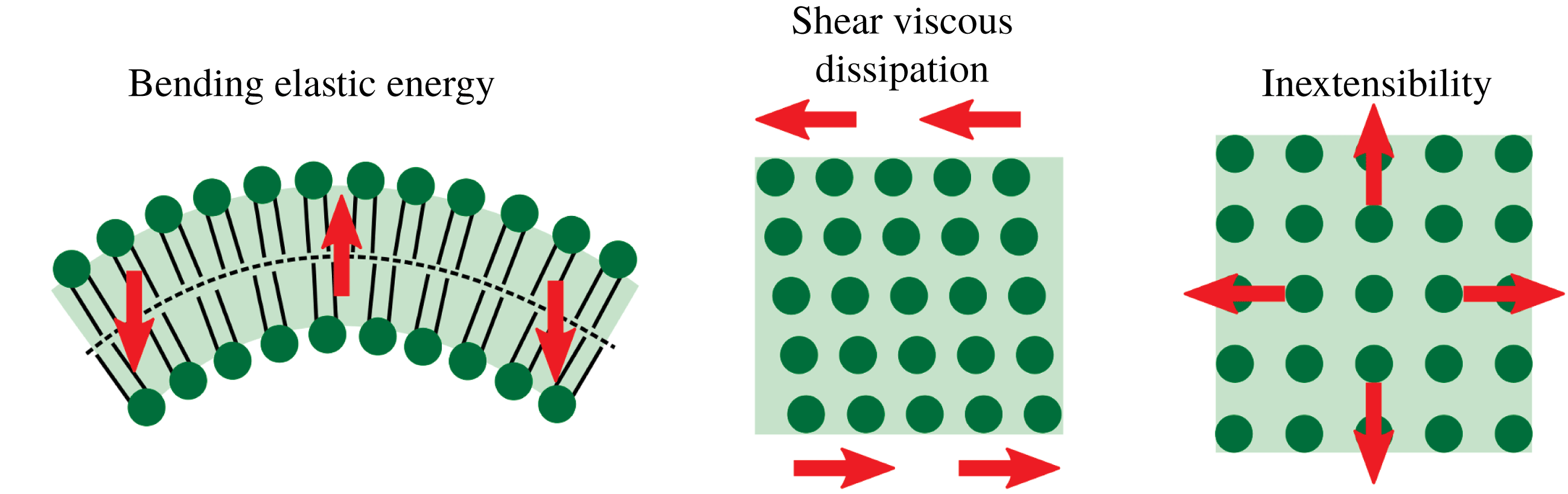
Lipid membranes are interfacial viscous fluids with bending elasticity. The interplay between viscosity and elasticity determines their relaxation dynamics after they are brought out of equilibrium by external forces or biological activity. These two essential mechanical features of lipid membranes, their out-of-plane elasticity and interfacial viscosity, have often been examined separately. The mechanical equilibrium of lipid bilayers can be understood to a large extent with the classical bending model of Helfrich (Helfrich Reference Helfrich1973; Lipowsky Reference Lipowsky1991; Jülicher & Lipowsky Reference Jülicher and Lipowsky1993). For that reason, studies of lipid bilayers at scales beyond tens of nanometres have mainly focused on this model, e.g. in investigations of equilibrium configurations of closed vesicles under geometric constraints, such as fixed surface area or fixed enclosed volume (Steigmann Reference Steigmann1999; Capovilla & Guven Reference Capovilla and Guven2002; Tu & Ou-Yang Reference Tu and Ou-Yang2004; Feng & Klug Reference Feng and Klug2006; Rangarajan & Gao Reference Rangarajan and Gao2015; Sauer et al. Reference Sauer, Duong, Mandadapu and Steigmann2017). Beyond the Helfrich model, and subsequent refinements such as the area difference elasticity model (Miao et al. Reference Miao, Seifert, Wortis and Döbereiner1994; Seifert Reference Seifert1997), more general models are required to describe the dynamical transformations that bilayers undergo, which should capture the interfacial dissipative mechanisms that dominate at sub-cellular scales. In a discrete stochastic approach based on dynamically triangulated surfaces (Ho & Baumgärtner Reference Ho and Baumgärtner1990), shape transformations of fluid vesicles (Kroll & Gompper Reference Kroll and Gompper1992; Gompper & Kroll Reference Gompper and Kroll2004) or their dynamics under flow (Noguchi & Gompper Reference Noguchi and Gompper2005; Peng et al. Reference Peng, Li, Pivkin, Dao, Karniadakis and Suresh2013) have been examined. From a continuum viewpoint, the interfacial hydrodynamics of bilayer membranes was first examined separately from membrane deformation, i.e. assuming fixed membrane shape. These studies focused on the mobility of membrane inclusions, such as proteins, starting with the seminal work of Saffman & Delbrück (Reference Saffman and Delbrück1975) on planar lipid bilayers. Subsequent studies have considered the effect of fluid boundaries (Stone & Ajdari Reference Stone and Ajdari1998) or the (fixed) shape of the fluid membrane (Levine, Liverpool & MacKintosh Reference Levine, Liverpool and MacKintosh2004; Henle & Levine Reference Henle and Levine2010; Sigurdsson & Atzberger Reference Sigurdsson and Atzberger2016). Interfacial flows of vesicles induced by shear bulk flows were also considered at fixed vesicle shape (Secomb & Skalak Reference Secomb and Skalak1982). Following the seminal works of Scriven (Reference Scriven1960) and Aris (Reference Aris1962) on the hydrodynamics of insoluble fluid films, Barthes-Biesel & Sgaier (Reference Barthes-Biesel and Sgaier1985) examined the interfacial flow of vesicles in a shear flow allowing for infinitesimal shape deformations. More recently, a geometrically nonlinear model for an inextensible viscous interfacial fluid with bending rigidity was examined, formulated geometrically, and exercised under the assumption of axisymmetry (Arroyo & DeSimone Reference Arroyo and DeSimone2009; Arroyo et al. Reference Arroyo, DeSimone and Heltai2010). Along these lines, there is an increasing interest in the community of applied and computational mathematics to develop numerical methods to solve the three-dimensional equations governing inextensible viscous interfaces with curvature elasticity (Nitschke et al. Reference Nitschke, Voigt and Wensch2012; Rodrigues et al. Reference Rodrigues, Ausas, Mut and Buscaglia2015; Barrett et al. Reference Barrett, Garcke and Nürnberg2016; Reuther & Voigt Reference Reuther and Voigt2016). This model provides a first approximation to the dynamical behaviour of lipid membranes, see figure 5.
A simple model of a lipid bilayer as an inextensible viscous fluid with bending elasticity.

Here, we formulate this model based on Onsager’s variational formalism (Arroyo & DeSimone Reference Arroyo and DeSimone2009), and derive the Euler–Lagrange equations. Considering a membrane without spontaneous curvature and ignoring the Gaussian curvature term in the Helfrich Hamiltonian, the bending energy of the membrane can be written as
 $$\begin{eqnarray}{\mathcal{F}}_{H}[\unicode[STIX]{x1D753}]=\int _{\unicode[STIX]{x1D6E4}_{t}}\frac{\unicode[STIX]{x1D705}}{2}H^{2}\,\text{d}S,\end{eqnarray}$$
where
 $\unicode[STIX]{x1D705}$
is the bending modulus. The free energy depends on the set of state variables of the system, usually denoted by
 $X$
. In this case, the material parametrization is the state variable of the system,
 $X=\{\unicode[STIX]{x1D753}\}$
. We note, however, that since the energy only depends on the shape of
 $\unicode[STIX]{x1D6E4}_{t}$
,
 $\unicode[STIX]{x1D753}$
can be replaced by any other ALE parametrization
 $\unicode[STIX]{x1D74D}$
. In Onsager’s variational formalism, dissipative mechanisms are introduced through dissipation potentials. The Newtonian shear rheology of lipid membranes (Dimova et al.
Reference Dimova, Aranda, Bezlyepkina, Nikolov, Riske and Lipowsky2006) is encoded in the following dissipation potential
 $$\begin{eqnarray}{\mathcal{D}}_{S}[\unicode[STIX]{x1D753};\boldsymbol{V}]=\int _{\unicode[STIX]{x1D6E4}_{t}}\unicode[STIX]{x1D707}|\unicode[STIX]{x1D659}|^{2}\,\text{d}S,\end{eqnarray}$$
where
 $\unicode[STIX]{x1D707}$
is the (in-plane) shear viscosity of the monolayer and
 $|\unicode[STIX]{x1D659}|^{2}=d_{ab}\unicode[STIX]{x1D628}^{ac}\unicode[STIX]{x1D628}^{bd}d_{cd}$
. Since we assume that the deformation of the membrane is inextensible, only the deviatoric part of
 $\unicode[STIX]{x1D659}$
matters in the above definition. The dissipation potential depends on the state variable of the system,
 $\unicode[STIX]{x1D753}$
, through shape in
 $\text{d}S$
and
 $\unicode[STIX]{x1D65C}$
, but primarily on the variable representing the rate of change of the state,
 $\boldsymbol{V}$
. The variables that represent the processes that change the state of the system and produce dissipation are called process variables and denoted by
 $V$
; here
 $V=\{\boldsymbol{V}\}$
. Here the process variable is simply the time derivative of the state variable
 $\boldsymbol{V}=\unicode[STIX]{x2202}_{t}\unicode[STIX]{x1D753}$
, but this is not necessarily the case. For instance, if we had used
 $\unicode[STIX]{x1D74D}$
rather than
 $\unicode[STIX]{x1D753}$
as state variable, then
 $\boldsymbol{W}=\unicode[STIX]{x2202}_{t}\unicode[STIX]{x1D74D}$
would not be a meaningful variable to encode dissipation since it does not represent a physical velocity. For thermodynamical consistency, the dissipation potential
 ${\mathcal{D}}(X;V)$
must be a convex function of
 $V$
with minimum at
 $V=0$
(Arroyo et al.
Reference Arroyo, Walani, Torres-Sánchez, Kaurin and Steigmann2018). We further assume that
 ${\mathcal{D}}(X;0)=0$
, so that
 ${\mathcal{D}}(X;V)\geqslant 0$
. If external forces
 $\boldsymbol{F}$
are applied, these introduce a power input
 $$\begin{eqnarray}{\mathcal{P}}[\unicode[STIX]{x1D753};\boldsymbol{V}]=-\int _{\unicode[STIX]{x1D6E4}_{t}}\boldsymbol{F}\boldsymbol{\cdot }\boldsymbol{V}\,\text{d}S.\end{eqnarray}$$
One can also include the dissipation potential associated with the bulk viscous fluid where the membrane is embedded. Here, we ignore bulk hydrodynamical forces to focus on the fluid membrane, an assumption which is physically justified for phenomena below the Saffman–Delbrück length scale
 $l_{SD}=\unicode[STIX]{x1D707}/\unicode[STIX]{x1D707}_{b}$
, where
 $\unicode[STIX]{x1D707}_{b}$
is the bulk viscosity (Saffman & Delbrück Reference Saffman and Delbrück1975; Arroyo & DeSimone Reference Arroyo and DeSimone2009). For a lipid membrane,
 $l_{SD}\approx 5~\unicode[STIX]{x03BC}\text{m}$
.
Onsager’s variational principle establishes a competition between energy release rate, power and dissipation through the Rayleighian, which takes the form
 $$\begin{eqnarray}{\mathcal{R}}[\unicode[STIX]{x1D753};\boldsymbol{V}]=D_{t}{\mathcal{F}}_{H}[\unicode[STIX]{x1D753};\boldsymbol{V}]+{\mathcal{D}}_{S}[\unicode[STIX]{x1D753};\boldsymbol{V}]+{\mathcal{P}}[\unicode[STIX]{x1D753};\boldsymbol{V}].\end{eqnarray}$$
Here, the rate of change of the energy
 $D_{t}{\mathcal{F}}_{H}[\unicode[STIX]{x1D753};\boldsymbol{V}]$
is
 $$\begin{eqnarray}D_{t}{\mathcal{F}}_{H}[\unicode[STIX]{x1D753};\boldsymbol{V}]=\int _{\unicode[STIX]{x1D6E4}_{t}}\unicode[STIX]{x1D705}\left\{H\unicode[STIX]{x0394}v_{n}-\left(\frac{1}{2}H^{2}-|\boldsymbol{k}|^{2}\right)Hv_{n}+\unicode[STIX]{x1D735}_{a}\left(\frac{1}{2}\unicode[STIX]{x1D705}H^{2}v^{a}\right)\right\}\,\text{d}S,\end{eqnarray}$$
where we have used that
 $\unicode[STIX]{x2202}_{t}H=\unicode[STIX]{x0394}v_{n}+|\boldsymbol{k}|^{2}v_{n}$
(Capovilla & Guven Reference Capovilla and Guven2002; Arroyo & DeSimone Reference Arroyo and DeSimone2009). Then, Onsager’s principle states that process variables minimize the Rayleighian
 $$\begin{eqnarray}\boldsymbol{V}=\underset{\boldsymbol{U}}{\arg \min }\,{\mathcal{R}}[\unicode[STIX]{x1D753};\boldsymbol{U}],\end{eqnarray}$$
subject to constraints
 $Q[\unicode[STIX]{x1D753};\boldsymbol{V}]$
. Here, we consider that the surface is inextensible
 $$\begin{eqnarray}Q_{1}[\unicode[STIX]{x1D753};\boldsymbol{V}]=\text{tr}\,\unicode[STIX]{x1D659}=\unicode[STIX]{x1D735}\boldsymbol{\cdot }\boldsymbol{v}-v_{n}H=0.\end{eqnarray}$$
Furthermore, due to osmotic effects, it can often be assumed that cells and vesicles maintain constant volume, and hence
 $$\begin{eqnarray}Q_{2}[\unicode[STIX]{x1D753};\boldsymbol{V}]=\int _{\unicode[STIX]{x1D6E4}_{t}}\boldsymbol{V}\boldsymbol{\cdot }\boldsymbol{N}\,\text{d}S=0.\end{eqnarray}$$
To enforce these constraints, we can introduce the Lagrangian
 $$\begin{eqnarray}{\mathcal{L}}[\unicode[STIX]{x1D753};\boldsymbol{V},\unicode[STIX]{x1D6FE},P]={\mathcal{R}}[\unicode[STIX]{x1D753};\boldsymbol{V}]+\int _{\unicode[STIX]{x1D6E4}_{t}}\unicode[STIX]{x1D6FE}Q_{1}[\unicode[STIX]{x1D753};\boldsymbol{V}]\,\text{d}S-PQ_{2}[\unicode[STIX]{x1D753};\boldsymbol{V}].\end{eqnarray}$$
 $P$
is the pressure in the vesicle and
 $\unicode[STIX]{x1D6FE}$
is a component of the surface tension. Then, Onsager’s principle subject to constraints can be written as a saddle-point problem
 $$\begin{eqnarray}\{\boldsymbol{V},\unicode[STIX]{x1D6FE},P\}=\underset{\boldsymbol{U}}{\arg \min }~\underset{\unicode[STIX]{x1D706},S}{\arg \max }{\mathcal{L}}[\unicode[STIX]{x1D753};\boldsymbol{U},\unicode[STIX]{x1D706},S].\end{eqnarray}$$
From the stationarity conditions of (3.10), one finds the weak and the strong form of the governing equations (see appendix D), the latter of which take the form
 $$\begin{eqnarray}\displaystyle & \displaystyle \unicode[STIX]{x1D735}_{a}\unicode[STIX]{x1D72E}^{a}+\boldsymbol{B}=\mathbf{0}, & \displaystyle\end{eqnarray}$$
 $$\begin{eqnarray}\displaystyle & \displaystyle \text{tr}\,\unicode[STIX]{x1D659}=0, & \displaystyle\end{eqnarray}$$
 $$\begin{eqnarray}\displaystyle & \displaystyle \int _{\unicode[STIX]{x1D6E4}_{t}}\boldsymbol{V}\boldsymbol{\cdot }\boldsymbol{N}\,\text{d}S=0. & \displaystyle\end{eqnarray}$$
Here,
 $\unicode[STIX]{x1D72E}^{a}$
is the so-called surface stress vector,
 $$\begin{eqnarray}\unicode[STIX]{x1D72E}^{a}=\unicode[STIX]{x1D70E}^{ab}\boldsymbol{e}_{b}+\unicode[STIX]{x1D70E}_{n}^{a}\boldsymbol{N},\end{eqnarray}$$
where
 $\unicode[STIX]{x1D748}$
is the in-plane stress
 $$\begin{eqnarray}\unicode[STIX]{x1D70E}^{ab}=\unicode[STIX]{x1D705}H({\textstyle \frac{1}{2}}H\unicode[STIX]{x1D628}^{ab}-k^{ab})+2\unicode[STIX]{x1D707}\unicode[STIX]{x1D625}^{ab}+\unicode[STIX]{x1D6FE}\unicode[STIX]{x1D628}^{ab},\end{eqnarray}$$
and
 $\unicode[STIX]{x1D748}_{n}$
is a vector of normal stresses
 $$\begin{eqnarray}\unicode[STIX]{x1D70E}_{n}^{a}=-\unicode[STIX]{x1D705}\unicode[STIX]{x1D628}^{ab}\unicode[STIX]{x1D735}_{b}H.\end{eqnarray}$$
When multiplied by a unit vector
 $\boldsymbol{l}$
in
 $T_{\boldsymbol{x}}\unicode[STIX]{x1D6E4}_{t}$
,
 $\unicode[STIX]{x1D72E}^{b}l_{b}$
is the three-dimensional force per unit length across a curve passing through
 $\boldsymbol{x}$
and perpendicular to
 $\boldsymbol{l}$
. Note that
 $\unicode[STIX]{x1D70E}_{n}^{a}$
represents bending moments caused by curvature imbalances. Finally,
 $\boldsymbol{B}$
is the field of (external) body forces
 $$\begin{eqnarray}\boldsymbol{B}=\boldsymbol{F}+P\boldsymbol{N}.\end{eqnarray}$$
Equations (3.11)–(3.13) express the balance of linear momentum and conservation of mass (inextensibility) and enclosed volume in a fully nonlinear regime. Alternatively, one could have derived equation (3.11) from a local force balance on the membrane as in Salbreux & Jülicher (Reference Salbreux and Jülicher2017), and postulated the constitutive laws (3.15) and (3.16). Thus, by starting from different ingredients (a Rayleighian expressing energy release-rate, dissipation and power input) and invoking a variational principle subject to constraints, Onsager’s formalism recovers these equations in a systematic and transparent way. As a direct corollary of Onsager’s principle, it is easy to see that, in the absence of external power inputs, the free energy is a Lyapunov functional of the dynamics, i.e.
 ${\mathcal{F}}$
is a decreasing functional (Arroyo et al.
Reference Arroyo, Walani, Torres-Sánchez, Kaurin and Steigmann2018)
 $$\begin{eqnarray}D_{t}{\mathcal{F}}\leqslant 0,\end{eqnarray}$$
which provides a nonlinear notion of stability for the dynamics. From a computational point of view, only the weak form of the stationarity conditions issuing from Onsager’s formalism is required for a space discretization based on finite elements. Onsager’s formalism also provides a framework to formulate nonlinearly stable variational time integrators, as described in § 4.
We finally note that the choice of state and process variables is not unique. For instance, as mentioned earlier, we can choose an ALE parametrization
 $\unicode[STIX]{x1D74D}$
instead of
 $\unicode[STIX]{x1D753}$
as state variable, since the free energy depends only on shape. The velocity
 $\boldsymbol{V}$
, our process variable, then needs to be split into a normal and a tangential components
 $\boldsymbol{V}=\boldsymbol{v}+v_{n}\boldsymbol{N}$
, where
 $v_{n}=\boldsymbol{W}\boldsymbol{\cdot }\boldsymbol{N}$
. For the ALE parametrization in (2.31), we have
 $v_{n}=\unicode[STIX]{x2202}_{t}h\boldsymbol{M}\boldsymbol{\cdot }\boldsymbol{N}$
. We can then rewrite the Lagrangian in terms of
 $\unicode[STIX]{x2202}_{t}h$
and
 $\boldsymbol{v}$
. We can further decompose
 $\boldsymbol{v}=\unicode[STIX]{x1D735}\unicode[STIX]{x1D6FC}+\unicode[STIX]{x1D735}\times \unicode[STIX]{x1D6FD}$
. Then, the governing equations for this set of variables follow from
 $$\begin{eqnarray}\underset{\unicode[STIX]{x2202}_{t}h,\unicode[STIX]{x1D6FC},\unicode[STIX]{x1D6FD}}{\min }~\underset{\unicode[STIX]{x1D6FE},P}{\max }\,{\mathcal{L}}[h;\unicode[STIX]{x2202}_{t}h,\unicode[STIX]{x1D6FC},\unicode[STIX]{x1D6FD},\unicode[STIX]{x1D6FE},P].\end{eqnarray}$$
The Euler–Lagrange equations resulting from this statement will look very different from those in (3.10) but describe the same dynamics. While the choice of variables
 $X=\{\unicode[STIX]{x1D753}\}$
and
 $V=\{\boldsymbol{V}\}$
is natural from a modelling viewpoint, the choice
 $X=\{h\}$
and
 $V=\{v_{n},\unicode[STIX]{x1D6FC},\unicode[STIX]{x1D6FD}\}$
is better suited from a computational viewpoint, as will become clear in § 4. In appendix G we provide detailed expressions for the algebraic optimization problem that we solve numerically and that results from discretizing equation (3.19) in space and time.
3.2 Lipid bilayers: the Seifert–Langer model
The previous model provides a first approach to the mechanics of lipid bilayers. It is often overlooked, however, that by ignoring the bilayer architecture it fails to capture many important phenomena. Seifert and Langer developed a continuum model explicitly accounting for the bilayer architecture and capturing the major energetic driving forces and dissipative drag forces involved in the dynamics of lipid membranes (Seifert & Langer Reference Seifert and Langer1993). The elastic forces in this theory appear in response to bending of the membrane, as in the previous model, but also to monolayer stretching (see figure 6). As viscous effects, the in-plane Newtonian rheology of the lipid bilayer (Dimova et al. Reference Dimova, Aranda, Bezlyepkina, Nikolov, Riske and Lipowsky2006) is included through shear and dilatation dissipations, and the frictional coupling between the two monolayers opposing inter-monolayer slippage is also included. This model provided predictions about the relaxation dynamics of membrane fluctuations. Importantly, its material parameters can be experimentally measured (Dimova et al. Reference Dimova, Aranda, Bezlyepkina, Nikolov, Riske and Lipowsky2006). The work of Seifert & Langer (Reference Seifert and Langer1993), along with Evans & Yeung (Reference Evans and Yeung1994), highlighted the role of inter-monolayer friction as a ‘hidden’ but significant dissipative effect. This physical model was originally introduced and has been predominantly exercised under the restricted assumptions of linearized disturbances around a planar (Seifert & Langer Reference Seifert and Langer1993; Fournier Reference Fournier2015) or cylindrical state (Nelson, Powers & Seifert Reference Nelson, Powers and Seifert1995) or of simplified and fixed membrane shape (Evans & Yeung Reference Evans and Yeung1994). These approximations, however, hide much of the interaction between shape dynamics and interfacial hydrodynamics, which is mediated by membrane curvature. This was demonstrated by the linearization of the theory about spherical or cylindrical configurations (Rahimi Reference Rahimi2013) and by simulations based on a fully nonlinear version of this theory, albeit axisymmetric (Rahimi & Arroyo Reference Rahimi and Arroyo2012), which further demonstrated the geometry-dependent subtle interplay between all the ingredients in figure 6 at multiple scales. Seifert and Langer’s (SL) model is conceptually simple, captures sufficient physics to describe a plethora of dynamical phenomena, and can be the basis for more sophisticated dynamical models including for instance lipid tilt near molecular inclusions (Hamm & Kozlov Reference Hamm and Kozlov1998, Reference Hamm and Kozlov2000) or the physicochemical interaction of lipids with scaffolding or integral proteins (Brochard-Wyart & de Gennes Reference Brochard-Wyart and de Gennes2002; Arroyo et al. Reference Arroyo, Walani, Torres-Sánchez, Kaurin and Steigmann2018). Here we formulate and develop numerical calculations with this model in a three-dimensional and fully nonlinear set-up which, to our best knowledge, has not been examined before.
In a basic model incorporating elasticity and hydrodynamics (Seifert & Langer Reference Seifert and Langer1993), a lipid bilayer stores energy due to bending and monolayer stretching and dissipates energy through shear, dilatation and inter-monolayer friction. To describe this model mathematically, the densities at the monolayer mid-surfaces
 $\breve{\unicode[STIX]{x1D70C}}^{\pm }$
are projected onto the bilayer mid-surface leading to the scalar fields
 $\unicode[STIX]{x1D70C}^{\pm }:\unicode[STIX]{x1D6E4}_{t}\rightarrow \mathbb{R}$
. The velocity fields
 $\boldsymbol{v}^{\pm }$
identify the velocity of the material particles at
 $\unicode[STIX]{x1D6E4}_{t}$
.

In this model,
 $\unicode[STIX]{x1D6E4}_{t}$
characterizes the bilayer mid-surface (see figure 6). In addition to the Helfrich energy of the form of (3.1), the Seifert–Langer model accounts for the stretching elasticity of each of the monolayers through the functional
 $$\begin{eqnarray}{\mathcal{F}}_{S}[\unicode[STIX]{x1D74C},\unicode[STIX]{x1D70C}^{\pm }]=\int _{\unicode[STIX]{x1D6E4}_{t}}\frac{k_{S}}{2}(\breve{\unicode[STIX]{x1D70C}}^{\pm }-1)^{2}\,\text{d}S=\int _{\unicode[STIX]{x1D6E4}_{t}}\frac{k_{S}}{2}[\unicode[STIX]{x1D70C}^{\pm }(1\pm \,\text{d}H)-1]^{2}\,\text{d}S,\end{eqnarray}$$
where the fields
 $\breve{\unicode[STIX]{x1D70C}}^{\pm }$
represent the lipid density at the neutral surface of the upper
 $(+)$
and lower
 $(-)$
monolayers, measured in units of the equilibrium density, which differ from the lipid density at the bilayer mid-surface according to
 $$\begin{eqnarray}\breve{\unicode[STIX]{x1D70C}}=\unicode[STIX]{x1D70C}^{\pm }(1\pm \,\text{d}H)+O(Kd^{2}),\end{eqnarray}$$
with
 $d\approx 1~\text{nm}$
the distance between the neutral surfaces and the bilayer mid-surface. Unless otherwise noted, a functional containing
 $\pm$
implies a summation on the
 $+$
and
 $-$
monolayers. For convenience, in this section we use an Eulerian parametrization
 $\unicode[STIX]{x1D74C}$
to derive the governing equations. The free energy depends on
 $\unicode[STIX]{x1D74C}$
and the two density fields
 $\unicode[STIX]{x1D70C}^{+}$
and
 $\unicode[STIX]{x1D70C}^{-}$
, representing the density of lipids on the mid-surface, and thus
 $X=\{\unicode[STIX]{x1D74C},\unicode[STIX]{x1D70C}^{+},\unicode[STIX]{x1D70C}^{-}\}$
. We take into account three main dissipation mechanisms in the bilayer. First we consider the dissipation due to in-plane shear in each monolayer, which takes the form
 $$\begin{eqnarray}{\mathcal{D}}_{S}[\unicode[STIX]{x1D74C};v_{n},\boldsymbol{v}^{\pm }]=\int _{\unicode[STIX]{x1D6E4}_{t}}\unicode[STIX]{x1D707}|\unicode[STIX]{x1D659}^{\pm }|^{2}\,\text{d}S,\end{eqnarray}$$
where
 $\unicode[STIX]{x1D707}$
is the shear viscosity and
 $$\begin{eqnarray}\unicode[STIX]{x1D659}^{\pm }={\textstyle \frac{1}{2}}\{\unicode[STIX]{x1D735}(\boldsymbol{v}^{\pm })+[\unicode[STIX]{x1D735}(\boldsymbol{v}^{\pm })]^{\text{T}}\}-v_{n}\boldsymbol{k},\end{eqnarray}$$
is the rate-of-deformation tensor, introduced earlier, for each monolayer. We consider three process variables;
 $v_{n}=\unicode[STIX]{x2202}_{t}\unicode[STIX]{x1D74C}\boldsymbol{\cdot }\boldsymbol{N}$
, which determines shape changes, and
 $\boldsymbol{v}^{+}$
and
 $\boldsymbol{v}^{-}$
, which determine the tangential flow of lipids in each monolayer. Thus,
 $V=\{v_{n},\boldsymbol{v}^{+},\boldsymbol{v}^{-}\}$
. Additionally, we consider a dilatational dissipation
 $$\begin{eqnarray}{\mathcal{D}}_{D}[\unicode[STIX]{x1D74C};v_{n},\boldsymbol{v}^{\pm }]={\textstyle \frac{1}{2}}\int _{\unicode[STIX]{x1D6E4}_{t}}\unicode[STIX]{x1D706}(\text{tr}\,\unicode[STIX]{x1D659}^{\pm })^{2}\,\text{d}S,\end{eqnarray}$$
where
 $\unicode[STIX]{x1D706}$
is the dilatational viscosity. Finally, we consider the inter-monolayer friction caused by the relative slippage of one monolayer with respect to the other
 $$\begin{eqnarray}{\mathcal{D}}_{I}[\unicode[STIX]{x1D74C};v_{n},\boldsymbol{v}^{\pm }]=\int _{\unicode[STIX]{x1D6E4}_{t}}b_{I}|\boldsymbol{v}^{+}-\boldsymbol{v}^{-}|^{2}\,\text{d}S,\end{eqnarray}$$
where
 $b_{I}$
is the inter-monolayer friction coefficient. Thus, the total dissipation is
 $$\begin{eqnarray}{\mathcal{D}}[\unicode[STIX]{x1D74C};v_{n},\boldsymbol{v}^{\pm }]={\mathcal{D}}_{S}[\unicode[STIX]{x1D74C};v_{n},\boldsymbol{v}^{\pm }]+{\mathcal{D}}_{D}[\unicode[STIX]{x1D74C};v_{n},\boldsymbol{v}^{\pm }]+{\mathcal{D}}_{I}[\unicode[STIX]{x1D74C};v_{n},\boldsymbol{v}^{\pm }].\end{eqnarray}$$
The rate of change of the stretching energy is
 $$\begin{eqnarray}\displaystyle & & \displaystyle D_{t}{\mathcal{F}}_{S}[\unicode[STIX]{x1D74C};\unicode[STIX]{x1D70C}^{\pm };v_{n},\unicode[STIX]{x2202}_{t}\unicode[STIX]{x1D70C}^{\pm }]=\int _{\unicode[STIX]{x1D6E4}_{t}}k_{S}\left\{[\unicode[STIX]{x1D70C}^{\pm }(1\pm \,\text{d}H)-1]\right.\nonumber\\ \displaystyle & & \displaystyle \quad \times \,\left[\unicode[STIX]{x2202}_{t}\unicode[STIX]{x1D70C}^{\pm }(1\pm \,\text{d}H)\pm d\unicode[STIX]{x1D70C}^{\pm }(\unicode[STIX]{x0394}v_{n}+|\boldsymbol{k}|^{2}v_{n})-{\textstyle \frac{1}{2}}[\unicode[STIX]{x1D70C}^{\pm }(1\pm \,\text{d}H)-1]v_{n}H\right]\nonumber\\ \displaystyle & & \displaystyle \quad +\left.{\textstyle \frac{1}{2}}\unicode[STIX]{x1D735}\boldsymbol{\cdot }([\unicode[STIX]{x1D70C}^{\pm }(1\pm \,\text{d}H)-1]^{2}\boldsymbol{v}^{\pm })\right\}\text{d}S.\end{eqnarray}$$
Note carefully that
 $D_{t}{\mathcal{F}}_{S}[\unicode[STIX]{x1D74C};\unicode[STIX]{x1D70C}^{\pm };v_{n},\unicode[STIX]{x2202}_{t}\unicode[STIX]{x1D70C}^{\pm }]$
depends on
 $\unicode[STIX]{x2202}_{t}\unicode[STIX]{x1D70C}^{\pm }$
rather than on the process variables
 $\boldsymbol{v}^{\pm }$
. We invoke the equations encoding conservation of mass
 $$\begin{eqnarray}\unicode[STIX]{x2202}_{t}\unicode[STIX]{x1D70C}^{\pm }=\unicode[STIX]{x1D6F1}(\unicode[STIX]{x1D74C},\unicode[STIX]{x1D70C}^{\pm };v_{n},\boldsymbol{v}^{\pm })=-\unicode[STIX]{x1D735}\boldsymbol{\cdot }(\unicode[STIX]{x1D70C}^{\pm }\boldsymbol{v}^{\pm })-\unicode[STIX]{x1D70C}^{\pm }v_{n}H,\end{eqnarray}$$
where
 $\unicode[STIX]{x1D6F1}$
is referred to as a process operator, to express
 $D_{t}{\mathcal{F}}_{S}$
in terms of the process variables, in equal footing with
 ${\mathcal{D}}$
, towards applying Onsager’s formalism (Rahimi & Arroyo Reference Rahimi and Arroyo2012). Process operators, usually linear operators, relate the rate of change of state variables, in this case
 $\unicode[STIX]{x2202}_{t}\unicode[STIX]{x1D70C}^{\pm }$
, with process variables,
 $v_{n}$
and
 $\boldsymbol{v}^{\pm }$
. In general, we write
 $$\begin{eqnarray}{\dot{X}}=\unicode[STIX]{x1D6F1}(X)V.\end{eqnarray}$$
In the previous model, the process operator was trivial
 ${\dot{X}}=V$
(
 $\unicode[STIX]{x2202}_{t}\unicode[STIX]{x1D753}=\boldsymbol{V}$
). Using (3.28), the rate of change of the energy can be written as
 $$\begin{eqnarray}\displaystyle & & \displaystyle D_{t}{\mathcal{F}}_{S}[\unicode[STIX]{x1D74C};\unicode[STIX]{x1D70C}^{\pm };v_{n},\unicode[STIX]{x2202}_{t}\unicode[STIX]{x1D70C}^{\pm }]=\int _{\unicode[STIX]{x1D6E4}_{t}}k_{S}\left\{[\unicode[STIX]{x1D70C}^{\pm }(1\pm \,\text{d}H)-1]\right.\nonumber\\ \displaystyle & & \displaystyle \quad \times \,\left[[-\unicode[STIX]{x1D735}(\unicode[STIX]{x1D70C}^{\pm }\boldsymbol{v}^{\pm })+\unicode[STIX]{x1D70C}^{\pm }v_{n}H](1\pm \,\text{d}H)\right.\nonumber\\ \displaystyle & & \displaystyle \quad \pm \left.d\unicode[STIX]{x1D70C}^{\pm }(\unicode[STIX]{x0394}v_{n}+|\boldsymbol{k}|^{2}v_{n})-{\textstyle \frac{1}{2}}[\unicode[STIX]{x1D70C}^{\pm }(1\pm \,\text{d}H)-1]v_{n}H\right]\nonumber\\ \displaystyle & & \displaystyle \quad +\left.{\textstyle \frac{1}{2}}\unicode[STIX]{x1D735}\boldsymbol{\cdot }([\unicode[STIX]{x1D70C}^{\pm }(1\pm \,\text{d}H)-1]^{2}\boldsymbol{v}^{\pm })\right\}\,\text{d}S,\end{eqnarray}$$
and the Lagrangian as
 $$\begin{eqnarray}{\mathcal{L}}[\unicode[STIX]{x1D74C},\unicode[STIX]{x1D70C}^{\pm };v_{n},\boldsymbol{v}^{\pm },P]={\mathcal{R}}[\unicode[STIX]{x1D74C},\unicode[STIX]{x1D70C}^{\pm };v_{n},\boldsymbol{v}^{\pm }]-PQ[\unicode[STIX]{x1D74C};v_{n}],\end{eqnarray}$$
where here
 $$\begin{eqnarray}Q[\unicode[STIX]{x1D74C};v_{n}]=\int _{\unicode[STIX]{x1D6E4}_{t}}v_{n}\,\text{d}S.\end{eqnarray}$$
Then, Onsager’s variational principle states that
 $$\begin{eqnarray}\{v_{n},\boldsymbol{v}^{\pm },P\}=\underset{\{u_{n},\boldsymbol{u}^{\pm }\}}{\arg \min }~\underset{S}{\arg \max }\,{\mathcal{L}}[\unicode[STIX]{x1D74C},\unicode[STIX]{x1D70C}^{\pm };u_{n},\boldsymbol{u}^{\pm },S].\end{eqnarray}$$
The stationarity conditions issued from Onsager’s principle provide equations for
 $P$
and the fields
 $v_{n}$
and
 $\boldsymbol{v}^{\pm }$
. To find the time evolution of the density fields
 $\unicode[STIX]{x1D70C}^{\pm }$
, the process operator (3.28) needs to be integrated in time. We stress that Onsager’s variational principle provides directly the weak form of the problem, which can be directly discretized with finite elements. For completeness, we derive using Onsager’s formalism the stress tensor and strong form of the governing equations of the SL model, which to the best of our knowledge have not been presented before in the fully nonlinear case. The tangential and normal components of the stress of each monolayer can be identified as (see appendix E)
 $$\begin{eqnarray}\displaystyle \unicode[STIX]{x1D748}^{\pm } & = & \displaystyle k_{S}(\unicode[STIX]{x1D70C}^{\pm }(1\pm \,\text{d}H)-1)\left(-{\textstyle \frac{1}{2}}[\unicode[STIX]{x1D70C}^{\pm }(1\pm \,\text{d}H)+1]\unicode[STIX]{x1D65C}\mp d\unicode[STIX]{x1D70C}^{\pm }\boldsymbol{k}\right)\nonumber\\ \displaystyle & & \displaystyle +\,{\textstyle \frac{1}{2}}\unicode[STIX]{x1D705}H\left({\textstyle \frac{1}{2}}H\unicode[STIX]{x1D65C}-\boldsymbol{k}\right)+2\unicode[STIX]{x1D707}\unicode[STIX]{x1D659}^{\pm }+\unicode[STIX]{x1D706}\text{tr}\,\unicode[STIX]{x1D659}^{\pm }\unicode[STIX]{x1D65C},\end{eqnarray}$$
and
 $$\begin{eqnarray}\unicode[STIX]{x1D748}_{n}^{\pm }=-\left[\frac{\unicode[STIX]{x1D705}}{2}+k_{S}(\unicode[STIX]{x1D70C}^{\pm }d)^{2}\right]\unicode[STIX]{x1D735}H\mp dk_{S}(2\unicode[STIX]{x1D70C}^{\pm }(1\pm \,\text{d}H)-1)\unicode[STIX]{x1D735}\unicode[STIX]{x1D70C}^{\pm }.\end{eqnarray}$$
Note that, aside from the terms involving
 $k_{S}$
and
 $\unicode[STIX]{x1D706}$
, the expressions are similar to those of previous model. Density imbalances generate a source of in-plane stress, but also lead to bending moments. Furthermore, the bending rigidity of the bilayer is
 $\unicode[STIX]{x1D705}+k_{S}d^{2}[(\unicode[STIX]{x1D70C}^{+})^{2}+(\unicode[STIX]{x1D70C}^{-})^{2}]$
, which includes the effect of Helfrich and stretching energies. Balance of linear momentum tangent to the surface on the upper and lower monolayers reads
 $$\begin{eqnarray}\left.\begin{array}{@{}c@{}}\unicode[STIX]{x1D735}\boldsymbol{\cdot }\unicode[STIX]{x1D748}^{+}-\boldsymbol{k}\unicode[STIX]{x1D748}_{n}^{+}=b_{I}(\boldsymbol{v}^{+}-\boldsymbol{v}^{-}),\\ \unicode[STIX]{x1D735}\boldsymbol{\cdot }\unicode[STIX]{x1D748}^{-}-\boldsymbol{k}\unicode[STIX]{x1D748}_{n}^{-}=b_{I}(\boldsymbol{v}^{-}-\boldsymbol{v}^{+}),\end{array}\right\}\end{eqnarray}$$
where
 $b_{I}(\boldsymbol{v}^{+}-\boldsymbol{v}^{-})$
identifies the force exerted by the lower monolayer on the upper monolayer due to inter-monolayer friction. Finally, balance of linear momentum perpendicular to the bilayer leads to
 $$\begin{eqnarray}\mathop{\sum }_{\pm }\{\unicode[STIX]{x1D748}^{\pm }\boldsymbol{ : }\boldsymbol{k}+\unicode[STIX]{x1D735}\boldsymbol{\cdot }\unicode[STIX]{x1D748}_{n}^{\pm }\}=-P.\end{eqnarray}$$
Seifert and Langer first introduced a linearized version of these equations around a planar state (Seifert & Langer Reference Seifert and Langer1993), which has been recently reviewed in the context of Onsager’s principle (Fournier Reference Fournier2015). The stress tensors in (3.34) and (3.35) are similar to those found in Rahimi & Arroyo (Reference Rahimi and Arroyo2012), using the Doyle–Ericksen formula of continuum mechanics. Our general and systematic derivation shows the ability of Onsager’s formalism to derive complex models mixing different physics in a fully nonlinear setting, which would otherwise be difficult to rationalize. For instance, although not unconceivable, it is difficult to postulate the constitutive relation for the in-plane stress in (3.34).
3.3 The cell cortex: a viscous layer driven by active tension
The cell cortex is a layer of cross-linked actin filaments lying just beneath the plasma membrane of animal cells (Bray & White Reference Bray and White1988). The thickness of this layer is of hundreds of nanometres, while the typical size of an animal cell is of tens of microns. Thus, this layer can be considered as a quasi-two-dimensional material. In addition to actin, this network is crowded with polymerization regulators, cross-linkers or myosin motors, which bind to actin filaments. By consuming ATP, these molecular motors pull on actin filaments and generate active tension. In turn, this active tension, if non-uniform, generates actin flows and drives shape changes (Salbreux et al. Reference Salbreux, Charras and Paluch2012). Another important property of this actin network is that it undergoes dynamic remodelling, with a continuous turnover by polymerization and depolymerization of actin filaments and binding and unbinding of cross-linking proteins (Howard Reference Howard2001). This process is characterized by a time scale of the order of a few tens of seconds. At time scales shorter than the turnover time, the cortex behaves as an elastic network. At longer time scales, the dynamic remodelling of the cortex leads to a fluid-like viscous behaviour with active tension.
In a simple model, the cortex is described as a surface
 $\unicode[STIX]{x1D6E4}_{t}$
with a space varying thickness
 $\unicode[STIX]{x1D70C}$
. Active tension and the turnover are taking cast into Onsager’s formalism.

Following previous works (Turlier et al.
Reference Turlier, Audoly, Prost and Joanny2014; Prost, Jülicher & Joanny Reference Prost, Jülicher and Joanny2015), we consider an active gel model of the cortex as an isotropic viscous material with active tension confined to a surface and undergoing turnover, in which viscosity, active tension and depolymerization depend on the thickness of the cortex. This model can describe phenomena at time scales of a minute and longer, where elastic energy storage in the network becomes negligible, and does not account for the architecture of the network, e.g. the orientation of the actin filaments, which may not be appropriate in some important examples such as during cytokinesis (Reymann et al.
Reference Reymann, Staniscia, Erzberger, Salbreux and Grill2016). Using common estimates of cortex two-dimensional viscosity, e.g.
 $\unicode[STIX]{x1D707}=27\times 10^{-4}~\text{Pa}~\text{s}~\text{m}$
in Bergert et al. (Reference Bergert, Erzberger, Desai, Aspalter, Oates, Charras, Salbreux and Paluch2015), an estimate for the Saffman–Delbrück length scale is
 $l_{DS}\approx 3~\text{m}$
. Thus, and given the size of cells, we can safely neglect the dissipative forces arising from the bulk fluid. Turlier et al. (Reference Turlier, Audoly, Prost and Joanny2014) and subsequent works (Bergert et al.
Reference Bergert, Erzberger, Desai, Aspalter, Oates, Charras, Salbreux and Paluch2015; Saha et al.
Reference Saha, Nishikawa, Behrndt, Heisenberg, Jülicher and Grill2016; Mietke, Jülicher & Sbalzarini Reference Mietke, Jülicher and Sbalzarini2019) were restricted to axisymmetric or to two-dimensional configurations, and derived the active gel equations from the stress tensor and force balance. Here, we develop a fully three-dimensional and geometrically nonlinear version of this active gel model, and derive the governing equations using Onsager’s formalism.
Mathematically, we characterize the cortex as a fluid surface
 $\unicode[STIX]{x1D6E4}_{t}$
, described here for the purpose of deriving the governing equations with a Lagrangian parametrization
 $\unicode[STIX]{x1D753}$
, with a space-varying thickness
 $\unicode[STIX]{x1D70C}$
, see figure 7.
 $\unicode[STIX]{x1D753}$
and
 $\unicode[STIX]{x1D70C}$
are our state variables. The process variable in this problem is the velocity field
 $\boldsymbol{V}$
of actin, with a tangential component
 $\boldsymbol{v}$
, characterizing the flow of actin on
 $\unicode[STIX]{x1D6E4}_{t}$
, and a normal component
 $v_{n}\boldsymbol{N}$
describing the change of shape of the actin cortex. The viscous rheology of the cortex is characterized by a dissipation potential, similar to that of lipid bilayers
 $$\begin{eqnarray}{\mathcal{D}}[\unicode[STIX]{x1D753},\unicode[STIX]{x1D70C};\boldsymbol{V}]=\int \unicode[STIX]{x1D707}[|\unicode[STIX]{x1D659}|^{2}+(\text{tr}\,\unicode[STIX]{x1D659})^{2}]\unicode[STIX]{x1D70C}\,\text{d}S,\end{eqnarray}$$
where here
 $\unicode[STIX]{x1D707}$
is the bulk shear viscosity of the cortex. This dissipation potential can be obtained by integrating over the thickness a three-dimensional shear dissipation potential
 $\int \,\unicode[STIX]{x1D707}|\unicode[STIX]{x1D63F}|^{2}\,\text{d}V$
, with
 $\unicode[STIX]{x1D63F}$
the three-dimensional rate-of-deformation tensor, for an incompressible thin slab of gel whose thickness adapts to its in-plane stretching, i.e.
 $\unicode[STIX]{x1D63F}=\unicode[STIX]{x1D659}+D_{nn}\boldsymbol{n}\otimes \boldsymbol{n}$
and
 $D_{nn}=-\text{tr}\,\unicode[STIX]{x1D659}$
(Salbreux, Prost & Joanny Reference Salbreux, Prost and Joanny2009; Turlier et al.
Reference Turlier, Audoly, Prost and Joanny2014). To introduce the active tension generated by the activity of myosin motors, we consider a power input of the form
 $$\begin{eqnarray}{\mathcal{P}}[\unicode[STIX]{x1D753},\unicode[STIX]{x1D70C};\boldsymbol{V}]=\int \unicode[STIX]{x1D709}(\unicode[STIX]{x1D70C})\unicode[STIX]{x1D70C}\,\text{tr}\,\unicode[STIX]{x1D659}\,\text{d}S,\end{eqnarray}$$
where
 $\unicode[STIX]{x1D709}$
is a measure of myosin activity, which may depend on cortical density
 $\unicode[STIX]{x1D70C}$
, see discussion in § 5.3. This leads to an active surface tension
 $\unicode[STIX]{x1D6FE}=\unicode[STIX]{x1D709}(\unicode[STIX]{x1D70C})\unicode[STIX]{x1D70C}$
. Since
 $\text{tr}\,\unicode[STIX]{x1D659}$
measures the rate at which local area expands (positive
 $\text{tr}\,\unicode[STIX]{x1D659}$
) or contracts (negative
 $\text{tr}\,\unicode[STIX]{x1D659}$
), for a positive
 $\unicode[STIX]{x1D6FE}$
the power input functional will drive the contraction of cortex area. As we neglect the elastic behaviour of the cortex, there is no free energy associated with the problem. Introducing a cell volume constraint, we obtain the Lagrangian
 $$\begin{eqnarray}{\mathcal{L}}[\unicode[STIX]{x1D753},\unicode[STIX]{x1D70C};\boldsymbol{V},P]={\mathcal{D}}[\unicode[STIX]{x1D753},\unicode[STIX]{x1D70C};\boldsymbol{V}]+{\mathcal{P}}[\unicode[STIX]{x1D753},\unicode[STIX]{x1D70C};\boldsymbol{V}]-PQ_{2}[\unicode[STIX]{x1D753};\boldsymbol{V}],\end{eqnarray}$$
and the dynamics follows from
 $$\begin{eqnarray}\{\boldsymbol{V},P\}=\underset{\boldsymbol{U}}{\arg \min }~\underset{S}{\arg \max }\,{\mathcal{L}}[\unicode[STIX]{x1D753},\unicode[STIX]{x1D70C};\boldsymbol{U},S].\end{eqnarray}$$
From the Euler–Lagrange equations we identify the constitutive law
 $$\begin{eqnarray}\unicode[STIX]{x1D748}=\unicode[STIX]{x1D70C}\{2\unicode[STIX]{x1D707}\unicode[STIX]{x1D659}+\unicode[STIX]{x1D707}\text{tr}\,\unicode[STIX]{x1D659}\unicode[STIX]{x1D65C}+\unicode[STIX]{x1D709}(\unicode[STIX]{x1D70C})\unicode[STIX]{x1D65C}\},\end{eqnarray}$$
and the statement of balance of linear momentum, this time in the absence of bending moments,
 $$\begin{eqnarray}\unicode[STIX]{x1D735}\boldsymbol{\cdot }\unicode[STIX]{x1D748}=\mathbf{0},\quad \unicode[STIX]{x1D748}\boldsymbol{ : }\boldsymbol{k}=-P,\end{eqnarray}$$
with the last equation generalizing Laplace’s law. To relate the rate of change of
 $\unicode[STIX]{x1D70C}$
and
 $\boldsymbol{V}$
, we consider balance of cortical material
 $$\begin{eqnarray}\displaystyle D_{t}\unicode[STIX]{x1D70C}+\unicode[STIX]{x1D70C}(\unicode[STIX]{x1D735}\boldsymbol{\cdot }\boldsymbol{v}-v_{n}H) & = & \displaystyle k_{p}-k_{d}\unicode[STIX]{x1D70C}\end{eqnarray}$$
 $$\begin{eqnarray}\displaystyle & = & \displaystyle (\unicode[STIX]{x1D70C}_{0}-\unicode[STIX]{x1D70C})/\unicode[STIX]{x1D70F},\end{eqnarray}$$
where the first term on the right-hand side of (3.44) stands for actin polymerization. Since polymerization nucleators are located at the plasma membrane, polymerization is assumed to occur at a constant rate
 $k_{p}$
independent of the thickness. The second term on the right-hand side of (3.44) stands for actin depolymerization, which is proportional to the local thickness
 $\unicode[STIX]{x1D70C}$
. The ratio
 $\unicode[STIX]{x1D70C}_{0}=k_{p}/k_{d}$
determines the thickness at steady state. By defining the characteristic turnover time as
 $\unicode[STIX]{x1D70F}=1/k_{d}$
, one can rewrite the right-hand side as in (3.45).
4 Discretization of the mechanics of fluid surfaces
In this section, rather than providing a comprehensive description of the numerical methods used here for the space and time discretization of the various models of fluid surfaces, we outline a few key elements in our numerical treatment of fluid surfaces. First, we introduce a variational time integrator based on Onsager’s principle, which is unconditionally stable by construction. Then, we summarize the spatial discretization of the different fields on the time-evolving surface. We end with the derivation of the discrete equations for an inextensible fluid surface with bending elasticity as a reference example.
4.1 Time discretization: variational time integrator based on Onsager’s principle
To integrate in time the dynamics of continuum mechanical systems, a common approach is to first discretize in space, obtain a system of ordinary differential equations, which is then integrated in time with specialized algorithms. The fact that the dynamics in the models examined here emerges from a variational principle provides an alternative approach: to discretize in time the variational principle itself. Such methods are usually referred to as variational time integrators, and have been widely applied, for instance, to discretize in time Hamilton’s principle in conservative systems including molecular dynamics (Frenkel & Smit Reference Frenkel and Smit2001) and elastodynamics (Lew et al.
Reference Lew, Marsden, Ortiz and West2004), and in the context of dissipative systems (Ortiz & Stainier Reference Ortiz and Stainier1999; Peco et al.
Reference Peco, Rosolen and Arroyo2013). Variational time integrators inherit qualitative properties of the associated time-continuous problem. Here, we propose a first-order variational time integrator for Onsager’s principle that inherits that
 ${\mathcal{F}}$
is a Lyapunov functional of the dynamics, see (3.18). This feature provides nonlinear stability to the resulting discrete dynamics by construction.
We consider here an abstract statement of Onsager’s variational principle, with a set of state variables
 $X$
, a set of process variables
 $V$
, obeying Onsager’s principle in (3.6) and a process operator as in (3.29). For simplicity, we neglect constraints in our discussion but they can be added by substituting the Rayleighian by the corresponding Lagrangian without changing the essence of the proposed variational integrator. Let us consider a time discretization
 $\{t^{1},\ldots ,t^{N}\}$
and let us start with a trivial process operator
 $\unicode[STIX]{x2202}_{t}X=V$
. We will consider here the simplest low-order version of an implicit variational time integrator based on Onsager’s principle, and leave higher-order schemes to future work. We approximate
 $V^{n}=V(t^{n})$
with a simple backward difference
 $$\begin{eqnarray}V^{n+1}\approx \frac{X^{n+1}-X^{n}}{\unicode[STIX]{x0394}t^{n}},\end{eqnarray}$$
where
 $X^{n}=X(t^{n})$
and
 $\unicode[STIX]{x0394}t^{n}=t^{n+1}-t^{n}$
. The dissipation potential and the power input can now be approximated as
 $$\begin{eqnarray}{\mathcal{D}}(X;V)\approx {\mathcal{D}}\left(X^{n};\frac{X^{n+1}-X^{n}}{\unicode[STIX]{x0394}t^{n}}\right),\quad {\mathcal{P}}(X;V)\approx {\mathcal{P}}\left(X^{n};\frac{X^{n+1}-X^{n}}{\unicode[STIX]{x0394}t^{n}}\right).\end{eqnarray}$$
To discretize the Rayleighian, we also need to discretize the rate of change of the free energy. Rather than resorting to an expression like
 $\dot{{\mathcal{F}}}\approx D{\mathcal{F}}\boldsymbol{\cdot }(X^{n+1}-X^{n})/\unicode[STIX]{x0394}t^{n}$
, we consider
 $$\begin{eqnarray}\dot{{\mathcal{F}}}(X,\unicode[STIX]{x2202}_{t}X)\approx \frac{{\mathcal{F}}(X^{n+1})-{\mathcal{F}}(X^{n})}{\unicode[STIX]{x0394}t^{n}},\end{eqnarray}$$
or a similar higher-order finite difference. Using the previous expressions we define the discrete Rayleighian as
 $$\begin{eqnarray}{\mathcal{R}}^{n}(X^{n};X^{n+1})\equiv \frac{{\mathcal{F}}(X^{n+1})}{\unicode[STIX]{x0394}t^{n}}+{\mathcal{D}}\left(X^{n};\frac{X^{n+1}-X^{n}}{\unicode[STIX]{x0394}t^{n}}\right)+{\mathcal{P}}\left(X^{n};\frac{X^{n+1}-X^{n}}{\unicode[STIX]{x0394}t^{n}}\right),\end{eqnarray}$$
where we have ignored the constant term
 ${\mathcal{F}}(X^{n})/\unicode[STIX]{x0394}t^{n}$
. Then, the incremental Onsager’s principle is given by
 $$\begin{eqnarray}X^{n+1}=\underset{X}{\arg \min }~{\mathcal{R}}^{n}(X^{n};X).\end{eqnarray}$$
Thus, the dynamical problem arising from our variational time discretization can be interpreted as an energy minimization problem for
 ${\mathcal{F}}$
with the addition of a convex (and often quadratic) function of
 $X^{n+1}$
,
 ${\mathcal{D}}$
, subject to the external forces represented in
 ${\mathcal{P}}$
. This approach retains the full nonlinearity of
 ${\mathcal{F}}$
in the formulation. The weight of
 ${\mathcal{F}}$
relative to
 ${\mathcal{D}}$
is controlled by
 $\unicode[STIX]{x0394}t^{n}$
, which can be decreased to ease the solvability of the problem by increasing the influence of the convex functional
 ${\mathcal{D}}$
, or increased to allow the system to reach equilibrium faster. In appendix F, we extend this notion of Onsager variational time integrators to problems with non-trivial process operators, and show that in either case and for homogeneous problems, the functional
 ${\mathcal{F}}$
is a Lyapunov functional of the discrete dynamics irrespective of
 $\unicode[STIX]{x0394}t$
. Hence, these algorithms are nonlinearly and unconditionally stable. Consequently, the time step is not limited by stability, but rather by accuracy and solvability of the nonlinear optimization problem in (4.5), which becomes ‘easier’ or ‘more convex’ for small
 $\unicode[STIX]{x0394}t^{n}$
. The ability to take stably large time steps is particularly useful in stiff problems, such as those involving the Helfrich curvature energy.
4.2 Spatial discretization
We now summarize the space discretization of
 $\unicode[STIX]{x1D6E4}_{t}$
and the different fields defined on it. We first note that, since models for fluid surfaces usually involve the shape operator
 $\boldsymbol{k}$
, the surface parametrization must be a square-integrable function with square-integrable first- and second-order derivatives; we call such a surface a
 $H^{2}$
surface. The discretization of a
 $H^{2}$
surface may be addressed with various numerical methods, including higher-order tensor-product splines as in isogeometric methods (Piegl & Tiller Reference Piegl and Tiller2012; Sauer et al.
Reference Sauer, Duong, Mandadapu and Steigmann2017) or max-ent meshfree approximants (Millán, Rosolen & Arroyo Reference Millán, Rosolen and Arroyo2011). Subdivision surfaces are another versatile technique to discretize smooth surfaces with meshes of arbitrary connectivity. Here, we use Loop subdivision surfaces based on triangular meshes (Loop Reference Loop1987; Stam Reference Stam1999; Biermann, Levin & Zorin Reference Biermann, Levin and Zorin2000; Cirak & Ortiz Reference Cirak and Ortiz2000, Reference Cirak and Ortiz2001; Cirak & Long Reference Cirak and Long2011; Torres-Sánchez Reference Torres-Sánchez2017). Subdivision surfaces technology provides smooth basis functions, which allow us to approximate a
 $H^{2}$
geometry and other fields. Recalling the ALE parametrization introduced in § 2.5.1, we use subdivision basis functions to approximate the parametrization
 $\unicode[STIX]{x1D74D}_{0}(\unicode[STIX]{x1D743})$
as well as the height field
 $h(\unicode[STIX]{x1D743})$
and the field of normals
 $\boldsymbol{M}(\unicode[STIX]{x1D743})$
. Since
 $\unicode[STIX]{x1D74D}_{0}$
,
 $h$
and
 $\boldsymbol{M}$
are in
 $H^{2}$
, then
 $\unicode[STIX]{x1D74D}=\unicode[STIX]{x1D74D}_{0}+h\boldsymbol{M}$
is also in
 $H^{2}$
.
To discretize density fields, which only appear in the models examined here through the field itself and its first-order derivative, we consider linear basis functions on the same triangulation. The discretization of tangential velocity fields such as
 $\boldsymbol{v}$
or
 $\boldsymbol{v}^{\pm }$
is delicate since the natural bases of the tangent planes across element boundaries are in general discontinuous (Torres-Sánchez et al.
Reference Torres-Sánchez, Santos-Oliván and Arroyo2019). One option is to describe tangential velocity fields by approximating general velocity fields on the surface and then imposing tangency through constraints (Fries Reference Fries2018; Reuther & Voigt Reference Reuther and Voigt2018b
). A more convenient option for simply connected surfaces is to recall the Hodge decomposition of
 $\boldsymbol{v}$
in (2.35) and discretize the scalar fields
 $\unicode[STIX]{x1D6FC}$
and
 $\unicode[STIX]{x1D6FD}$
. We note that
 $\unicode[STIX]{x1D6FC}$
and
 $\unicode[STIX]{x1D6FD}$
need to be in
 $H^{2}$
for
 $\unicode[STIX]{x1D659}$
to be square integrable, and for this reason we use subdivision basis functions to approximate these vector potentials. In some models, we need to discretize Lagrange multiplier fields such as the surface tension
 $\unicode[STIX]{x1D6FE}$
. Since
 $\unicode[STIX]{x1D6FE}$
acts as a Lagrange multiplier, the space of basis functions for
 $\unicode[STIX]{x1D6FE}$
needs to be chosen with care to ensure that the discretization satisfies the discrete inf-sup condition (Brezzi & Fortin Reference Brezzi and Fortin2012). Similarly to previous works in isogeometric analysis (Dortdivanlioglu et al.
Reference Dortdivanlioglu, Krischok, Beirão da Veiga and Linder2018), we consider a macro-element approach where Lagrange multipliers are approximated using a mesh with one level of coarsening. We refer to Santos-Oliván et al. (Reference Santos-Oliván, Torres-Sánchez, Vilanova and Arroyo2019) for further details of this macro-element approach and to appendix G for a detailed derivation of the discrete equations following the application of Onsager’s time-discrete formalism combined with finite elements to the model of an inextensible viscous fluid surface with bending elasticity described in § 3.1.
4.3 Restricting rigid body motion in simulations
The simulation of fluid surfaces lacking interaction with the surrounding viscous fluid requires restricting rigid body motions of the interface since these do not dissipate energy or affect the free energy of the system. To restrict these motions, we impose three translational constraints and three rotational constraints
 $$\begin{eqnarray}\int _{\unicode[STIX]{x1D6E4}_{t}}\unicode[STIX]{x2202}_{t}h\boldsymbol{M}\,\text{d}S=\mathbf{0},\quad \int _{\unicode[STIX]{x1D6E4}_{t}}\boldsymbol{x}\times \boldsymbol{V}\,\text{d}S=\mathbf{0},\end{eqnarray}$$
using six additional Lagrange multipliers.
4.4 Mass conservation: stabilized finite element formulation
We now discuss the discretization of mass conservation in its ALE form, equation (2.29), which appears in the Seifert–Langer model of lipid bilayers and in our model for the cell cortex. We consider an implicit backward Euler scheme in time for this advection-reaction equation. For its space discretization, we consider a stream-upwind Petrov Galerkin (SUPG) method (Donea & Huerta Reference Donea and Huerta2003), which treats the convective term by adding controlled numerical diffusion in a consistent manner. The equations of conservation of mass and balance of linear momentum are solved monolithically using Newton’s method. See appendix H for details.
Relaxation dynamics of an inextensible viscous layer with bending elasticity. (a) Helfrich energy as a function of time. (b) Shear dissipation as a function of time. Snapshots (I–IV) represent different stages of the dynamics. In the upper panels of snapshots (I–III) we plot the normal (colour map) and tangential (arrows) components of the velocity. In the lower panels of snapshots (I–III) and in snapshot (IV) we plot the Lagrange parameter
 $\unicode[STIX]{x1D6FE}$
, representing the contribution to surface tension of the inextensibility constraint. (c)
 $L_{2}$
norm of
 $\text{tr}\,\unicode[STIX]{x1D659}$
for different refinement levels (blue: 4066 nodes, green: 16 258 nodes, red: 65 026). Yellow circles: remeshing; blue lines:
 $h/R\approx 1/17$
; green lines:
 $h/R\approx 1/34$
; red lines:
 $h/R\approx 1/68$
. (d) Error in the conservation of volume and total mass.

5 Representative simulations of fluid surfaces
5.1 Lipid bilayers: an inextensible viscous layer with bending energy
Example 1: relaxation dynamics from a non-equilibrium non-axisymmetric shape. We first simulate the behaviour of an inextensible viscous layer with curvature elasticity. To test the performance of the numerical methods described in the previous section, we first examine the relaxation of an out-of-equilibrium and non-axisymmetric configuration of a vesicle of radius
 $R=100~\text{nm}$
, see figure 8. Using common estimates for the model parameters (Dimova et al.
Reference Dimova, Aranda, Bezlyepkina, Nikolov, Riske and Lipowsky2006; Rahimi & Arroyo Reference Rahimi and Arroyo2012), we choose
 $\unicode[STIX]{x1D705}=10^{-19}~\text{J}$
,
 $\unicode[STIX]{x1D707}=10^{-9}~\text{J}~\text{s}~\text{m}^{-2}$
. As expected for a dissipative system in the absence of external inputs, the free energy
 ${\mathcal{F}}$
decreases monotonically with time (figure 8
a) by dissipating energy (figure 8
b). Because of the semi-logarithmic scale, it is difficult to appreciate in figure 8(a,b) that the negative of the rate of change of free energy is equal to the rate of dissipation. A selection of states during the relaxation dynamics is shown in the figure, along with the normal and tangential velocity fields and the Lagrange multiplier field
 $\unicode[STIX]{x1D6FE}$
representing the contribution to surface tension of the inextensibility constraint. The smoothness of this field indicates that the macro-element approach described in § 4.2 satisfies the discrete inf-sup condition (Santos-Oliván et al.
Reference Santos-Oliván, Torres-Sánchez, Vilanova and Arroyo2019). Figure 8(c), shows the
 $L_{2}$
norm of
 $\text{tr}\,\unicode[STIX]{x1D659}$
for three different levels of refinement as a function of time, measuring the error in enforcing inextensibility. Initially, this error linearly converges as mesh is refined. At later stages, and even though we use an ALE method, the large shape changes during the relaxation dynamics require four full remeshing operations, marked with yellow circles and illustrated in movie 1 available at https://doi.org/10.1017/jfm.2019.341 for the coarser refinement level. We observe that remeshing increases the error of local inextensibility noticeably, but this error remains small. This example illustrates the benefit of the ALE method to reduce the frequency of remeshing events. We also note that the relative error in total area and volume conservation is smaller than 0.1 % over the whole dynamics, see figure 8(d). The error in volume conservation is very small (
 ${<}10^{-11}\,\%$
) until the first remeshing step, where the error presents a jump. This illustrates the success of our nonlinear method to impose volume conservation. On the other hand, it shows the lack of explicit control on volume (and area) conservation during remeshing, which could be incorporated into the least-squares procedure underlying remeshing. Errors in area conservation are smoother in time and larger in magnitude, since it is imposed weakly through the Lagrange multiplier
 $\unicode[STIX]{x1D6FE}$
.
Bending energy as a function of volume decreases during the deflation of a vesicle at different deflation rates; blue
 $10~\text{nm}^{3}~\text{ns}^{-1}$
, red
 $10\,000~\text{nm}^{3}~\text{ns}^{-1}$
. Snapshots show the vesicle shape and normal and tangential velocities (colour map and arrows respectively) for the different deflation rates.

Example 2: dynamics following hyper-osmotic shocks. Cells and vesicles are often exposed to changes in the inner and outer chemical composition, which create flows of water through the semipermeable lipid membrane, increasing or decreasing their enclosed volume, and generating shape changes (Staykova et al.
Reference Staykova, Arroyo, Rahimi and Stone2013; Kosmalska et al.
Reference Kosmalska, Casares, Elosegui-Artola, Thottacherry, Moreno-Vicente, González-Tarragó, del Pozo, Mayor, Arroyo and Navajas2015). Here, we simulate the effect of a hyper-osmotic shock by decreasing the enclosed volume at different deflation rates. We start with the equilibrium shape of the previous example using the finest mesh (figure 9-0), and apply a deflation rate of
 $10~\text{nm}^{3}~\text{ns}^{-1}$
. In a plot comparing the elastic energy stored during deflation (blue curve in figure 9), we observe a linear dependence. In fact, at this small deflation rate, the shape of the vesicle (figure 9
c,d) closely follows a sequence of equilibrium prolate shapes for the given area and volume (Feng & Klug Reference Feng and Klug2006). We observe, however, a small fluctuation of normal and tangential velocities at the equator of the vesicle, a signature of a non-equilibrium symmetry-breaking process. These deviations from axisymmetry become more noticeable at higher deflation rates. For a deflation rate of
 $10\,000~\text{nm}^{3}~\text{ns}^{-1}$
, we observe that the shape dynamics strongly deviates from the quasi-equilibrium path and velocity variations disturbing axisymmetry are very pronounced (see figure 9
a,b). In agreement with this, we observe that the energy stored during this faster deflation is now higher. The viscous dissipation of the lipid membrane becomes increasingly dominant as deflation rate increases, and imposes a dynamical confinement to the elastic membrane, causing it to transiently buckle and break symmetry.
5.2 Lipid bilayers: Seifert–Langer model
In this section we examine the response of the Seifert–Langer model to monolayer density imbalances, which may arise from chemical perturbations. Membranes in cells and organelles are often exposed to changes in their local lipid density. Proteins and other membrane inclusions, such as polymers, can insert in the membrane and locally change the lipid packing (Tsafrir et al. Reference Tsafrir, Caspi, Guedeau-Boudeville, Arzi and Stavans2003; Shibata et al. Reference Shibata, Hu, Kozlov and Rapoport2009). Disturbances in the local chemical environment, such as pH (Khalifat et al. Reference Khalifat, Puff, Bonneau, Fournier and Angelova2008; Fournier et al. Reference Fournier, Khalifat, Puff and Angelova2009), can also alter lipid packing. Changes in the local density can occur asymmetrically, affecting only one of the two monolayers. Local density perturbations lead to transient dynamics, where lipid flows and shape changes are tightly coupled and dictated by the interplay between stretching, bending, shear and inter-monolayer friction. Thus, these processes constitute an excellent example of application of our theoretical and computational framework. Furthermore, these processes have been previously examined under the assumption of axisymmetry (Rahimi & Arroyo Reference Rahimi and Arroyo2012), which can be used as a reference to verify our numerical procedure.
We examine deflated spheroidal prolate vesicles, with a reduced volume
 $v=(3\sqrt{4\unicode[STIX]{x03C0}}V)/S^{3/2}<1$
, initially at equilibrium, to which we apply a density disturbance. To prepare the initial state, we first minimize the Helfrich energy for the given reduced volume to obtain a prolate shape. Then, we initialize the lipid densities on each monolayer close to their equilibrium state for the given shape, i.e. satisfying
 $\unicode[STIX]{x1D70C}^{\pm }=\unicode[STIX]{x1D70C}_{0}(1\mp \text{d}H)$
. To perturb the initial density profiles, we add a localized perturbation
 $\unicode[STIX]{x1D6FF}\unicode[STIX]{x1D70C}^{\pm }=\unicode[STIX]{x1D6FF}\breve{\unicode[STIX]{x1D70C}}^{\pm }(1\mp \text{d}H)$
, where
 $\unicode[STIX]{x1D6FF}\breve{\unicode[STIX]{x1D70C}}^{\pm }=\unicode[STIX]{x1D6FF}\breve{\unicode[STIX]{x1D70C}}_{m}^{\pm }f(\unicode[STIX]{x1D703},\unicode[STIX]{x1D719})$
is the perturbation of the densities at the neutral surfaces of each monolayer,
 $\unicode[STIX]{x1D6FF}\breve{\unicode[STIX]{x1D70C}}_{m}^{\pm }$
is the maximum value of the perturbation at the outer and inner monolayers respectively and
 $f(\unicode[STIX]{x1D703},\unicode[STIX]{x1D719})$
is a function with values from 0 to 1 of the angles
 $(\unicode[STIX]{x1D703},\unicode[STIX]{x1D719})$
of a set of spherical coordinates adapted to the prolate shape. Following Dimova et al. (Reference Dimova, Aranda, Bezlyepkina, Nikolov, Riske and Lipowsky2006), Rahimi & Arroyo (Reference Rahimi and Arroyo2012), we choose
 $\unicode[STIX]{x1D705}=10^{-19}~\text{J}$
,
 $k_{S}=5\times 10^{-2}~\text{J}~\text{m}^{-2}$
,
 $b_{I}=10^{9}~\text{J}~\text{s}~\text{m}^{-4}$
,
 $\unicode[STIX]{x1D707}=5\times 10^{-10}~\text{J}~\text{s}~\text{m}^{-2}$
and the dilatational viscosity
 $\unicode[STIX]{x1D706}=0$
(this parameter seems to play a minor role in the dynamics).
Relaxation dynamics of a density perturbation on the outer monolayer of a small vesicle of
 $R=200~\text{nm}$
with
 $\unicode[STIX]{x1D6FF}\breve{\unicode[STIX]{x1D70C}}_{m}^{+}=5\,\%$
. (a) Energy (blue) and dissipation (green) along the time evolution of the system. Note that the
 $x-$
axis is in log scale to enhance the different time scales in the problem. The different scales of the system
 $t_{1}$
,
 $t_{2}$
and
 $t_{4}$
(see main text) are depicted for comparison. (b) Time evolution of the different energies of the problem. (I–IV) show snapshots of the shape and the densities of outer and inner monolayers at different stages of the dynamics. (c) Mesh used for the simulations with a much higher resolution at the pole where the density disturbance is imposed. (d) Time evolution of the time step. (e) Energy discrepancy when comparing our time-adaptive simulations with one with fixed and very small time step for the first 100 ns of dynamics. (f) Time evolution of the relative error in total mass conservation. (g) Snapshots of the shape and the density of outer monolayer at different stages of the relaxation dynamics of the same vesicle in a non-axisymmetric set-up and with an initial density disturbance of
 $\unicode[STIX]{x1D6FF}\breve{\unicode[STIX]{x1D70C}}_{m}^{+}=25\,\%$
.

Example 1: relaxation dynamics of a density disturbance in an axisymmetric vesicle of 200 nm. To compare with Rahimi & Arroyo (Reference Rahimi and Arroyo2012), we start by examining a small vesicle (
 $R=200~\text{nm}$
) with a reduced volume
 $v=0.99$
, to which we apply a disturbance of
 $5\,\%$
in the outer monolayer,
 $\unicode[STIX]{x1D6FF}\breve{\unicode[STIX]{x1D70C}}_{m}^{+}/\unicode[STIX]{x1D70C}_{0}=5\,\%$
, with a distribution
 $f(\unicode[STIX]{x1D703})=\tanh ((w-\unicode[STIX]{x1D703})/\unicode[STIX]{x03C0})$
, where
 $w=\unicode[STIX]{x03C0}/10$
controls the width of the disturbance. We show some snapshots of the dynamics along with the time evolution of the dissipation and the main energy contributions, see figure 10. Again, the total energy
 ${\mathcal{F}}$
decays with time (figure 10
a), as expected. Furthermore, from figure 10(b) we observe that the largest energetic component is
 ${\mathcal{F}}_{H}$
, the Helfrich energy. However, it does not play a significant role in this problem since its variation is very small. Instead, we observe that the relaxation of the stretching energy in the upper monolayer, which transiently increases that of the lower monolayer, is the main driver of the dynamics (see figure 10
b). The local density asymmetry results in a small but noticeable shape change (snapshot III), whose signature can be seen in the curvature energy. Note that, given the versatility of subdivision surfaces to deal with meshes of arbitrary connectivity, we have used a surface mesh with a much higher resolution at the pole where the density disturbance is imposed, see figure 10(c).
This dynamics can be rationalized introducing several time scales for this model following Rahimi & Arroyo (Reference Rahimi and Arroyo2012). Gradients of the average density relax with a time scale given by
 $t_{4}=\unicode[STIX]{x1D707}/k_{S}$
, as they are driven by stretching energy and dragged by shear dissipation. This time scale is size independent, and usually very fast,
 $t_{4}\approx 10~\text{ns}$
for our choice of model parameters. Gradients of density differences between monolayers are also penalized by the stretching energy but can relax by inter-monolayer slippage, introducing an effective diffusivity
 $D=k_{S}/b_{I}$
(Evans & Yeung Reference Evans and Yeung1994), which results in a time scale
 $t_{1}=\bar{S}/D=\bar{S}b_{I}/k_{S}$
where
 $\bar{S}$
is the area of the density disturbance. However, density differences can also relax by curving the membrane with a time scale given by
 $t_{2}=\sqrt{\bar{S}}\unicode[STIX]{x1D707}/(k_{S}d)$
. For the
 $200~\text{nm}$
vesicle, we find that
 $t_{1}\approx 0.151~\text{ms}$
and
 $t_{2}\approx 1~\unicode[STIX]{x03BC}\text{s}$
. All these time scales are apparent in figure 10(a) and highlight the dramatic gap between time scales in this model, which need to be resolved by the simulations. To address this challenge, we adapt the time step as shown in figure 10(d), with time steps spanning six orders of magnitude, from
 $0.1~\text{ns}$
to
 $0.1~\text{ms}$
.
To adapt the time step we follow the following prescription: if Newton’s method is solved less than
 $N_{S}$
steps, with
 $N_{S}$
given initially (usually a number between 4 and 6), we increase
 $\unicode[STIX]{x0394}t^{n+1}=f\unicode[STIX]{x0394}t^{n}$
with
 $f$
a scaling factor greater than
 $1$
. If, however, Newton’s method does not converge in
 $N_{S}$
steps, we reduce
 $\unicode[STIX]{x0394}t^{n+1}$
as
 $\unicode[STIX]{x0394}t^{n+1}=\unicode[STIX]{x0394}t^{n}/f$
. This adaptive time-stepping algorithm allows us to perform the simulation in less than 300 time steps, whereas a fixed time-step algorithm with the required initial resolution would need 10 million of time steps. To show that the dynamics is not affected by the adaptive time stepping, we plot the difference in the total energy between a simulation with a fixed and very small time step (
 $\unicode[STIX]{x0394}t=0.1~\text{ns}$
) and the simulation with the adaptive time stepping for the first 100 ns of dynamics, which shows a difference smaller than
 $0.1\,\%$
(figure 10
e). Another important aspect of the numerical method is the conservation of mass. Conservation of the total mass depends on the local mass conservation imposed weakly. The time evolution of the relative error in total mass for the outer and inner monolayers in figure 10(f) shows errors smaller than
 $10^{-2}\,\%$
.
To further show the versatility of the numerical method, we examine the relaxation dynamics of this vesicle for a larger density disturbance,
 $\unicode[STIX]{x1D6FF}\unicode[STIX]{x1D70C}_{m}^{+}=25\,\%$
, not aligned with the axis of symmetry axis of the prolate vesicle (see figure 10
g and movie 2). The relaxation of the system is qualitatively similar, now with larger amplitude and non-axisymmetric shape and density dynamics.
Example 2: relaxation dynamics of a density disturbance in an initially axisymmetric 2 micron vesicle. We consider a vesicle of
 $R=2~\unicode[STIX]{x03BC}\text{m}$
with
 $\unicode[STIX]{x1D6FF}\breve{\unicode[STIX]{x1D70C}}_{m}^{+}/\unicode[STIX]{x1D70C}_{0}=5\,\%$
. For this size, the stretching energy becomes even more dominant than for the
 $200~\text{nm}$
vesicle since the relative influence between the different energetic components is highly size dependent. As a result, the
 $2~\unicode[STIX]{x03BC}\text{m}$
vesicle develops a large bulge that affects the shape of the whole vesicle and exhibits a stretching energy 20-fold larger than the Helfrich energy (see figure 11). The time scales associated with this problem are
 $t_{1}\approx 15~\text{ms}$
and
 $t_{2}\approx 10~\unicode[STIX]{x03BC}\text{s}$
, with
 $t_{4}=20~\text{ns}$
as before. In agreement with these time scales, we observe the first energy decrease in a scale comparable with
 $t_{4}$
, and a total duration of the relaxation dynamics of
 $10~\text{ms}$
, similar to
 $t_{1}$
. In figure 11(b) we plot the different dissipation contributions, shear viscosity and inter-monolayer friction. This plot shows that, during the initial equilibration of the total density and during the bulge formation, shear dissipation dominates. However, at later stages, density differences relax through inter-monolayer slippage. In this time-adaptive simulation, the smallest and largest time steps differ by 7 orders of magnitude.
Relaxation dynamics of a density perturbation on the outer monolayer of a vesicle of
 $R=2~\unicode[STIX]{x03BC}\text{m}$
with
 $\unicode[STIX]{x1D6FF}\breve{\unicode[STIX]{x1D70C}}_{m}^{+}=5\,\%$
. (a) Time evolution of the different energies of the problem. (b) Time evolution of the different sources of dissipation of the problem. (I–IV) show snapshots of the shape and the density of outer monolayer at different stages of the dynamics. (c) Zoom of energy and dissipation as a function of time during the period when the pattern forms. (VII) and (VIII) show the velocity field with arrows at the onset of the pattern formation. After the pattern has formed, the bulge continues growing (IX) and (X). Finally, the wrinkles associated with the pattern smoothly disappear (XI).

Interestingly, in the initial stages of the bulge formation (figure 11III), we observe a transient local buckling pattern at the edge of the bulge, presumably caused by a transient and local compression in a large enough region compared to the Föppl–von Kármán length scale
 $l_{FvK}=\sqrt{\unicode[STIX]{x1D705}/\unicode[STIX]{x1D70E}}\approx 5~\text{nm}$
, where we estimate
 $\unicode[STIX]{x1D70E}=k_{S}((\unicode[STIX]{x1D70C}^{\pm }/\unicode[STIX]{x1D70C}_{0})^{2}-1)\approx 10^{-2}~\text{J}~\text{m}^{-2}$
for
 $\unicode[STIX]{x1D70C}^{\pm }=1.05\unicode[STIX]{x1D70C}_{0}$
. To examine this phenomenon further, we zoom in the interval when the pattern forms, see figure 11VII–XI and (c). After the pattern has formed, the amplitude of the bulge continues to increase, and the oscillatory deformation pattern progressively disappears. The rest of the dynamics is similar to that obtained by previous axisymmetric calculations (Rahimi & Arroyo Reference Rahimi and Arroyo2012). To further test the stability of our scheme, we used a finer mesh and found the same dynamics; fluctuations develop with the same length scale, suggesting that this transient buckling is a physical outcome of the model rather than an instability of the method. Our model lacks the dissipative forces induced by the bulk medium, which may modify this buckling-induced transient pattern formation. The size of the disturbance, however, is a bit smaller than the Saffman–Delbrück length,
 $l_{SD}=5~\unicode[STIX]{x03BC}\text{m}$
, and therefore bulk dissipation should not play a dominant role (Saffman & Delbrück Reference Saffman and Delbrück1975; Arroyo & DeSimone Reference Arroyo and DeSimone2009). A similar transient instability has been observed experimentally in vesicles subject to a local compression generated by a flow field (Kantsler, Segre & Steinberg Reference Kantsler, Segre and Steinberg2007).
5.3 The cell cortex: a viscous layer driven by active tension
The elementary model of the actomyosin cortex introduced in § 3.3 exhibits a non-trivial phenomenology and reproduces to a large extent the mechanics of cells in different processes, such as during cytokinesis (Turlier et al. Reference Turlier, Audoly, Prost and Joanny2014). Here, we focus on the ability of this model to describe adhesion-independent cell migration. During this kind of migration cells develop a persistent cortical flow from the front to the rear of the cell that propel the cell forward by unspecific friction under confinement (Bergert et al. Reference Bergert, Erzberger, Desai, Aspalter, Oates, Charras, Salbreux and Paluch2015; Ruprecht et al. Reference Ruprecht, Wieser, Callan-Jones, Smutny, Morita, Sako, Barone, Ritsch-Marte, Sixt, Voituriez and Heisenberg2015), see figure 12(a). Adhesion-independent locomotion plays a major role in three-dimensional cell migration through the extracellular matrix or in confined environments (Poincloux et al. Reference Poincloux, Collin, Lizárraga, Romao, Debray, Piel and Chavrier2011; Liu et al. Reference Liu, Le Berre, Lautenschlaeger, Maiuri, Callan-Jones, Heuzé, Takaki, Voituriez and Piel2015).
Adhesion-independent migration raises several questions. First, what is the mechanism by which cells acquire such a polarized state? Second, how can this flow be made persistent to allow for a self-sustained motion? And, how does the tight interplay between interfacial flows on the cortex and cell shape changes manifest itself during this process? Several models based on the theory of active gels have been developed over the past decade to try to answer these questions (Hawkins et al. Reference Hawkins, Poincloux, Bénichou, Piel, Chavrier and Voituriez2011; Callan-Jones & Voituriez Reference Callan-Jones and Voituriez2013). In these models, myosin-mediated contraction of the cell cortex is identified as the main driver of the self-polarization. In particular, a spatial fluctuation in myosin activity can lead to a tension gradient in the cortex. This tension gradient triggers cortical flows, which further reinforce the gradient of tension, see figure 12(b). This mechanism works against actin turnover, which tries to homogenize the system. Thus, adhesion-independent migration depends on the competition between myosin activity and actin turnover. Most of previous models rely on simple one-dimensional or fixed-shape assumptions that cannot address the effect of shape in locomotion. Recently, Callan-Jones et al. (Reference Callan-Jones, Ruprecht, Wieser, Heisenberg and Voituriez2016) studied the shape transformations that cells suffer during migration, but this work is restricted to small deformations around a sphere. Here, we present, to our best knowledge, the first numerical results of a fully three-dimensional and nonlinear model connecting cortical flows and cell shape dynamics during locomotion. This work opens the door to a more systematic study of adhesion-independent migration in the future.
(a) In adhesion-independent migration, confined cells develop a self-sustained cortical flow. By friction with the surroundings, here friction with the confining plates, the cell migrates in a direction opposite to the gradient of tension. (b) An initial fluctuation in myosin activity or a density disturbance can trigger a cortical flow, which in turn reinforces the gradient in tension. This leads to a self-polarized state in which a steady state flow is maintained.

A critical ingredient controlling the formation of a self-polarized cortical flow is contractile activity, which is described by the function
 $\unicode[STIX]{x1D709}(\unicode[STIX]{x1D70C})$
in our model. If this function is constant, as assumed in previous works (Turlier et al.
Reference Turlier, Audoly, Prost and Joanny2014), then the active tension is proportional to cortical thickness,
 $\unicode[STIX]{x1D6FE}=\unicode[STIX]{x1D709}_{0}\unicode[STIX]{x1D70C}$
. In this case, the positive feedback illustrated in figure 12(b) leads to an instability with unbounded actin accumulation at the rear of the cell. Recently, Chugh et al. (Reference Chugh, Clark, Smith, Cassani, Dierkes, Ragab, Roux, Charras, Salbreux and Paluch2017) found that active tension does not depend monotonically on cortical density in general. Along these lines, here we model the dependence of specific contractility on cortical thickness as
 $$\begin{eqnarray}\unicode[STIX]{x1D709}(\unicode[STIX]{x1D70C})=\unicode[STIX]{x1D709}_{0}\left[1-\frac{1}{3}\left(\frac{\unicode[STIX]{x1D70C}}{\unicode[STIX]{x1D714}\unicode[STIX]{x1D70C}_{0}}\right)^{2}\right],\end{eqnarray}$$
where
 $\unicode[STIX]{x1D709}_{0}$
measures a basal myosin activity and
 $\unicode[STIX]{x1D714}$
characterizes its dependence with cortex thickness. This leads to an active tension
 $$\begin{eqnarray}\unicode[STIX]{x1D6FE}(\unicode[STIX]{x1D70C})=\unicode[STIX]{x1D709}(\unicode[STIX]{x1D70C})\unicode[STIX]{x1D70C}=\unicode[STIX]{x1D709}_{0}\left[\unicode[STIX]{x1D70C}-\frac{\unicode[STIX]{x1D714}\unicode[STIX]{x1D70C}_{0}}{3}\left(\frac{\unicode[STIX]{x1D70C}}{\unicode[STIX]{x1D714}\unicode[STIX]{x1D70C}_{0}}\right)^{3}\right],\end{eqnarray}$$
which has a maximum at
 $\unicode[STIX]{x1D70C}=\unicode[STIX]{x1D714}\unicode[STIX]{x1D70C}_{0}$
; at steady state
 $\unicode[STIX]{x1D6FE}_{0}=\unicode[STIX]{x1D6FE}(\unicode[STIX]{x1D70C}_{0})=\unicode[STIX]{x1D709}\unicode[STIX]{x1D70C}_{0}(1-1/3\unicode[STIX]{x1D714}^{2})$
. We note that the second term in the active tension looks very similar to the osmotic contribution introduced by Callan-Jones & Voituriez (Reference Callan-Jones and Voituriez2013) to stabilize the dynamics of polarization.
Following the experimental work by Ruprecht et al. (Reference Ruprecht, Wieser, Callan-Jones, Smutny, Morita, Sako, Barone, Ritsch-Marte, Sixt, Voituriez and Heisenberg2015), we examine the migration of cells confined between two plates. To represent this confinement mathematically, we introduce a free energy contribution of the form
 ${\mathcal{F}}_{c}=\int _{\unicode[STIX]{x1D6E4}_{t}}U(z)\,\text{d}S$
where
 $z$
is a coordinate perpendicular to the plates, and
 $U(z)$
is a repulsive potential modelling contact with the plates and given by
 $$\begin{eqnarray}U(z)=\left\{\begin{array}{@{}ll@{}}\displaystyle 0 & \displaystyle \text{if }|z|<h/2,\\ \displaystyle \frac{K_{c}}{3}\left(\frac{|z|-h/2}{\unicode[STIX]{x1D6FF}_{c}}\right)^{3} & \displaystyle \text{if }|z|\geqslant h/2,\end{array}\right.\end{eqnarray}$$
with
 $K_{c}$
and
 $\unicode[STIX]{x1D6FF}_{c}$
characterizing the strength and the width of the repulsive interaction respectively.
We consider a cell of radius
 $R=5~\unicode[STIX]{x03BC}\text{m}$
and material parameters obtained from the literature;
 $\unicode[STIX]{x1D70C}_{0}=500~\text{nm}$
(Clark, Dierkes & Paluch Reference Clark, Dierkes and Paluch2013),
 $\unicode[STIX]{x1D707}=10~\text{kPa}~\text{s}$
(Bergert et al.
Reference Bergert, Erzberger, Desai, Aspalter, Oates, Charras, Salbreux and Paluch2015),
 $\unicode[STIX]{x1D70F}=10~\text{s}$
(Fritzsche et al.
Reference Fritzsche, Lewalle, Duke, Kruse and Charras2013),
 $\unicode[STIX]{x1D709}_{0}=1{-}10~\text{kPa}$
(Chugh et al.
Reference Chugh, Clark, Smith, Cassani, Dierkes, Ragab, Roux, Charras, Salbreux and Paluch2017). We also choose
 $\unicode[STIX]{x1D714}=2\sqrt{3}/3$
. We first compress the cell between the plates by setting
 $h=8~\unicode[STIX]{x03BC}\text{m}$
and let the system relax. To drive the cortex out of the unpolarized steady state, we perturb the system with a gradient in density of
 $1\,\%$
in the
 $x$
direction, see figure 13(a) left. If contractility is low,
 $\unicode[STIX]{x1D709}_{0}=1~\text{kPa}$
, the induced tension difference is not high enough to overcome cortical turnover and the system quickly relaxes to the unpolarized state, see figure 13(a) top right. If contractility is higher,
 $\unicode[STIX]{x1D709}_{0}=10~\text{kPa}$
, the cortical flow generated by the activity gradient overcomes turnover, and the cell becomes self-polarized with a sustained cortical flow and a significant shape change, see figure 13 bottom right. Our ALE method is able to describe such shape changes without remeshing, see figure 13(b). More importantly, the mesh is unaffected by the constant flow of actin from the front to the rear of the cell. In a Lagrangian framework, such a polarized steady state would continuously distort the mesh, requiring very frequent remeshing. Since tension is not a monotonic function of cortical thickness, it exhibits a maximum between the front and the rear of the cell, see figure 13(c). For self-polarization to lead to migration, we introduce a frictional interaction with the confining plates. To represent unspecific friction, we introduce the dissipation potential
 $$\begin{eqnarray}{\mathcal{D}}_{c}=\int _{\unicode[STIX]{x1D6E4}_{t}}\frac{\unicode[STIX]{x1D702}_{c}U^{\prime }(z)}{2}[V_{x}^{2}+V_{y}^{2}]\,\text{d}S,\end{eqnarray}$$
where
 $\unicode[STIX]{x1D702}_{c}$
measures friction with the plates and
 $U^{\prime }(z)$
identifies the pressure exerted by the cell on the plates. This pressure is equal to the internal pressure of the cell,
 $P\approx 0.3~\text{kPa}$
in our simulations, which is essentially determined by the radius of the cell and its surface tension. Resorting to experimental measurements of the product of
 $\unicode[STIX]{x1D702}_{c}P=1{-}10^{4}~\text{kPa}~\text{s}~\text{m}^{-1}$
on somewhat larger cells (Bergert et al.
Reference Bergert, Erzberger, Desai, Aspalter, Oates, Charras, Salbreux and Paluch2015), we choose
 $\unicode[STIX]{x1D702}_{c}=600~\text{s}~\text{m}^{-1}$
. We note, however, that our results are largely independent of the magnitude of the friction coefficient because we do not consider a hydrodynamical resistive force in the relatively unconfined situation of cell motion between parallel plates (Noselli et al.
Reference Noselli, Bean, Arroyo and DeSimone2019). Including friction, the simulations in the high contractility case,
 $\unicode[STIX]{x1D709}_{0}=10~\text{kPa}$
, capture the migration induced by self-polarization, see figure 14 and movie 3. Our simulations show that friction introduced a very small perturbation in the polarized state (data not shown). To computationally deal with cell migration, we consider the following ALE parametrization
 $$\begin{eqnarray}\unicode[STIX]{x1D74D}(\unicode[STIX]{x1D709}_{1},\unicode[STIX]{x1D709}_{2};t)=\unicode[STIX]{x1D74D}_{0}(\unicode[STIX]{x1D709}_{1},\unicode[STIX]{x1D709}_{2})+h(t)\boldsymbol{M}(\unicode[STIX]{x1D709}_{1},\unicode[STIX]{x1D709}_{2})+\boldsymbol{R}(t),\end{eqnarray}$$
where we impose zero net displacement due to the offset,
 $\int _{\unicode[STIX]{x1D6E4}_{t}}h(t)\boldsymbol{M}\,\text{d}S=\mathbf{0}$
, and incorporate a rigid body translation
 $\boldsymbol{R}(t)$
as an unknown.
(a) An initial thickness gradient (left) can be homogenized due to turnover for low tension (
 $\unicode[STIX]{x1D709}_{0}=1~\text{kPa}$
, right top) or can lead to a sustained self-polarized steady state for higher tension (
 $\unicode[STIX]{x1D709}_{0}=10~\text{kPa}$
, right bottom). Thickness is depicted with a colour map, whereas velocity is shown with arrows. (b) The ALE mesh is able to cope with this kind of directed flow without remeshing, which would continuously distort any Lagrangian mesh and require frequent remeshing operations. (c) Active tension profile for a self-polarized cell (
 $\unicode[STIX]{x1D709}_{0}=10~\text{kPa}$
). Since tension is a non-monotonic function of actin density, it has a maximum between the front and the rear of the cell.

With friction with the plates, the cell is able to crawl. On the left, we show a three-dimensional viewpoint of cell locomotion, with thickness shown in colour map, and velocity shown with arrows. On the right, we show a side view of the motion, with cortical thickness depicted in light red in
 $1\,:\,1$
scale.

In conclusion, our theoretical and computational framework allows us to formulate and simulate thin and curved active gels with high generality. We have illustrated that this approach can be used to examine systematically adhesion-independent cell migration under confinement. Remarkably, our ALE formulation allows us to deal with the sustained cortical flows of the polarized state and with the shape changes that the cell experiences during self-polarization and confinement.
6 Summary, discussion and future work
We have introduced a novel theoretical and computational framework to model and simulate fluid surfaces. Fluid surfaces are a common motif in cell and tissue biology. Thanks to increasingly quantitative biophysical experiments, there is a growing need for accurate theoretical predictions. Yet, modelling these systems requires overcoming significant theoretical and computational challenges, which we have addressed in this work. First, based on time-evolving parametrizations, we have rigorously extended the notion of ALE methods to fluid surfaces. We have also used Onsager’s formalism, a general variational framework for the dissipative dynamics of soft-matter systems, to derive thermodynamically consistent models of fluid surfaces coupling multiple physics in a fully geometrically nonlinear manner. From a numerical perspective, we have proposed a new framework for the simulation of fluid surfaces based on a variational and nonlinearly stable time integrator rooted in Onsager’s variational formalism, allowing us to bridge time scales over seven decades, and on a combination of subdivision and linear finite elements.
We have applied the previous theoretical and numerical methods to derive the governing equations and simulate the dynamics of canonical models of fluid surfaces with unprecedented generality (in three dimensions, for general shapes and accounting for full geometric nonlinearity). Here, we have studied simply connected surfaces, but with the approach in Torres-Sánchez et al. (Reference Torres-Sánchez, Santos-Oliván and Arroyo2019) to represent tangential vector fields, the present framework can deal with surfaces of general topology. We have first studied the dynamics of lipid bilayers in a number of interesting assays, including membrane relaxation, deflation due to osmotic shocks or perturbations due to density disturbances. Our framework opens new possibilities in the study of shape pattern formation under dynamical changes in lateral strain or osmotic conditions in supported membranes (Staykova et al. Reference Staykova, Arroyo, Rahimi and Stone2013) beyond axisymmetry, relevant to cell membrane mechano-adaptation (Kosmalska et al. Reference Kosmalska, Casares, Elosegui-Artola, Thottacherry, Moreno-Vicente, González-Tarragó, del Pozo, Mayor, Arroyo and Navajas2015). Our method could also be useful to understand the effective rheology of a bilayer populated by transmembrane proteins, limiting inter-monolayer slippage in a heterogeneous manner, which could explain the unexpected and highly viscous behaviour of complex biomembranes (Campillo et al. Reference Campillo, Sens, Köster, Pontani, Lévy, Bassereau, Nassoy and Sykes2013), or coupled to additional fields describing the concentration of membrane proteins to understand the dynamics of curvature sensing and generation (see (Baumgart et al. Reference Baumgart, Capraro, Zhu and Das2011; Arroyo et al. Reference Arroyo, Walani, Torres-Sánchez, Kaurin and Steigmann2018) and references therein). While interfacial hydrodynamics is dominant at length scales smaller than the Saffman–Delbrück length, the bulk hydrodynamics may be a relevant ingredient in processes involving larger scales. Including the bulk hydrodynamics is straightforward conceptually, but requires specialized computational methods, such as immersed boundary methods (Liu et al. Reference Liu, Liu, Farrell, Zhang, Wang, Fukui, Patankar, Zhang, Bajaj, Lee, Hong, Chen and Hsu2006) or dynamically body-fitted triangulations (Rangarajan, Kabaria & Lew Reference Rangarajan, Kabaria and Lew2019).
We have also applied our methodology to model and simulate the cell cortex. Our model is based on a viscous isotropic fluid layer, which is able to reproduce a number of rheological experiments and could be employed to infer material parameters in conjunction with experiments (Torres-Sánchez Reference Torres-Sánchez2017). Here, we have shown that our model is capable of reproducing adhesion-independent cell migration. Our simulations show how our ALE method can deal with the shape transformations that cells experience during migration and at the same time it can withstand steady flows from the front to the rear of the cell during migration. While our model for the cortex can reproduce a number of cellular behaviours, it is insufficient to reproduce phenomena where the transient elastic behaviour of the cortex becomes important, e.g. during laser ablation (Saha et al. Reference Saha, Nishikawa, Behrndt, Heisenberg, Jülicher and Grill2016), or situations in which the orientational order of actin filaments becomes relevant (Reymann et al. Reference Reymann, Staniscia, Erzberger, Salbreux and Grill2016). This would require introducing tensorial fields on the surface (Nestler et al. Reference Nestler, Nitschke, Praetorius and Voigt2018). Furthermore, a more detailed mechano-chemical model of activity, the explicit treatment of the cytosol, and models capable of spontaneously producing polarization would provide a more complete understanding of the mechanics of the cortex. These and other extensions of the active gel model presented here are enabled by the theoretical and computational tools introduced here.
Acknowledgements
We acknowledge the support of the European Research Council (CoG-681434), the European Commission (project H2020-FETPROACT-01-2016-731957), the Spanish Ministry of Economy and Competitiveness/FEDER (DPI2015-71789-R to M.A. and BES-2012-05489 to A.T.-S.) and the Generalitat de Catalunya (SGR-1471, ICREA Academia award to M.A.). We also thank N. Walani, S. Kale and D. Santos-Oliván for useful discussions.
Supplementary movies
Supplementary movies are available at https://doi.org/10.1017/jfm.2019.341.
Appendix A. Relation between Lagrangian and ALE velocities
 $$\begin{eqnarray}\displaystyle \boldsymbol{V} & = & \displaystyle \unicode[STIX]{x2202}_{t}\unicode[STIX]{x1D753}\circ \unicode[STIX]{x1D753}^{-1}=\unicode[STIX]{x2202}_{t}(\unicode[STIX]{x1D74D}\circ \unicode[STIX]{x1D74D}^{-1}\circ \unicode[STIX]{x1D753})\circ \unicode[STIX]{x1D753}^{-1}=\unicode[STIX]{x2202}_{t}(\unicode[STIX]{x1D74D}\circ \unicode[STIX]{x1D73D})\circ \unicode[STIX]{x1D753}^{-1}\nonumber\\ \displaystyle & = & \displaystyle \unicode[STIX]{x2202}_{t}\unicode[STIX]{x1D74D}\circ \unicode[STIX]{x1D73D}\circ \unicode[STIX]{x1D753}^{-1}+[(D\unicode[STIX]{x1D74D})\circ \unicode[STIX]{x1D73D}\circ \unicode[STIX]{x1D753}^{-1}][\unicode[STIX]{x2202}_{t}\unicode[STIX]{x1D73D}\circ \unicode[STIX]{x1D753}^{-1}]\nonumber\\ \displaystyle & = & \displaystyle \unicode[STIX]{x2202}_{t}\unicode[STIX]{x1D74D}\circ \unicode[STIX]{x1D74D}^{-1}+[(D\unicode[STIX]{x1D74D})\circ \unicode[STIX]{x1D74D}^{-1}][\bar{\boldsymbol{c}}\circ \unicode[STIX]{x1D753}^{-1}]\nonumber\\ \displaystyle & = & \displaystyle \boldsymbol{W}+[(D\unicode[STIX]{x1D74D})\circ \unicode[STIX]{x1D74D}^{-1}][\tilde{\boldsymbol{c}}\circ \unicode[STIX]{x1D73D}\circ \unicode[STIX]{x1D753}^{-1}]=\boldsymbol{W}+[(D\unicode[STIX]{x1D74D})\circ \unicode[STIX]{x1D74D}^{-1}][\tilde{\boldsymbol{c}}\circ \unicode[STIX]{x1D74D}^{-1}]\nonumber\\ \displaystyle & = & \displaystyle \boldsymbol{W}+[(D\unicode[STIX]{x1D74D})\tilde{\boldsymbol{c}}]\circ \unicode[STIX]{x1D74D}^{-1}=\boldsymbol{W}+\unicode[STIX]{x1D74D}_{\ast }\tilde{\boldsymbol{c}}=\boldsymbol{W}+\boldsymbol{c}.\end{eqnarray}$$
Appendix B. Relation between Lagrangian and ALE time derivatives
 $$\begin{eqnarray}\displaystyle D_{t}f & = & \displaystyle \unicode[STIX]{x2202}_{t}\bar{f}\circ \unicode[STIX]{x1D753}^{-1}=\unicode[STIX]{x2202}_{t}(\tilde{f}\circ \unicode[STIX]{x1D73D})\circ \unicode[STIX]{x1D753}^{-1}\nonumber\\ \displaystyle & = & \displaystyle \unicode[STIX]{x2202}_{t}\tilde{f}\circ \unicode[STIX]{x1D73D}\circ \unicode[STIX]{x1D753}^{-1}+[D\tilde{f}\circ \unicode[STIX]{x1D73D}\circ \unicode[STIX]{x1D753}^{-1}][\unicode[STIX]{x2202}_{t}\unicode[STIX]{x1D73D}\circ \unicode[STIX]{x1D753}^{-1}]\nonumber\\ \displaystyle & = & \displaystyle L_{\boldsymbol{W}}f+[D\tilde{f}\circ \unicode[STIX]{x1D74D}^{-1}][\bar{\boldsymbol{c}}\circ \unicode[STIX]{x1D753}^{-1}]=L_{\boldsymbol{W}}f+[D\tilde{f}\circ \unicode[STIX]{x1D74D}^{-1}][\tilde{\boldsymbol{c}}\circ \unicode[STIX]{x1D73D}\circ \unicode[STIX]{x1D753}^{-1}]\nonumber\\ \displaystyle & = & \displaystyle L_{\boldsymbol{W}}f+[D\tilde{f}\circ \unicode[STIX]{x1D74D}^{-1}][\tilde{\boldsymbol{c}}\circ \unicode[STIX]{x1D74D}^{-1}]=L_{\boldsymbol{W}}f+[D\tilde{f}\tilde{\boldsymbol{c}}]\circ \unicode[STIX]{x1D74D}^{-1}=L_{\boldsymbol{W}}f+\unicode[STIX]{x1D735}f\boldsymbol{\cdot }\boldsymbol{c}.\end{eqnarray}$$
Here we identify
 $[D\tilde{f}\tilde{\boldsymbol{c}}]\circ \unicode[STIX]{x1D74D}^{-1}$
as the pull-back of
 $\unicode[STIX]{x1D735}f\boldsymbol{\cdot }\boldsymbol{c}$
, where
 $\unicode[STIX]{x1D735}f$
is the surface gradient of
 $f$
.
Appendix C. Rate-of-deformation tensor
Let us consider two curves in the parametric domain
 $\bar{\unicode[STIX]{x1D6E4}}$
, given by
 $\bar{\unicode[STIX]{x1D736}}(\unicode[STIX]{x1D706}):[-1,1]\rightarrow \bar{\unicode[STIX]{x1D6E4}}$
and
 $\bar{\unicode[STIX]{x1D737}}(\unicode[STIX]{x1D706}):[-1,1]\rightarrow \bar{\unicode[STIX]{x1D6E4}}$
, that cross at
 $\unicode[STIX]{x1D706}=0$
, and the image of these curves
 $\unicode[STIX]{x1D753}$
(a Lagrangian parametrization),
 $\unicode[STIX]{x1D736}(\unicode[STIX]{x1D706},t)=\unicode[STIX]{x1D753}(\bar{\unicode[STIX]{x1D736}}(\unicode[STIX]{x1D706}),t)$
and
 $\unicode[STIX]{x1D737}(\unicode[STIX]{x1D706},t)=\unicode[STIX]{x1D753}(\bar{\unicode[STIX]{x1D737}}(\unicode[STIX]{x1D706}),t)$
. The length of
 $\unicode[STIX]{x1D736}$
(and equivalently of
 $\unicode[STIX]{x1D737}$
) is given by the functional
 $$\begin{eqnarray}\ell [\unicode[STIX]{x1D736}]=\int _{-1}^{1}|\unicode[STIX]{x2202}_{\unicode[STIX]{x1D706}}\unicode[STIX]{x1D736}|\,\text{d}\unicode[STIX]{x1D706},\end{eqnarray}$$
where
 $|\boldsymbol{v}|=\sqrt{\boldsymbol{v}\boldsymbol{\cdot }\boldsymbol{ v}}$
is the norm of
 $\boldsymbol{v}$
. The angle
 $\unicode[STIX]{x1D703}$
between curves
 $\unicode[STIX]{x1D736}$
and
 $\unicode[STIX]{x1D737}$
at their point of intersection is given by
 $$\begin{eqnarray}\cos \unicode[STIX]{x1D703}=\left[\frac{\unicode[STIX]{x2202}_{\unicode[STIX]{x1D706}}\unicode[STIX]{x1D736}\boldsymbol{\cdot }\unicode[STIX]{x2202}_{\unicode[STIX]{x1D706}}\unicode[STIX]{x1D737}}{|\unicode[STIX]{x2202}_{\unicode[STIX]{x1D706}}\unicode[STIX]{x1D736}||\unicode[STIX]{x2202}_{\unicode[STIX]{x1D706}}\unicode[STIX]{x1D737}|}\right]_{\unicode[STIX]{x1D706}=0}.\end{eqnarray}$$
The time evolution of the lengths of material curves and the angles between them measure how the material deforms. It is interesting to note that the pull-back of
 $\unicode[STIX]{x1D65C}$
,
 $\bar{\unicode[STIX]{x1D65C}}=\unicode[STIX]{x1D753}^{\ast }\unicode[STIX]{x1D65C}$
, induces a time-dependent scalar product on
 $\bar{\unicode[STIX]{x1D6E4}}$
that allows us to compute products of deformed vectors from their time-independent description on
 $\bar{\unicode[STIX]{x1D6E4}}$
. For instance, one can easily see that
 $$\begin{eqnarray}(\unicode[STIX]{x2202}_{\unicode[STIX]{x1D706}}\unicode[STIX]{x1D736}\boldsymbol{\cdot }\unicode[STIX]{x2202}_{\unicode[STIX]{x1D706}}\unicode[STIX]{x1D737})_{\unicode[STIX]{x1D706}=0}=[(\unicode[STIX]{x1D65C}\circ \unicode[STIX]{x1D736})(\unicode[STIX]{x2202}_{\unicode[STIX]{x1D706}}\unicode[STIX]{x1D736},\unicode[STIX]{x2202}_{\unicode[STIX]{x1D706}}\unicode[STIX]{x1D737})]_{\unicode[STIX]{x1D706}=0}=[(\bar{\unicode[STIX]{x1D65C}}\circ \bar{\unicode[STIX]{x1D736}})(\bar{\unicode[STIX]{x1D736}}^{\prime },\bar{\unicode[STIX]{x1D737}}^{\prime })]_{\unicode[STIX]{x1D706}=0},\end{eqnarray}$$
where the notation
 $\unicode[STIX]{x1D65C}(\boldsymbol{\cdot },\boldsymbol{\cdot })$
denotes the application of the two-covariant tensor
 $\unicode[STIX]{x1D65C}$
as a bilinear form. Equivalently,
 $$\begin{eqnarray}|\unicode[STIX]{x2202}_{\unicode[STIX]{x1D706}}\unicode[STIX]{x1D736}|=\sqrt{(\bar{\unicode[STIX]{x1D65C}}\circ \bar{\unicode[STIX]{x1D736}})(\bar{\unicode[STIX]{x1D736}}^{\prime },\bar{\unicode[STIX]{x1D736}}^{\prime })}.\end{eqnarray}$$
Thus, scalar products, lengths and angles of material curves on
 $\unicode[STIX]{x1D6E4}_{t}$
, such as
 $\unicode[STIX]{x1D736}$
and
 $\unicode[STIX]{x1D737}$
, can be measured on
 $\bar{\unicode[STIX]{x1D6E4}}$
, from the time-independent
 $\bar{\unicode[STIX]{x1D736}}$
and
 $\bar{\unicode[STIX]{x1D737}}$
, with the time-dependent scalar product induced by
 $\bar{\unicode[STIX]{x1D65C}}$
. It is clear from (C 3) and (C 4) that the time dependence of these measures of local deformation is completely encoded in
 $\bar{\unicode[STIX]{x1D65C}}$
. We conclude that the tensor
 $\bar{\unicode[STIX]{x1D65C}}$
characterizes the deformation of
 $\unicode[STIX]{x1D6E4}_{t}$
. In continuum mechanics, this tensor is referred to as the (right Cauchy–Green) deformation tensor and is generally denoted by
 $\unicode[STIX]{x1D63E}$
. The time derivative of this tensor defines a new tensor over
 $\bar{\unicode[STIX]{x1D6E4}}$
 $$\begin{eqnarray}\bar{\unicode[STIX]{x1D659}}={\textstyle \frac{1}{2}}\unicode[STIX]{x2202}_{t}\,\bar{\unicode[STIX]{x1D65C}},\end{eqnarray}$$
where the
 $1/2$
is introduced here to follow the usual convention. The push-forward of this tensor to
 $\unicode[STIX]{x1D6E4}_{t}$
by
 $\unicode[STIX]{x1D753}$
defines the so-called rate-of-deformation tensor,
 $$\begin{eqnarray}\unicode[STIX]{x1D659}={\textstyle \frac{1}{2}}\unicode[STIX]{x1D753}_{t\ast }\unicode[STIX]{x2202}_{t}\,\bar{\unicode[STIX]{x1D65C}}={\textstyle \frac{1}{2}}\unicode[STIX]{x1D753}_{t\ast }\unicode[STIX]{x2202}_{t}(\unicode[STIX]{x1D753}^{\ast }\unicode[STIX]{x1D65C})={\textstyle \frac{1}{2}}L_{\boldsymbol{V}}\unicode[STIX]{x1D65C},\end{eqnarray}$$
where we recognize again the structure of a Lie derivative, this time applied to the metric tensor. The rate of change of the scalar product can then be written as
 $$\begin{eqnarray}\left.\frac{\text{d}}{\text{d}t}(\unicode[STIX]{x2202}_{\unicode[STIX]{x1D706}}\unicode[STIX]{x1D736}\boldsymbol{\cdot }\unicode[STIX]{x2202}_{\unicode[STIX]{x1D706}}\unicode[STIX]{x1D737})\right|_{\unicode[STIX]{x1D706}=0}=2[(\unicode[STIX]{x1D659}\circ \unicode[STIX]{x1D736})(\unicode[STIX]{x2202}_{\unicode[STIX]{x1D706}}\unicode[STIX]{x1D736},\unicode[STIX]{x2202}_{\unicode[STIX]{x1D706}}\unicode[STIX]{x1D737})]_{\unicode[STIX]{x1D706}=0},\end{eqnarray}$$
and the rate of change of the norm as
 $$\begin{eqnarray}\left[\frac{\text{d}}{\text{d}t}|\unicode[STIX]{x2202}_{\unicode[STIX]{x1D706}}\unicode[STIX]{x1D736}|\right]=\frac{1}{|\unicode[STIX]{x2202}_{\unicode[STIX]{x1D706}}\unicode[STIX]{x1D736}|}(\unicode[STIX]{x1D659}\circ \unicode[STIX]{x1D736})(\unicode[STIX]{x2202}_{\unicode[STIX]{x1D706}}\unicode[STIX]{x1D736},\unicode[STIX]{x2202}_{\unicode[STIX]{x1D706}}\unicode[STIX]{x1D736}).\end{eqnarray}$$
Thus, the rate of change of local deformation of
 $\unicode[STIX]{x1D6E4}_{t}$
is encoded in
 $\unicode[STIX]{x1D659}$
. To obtain the form
 $\unicode[STIX]{x1D659}$
in terms of
 $\boldsymbol{V}$
, let us consider the components of
 $\bar{\unicode[STIX]{x1D65C}}$
, which coincide with those of
 $\unicode[STIX]{x1D65C}$
in the convected basis by
 $\unicode[STIX]{x1D753}$
given by the tangent vectors
 $\boldsymbol{e}_{a}=\unicode[STIX]{x2202}_{a}\unicode[STIX]{x1D753},~a=1,2$
 $$\begin{eqnarray}[\bar{\unicode[STIX]{x1D65C}}]_{ab}(\unicode[STIX]{x1D743})=\unicode[STIX]{x1D628}_{ab}\circ \unicode[STIX]{x1D753}_{t}(\unicode[STIX]{x1D743})=\unicode[STIX]{x2202}_{a}\unicode[STIX]{x1D753}_{t}\boldsymbol{\cdot }\unicode[STIX]{x2202}_{b}\unicode[STIX]{x1D753}_{t}.\end{eqnarray}$$
Then, we have
 $$\begin{eqnarray}\displaystyle [L_{\boldsymbol{V}}\unicode[STIX]{x1D65C}]_{ab} & = & \displaystyle \unicode[STIX]{x2202}_{t}\bar{\unicode[STIX]{x1D628}}_{ab}\circ \unicode[STIX]{x1D753}^{-1}\nonumber\\ \displaystyle & = & \displaystyle [\unicode[STIX]{x2202}_{t}\unicode[STIX]{x2202}_{a}\unicode[STIX]{x1D753}\circ \unicode[STIX]{x1D753}_{t}^{-1}\boldsymbol{\cdot }\boldsymbol{e}_{b}+\boldsymbol{e}_{a}\boldsymbol{\cdot }\unicode[STIX]{x2202}_{t}\unicode[STIX]{x2202}_{b}\unicode[STIX]{x1D753}\circ \unicode[STIX]{x1D753}_{t}^{-1}]\nonumber\\ \displaystyle & = & \displaystyle [\unicode[STIX]{x2202}_{a}[(\boldsymbol{v}+v_{n}\boldsymbol{N})\circ \unicode[STIX]{x1D753}_{t}]\circ \unicode[STIX]{x1D753}_{t}^{-1}\boldsymbol{\cdot }\boldsymbol{e}_{b}+\boldsymbol{e}_{a}\boldsymbol{\cdot }\unicode[STIX]{x2202}_{a}[(\boldsymbol{v}+v_{n}\boldsymbol{N})\circ \unicode[STIX]{x1D753}_{t}]\circ \unicode[STIX]{x1D753}_{t}^{-1}]\nonumber\\ \displaystyle & = & \displaystyle \unicode[STIX]{x1D735}_{a}v_{b}+\unicode[STIX]{x1D735}_{b}v_{a}-2v_{n}k_{ab},\end{eqnarray}$$
where we have used the commutativity of partial derivatives, the definition of covariant derivative
 $$\begin{eqnarray}\unicode[STIX]{x1D735}_{a}v_{b}=\unicode[STIX]{x2202}_{a}(\boldsymbol{v}\circ \unicode[STIX]{x1D753}_{t})\circ \unicode[STIX]{x1D753}_{t}^{-1}\boldsymbol{\cdot }\boldsymbol{e}_{b},\end{eqnarray}$$
the orthogonality of
 $\boldsymbol{N}$
to the tangent space of
 $\unicode[STIX]{x1D6E4}_{t}$
 $\boldsymbol{e}_{a}\boldsymbol{\cdot }\boldsymbol{N}=0$
, and the definition of the second fundamental form (2.15). Using these results, we recover the expression for the rate-of-deformation tensor in (2.14).
Appendix D. Weak form of an inextensible monolayer with bending rigidity
To derive the weak form of the problem, we rewrite the material time derivative of the free energy (3.5) as
 $$\begin{eqnarray}\displaystyle D_{t}{\mathcal{F}}_{H}[\unicode[STIX]{x1D753};\boldsymbol{V}] & = & \displaystyle \int _{\unicode[STIX]{x1D6E4}_{t}}\unicode[STIX]{x1D705}\left\{-H\unicode[STIX]{x0394}v_{n}+\left({\textstyle \frac{1}{2}}H^{2}-k_{ab}k^{ab}\right)Hv_{n}+\unicode[STIX]{x1D735}_{a}\left({\textstyle \frac{1}{2}}\unicode[STIX]{x1D705}H^{2}v^{a}\right)\right\}\,\text{d}S\nonumber\\ \displaystyle & = & \displaystyle \int _{\unicode[STIX]{x1D6E4}_{t}}\unicode[STIX]{x1D705}\left\{-\unicode[STIX]{x0394}H+\left({\textstyle \frac{1}{2}}H^{2}-k_{ab}k^{ab}\right)H\right\}v_{n}\,\text{d}S\nonumber\\ \displaystyle & & \displaystyle +\,\int _{\unicode[STIX]{x1D6E4}_{t}}\left\{\unicode[STIX]{x1D735}_{a}\left[H\left(k^{ab}-{\textstyle \frac{1}{2}}\unicode[STIX]{x1D628}^{ab}H\right)\right]-\unicode[STIX]{x1D735}_{a}Hk^{ab}\right\}v_{b}\,\text{d}S\nonumber\\ \displaystyle & = & \displaystyle \int _{\unicode[STIX]{x1D6E4}_{t}}\unicode[STIX]{x1D705}\left\{\left[-\unicode[STIX]{x1D735}_{a}\left[H\left({\textstyle \frac{1}{2}}\unicode[STIX]{x1D628}^{ab}H-k^{ab}\right)\right]-\unicode[STIX]{x1D735}_{a}Hk^{ab}\right]\boldsymbol{e}_{b}\right.\nonumber\\ \displaystyle & & \displaystyle +\left.\left[\unicode[STIX]{x0394}H-H\left({\textstyle \frac{1}{2}}H\unicode[STIX]{x1D628}^{ab}-k^{ab}\right)k_{ab}\right]\boldsymbol{N}\right\}\boldsymbol{\cdot }\boldsymbol{V}\,\text{d}S,\end{eqnarray}$$
where we have used that
 $\unicode[STIX]{x1D735}_{a}H\unicode[STIX]{x1D628}^{ab}=\unicode[STIX]{x1D735}_{a}k^{ab}$
, that
 $$\begin{eqnarray}\displaystyle \unicode[STIX]{x1D735}_{a}({\textstyle \frac{1}{2}}H^{2}v^{a}) & = & \displaystyle {\textstyle \frac{1}{2}}H^{2}\unicode[STIX]{x1D735}_{a}v^{a}+v^{a}H\unicode[STIX]{x1D735}_{a}H={\textstyle \frac{1}{2}}H^{2}\unicode[STIX]{x1D735}_{a}v^{a}+v_{b}H\unicode[STIX]{x1D735}_{a}k^{ab}\nonumber\\ \displaystyle & = & \displaystyle {\textstyle \frac{1}{2}}H^{2}\unicode[STIX]{x1D735}_{a}v^{a}+\unicode[STIX]{x1D735}_{a}(Hk^{ab}v_{b})-Hk^{ab}\unicode[STIX]{x1D735}_{a}v_{b}-v_{b}\unicode[STIX]{x1D735}_{a}Hk^{ab}\nonumber\\ \displaystyle & = & \displaystyle H({\textstyle \frac{1}{2}}\unicode[STIX]{x1D628}^{ab}H-k^{ab})\unicode[STIX]{x1D735}_{a}v_{b}-v_{b}\unicode[STIX]{x1D735}_{a}Hk^{ab}+\unicode[STIX]{x1D735}_{a}(Hk^{ab}v_{b})\nonumber\\ \displaystyle & = & \displaystyle -\unicode[STIX]{x1D735}_{a}[H({\textstyle \frac{1}{2}}\unicode[STIX]{x1D628}^{ab}H-k^{ab})]v_{b}-v_{b}\unicode[STIX]{x1D735}_{a}Hk^{ab}+\unicode[STIX]{x1D735}_{a}(Hk^{ab}v_{b})\nonumber\\ \displaystyle & & \displaystyle +\,\unicode[STIX]{x1D735}_{a}(H({\textstyle \frac{1}{2}}\unicode[STIX]{x1D628}^{ab}H-k^{ab})v_{b})\end{eqnarray}$$
and taken into account that the last two terms are null Lagrangians. Thus, variations of the velocity field around the solution
 $\boldsymbol{V}$
of the form
 $\boldsymbol{V}+\boldsymbol{U}$
lead to
 $$\begin{eqnarray}\displaystyle \unicode[STIX]{x1D6FF}_{\boldsymbol{U}}\{D_{t}{\mathcal{F}}_{H}[\unicode[STIX]{x1D753};\boldsymbol{V}]\} & = & \displaystyle \int _{\unicode[STIX]{x1D6E4}_{t}}\unicode[STIX]{x1D705}\left\{\left[-\unicode[STIX]{x1D735}_{a}\left[H\left({\textstyle \frac{1}{2}}\unicode[STIX]{x1D628}^{ab}H-k^{ab}\right)\right]-\unicode[STIX]{x1D735}_{a}Hk^{ab}\right]\boldsymbol{e}_{b}\right.\nonumber\\ \displaystyle & & \displaystyle +\left.\left[\unicode[STIX]{x0394}H-H\left({\textstyle \frac{1}{2}}H\unicode[STIX]{x1D628}^{ab}-k^{ab}\right)k_{ab}\right]\boldsymbol{N}\right\}\boldsymbol{\cdot }\boldsymbol{U}\,\text{d}S.\end{eqnarray}$$
Equivalently, taking variations of the dissipation potential (3.2), we get
 $$\begin{eqnarray}\displaystyle \unicode[STIX]{x1D6FF}_{\boldsymbol{U}}{\mathcal{D}}_{S}[\unicode[STIX]{x1D753};\boldsymbol{V}] & = & \displaystyle \int _{\unicode[STIX]{x1D6E4}_{t}}2\unicode[STIX]{x1D707}\unicode[STIX]{x1D625}^{ab}\{\unicode[STIX]{x1D735}_{a}u_{b}-u_{n}k_{ab}\}\,\text{d}S\nonumber\\ \displaystyle & = & \displaystyle -\int _{\unicode[STIX]{x1D6E4}_{t}}2\unicode[STIX]{x1D707}\unicode[STIX]{x1D735}_{a}\unicode[STIX]{x1D625}^{ab}u_{b}\,\text{d}S-\int _{\unicode[STIX]{x1D6E4}_{t}}2\unicode[STIX]{x1D707}\unicode[STIX]{x1D625}^{ab}u_{n}k_{ab}\,\text{d}S\nonumber\\ \displaystyle & = & \displaystyle -\int _{\unicode[STIX]{x1D6E4}_{t}}2\unicode[STIX]{x1D707}\{\unicode[STIX]{x1D735}_{a}\unicode[STIX]{x1D625}^{ab}\boldsymbol{e}_{b}+\unicode[STIX]{x1D707}\unicode[STIX]{x1D625}^{ab}k_{ab}\boldsymbol{N}\}\boldsymbol{\cdot }\boldsymbol{U}\,\text{d}S,\end{eqnarray}$$
where, again, we have set to zero null Lagrangians. Variations of the inextensibility constraint result in
 $$\begin{eqnarray}\unicode[STIX]{x1D6FF}_{\boldsymbol{U}}\int _{\unicode[STIX]{x1D6E4}_{t}}\unicode[STIX]{x1D6FE}\text{tr}\,\unicode[STIX]{x1D659}\,\text{d}S=\int _{\unicode[STIX]{x1D6E4}_{t}}\unicode[STIX]{x1D6FE}(\unicode[STIX]{x1D735}_{a}u^{a}-u_{n}H)\,\text{d}S=-\int _{\unicode[STIX]{x1D6E4}_{t}}(\unicode[STIX]{x1D735}_{a}\unicode[STIX]{x1D6FE}\boldsymbol{e}^{a}+\unicode[STIX]{x1D6FE}\unicode[STIX]{x1D628}^{ab}k_{ab}\boldsymbol{N})\boldsymbol{\cdot }\boldsymbol{U}\,\text{d}S.\end{eqnarray}$$
Finally, the last two terms have trivial variations
 $$\begin{eqnarray}\unicode[STIX]{x1D6FF}_{\boldsymbol{U}}\int _{\unicode[STIX]{x1D6E4}_{t}}P\boldsymbol{N}\boldsymbol{\cdot }\boldsymbol{V}\,\text{d}S=\int _{\unicode[STIX]{x1D6E4}_{t}}P\boldsymbol{U}\boldsymbol{\cdot }\boldsymbol{N}\,\text{d}S,\end{eqnarray}$$
and
 $$\begin{eqnarray}\unicode[STIX]{x1D6FF}_{\boldsymbol{U}}{\mathcal{P}}[\unicode[STIX]{x1D753};\boldsymbol{V}]=-\int _{\unicode[STIX]{x1D6E4}_{t}}\boldsymbol{F}\boldsymbol{\cdot }\boldsymbol{U}\,\text{d}S.\end{eqnarray}$$
Collecting all these variations, we have the following statement of stationarity
 $$\begin{eqnarray}\displaystyle 0=\unicode[STIX]{x1D6FF}_{\boldsymbol{U}}{\mathcal{L}} & = & \displaystyle \int _{\unicode[STIX]{x1D6E4}_{t}}\left\{-\boldsymbol{F}+\left[-\unicode[STIX]{x1D735}_{a}\left[H\left({\textstyle \frac{1}{2}}\unicode[STIX]{x1D628}^{ab}H+k^{ab}\right)+2\unicode[STIX]{x1D707}\unicode[STIX]{x1D625}^{ab}+\unicode[STIX]{x1D6FE}\unicode[STIX]{x1D628}^{ab}\right]-\unicode[STIX]{x1D735}_{a}Hk^{ab}\right]\boldsymbol{e}_{b}\right.\nonumber\\ \displaystyle & & \displaystyle +\left.\left[\unicode[STIX]{x1D735}_{a}\unicode[STIX]{x1D735}_{b}H\unicode[STIX]{x1D628}^{ab}-\left[H\left({\textstyle \frac{1}{2}}H\unicode[STIX]{x1D628}^{ab}-k^{ab}\right)+2\unicode[STIX]{x1D707}\unicode[STIX]{x1D625}^{ab}+\unicode[STIX]{x1D6FE}\unicode[STIX]{x1D628}^{ab}\right]k_{ab}-P\right]\boldsymbol{N}\right\}\boldsymbol{\cdot }\boldsymbol{U}\,\text{d}S\nonumber\\ \displaystyle & = & \displaystyle -\int _{\unicode[STIX]{x1D6E4}_{t}}\{\unicode[STIX]{x1D735}_{a}\unicode[STIX]{x1D72E}^{a}+\boldsymbol{B}\}\boldsymbol{\cdot }\boldsymbol{U}\,\text{d}S,\end{eqnarray}$$
which should hold for all admissible variations
 $\boldsymbol{U}$
, where
 $$\begin{eqnarray}\unicode[STIX]{x1D735}_{a}\unicode[STIX]{x1D72E}^{a}=(\unicode[STIX]{x1D735}_{a}\unicode[STIX]{x1D70E}^{ab}-{k_{a}}^{b}\unicode[STIX]{x1D70E}_{n}^{a})\boldsymbol{e}_{b}+(\unicode[STIX]{x1D70E}^{ab}k_{ab}+\unicode[STIX]{x1D735}_{a}\unicode[STIX]{x1D70E}_{n}^{a})\boldsymbol{N},\end{eqnarray}$$
from where one can identify
 $$\begin{eqnarray}\unicode[STIX]{x1D72E}^{a}=\unicode[STIX]{x1D70E}^{ab}\boldsymbol{e}_{b}+\unicode[STIX]{x1D70E}_{n}^{a}\boldsymbol{N},\end{eqnarray}$$
with
 $$\begin{eqnarray}\unicode[STIX]{x1D70E}^{ab}=\unicode[STIX]{x1D705}H({\textstyle \frac{1}{2}}H\unicode[STIX]{x1D628}^{ab}-k^{ab})+2\unicode[STIX]{x1D707}\unicode[STIX]{x1D625}^{ab}+\unicode[STIX]{x1D6FE}\unicode[STIX]{x1D628}^{ab},\end{eqnarray}$$
and
 $$\begin{eqnarray}\unicode[STIX]{x1D70E}_{n}^{a}=-\unicode[STIX]{x1D705}\unicode[STIX]{x1D628}^{ab}\unicode[STIX]{x1D735}_{b}H.\end{eqnarray}$$
Finally,
 $$\begin{eqnarray}\boldsymbol{B}=\boldsymbol{F}+P\boldsymbol{N}.\end{eqnarray}$$
Appendix E. Weak form of the three-dimensional nonlinear Seifert–Langer model
In this case, we focus on the stretching energy, dilatation dissipation and inter-monolayer friction, since the rest of terms were already derived for an inextensible monolayer (see appendix D). The rate of change of the stretching energy is
 $$\begin{eqnarray}\displaystyle & & \displaystyle D_{t}{\mathcal{F}}_{S}[\unicode[STIX]{x1D74C};\unicode[STIX]{x1D70C}^{\pm };v_{n},\boldsymbol{v}^{\pm }]\nonumber\\ \displaystyle & & \displaystyle \quad =\int _{\unicode[STIX]{x1D6E4}_{t}}k_{S}\left\{\vphantom{\underbrace{\frac{1}{2}\unicode[STIX]{x1D735}\boldsymbol{\cdot }([\unicode[STIX]{x1D70C}^{\pm }(1\pm \,\text{d}H)-1]^{2}\boldsymbol{v}^{\pm })}_{5}}[\unicode[STIX]{x1D70C}^{\pm }(1\pm \,\text{d}H)-1]\times \left[\vphantom{\overbrace{\pm d\unicode[STIX]{x1D70C}^{\pm }(\unicode[STIX]{x0394}v_{n}+k_{ab}k^{ab}v_{n})}^{3}\underbrace{-\frac{1}{2}(\unicode[STIX]{x1D70C}^{\pm }(1\pm \,\text{d}H)-1)v_{n}H}_{4}}(1\pm \,\text{d}H)\left(\overbrace{-\unicode[STIX]{x1D735}\boldsymbol{\cdot }(\unicode[STIX]{x1D70C}^{\pm }\boldsymbol{v}^{\pm })}^{1}+\overbrace{\unicode[STIX]{x1D70C}^{\pm }v_{n}H}^{2}\right)\right.\right.\nonumber\\ \displaystyle & & \displaystyle \qquad \left.\overbrace{\pm d\unicode[STIX]{x1D70C}^{\pm }(\unicode[STIX]{x0394}v_{n}+k_{ab}k^{ab}v_{n})}^{3}\underbrace{-\frac{1}{2}(\unicode[STIX]{x1D70C}^{\pm }(1\pm \,\text{d}H)-1)v_{n}H}_{4}\right]\nonumber\\ \displaystyle & & \displaystyle \qquad +\left.\underbrace{\frac{1}{2}\unicode[STIX]{x1D735}\boldsymbol{\cdot }([\unicode[STIX]{x1D70C}^{\pm }(1\pm \,\text{d}H)-1]^{2}\boldsymbol{v}^{\pm })}_{5}\right\}\,\text{d}S.\end{eqnarray}$$
Accounting for multiplicative factors, term 1 leads to
 $$\begin{eqnarray}\displaystyle & & \displaystyle -\unicode[STIX]{x1D735}\boldsymbol{\cdot }(\unicode[STIX]{x1D70C}^{\pm }\boldsymbol{v}^{\pm })[\unicode[STIX]{x1D70C}^{\pm }(1\pm \,\text{d}H)-1](1\pm \,\text{d}H)\nonumber\\ \displaystyle & & \displaystyle \quad =-(1\pm \,\text{d}H)[\unicode[STIX]{x1D70C}^{\pm }(1\pm \,\text{d}H)-1]\unicode[STIX]{x1D735}\unicode[STIX]{x1D70C}^{\pm }\boldsymbol{\cdot }\boldsymbol{v}^{\pm }-(1\pm \,\text{d}H)[\unicode[STIX]{x1D70C}^{\pm }(1\pm \,\text{d}H)-1]\unicode[STIX]{x1D70C}^{\pm }\unicode[STIX]{x1D735}\boldsymbol{\cdot }\boldsymbol{v}^{\pm },\nonumber\\ \displaystyle & & \displaystyle\end{eqnarray}$$
and term 5 to
 $$\begin{eqnarray}\displaystyle {\textstyle \frac{1}{2}}\unicode[STIX]{x1D735}\boldsymbol{\cdot }([\unicode[STIX]{x1D70C}^{\pm }(1\pm \,\text{d}H)-1]^{2}\boldsymbol{v}^{\pm }) & = & \displaystyle (1\pm \,\text{d}H)[\unicode[STIX]{x1D70C}^{\pm }(1\pm \,\text{d}H)-1]\unicode[STIX]{x1D735}\unicode[STIX]{x1D70C}^{\pm }\boldsymbol{\cdot }\boldsymbol{v}^{\pm }\nonumber\\ \displaystyle & & \displaystyle \pm \,\unicode[STIX]{x1D70C}^{\pm }d[\unicode[STIX]{x1D70C}^{\pm }(1\pm \,\text{d}H)-1]\unicode[STIX]{x1D735}H\boldsymbol{\cdot }\boldsymbol{v}^{\pm }\nonumber\\ \displaystyle & & \displaystyle +\,{\textstyle \frac{1}{2}}[\unicode[STIX]{x1D70C}^{\pm }(1\pm \,\text{d}H)-1]^{2}\unicode[STIX]{x1D735}\boldsymbol{\cdot }\boldsymbol{v}^{\pm }.\end{eqnarray}$$
Summing them, we note that their first terms cancel out with each other. Rearranging the last terms, we get
 $$\begin{eqnarray}\displaystyle & & \displaystyle {\textstyle \frac{1}{2}}[1-[\unicode[STIX]{x1D70C}^{\pm }(1\pm \,\text{d}H)]^{2}]\unicode[STIX]{x1D735}\boldsymbol{\cdot }\boldsymbol{v}^{\pm }\pm \unicode[STIX]{x1D70C}^{\pm }d[\unicode[STIX]{x1D70C}^{\pm }(1\pm \,\text{d}H)-1]\unicode[STIX]{x1D735}H\boldsymbol{\cdot }\boldsymbol{v}^{\pm }\nonumber\\ \displaystyle & & \displaystyle \quad ={\textstyle \frac{1}{2}}[1-[\unicode[STIX]{x1D70C}^{\pm }(1\pm \,\text{d}H)]^{2}]\unicode[STIX]{x1D735}\boldsymbol{\cdot }\boldsymbol{v}^{\pm }\mp \boldsymbol{k}\unicode[STIX]{x1D735}\{\unicode[STIX]{x1D70C}^{\pm }d[\unicode[STIX]{x1D70C}^{\pm }(1\pm \,\text{d}H)-1]\}\boldsymbol{v}^{\pm }\nonumber\\ \displaystyle & & \displaystyle \quad \mp \,\unicode[STIX]{x1D70C}^{\pm }d[\unicode[STIX]{x1D70C}^{\pm }(1\pm \,\text{d}H)-1]\boldsymbol{k}\boldsymbol{ : }\unicode[STIX]{x1D735}\boldsymbol{v}^{\pm },\end{eqnarray}$$
plus null Lagrangians, which we neglect for the sake of simplicity since we are dealing with a closed surface. Let us define the stress tensors
 $$\begin{eqnarray}\displaystyle & \displaystyle (\unicode[STIX]{x1D70E}_{S}^{\pm })^{ab}=(\unicode[STIX]{x1D70E}_{S_{1}}^{\pm })^{ab}+(\unicode[STIX]{x1D70E}_{S_{2}}^{\pm })^{ab}, & \displaystyle\end{eqnarray}$$
 $$\begin{eqnarray}\displaystyle & \displaystyle (\unicode[STIX]{x1D70E}_{S_{1}}^{\pm })^{ab}={\textstyle \frac{1}{2}}k_{S}[1-[\unicode[STIX]{x1D70C}^{\pm }(1\pm \,\text{d}H)]^{2}]\unicode[STIX]{x1D628}^{ab}, & \displaystyle\end{eqnarray}$$
 $$\begin{eqnarray}\displaystyle & \displaystyle (\unicode[STIX]{x1D70E}_{S_{2}}^{\pm })^{ab}=\mp k_{S}\unicode[STIX]{x1D70C}^{\pm }d[\unicode[STIX]{x1D70C}^{\pm }(1\pm \,\text{d}H)-1]k^{ab}, & \displaystyle\end{eqnarray}$$
and the normal stress vector
 $$\begin{eqnarray}\displaystyle (\unicode[STIX]{x1D70E}_{Sn}^{\pm })^{a} & = & \displaystyle \mp k_{S}\unicode[STIX]{x1D735}_{b}\{\unicode[STIX]{x1D628}^{ab}\unicode[STIX]{x1D70C}^{\pm }d[\unicode[STIX]{x1D70C}^{\pm }(1\pm \,\text{d}H)-1]\}\nonumber\\ \displaystyle & = & \displaystyle -k_{S}\{\pm \unicode[STIX]{x1D628}^{ab}\unicode[STIX]{x1D735}_{b}\unicode[STIX]{x1D70C}^{\pm }d[\unicode[STIX]{x1D70C}^{\pm }(1\pm \,\text{d}H)-1]\pm \unicode[STIX]{x1D628}^{ab}\unicode[STIX]{x1D70C}^{\pm }d\unicode[STIX]{x1D735}_{b}\unicode[STIX]{x1D70C}^{\pm }(1\pm \,\text{d}H)+\unicode[STIX]{x1D628}^{ab}(\unicode[STIX]{x1D70C}^{\pm }d)^{2}\unicode[STIX]{x1D735}_{b}H\}\nonumber\\ \displaystyle & = & \displaystyle -k_{S}\{\unicode[STIX]{x1D628}^{ab}d[2\unicode[STIX]{x1D70C}^{\pm }(1\pm \,\text{d}H)-1]\unicode[STIX]{x1D735}_{b}\unicode[STIX]{x1D70C}^{\pm }+\unicode[STIX]{x1D628}^{ab}(\unicode[STIX]{x1D70C}^{\pm }d)^{2}\unicode[STIX]{x1D735}_{b}H\}.\end{eqnarray}$$
Then, multiplying equation (E 4) by
 $k_{S}$
, we get
 $$\begin{eqnarray}\unicode[STIX]{x1D748}_{S}^{\pm }\boldsymbol{ : }\unicode[STIX]{x1D735}\boldsymbol{v}^{\pm }+\boldsymbol{k}\,\unicode[STIX]{x1D748}_{Sn}\,\boldsymbol{v}^{\pm }.\end{eqnarray}$$
Terms 2 plus 4 lead to
 $$\begin{eqnarray}k_{S}\{[\unicode[STIX]{x1D70C}^{\pm }(1\pm \,\text{d}H)-1]\unicode[STIX]{x1D70C}^{\pm }(1\pm \,\text{d}H)-{\textstyle \frac{1}{2}}[\unicode[STIX]{x1D70C}^{\pm }(1\pm \,\text{d}H)-1]^{2}\}v_{n}H=-\unicode[STIX]{x1D748}_{S_{1}}^{\pm }\boldsymbol{ : }\boldsymbol{k}v_{n}.\end{eqnarray}$$
Term 3, neglecting null Lagrangians,
 $$\begin{eqnarray}\displaystyle & & \displaystyle \pm k_{S}d\unicode[STIX]{x1D70C}^{\pm }(\unicode[STIX]{x0394}v_{n}+k_{ab}k^{ab}v_{n})[\unicode[STIX]{x1D70C}^{\pm }(1\pm \,\text{d}H)-1]\nonumber\\ \displaystyle & & \displaystyle \quad =k_{S}\{\pm \unicode[STIX]{x1D6E5}[\unicode[STIX]{x1D70C}^{\pm }d[\unicode[STIX]{x1D70C}^{\pm }(1\pm \,\text{d}H)-1]]\pm d\unicode[STIX]{x1D70C}^{\pm }[\unicode[STIX]{x1D70C}^{\pm }(1\pm \,\text{d}H)-1]k^{ab}k_{ab}\}v_{n}\nonumber\\ \displaystyle & & \displaystyle \quad =-\{\unicode[STIX]{x1D735}\boldsymbol{\cdot }\unicode[STIX]{x1D748}_{Sn}^{\pm }+\unicode[STIX]{x1D748}_{S_{2}}^{\pm }\boldsymbol{ : }\boldsymbol{k}\}v_{n}.\end{eqnarray}$$
Altogether, we can write the rate of change of the free energy as
 $$\begin{eqnarray}\displaystyle D_{t}{\mathcal{F}}_{S}[\unicode[STIX]{x1D74C};\unicode[STIX]{x1D70C}^{\pm };v_{n},\boldsymbol{v}^{\pm }] & = & \displaystyle \int _{\unicode[STIX]{x1D6E4}_{t}}\{\!-[\unicode[STIX]{x1D735}\boldsymbol{\cdot }\unicode[STIX]{x1D748}_{S}^{\pm }-\boldsymbol{k}\unicode[STIX]{x1D748}_{Sn}^{\pm }]\boldsymbol{\cdot }\boldsymbol{v}^{\pm }\nonumber\\ \displaystyle & & \displaystyle +\,[-\unicode[STIX]{x1D735}\boldsymbol{\cdot }\unicode[STIX]{x1D748}_{Sn}^{\pm }-\unicode[STIX]{x1D748}_{S}^{\pm }\boldsymbol{ : }\boldsymbol{k}]v_{n}\!\}\,\text{d}S.\end{eqnarray}$$
Thus,
 $$\begin{eqnarray}\unicode[STIX]{x1D6FF}_{\boldsymbol{u}^{\pm }}\{D_{t}{\mathcal{F}}_{S}[\unicode[STIX]{x1D74C};\unicode[STIX]{x1D70C}^{\pm };v_{n},\boldsymbol{v}^{\pm }]\}=-\int _{\unicode[STIX]{x1D6E4}_{t}}[\unicode[STIX]{x1D735}\boldsymbol{\cdot }\unicode[STIX]{x1D748}_{S}^{\pm }-\boldsymbol{k}\unicode[STIX]{x1D748}_{Sn}^{\pm }]\boldsymbol{\cdot }\boldsymbol{u}^{\pm }\,\text{d}S,\end{eqnarray}$$
and
 $$\begin{eqnarray}\unicode[STIX]{x1D6FF}_{u_{n}}\{D_{t}{\mathcal{F}}_{S}[\unicode[STIX]{x1D74C};\unicode[STIX]{x1D70C}^{\pm };v_{n},\boldsymbol{v}^{\pm }]\}=-\int _{\unicode[STIX]{x1D6E4}_{t}}[\unicode[STIX]{x1D735}\boldsymbol{\cdot }\unicode[STIX]{x1D748}_{Sn}^{\pm }+\unicode[STIX]{x1D748}_{S}^{\pm }\boldsymbol{ : }\boldsymbol{k}]u_{n}\,\text{d}S.\end{eqnarray}$$
From variations of the dilatation dissipation potential, we get
 $$\begin{eqnarray}\unicode[STIX]{x1D6FF}_{\boldsymbol{u}^{\pm }}{\mathcal{D}}_{D}[\unicode[STIX]{x1D74C};\unicode[STIX]{x1D70C}^{\pm };v_{n},\boldsymbol{v}^{\pm }]=-\int _{\unicode[STIX]{x1D6E4}_{t}}\unicode[STIX]{x1D706}\unicode[STIX]{x1D735}\boldsymbol{\cdot }(\text{tr}\,\unicode[STIX]{x1D659}^{\pm }\unicode[STIX]{x1D65C})\boldsymbol{u}^{\pm }\,\text{d}S,\end{eqnarray}$$
and
 $$\begin{eqnarray}\unicode[STIX]{x1D6FF}_{u_{n}}{\mathcal{D}}_{D}[\unicode[STIX]{x1D74C};\unicode[STIX]{x1D70C}^{\pm };v_{n},\boldsymbol{v}^{\pm }]=-\int _{\unicode[STIX]{x1D6E4}_{t}}\unicode[STIX]{x1D706}\unicode[STIX]{x1D735}(\text{tr}\,\unicode[STIX]{x1D659}^{\pm }\unicode[STIX]{x1D65C})\boldsymbol{ : }\boldsymbol{k}u_{n}\,\text{d}S.\end{eqnarray}$$
Finally, variations of the inter-monolayer friction dissipation potential lead to
 $$\begin{eqnarray}\unicode[STIX]{x1D6FF}_{\boldsymbol{u}^{\pm }}{\mathcal{D}}_{I}[\unicode[STIX]{x1D74C};\unicode[STIX]{x1D70C}^{\pm };\boldsymbol{v}^{\pm }]=\pm \int _{\unicode[STIX]{x1D6E4}_{t}}b_{I}(\boldsymbol{v}^{+}-\boldsymbol{v}^{-})\boldsymbol{\cdot }\boldsymbol{u}^{\pm }\,\text{d}S.\end{eqnarray}$$
Appendix F. Nonlinear stability of variational time integrators based on Onsager’s principle
We consider the variational time integrator introduced in § 4.1. Let us now prove that, for a homogeneous problem (
 ${\mathcal{P}}(X;V)=0$
), the free energy is a Lyapunov functional of the dynamics. We evaluate the Rayleighians
 $$\begin{eqnarray}\left.\begin{array}{@{}c@{}}\displaystyle {\mathcal{R}}^{n}(X^{n};X^{n+1})=\frac{{\mathcal{F}}(X^{n+1})}{\unicode[STIX]{x0394}t^{n}}+{\mathcal{D}}\left(X^{n};\frac{X^{n+1}-X^{n}}{\unicode[STIX]{x0394}t^{n}}\right),\\ \displaystyle {\mathcal{R}}^{n}(X^{n};X^{n})=\frac{{\mathcal{F}}(X^{n})}{\unicode[STIX]{x0394}t^{n}}+{\mathcal{D}}(X^{n};0)=\frac{{\mathcal{F}}(X^{n})}{\unicode[STIX]{x0394}t^{n}},\end{array}\right\}\end{eqnarray}$$
where we have used that
 ${\mathcal{D}}(X^{n};0)=0$
, as discussed in § 3.1. Since
 $X^{n+1}$
minimizes
 ${\mathcal{R}}^{n}$
, it is clear that
 ${\mathcal{R}}^{n}(X^{n};X^{n+1})-{\mathcal{R}}^{n}(X^{n};X^{n})\leqslant 0$
. Then,
 $$\begin{eqnarray}\displaystyle 0 & {\geqslant} & \displaystyle {\mathcal{R}}^{n}(X^{n};X^{n+1})-{\mathcal{R}}^{n}(X^{n};X^{n})\nonumber\\ \displaystyle & = & \displaystyle \frac{{\mathcal{F}}(X^{n+1})-{\mathcal{F}}(X^{n})}{\unicode[STIX]{x0394}t^{n}}+{\mathcal{D}}\left(X^{n};\frac{X^{n+1}-X^{n}}{\unicode[STIX]{x0394}t^{n}}\right)\geqslant \frac{{\mathcal{F}}(X^{n+1})-{\mathcal{F}}(X^{n})}{\unicode[STIX]{x0394}t^{n}},\end{eqnarray}$$
where we have used that
 ${\mathcal{D}}(X^{n};(X^{n+1}-X^{n})/\unicode[STIX]{x0394}t^{n})$
is positive. Therefore, we obtain
 $$\begin{eqnarray}{\mathcal{F}}(X^{n+1})\leqslant {\mathcal{F}}(X^{n}),\end{eqnarray}$$
which shows that
 ${\mathcal{F}}$
is a Lyapunov functional of the discrete dynamics.
When the process operator is not trivial, i.e.
 $\unicode[STIX]{x2202}_{t}X\neq V$
, the approach above needs to be modified. For those cases, we can keep
 $V^{n+1}$
as the variable of the discrete Onsager’s principle and discretize the process operator in different ways. As a first approach, we can consider a simple forward Euler approximation for the process operator
 $$\begin{eqnarray}\unicode[STIX]{x2202}_{t}X\approx \frac{X^{n+1}-X^{n}}{\unicode[STIX]{x0394}t^{n}}=\unicode[STIX]{x1D6F1}(X^{n})V^{n+1}\Longrightarrow X^{n+1}=X^{n}+\unicode[STIX]{x0394}t^{n}\unicode[STIX]{x1D6F1}(X^{n})V^{n+1}.\end{eqnarray}$$
We can then rewrite (4.3) as
 $$\begin{eqnarray}\dot{{\mathcal{F}}}\approx \frac{{\mathcal{F}}(X^{n+1})-{\mathcal{F}}(X^{n})}{\unicode[STIX]{x0394}t^{n}}=\frac{{\mathcal{F}}(X^{n}+\unicode[STIX]{x0394}t^{n}\unicode[STIX]{x1D6F1}(X^{n})V^{n+1})-{\mathcal{F}}(X^{n})}{\unicode[STIX]{x0394}t^{n}}.\end{eqnarray}$$
This approximation still retains the nonlinearity of
 ${\mathcal{F}}$
and is thus implicit in this sense. We can now define the Rayleighian as
 $$\begin{eqnarray}{\mathcal{R}}^{n}(X^{n};V^{n+1})=\frac{{\mathcal{F}}(X^{n}+\unicode[STIX]{x0394}t^{n}\unicode[STIX]{x1D6F1}(X^{n})V^{n+1})}{\unicode[STIX]{x0394}t^{n}}+{\mathcal{D}}(X^{n};V^{n+1})+{\mathcal{P}}(X^{n};V^{n+1}),\end{eqnarray}$$
and solve
 $$\begin{eqnarray}V^{n+1}=\underset{V}{\arg \min }{\mathcal{R}}^{n}(X^{n};V).\end{eqnarray}$$
Finally, we can recover
 $X^{n+1}$
from (F 4). With this simple forward approximation for the process operator, however, the accuracy and stability of the integration can be very limited. As a better alternative, we consider a backward Euler approximation of the process operator, which involves solving
 $$\begin{eqnarray}X^{n+1}-X^{n}-\unicode[STIX]{x0394}t^{n}\unicode[STIX]{x1D6F1}(X^{n+1})V^{n+1}=0,\end{eqnarray}$$
together with the minimization of the Rayleighian
 $$\begin{eqnarray}\displaystyle {\mathcal{R}}^{n}(X^{n},X^{n+1};V^{n+1}) & = & \displaystyle \frac{{\mathcal{F}}(X^{n}+\unicode[STIX]{x0394}t^{n}\unicode[STIX]{x1D6F1}(X^{n+1})V^{n+1})}{\unicode[STIX]{x0394}t^{n}}+{\mathcal{D}}(X^{n};V^{n+1})\nonumber\\ \displaystyle & & \displaystyle +\,{\mathcal{P}}(X^{n};V^{n+1}).\end{eqnarray}$$
That is, one needs to solve the system
 $$\begin{eqnarray}\left.\begin{array}{@{}c@{}}0=X^{n+1}-X^{n}-\unicode[STIX]{x0394}t^{n}\unicode[STIX]{x1D6F1}(X^{n+1})V^{n+1},\\ V^{n+1}=\underset{V}{\arg \min }{\mathcal{R}}(X^{n},X^{n+1};V),\end{array}\right\}\end{eqnarray}$$
for
 $X^{n+1}$
and
 $V^{n+1}$
simultaneously. It is easily shown that with any of these discretizations,
 ${\mathcal{F}}$
is also a Lyapunov function of the dynamics in the absence of power input, thus retaining the nonlinear stability of the time-discretization scheme.
Appendix G. Spatial discretization and discrete equations for an inextensible viscous monolayer with bending energy
G.1 Spatial discretization
To define the discretization of
 $\unicode[STIX]{x1D6E4}$
with subdivision surfaces, we consider a control mesh made of triangles or elements, labelled by
 $E=1,\ldots ,N_{e}$
whose vertices, with positions
 $\{\boldsymbol{x}_{I}\}_{I=1}^{N_{n}}$
, are called control points. For each triangle in the mesh, we define the parametrization
 $\unicode[STIX]{x1D74D}^{E}(\unicode[STIX]{x1D743}):\tilde{\unicode[STIX]{x1D6E4}}\rightarrow \mathbb{R}^{3}$
, with
 $\tilde{\unicode[STIX]{x1D6E4}}$
the reference triangle, as
 $$\begin{eqnarray}\unicode[STIX]{x1D74D}^{E}(\unicode[STIX]{x1D743})=\mathop{\sum }_{I\in \langle E\rangle ^{1}}\boldsymbol{x}_{I}B_{I}^{E}(\unicode[STIX]{x1D743}),\end{eqnarray}$$
where
 $B_{I}^{E}$
are the subdivision basis function of node
 $I$
at element
 $E$
and
 $\langle E\rangle ^{1}$
is the first ring of nodes surrounding the element. The atlas of charts formed by such parametrizations in each triangle can be shown to define a
 $C^{2}$
-continuous surface everywhere except at a finite number of points, the vertices with valence different from 6, where it is
 $C^{1}$
.
Recall the ALE parametrization introduced in § 2.5.1. For the parametrization of the surface
 $\unicode[STIX]{x1D6E4}_{t_{0}}$
, we can define the local charts
 $\unicode[STIX]{x1D74D}_{0}^{E}(\unicode[STIX]{x1D743})$
following (G 1) with control points
 $\{\boldsymbol{x}_{0I}\}_{I=1}^{N_{n}}$
. Analogously, we also define the fields
 $$\begin{eqnarray}h^{E}(\unicode[STIX]{x1D743},t)=\mathop{\sum }_{I\in \langle E\rangle ^{1}}h_{I}(t)B_{I}^{E}(\unicode[STIX]{x1D743}),\quad \boldsymbol{M}^{E}(\unicode[STIX]{x1D743})=\mathop{\sum }_{I\in \langle E\rangle ^{1}}\boldsymbol{M}_{I}B_{I}^{E}(\unicode[STIX]{x1D743}).\end{eqnarray}$$
The parametrization of the deformed surface
 $\unicode[STIX]{x1D6E4}_{t}$
then reads
 $$\begin{eqnarray}\unicode[STIX]{x1D74D}^{E}(\unicode[STIX]{x1D743},t)=\mathop{\sum }_{I\in \langle E\rangle ^{1}}\boldsymbol{x}_{0I}B_{I}^{E}(\unicode[STIX]{x1D743})+\left(\mathop{\sum }_{J\in \langle E\rangle ^{1}}h_{J}(t)B_{J}^{E}(\unicode[STIX]{x1D743})\right)\left(\mathop{\sum }_{K\in \langle E\rangle ^{1}}\boldsymbol{M}_{K}B_{K}^{E}(\unicode[STIX]{x1D743})\right).\end{eqnarray}$$
We note that, if we had used the normal to the reference surface
 $\boldsymbol{N}_{0}$
instead of
 $\boldsymbol{M}$
, because the calculation of
 $\boldsymbol{N}_{0}$
already involves first-order derivatives of
 $\unicode[STIX]{x1D74D}_{0}$
, we would need
 $\unicode[STIX]{x1D6E4}_{t_{0}}$
be
 $C^{2}$
everywhere, which cannot be achieved with subdivision surfaces. This is why we choose the field of directors as in (G 2), where
 $\boldsymbol{M}_{I}$
can be chosen to approximate the true field of normals in a least-squares sense.
To discretize density fields, we consider linear basis functions on the triangulation
 $N_{I}^{E}$
and write
 $$\begin{eqnarray}\unicode[STIX]{x1D70C}(\unicode[STIX]{x1D743})=\mathop{\sum }_{I\in \langle E\rangle ^{0}}\unicode[STIX]{x1D70C}_{I}N_{I}^{E}(\unicode[STIX]{x1D743}),\end{eqnarray}$$
where
 $\langle E\rangle ^{0}$
is the zeroth ring of nodes of the element. We recall the Hodge decomposition of
 $\boldsymbol{v}$
in (2.35) and discretize the scalar fields
 $\unicode[STIX]{x1D6FC}$
and
 $\unicode[STIX]{x1D6FD}$
with subdivision basis functions so that
 $\unicode[STIX]{x1D659}$
is square integrable
 $$\begin{eqnarray}\unicode[STIX]{x1D6FC}(\unicode[STIX]{x1D743})=\mathop{\sum }_{I\in \langle E\rangle ^{1}}\unicode[STIX]{x1D6FC}_{I}B_{I}^{E}(\unicode[STIX]{x1D743}),\quad \unicode[STIX]{x1D6FD}(\unicode[STIX]{x1D743})=\mathop{\sum }_{I\in \langle E\rangle ^{1}}\unicode[STIX]{x1D6FD}_{I}B_{I}^{E}(\unicode[STIX]{x1D743}).\end{eqnarray}$$
To discretize
 $\unicode[STIX]{x1D6FE}$
, a Lagrange multiplier field, the space of basis functions needs to be chosen with care to ensure that the discretization spaces are compatible and satisfy the discrete inf-sup condition (Brezzi & Fortin Reference Brezzi and Fortin2012). We consider a macro-element approach where Lagrange multipliers are approximated using a mesh with one level of coarsening (Santos-Oliván et al.
Reference Santos-Oliván, Torres-Sánchez, Vilanova and Arroyo2019). We denote this approximation on a coarser mesh as
 $$\begin{eqnarray}\unicode[STIX]{x1D6FE}(\unicode[STIX]{x1D743})=\mathop{\sum }_{I\in \langle E^{c}\rangle ^{0}}\unicode[STIX]{x1D6FE}_{I}N_{I}^{E^{c}}(\unicode[STIX]{x1D743}),\end{eqnarray}$$
where
 $E^{c}$
identifies a macro-element.
G.2 Discrete equations for an inextensible viscous monolayer with bending energy
Here, we show the application of our methodology, based on the variational time integrator described in § 4.1 and on the space discretization described above to the model of an inextensible viscous fluid surface with bending elasticity (§ 3.1). We define the following vectors of nodal coefficients
 $$\begin{eqnarray}\unicode[STIX]{x1D65D}=\left(\begin{array}{@{}c@{}}h_{1}\\ \vdots \\ h_{N_{n}^{f}}\\ \end{array}\right),\quad \unicode[STIX]{x1D656}=\left(\begin{array}{@{}c@{}}\unicode[STIX]{x1D6FC}_{1}\\ \vdots \\ \unicode[STIX]{x1D6FC}_{N_{n}^{f}}\\ \end{array}\right),\qquad \unicode[STIX]{x1D657}=\left(\begin{array}{@{}c@{}}\unicode[STIX]{x1D6FD}_{1}\\ \vdots \\ \unicode[STIX]{x1D6FD}_{N_{n}^{f}}\\ \end{array}\right),\quad \unicode[STIX]{x1D668}=\left(\begin{array}{@{}c@{}}\unicode[STIX]{x1D6FE}_{1}\\ \vdots \\ \unicode[STIX]{x1D6FE}_{N_{n}^{c}}\\ \end{array}\right),\end{eqnarray}$$
containing the degrees of freedom describing the offset, the irrotational and solenoidal vector potentials and the surface tension. Here
 $N_{n}^{f}$
and
 $N_{n}^{c}$
denote the number of nodes in the finer and coarser meshes respectively. The discrete Lagrangian, now a function, can then be written as
 $$\begin{eqnarray}\displaystyle & & \displaystyle {\mathcal{L}}^{n}(\unicode[STIX]{x1D65D},\unicode[STIX]{x1D656},\unicode[STIX]{x1D657},\unicode[STIX]{x1D668})\nonumber\\ \displaystyle & & \displaystyle \quad =\frac{1}{\unicode[STIX]{x0394}t^{n}}{\mathcal{F}}_{H}(\unicode[STIX]{x1D65D})+\frac{1}{2}\left(\begin{array}{@{}ccc@{}}\displaystyle \left(\frac{\unicode[STIX]{x1D65D}-\unicode[STIX]{x1D65D}^{n}}{\unicode[STIX]{x0394}t^{n}}\right)^{\text{T}} & \unicode[STIX]{x1D656}^{\text{T}} & \unicode[STIX]{x1D657}^{\text{T}}\end{array}\right)\left(\begin{array}{@{}ccc@{}}\unicode[STIX]{x1D63F}_{\unicode[STIX]{x1D629}\unicode[STIX]{x1D629}} & \unicode[STIX]{x1D63F}_{\unicode[STIX]{x1D629}\unicode[STIX]{x1D622}} & \unicode[STIX]{x1D63F}_{\unicode[STIX]{x1D629}\unicode[STIX]{x1D623}}\\ \unicode[STIX]{x1D63F}_{\unicode[STIX]{x1D629}\unicode[STIX]{x1D622}}^{\text{T}} & \unicode[STIX]{x1D63F}_{\unicode[STIX]{x1D622}\unicode[STIX]{x1D622}} & \unicode[STIX]{x1D63F}_{\unicode[STIX]{x1D622}\unicode[STIX]{x1D623}}\\ \unicode[STIX]{x1D63F}_{\unicode[STIX]{x1D629}\unicode[STIX]{x1D623}}^{\text{T}} & \unicode[STIX]{x1D63F}_{\unicode[STIX]{x1D622}\unicode[STIX]{x1D623}}^{\text{T}} & \unicode[STIX]{x1D63F}_{\unicode[STIX]{x1D623}\unicode[STIX]{x1D623}}\end{array}\right)\left(\begin{array}{@{}c@{}}\displaystyle \frac{\unicode[STIX]{x1D65D}-\unicode[STIX]{x1D65D}^{n}}{\unicode[STIX]{x0394}t^{n}}\\ \unicode[STIX]{x1D656}\\ \unicode[STIX]{x1D657}\\ \end{array}\right)\nonumber\\ \displaystyle & & \displaystyle \qquad +\,\unicode[STIX]{x1D668}^{\text{T}}\left(\begin{array}{@{}cc@{}}\unicode[STIX]{x1D64C}_{\unicode[STIX]{x1D629}} & \unicode[STIX]{x1D64C}_{\unicode[STIX]{x1D622}}\end{array}\right)\left(\begin{array}{@{}c@{}}\displaystyle \frac{\unicode[STIX]{x1D65D}-\unicode[STIX]{x1D65D}^{n}}{\unicode[STIX]{x0394}t^{n}}\\ \unicode[STIX]{x1D656}\end{array}\right)-\frac{1}{\unicode[STIX]{x0394}t^{n}}P[\unicode[STIX]{x1D6FA}(\unicode[STIX]{x1D65D})-\unicode[STIX]{x1D6FA}^{n}],\end{eqnarray}$$
where the explicit form for the different terms is given next. The Helfrich energy is
 $$\begin{eqnarray}{\mathcal{F}}_{H}(\unicode[STIX]{x1D65D})=\mathop{\sum }_{E=1}^{N_{e}^{f}}\int _{\tilde{\unicode[STIX]{x1D6E4}}}\frac{\unicode[STIX]{x1D705}}{2}H(\unicode[STIX]{x1D65D})^{2}J(\unicode[STIX]{x1D65D})\,\text{d}\unicode[STIX]{x1D743},\end{eqnarray}$$
where we have split integration on
 $\unicode[STIX]{x1D6E4}_{t}$
as a sum of integrals over the curved triangles
 $\unicode[STIX]{x1D6E4}_{t}^{E}$
, which are evaluated at the parametric domains
 $\tilde{\unicode[STIX]{x1D6E4}}$
. Functions
 $H(\unicode[STIX]{x1D65D})$
and
 $J(\unicode[STIX]{x1D65D})$
describe the mean curvature and the surface Jacobian in terms of the discretized parametrization; these can be computed by plugging the form of
 $\unicode[STIX]{x1D74D}$
(G 3) in the expressions for the curvature and metric in the natural or convected basis of the parametrization. We have also defined the matrices representing dissipation and the inextensibility constraint
 $$\begin{eqnarray}\displaystyle & \displaystyle [\unicode[STIX]{x1D60B}_{\unicode[STIX]{x1D629}\unicode[STIX]{x1D629}}]_{IJ}=\unicode[STIX]{x1D707}\mathop{\sum }_{E=1}^{N_{e}^{f}}\int _{\tilde{\unicode[STIX]{x1D6E4}}}(\boldsymbol{M}(\unicode[STIX]{x1D65D})\boldsymbol{\cdot }\boldsymbol{N}(\unicode[STIX]{x1D65D}))^{2}|\boldsymbol{k}(\unicode[STIX]{x1D65D})|^{2}B_{I}^{E}B_{J}^{E}J^{n}\,\text{d}\unicode[STIX]{x1D743}, & \displaystyle\end{eqnarray}$$
 $$\begin{eqnarray}\displaystyle & \displaystyle [\unicode[STIX]{x1D60B}_{\unicode[STIX]{x1D629}\unicode[STIX]{x1D622}}]_{IJ}=-\unicode[STIX]{x1D707}\mathop{\sum }_{E=1}^{N_{e}^{f}}\int _{\tilde{\unicode[STIX]{x1D6E4}}}\boldsymbol{M}(\unicode[STIX]{x1D65D})\boldsymbol{\cdot }\boldsymbol{N}(\unicode[STIX]{x1D65D})B_{I}^{E}\boldsymbol{k}(\unicode[STIX]{x1D65D})\boldsymbol{ : }\unicode[STIX]{x1D735}\unicode[STIX]{x1D735}B_{J}^{E}J^{n}\,\text{d}\unicode[STIX]{x1D743}, & \displaystyle\end{eqnarray}$$
 $$\begin{eqnarray}\displaystyle & \displaystyle [\unicode[STIX]{x1D60B}_{\unicode[STIX]{x1D629}\unicode[STIX]{x1D623}}]_{IJ}=-\unicode[STIX]{x1D707}\mathop{\sum }_{E=1}^{N_{e}^{f}}\int _{\tilde{\unicode[STIX]{x1D6E4}}}\boldsymbol{M}(\unicode[STIX]{x1D65D})\boldsymbol{\cdot }\boldsymbol{N}(\unicode[STIX]{x1D65D})B_{I}^{E}\boldsymbol{k}(\unicode[STIX]{x1D65D})\boldsymbol{ : }\unicode[STIX]{x1D735}(\unicode[STIX]{x1D735}\times B_{J}^{E})J^{n}\,\text{d}\unicode[STIX]{x1D743}, & \displaystyle\end{eqnarray}$$
 $$\begin{eqnarray}\displaystyle & \displaystyle [\unicode[STIX]{x1D60B}_{\unicode[STIX]{x1D622}\unicode[STIX]{x1D622}}]_{IJ}=\unicode[STIX]{x1D707}\mathop{\sum }_{E=1}^{N_{e}^{f}}\int _{\tilde{\unicode[STIX]{x1D6E4}}}\unicode[STIX]{x1D735}\unicode[STIX]{x1D735}B_{I}^{E}\boldsymbol{ : }\unicode[STIX]{x1D735}\unicode[STIX]{x1D735}B_{J}^{E}J^{n}\,\text{d}\unicode[STIX]{x1D743}, & \displaystyle\end{eqnarray}$$
 $$\begin{eqnarray}\displaystyle & \displaystyle [\unicode[STIX]{x1D60B}_{\unicode[STIX]{x1D622}\unicode[STIX]{x1D623}}]_{IJ}=\unicode[STIX]{x1D707}\mathop{\sum }_{E=1}^{N_{e}^{f}}\int _{\tilde{\unicode[STIX]{x1D6E4}}}\unicode[STIX]{x1D735}\unicode[STIX]{x1D735}B_{I}^{E}\boldsymbol{ : }\unicode[STIX]{x1D735}(\unicode[STIX]{x1D735}\times B_{J}^{E})J^{n}\,\text{d}\unicode[STIX]{x1D743}, & \displaystyle\end{eqnarray}$$
 $$\begin{eqnarray}\displaystyle & \displaystyle [\unicode[STIX]{x1D60B}_{\unicode[STIX]{x1D623}\unicode[STIX]{x1D623}}]_{IJ}=\unicode[STIX]{x1D707}\mathop{\sum }_{E=1}^{N_{e}^{f}}\int _{\tilde{\unicode[STIX]{x1D6E4}}}(\unicode[STIX]{x1D735}(\unicode[STIX]{x1D735}\times B_{I}^{E}))^{S}\boldsymbol{ : }(\unicode[STIX]{x1D735}(\unicode[STIX]{x1D735}\times B_{J}^{E}))^{S}J^{n}\,\text{d}\unicode[STIX]{x1D743}, & \displaystyle\end{eqnarray}$$
 $$\begin{eqnarray}\displaystyle & \displaystyle [\unicode[STIX]{x1D618}_{\unicode[STIX]{x1D629}}]_{IJ}=-\mathop{\sum }_{E=1}^{N_{e}^{f}}\int _{\tilde{\unicode[STIX]{x1D6E4}}}N_{I}^{E_{c}}(\boldsymbol{M}\boldsymbol{\cdot }\boldsymbol{N})H(\unicode[STIX]{x1D65D})B_{J}^{E}J^{n}\,\text{d}\unicode[STIX]{x1D743}, & \displaystyle\end{eqnarray}$$
 $$\begin{eqnarray}\displaystyle & \displaystyle [\unicode[STIX]{x1D618}_{\unicode[STIX]{x1D622}}]_{IJ}=\mathop{\sum }_{E=1}^{N_{e}^{f}}\int _{\tilde{\unicode[STIX]{x1D6E4}}}N_{I}^{E_{c}}\unicode[STIX]{x0394}B_{J}^{E}J^{n}\,\text{d}\unicode[STIX]{x1D743}, & \displaystyle\end{eqnarray}$$
where, in the last two equations, the functions
 $N_{I}^{E_{c}}$
, interpolating the surface tension
 $\unicode[STIX]{x1D6FE}$
are evaluated at the corresponding parametric point in the macro-element. We note that
 $\unicode[STIX]{x1D735}$
is the covariant derivative, calculated from partial derivatives in parametric space and using Christoffel symbols (do Carmo Reference do Carmo1992). We also note that we have also discretized the rate of change of volume
 $\dot{\unicode[STIX]{x1D6FA}}$
as
 $(\unicode[STIX]{x1D6FA}-\unicode[STIX]{x1D6FA}^{n})/\unicode[STIX]{x0394}t^{n}$
instead of discretizing equation (3.8) directly, similarly to our discretization of the energy release rate. This leads to a discrete dynamics that keeps a constant volume by construction, up to numerical error, regardless of the value of
 $\unicode[STIX]{x0394}t^{n}$
. To exercise this formulation, we compute
 $\unicode[STIX]{x1D6FA}(\unicode[STIX]{x1D65D})$
using Gauss’ theorem on the surface
 $$\begin{eqnarray}\unicode[STIX]{x1D6FA}(\unicode[STIX]{x1D65D})={\textstyle \frac{1}{3}}\int _{\tilde{\unicode[STIX]{x1D6E4}}}\unicode[STIX]{x1D74D}(\unicode[STIX]{x1D65D})\boldsymbol{\cdot }\boldsymbol{N}(\unicode[STIX]{x1D65D})J^{n}\,\text{d}\unicode[STIX]{x1D743}.\end{eqnarray}$$
We finally note that we use Gauss quadrature in the reference element
 $\tilde{\unicode[STIX]{x1D6E4}}$
, although other integration schemes especially suited for subdivision surfaces have been recently proposed (Jüttler et al.
Reference Jüttler, Mantzaflaris, Perl and Rumpf2016). The discrete version of Onsager’s variational principle then leads to the saddle-point problem
 $$\begin{eqnarray}\{\unicode[STIX]{x1D65D}^{n+1},\unicode[STIX]{x1D656}^{n+1},\unicode[STIX]{x1D657}^{n+1},\unicode[STIX]{x1D668}^{n+1},P^{n+1}\}=\underset{\unicode[STIX]{x1D661},\unicode[STIX]{x1D65A},\unicode[STIX]{x1D65B}}{\arg \min }~\underset{\unicode[STIX]{x1D669},S}{\arg \max }\,{\mathcal{L}}(\unicode[STIX]{x1D661},\unicode[STIX]{x1D65A},\unicode[STIX]{x1D65B},\unicode[STIX]{x1D669},S),\end{eqnarray}$$
the stationarity conditions of which form a nonlinear algebraic system of equations, which we solve using Newton’s method.
Appendix H. Discretization of mass conservation
We consider an implicit Euler scheme to discretize in time the process operator in the transport problem as in (F 8), which leads to
 $$\begin{eqnarray}\frac{\unicode[STIX]{x1D70C}^{n+1}-\unicode[STIX]{x1D70C}^{n}}{\unicode[STIX]{x0394}t^{n}}+\unicode[STIX]{x1D70C}^{n+1}\text{tr}\,\unicode[STIX]{x1D659}+\boldsymbol{c}\boldsymbol{\cdot }\unicode[STIX]{x1D735}\unicode[STIX]{x1D70C}^{n+1}=0.\end{eqnarray}$$
In this case,
 $\unicode[STIX]{x1D659}$
and
 $\boldsymbol{c}$
depend on
 $(\unicode[STIX]{x1D65D},\unicode[STIX]{x1D656},\unicode[STIX]{x1D657})$
, but we do not write it for simplicity. This is a reaction-advection problem in
 $\unicode[STIX]{x1D70C}^{n+1}$
and its discretization with finite elements has to be carefully considered, since Galerkin methods cannot deal with large convective terms. Discretizing we obtain
 $$\begin{eqnarray}\mathop{\sum }_{I}\unicode[STIX]{x1D70C}_{I}^{n+1}[N_{I}^{E}(1+\unicode[STIX]{x0394}t^{n}\,\text{tr}\,\unicode[STIX]{x1D659})+\unicode[STIX]{x0394}t^{n}\,\boldsymbol{c}\boldsymbol{\cdot }\unicode[STIX]{x1D735}N_{I}^{E}]=\unicode[STIX]{x1D70C}^{n}.\end{eqnarray}$$
To deal with the convective term appropriately, we use the test functions
 $$\begin{eqnarray}w_{J}=N_{J}^{E}+\unicode[STIX]{x1D6FE}_{s}\unicode[STIX]{x0394}t^{n}\boldsymbol{c}\boldsymbol{\cdot }\unicode[STIX]{x1D735}N_{J}^{E},\end{eqnarray}$$
following a stream-upwind Petrov Galerkin method (Donea & Huerta Reference Donea and Huerta2003). This method adds some numerical diffusion controlled by the parameter
 $\unicode[STIX]{x1D6FE}_{s}$
. The corresponding weak form is
 $$\begin{eqnarray}\unicode[STIX]{x1D648}\unicode[STIX]{x1D633}^{n+1}=\unicode[STIX]{x1D668},\end{eqnarray}$$
with
 $$\begin{eqnarray}\unicode[STIX]{x1D648}_{JI}=\mathop{\sum }_{E=1}^{N_{e}^{f}}\int _{\tilde{\unicode[STIX]{x1D6E4}}}(N_{J}^{E}+\unicode[STIX]{x1D6FE}_{s}\unicode[STIX]{x0394}t^{n}\boldsymbol{c}\boldsymbol{\cdot }\unicode[STIX]{x1D735}N_{J}^{E})[N_{I}(1+\unicode[STIX]{x0394}t^{n}\,\text{tr}\,\unicode[STIX]{x1D659})+\unicode[STIX]{x0394}t^{n}\boldsymbol{c}\boldsymbol{\cdot }\unicode[STIX]{x1D735}N_{I}^{E}]J\,\text{d}\unicode[STIX]{x1D743},\end{eqnarray}$$
and
 $$\begin{eqnarray}\unicode[STIX]{x1D668}_{J}=\mathop{\sum }_{E=1}^{N_{e}^{f}}\int _{\tilde{\unicode[STIX]{x1D6E4}}}(N_{J}^{E}+\unicode[STIX]{x1D6FE}_{s}\unicode[STIX]{x0394}t^{n}\boldsymbol{c}\boldsymbol{\cdot }\unicode[STIX]{x1D735}N_{J}^{E})\unicode[STIX]{x1D70C}^{n}J\,\text{d}\unicode[STIX]{x1D743}.\end{eqnarray}$$
We note that
 $\unicode[STIX]{x1D648}$
is not symmetric and
 $\unicode[STIX]{x1D648}$
and
 $\unicode[STIX]{x1D668}$
depend nonlinearly on
 $(\unicode[STIX]{x1D65D},\unicode[STIX]{x1D656},\unicode[STIX]{x1D657})$
through
 $\unicode[STIX]{x1D659}$
,
 $\boldsymbol{c}$
and
 $J$
. The coupled system of finite element equations involving balance of linear momentum and mass transport, corresponding to the spatial discretization of (F 10), are solved simultaneously using a Newton–Raphson method.