


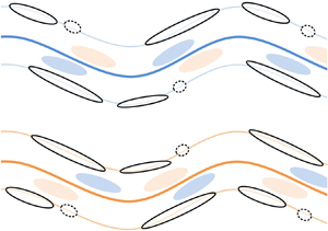


1. Introduction
Energy transfer in both scale and physical space is one of the central keys to unveil the elusive multiscale nature of turbulent flows. Ever since the seminal work of Kolmogorov (Reference Kolmogorov1941), knowledge has been accumulated on how turbulent kinematic energy is redistributed among the scale space to form the so-called direct and inverse energy cascade in homogeneous and isotropic turbulence (known as HIT), e.g. see Biferale (Reference Biferale2003) and Boffetta & Ecke (Reference Boffetta and Ecke2012) for a thorough review. However, as summarized by Alexakisa & Biferale (Reference Alexakisa and Biferale2018), many turbulent flows deviate from homogeneous and isotropic turbulence by much more complicated energy transfer scenarios. In the present study, we will focus on wall-bounded turbulence due to its technological importance. Despite the simple geometry and the absence of intricate forcing conditions, the nature of multidimensionality, inhomogeneity and anisotropy still makes it rather challenging for an ultimate description of the energy transfer and redistribution process in wall-bounded turbulence (Jiménez Reference Jiménez2012).
One of the compromises is to invoke the assumption of local equilibrium in both physical space and scale space. The concept of locality describes that in the overlap (logarithmic) layer intermediate between the inner layer and the outer region, most of the turbulent kinetic energy (TKE) is dissipated at the same wall distance at which it is produced (Jiménez Reference Jiménez2012; Cho, Hwang & Choi Reference Cho, Hwang and Choi2018); meanwhile, interactions between eddies of comparable sizes contribute a remarkable portion of the total scale-energy transfer (Dunn & Morrison Reference Dunn and Morrison2003). Nevertheless, this assumption is somehow challenged by the contemporary knowledge on multiscale coherent structures.
1.1. Energy transfer related to coherent structures
Piomelli et al. (Reference Piomelli, Cabot, Moin and Lee1991) may be one of the first to study the instantaneous scale-energy transfer events in wall-bounded turbulence via an a priori test. The velocity fields of a turbulent channel flow (known as TCF), obtained by direct numerical simulation (DNS), were decomposed into components with resolved scales and unresolved subgrid scales (SGS), respectively. The SGS dissipation term in the evolution equation for the total resolved energy,  $\varepsilon _{SGS}=-\tau _{ij} \partial \tilde {u}_i/\partial x_j$, with
 $\tau _{ij}$ being the subgrid stress tensor and
 $\tilde {u}_i$ the filtered velocity, was analysed to characterize the energy interchange between resolved and SGS scales. It was found that backward scatter events are comparable with forward scatter events in both population density and strength, and the mutual cancellation leads to a net energy flux with magnitude much smaller than that of backward/forward scatter. Here, the term ‘forward scatter’ indicates an energy drain from resolved scales to SGS scales, and vice versa for backward scatter (Kraichnan Reference Kraichnan1976; Leslie & Quarini Reference Leslie and Quarini1979). This seminal work stimulated the following studies attempting to correlate SGS energy transfer with turbulent coherent structures.
Using a similar methodology, together with the technique of conditional averaging, Härtle et al. (Reference Härtle, Klesier, Unger and Friedrich1994) showed that in the buffer layer of a turbulent channel, the bursting events significantly contribute to backward scatter by enforcing the alignment of SGS stresses with the mean rate of strain. Piomelli, Yu & Adrian (Reference Piomelli, Yu and Adrian1996) and Natrajan & Christensen (Reference Natrajan and Christensen2006) analysed the volumetric three-dimensional (3-D) velocity fields of a DNS turbulent channel flow and the streamwise–wall-normal plane of a turbulent boundary layer (TBL) measured by two-dimensional (2-D) particle image velocimetry (PIV), respectively. These two studies suggest a strong spatial coherence between forward and backward scatter events, both of which are related to coherent structures whose conditional-averaged geometries are compatible with the model of hairpin-like vortex or hairpin packet (Adrian Reference Adrian2007). More specifically, the most intense forward scatter events were found to occur where sweep and ejection converge with each other, while backward scatter events were related to diverging sweep and ejection pairs. Similar observations were also reported in the numerical/experimental studies of the SGS energy transfer in convective planetary boundary layer (Lin Reference Lin1999), atmospheric surface layer (Carper & Porté-Agel Reference Carper and Porté-Agel2004) and rough-wall TBL (Hong et al. Reference Hong, Joseph, Charles and Schultz2012). Dong et al. (Reference Dong, Huang, Yuan and Lozano-Durán2020) recently provided a novel 3-D view on the conditional-averaged vortical structure associated with active SGS energy transfer in a homogeneous shear turbulence, in which a pair of streamwise-aligned inverted hairpin and upright hairpin clamp the intense forward or backward scatter in the middle.
Based on these studies, several essential features of the SGS energy transfer in wall-bounded turbulence can be clarified now. Firstly, forward and backward scatter are highly coherent, compact and intermittent. Intense energy transfer events occupying only a small fraction of the space volume were seen to contribute a considerable portion of the total energy flux (Piomelli et al. Reference Piomelli, Yu and Adrian1996; Hong et al. Reference Hong, Joseph, Charles and Schultz2012). This forms the need to study the SGS energy transfer in a structural view. Secondly, the spatial correlation between vortical structures and instantaneous energy flux is non-trivial (Natrajan & Christensen Reference Natrajan and Christensen2006; Hong et al. Reference Hong, Joseph, Charles and Schultz2012; Dong et al. Reference Dong, Huang, Yuan and Lozano-Durán2020). The preferential pairing of intense forward and backward scatter events, which were also observed in 2-D turbulent flows (Liao & Ouellette Reference Liao and Ouellette2013; Fang & Ouellette Reference Fang and Ouellette2016; Zhou et al. Reference Zhou, Huang, Lu, Liu and Ni2016), suggests an intricate alignment between the SGS stress tensor and the resolved rate of strain. It complicates the traditional viewpoint that attributes the forward cascade to the stretching and intensification of vortices by turbulent strain (Tennekes & Lumley Reference Tennekes and Lumley1972). Lastly, the SGS energy flux is usually displaced from the high TKE region (Hong et al. Reference Hong, Joseph, Charles and Schultz2012). This observation implicitly infers the non-negligible contribution of the spatial flux along the inhomogeneous wall-normal direction. As a consequence, the local equilibrium of the in-plane energy cascade might be ‘disrupted’ to some extent.
The last aspect has been addressed by Cimarelli and his colleagues (Cimarelli, De Angelis & Casciola Reference Cimarelli, De Angelis and Casciola2013; Cimarelli et al. Reference Cimarelli, De Angelis, Schlatter, Brethouwer, Talamelli and Casciola2015, Reference Cimarelli, De Angelis, Jiménez and Casciola2016) via analysing the generalized Kolmogorov equation of the second-order velocity structure function. Two scale energy sources, residing in the buffer layer and overlap layer, respectively, are identified, and a complex energy redistribution process, in which attached and detached motions jointly contribute to the coexisting direct and reverse cascades in a spatially evolving way, were derived. This primary finding reminds us of the important role of attached/detached motions on the energy transfer process, which is rather intuitive since these motions dominantly characterize the energy content from intermediate scale to very large-scale and contribute to the interaction between different flow layers (Marusic, Mathis & Hutchins Reference Marusic, Mathis and Hutchins2010; Marusic & Monty Reference Marusic and Monty2019).
In fact, Lin (Reference Lin1999) has already shown that forward scatter events conditioned on positive vertical fluctuating velocity are physically associated with large-scale elongated updrafts, which in a contemporary view are actually large-scale motions (LSMs) or very large-scale motions (VLSMs) (Smits, Mckeon & Marusic Reference Smits, Mckeon and Marusic2011). Lee & Moser (Reference Lee and Moser2019) recently performed a systematic spectral analysis on the TKE budget in a turbulent channel flow with frictional Reynolds number up to  $Re_{\tau }=5200$. They found that VLSMs transfer TKE from streamwise-elongated modes to small-scale ones in a quasi-isotropic way. Meanwhile, the route of the vertical energy transfer resembles those observed by Mizuno (Reference Mizuno2016) and Cimarelli et al. (Reference Cimarelli, De Angelis and Casciola2013, Reference Cimarelli, De Angelis, Schlatter, Brethouwer, Talamelli and Casciola2015, Reference Cimarelli, De Angelis, Jiménez and Casciola2016). Namely, VLSMs drive TKE from the outer region towards the wall to modulate the autonomous near-wall dynamics, while self-similar energy flux structures in the overlap region transport energy away from the wall. Such a picture is also in accordance with the observation of Cho et al. (Reference Cho, Hwang and Choi2018) on the triadic wave interaction of the turbulent transport term in one-dimensional (1-D) spanwise spectral space.
1.2. Aims of the present work and considerations on the methodology
Compared with the steady growing knowledge on the kinematics, dynamics and self-sustaining mechanisms of LSMs and VLSMs, e.g. see Jiménez (Reference Jiménez2018) for a recent update of the list of related literatures, less attention has been paid to the interscale energy transfer and spatial energy transportation that are directly related to LSMs/VLSMs. One of the reasons, to our minds, is that an a priori test of large eddy simulation (known as LES) models only concerns the energy transfer behaviour in the SGS-scale regime. Nevertheless, since these energy-bearing structures seem to be in the central position of the autonomous cycle of the outer region (Hwang & Cossu Reference Hwang and Cossu2010; de Giovanetti, Sung & Hwang Reference de Giovanetti, Sung and Hwang2017), addressing their energy transfer behaviour is still of fundamental importance.
In this background, the present work aims at delineating the characteristics of in-plane energy transfer that is tightly related to LSMs in a structural view. The 2-D velocity fields in wall-parallel planes of a TBL with  $Re_{\tau }=1200\text {--}3500$, that were measured by 2-D PIV at large field-of-view (FOV), were used to perform an a priori test. Due to the 2-D nature of the planar velocity fields, the in-plane energy transfer considered here only takes into account the streamwise and spanwise velocity components and their wall-parallel gradients. This is of course a truncation of the full-order energy transfer term. Nevertheless, a comparison with a DNS dataset obtained by Sillero, Jiménez & Moser (Reference Sillero, Jiménez and Moser2013, Reference Sillero, Jiménez and Moser2014), in which all three velocity components were well resolved, will be made in the following. It will be shown that the essential feature of the large-scale in-plane energy transfer can be well characterized by the present 2-D approximation.
The wall-parallel investigation seems to be another limitation, since the planar dataset excludes the possibility of exploring the vertical energy flux, which has been inferred to play a crucial role in the inner–outer layer interaction (Mathis, Hutchins & Marusic Reference Mathis, Hutchins and Marusic2011; Cimarelli et al. Reference Cimarelli, De Angelis, Schlatter, Brethouwer, Talamelli and Casciola2015); but this is the first step towards a volumetric description. The advantage, to our minds, is the avoidance of the ‘tricky’ issue of inhomogeneity, so that a spectral analysis can be performed along two homogeneous directions, as have been done in Mizuno (Reference Mizuno2016), Chandran et al. (Reference Chandran, Baidya, Monty and Marusic2017) and Lee & Moser (Reference Lee and Moser2019). This approach is also justified by other studies on scale interaction, such as Cimarelli et al. (Reference Cimarelli, De Angelis, Jiménez and Casciola2016) and McKeon (Reference McKeon2017), in which the wall-normal gradient terms are handled separately from those that can be transformed into streamwise–spanwise scale space.
For an a priori test of energy transfer behaviour, the preliminary issue is to divide the scale space into ‘resolved’ and ‘unresolved’ parts. Due to the strong inhomogeneity and anisotropy of LSMs (Chandran et al. Reference Chandran, Baidya, Monty and Marusic2017; Kevin, Monty & Hutchins Reference Kevin, Monty and Hutchins2019), 2-D or 3-D isotropic filters, which were commonly used to separate small scales from large ones (Xiao et al. Reference Xiao, Wan, Chen and Eyink2009; Wang et al. Reference Wang, Wan, Chen and Chen2018a; Motoori & Goto Reference Motoori and Goto2019; Dong et al. Reference Dong, Huang, Yuan and Lozano-Durán2020), cannot be applied here. In the present work, we will use an anisotropic 2-D filter for scale separation. This filter is based on an ‘optimal’ energy flux boundary, across which the maximum energy flux occurs. As will be shown later, it is self-similar in the overlap layer and completely encompasses the energy-bearing large-scale modes.
Finally, the statistical flow structures associated with energy flux events will be obtained under different velocity gradient conditions. The key concept is to break the statistical symmetry along the spanwise direction, which has not been taken into account in previous studies (Piomelli et al. Reference Piomelli, Yu and Adrian1996; Natrajan & Christensen Reference Natrajan and Christensen2006; Hong et al. Reference Hong, Joseph, Charles and Schultz2012; Dong et al. Reference Dong, Huang, Yuan and Lozano-Durán2020). Recently, Kevin et al. (Reference Kevin, Monty and Hutchins2019) have clarified the significance of the meandering motion of LSMs/VLSMs in the log layer and above. Our analysis will demonstrate that the wavy pattern of LSMs, other than streamwise aligned sweep and ejection motions (Natrajan & Christensen Reference Natrajan and Christensen2006), contribute a significant portion of the interscale energy transfer. Meanwhile, the in-plane energy transportation is also tightly related to the asymmetric geometries of LSMs.
The structure of this paper is as follows. The details of the 2-D PIV measurement, as well as the supplemented DNS dataset, are described in § 2. Section 3 deals with the construction of the related anisotropic scale filter via the ‘optimal’ energy flux boundary. The statistics of interscale energy transfer and in-plane energy transportation, together with the conditional-averaged flow field structures, will be presented in §§ 4 and 5, respectively. A conceptual model relating large-scale energy transfer events to LSMs will be formulated in § 6 with some concluding remarks.
2. Experimental set-up
The present experiment was conducted in a low-speed water tunnel in Beihang University, whose main test section has a size of  $18\ \textrm {m} \times 1.2\ \textrm {m} \times 1\ \textrm {m}$ (
 $\textrm {length}\times \textrm {height}\times \textrm {width}$). The free stream turbulence intensity of this facility is approximately
 $T_u\approx 0.8\,\%$ at a typical free stream velocity of
 $U_{\infty }=0.5\ \textrm {m}\ \textrm {s}^{-1}$. A hydraulic smooth acrylic flat plate with length of 15 m, width of 1 m and thickness of 20 mm was vertically positioned in the main test section, on the surface of which a canonical smooth-wall TBL was developed. The leading edge of this flat plate was shaped into a
 $4\,{:}\,1$ half-ellipse to prevent local flow separation. A tripping wire with a diameter of 3 mm was glued on the working surface at 0.4 m downstream of the leading edge. The measurement station located 12 m further downstream, far enough to neglect the tripping condition (Schlatter & Örlü Reference Schlatter and Örlü2012). Hereinafter, the streamwise, wall-normal and spanwise direction are denoted as
 $x$,
 $y$ and
 $z$, respectively. The corresponding instantaneous velocities are
 $U$,
 $V$ and
 $W$ and the fluctuating components are
 $u$,
 $v$ and
 $w$. The superscript
 $(\cdot )^+$ represents a normalization by the frictional velocity
 $u_{\tau }$ or the viscous length scale
 $\nu /u_{\tau }$, and the overline
 $\bar {(\cdot )}$ indicates an ensemble average.
By varying the free stream velocity ( $U_{\infty }=0.15$, 0.34 and
 $0.52\ \textrm {m}\ \textrm {s}^{-1}$), three frictional Reynolds number, i.e.
 $Re_{\tau }=u_{\tau } \delta /\nu \approx 1200$, 2400 and 3500, were tested. They are indicated as case
 $E1\text {--}E3$. Figure 1 shows the wall-normal profiles of both the mean streamwise velocity
 ${\bar {U}^ + }( {{y^ + }} )$ and the streamwise velocity fluctuating intensity
 $\sigma _u^ + ( {{y^ + }} )$, which were measured by a 1-D laser Doppler anemometry (LDA) (Dantec Flow Explorer, Dantec, Denmark) with a probing diameter of 1.0 mm. Existing results of
 $\sigma _u^ + ( {y^ + } )$ obtained by Sillero et al. (Reference Sillero, Jiménez and Moser2013) (via DNS) and
Osaka, Kameda & Mochizuki (Reference Osaka, Kameda and Mochizuki1998), Hultmark et al. (Reference Hultmark, Vallikivi, Bailey and Smits2013) and Willert et al. (Reference Willert, Cuvier, Foucaut, Klinner, Stanislas, Laval, Srinath, Soria, Amili and Atkinson2018) (via experimental measurement) at similar
 $Re_{\tau }$ are superimposed in figure 1(b) for a comparison. Owing to the insufficient resolution of the LDA, the inner peak is slightly underestimated, but
 $\sigma _u^ + ( {y^ + } )$ in the buffer region and above agrees with those of previous studies within the measurement uncertainty. Table 1 summarizes the characteristic parameters of the TBLs, in which the local boundary layer thickness
 $\delta$, the frictional velocity
 $u_{\tau }$ and the shape factor
 $H$ were estimated by fitting the measured
 ${\bar {U}}( {{y}} )$ profiles to the classical formulation of the composite velocity profile (Chauhan, Monkewitz & Nagib Reference Chauhan, Monkewitz and Nagib2009).
Wall-normal profiles of  $(a)$ mean streamwise velocity and
 $(b)$ streamwise fluctuating intensity. Solid markers are obtained by LDA measurements and hollow markers by plan-view PIV. Bold solid lines in panel (a,b) are profiles of DNS data of Sillero et al. (Reference Sillero, Jiménez and Moser2013, Reference Sillero, Jiménez and Moser2014). Dashed lines in panel
 $(a)$ represent the linear law and the logarithmic law, respectively. Dashed lines, dotted lines and dash-dotted lines in panel
 $(b)$ represent the experimental results of Osaka et al. (Reference Osaka, Kameda and Mochizuki1998), Hultmark et al. (Reference Hultmark, Vallikivi, Bailey and Smits2013) and Willert et al. (Reference Willert, Cuvier, Foucaut, Klinner, Stanislas, Laval, Srinath, Soria, Amili and Atkinson2018), respectively.

Characteristic parameters of the experimental and DNS TBLs studied here.

For each experiment case, 2-D PIV measurements were conducted in the wall-parallel planes at four wall-normal heights, i.e.  $y/\delta \approx 0.03$, 0.06, 0.12 and 0.24. With the lower and upper bounds of the log layer being estimated as
 $y^+=3\sqrt {Re_{\tau }}$ and
 $y/\delta =0.15$, respectively (Klewicki, Fife & Wei Reference Klewicki, Fife and Wei2009; Marusic et al. Reference Marusic, Monty, Hultmark and Smits2013), these wall-parallel planes spread from the upper bound of the buffer layer to the lower part of the wake region. Eight synchronized CCD cameras (Imperx ICL-B2520M, Imperx, USA) amounted with Nikkor 50 mm f/1.8D lens were arranged into a
 $4\times 2$ array to cover a FOV of
 $\Delta X\times \Delta Z=636\times 268\ \textrm {mm}^2$, equivalent to
 $3.2\delta \times 1.4\delta$ for case
 $E1$ and
 $3.8\delta \times 1.6\delta$ for cases
 $E2$ and
 $E3$. Each camera had a resolution of
 $2456\times 2048$ pixels and an optical magnification of approximately
 $0.0675\ \textrm {mm}\ \textrm {pixels}^{-1}$. The spatial calibration of the imaging system was taken by fitting second-order polynomials to the images of a customized grid-pattern calibration plate with a size of
 $1\times 0.4\ \textrm {m}$. The FOV of neighbouring cameras had an overlap of 10 mm to facilitate the velocity-field stitching in the post-process stage. As will be demonstrated by both the instantaneous velocity fields in § 4.1 and the 2-D spectrum in figure 2, no velocity discontinuity is seen in the overlapped FOV of neighbouring cameras. Note that such a multicamera PIV configuration has been adopted by Cuvier et al. (Reference Cuvier, Srinath, Stanislas, Foucaut, Laval, Kähler, Hain, Scharnowski, Schröder and Geisler2017) and de Silva et al. (Reference de Silva, Gnanamanickam, Atkinson, Buchmann, Hutchins, Soria and Marusic2014, Reference de Silva, Kevin, Baidya, Hutchins and Marusic2018, Reference de Silva, Chandran, Baidya, Hutchins and Marusic2020) in their studies on large-scale turbulent structures in high
 $Re$ regime. These well-conducted experiments have demonstrated the feasibility of large FOV planar PIV in revealing the multiscale characteristics of wall-bounded turbulence.
Comparison of the premultiplied 2-D spectra of the in-plane fluctuating velocity components at  $y/\delta \approx 0.12$ of all the studied cases:
 $(a)$
 $k_xk_z\varPhi _{uu}(\lambda _x/\delta ,\lambda _z/\delta )$;
 $(b)$
 $k_xk_z\varPhi _{ww}(\lambda _x/\delta ,\lambda _z/\delta )$. Here,
 $\varPhi _{uu|ww}$ are normalized by their individual peak value
 $\varPhi _{max}$. In panel (a,b), solid contour is for case
 $E1$, dotted contour for case
 $E2$, dashed contour for case
 $E3$ and colourmap for case
 $D1$. The contour levels are from 0.1 to 0.85 with a gap of 0.15. Solid straight line denotes
 $\lambda _x=\lambda _z$ and dashed straight line is
 $\lambda _x=\lambda _z^2/5$. The ‘optimal’ boundary
 $B$ to be discussed in figure 3(a) is superimposed as a bold solid curve in panel (a).

Hollow glass beads with a median diameter of  $10\ \mathrm {\mu }\textrm {m}$ and a density of
 $1.05\ \textrm {g}\ \textrm {mm}^{-3}$ were used as seeding particles. The illuminating laser sheet had a thickness of around 1 mm. It was emitted from a double-pulsed Nd:YAG laser generator (Beamtech Vlite-500, Beamtech, China) with energy output of
 $500\ \textrm {mJ}\ \textrm {pulse}^{-1}$, and was directed toward upstream by a reflective mirror being positioned 0.8 m downstream of the end of the FOV. Details about the special treatment of the optical lens to maintain the desired laser-sheet thickness over a relative large streamwise span and the precise positioning of the laser sheet along wall-parallel planes, as well as the minor favourable pressure gradient condition due to the long developing distance of the TBL, can be found in Wang, Pan & Wang (Reference Wang, Pan and Wang2018b). In each case, 3600 pairs of particle images were recorded at a repetition rate of 5 Hz, corresponding to a normalized sampling duration of
 $TU_{\infty }/\delta \approx 530\text {--}2200$ or an eddy turnover time of
 $Tu_{\tau }/\delta \approx 21.2\text {--}84.6$.
The 2-D in-plane velocity fields were calculated from particle image pairs via a graphics processing unit (GPU) accelerated optical flow solver based on Lucas–Kanade algorithm (Pan et al. Reference Pan, Xue, Xu, Wang and Wei2015). The nominal interrogation window was  $48\times 48$ pixels, corresponding to a spatial resolution of
 $12\text {--}32$ wall units/velocity vector. With the maximum straddle-image particle offset being kept as 14–16 pixels in the image plane, the relative error of the velocity measurement was estimated to be around 1 %. The Kolmogorov length scale in the log layer is estimated as
 $\eta ^+=(\kappa y^+)^{1/4}$ (Stanislas, Perret & Foucaut Reference Stanislas, Perret and Foucaut2008). The PIV resolution is approximately
 $5\text {--}9\eta$/velocity vector at
 $y/\delta \approx 0.12$ and relaxes to
 $4\text {--}7\eta$/velocity vector at
 $y/\delta \approx 0.24$. Although the dissipation scale is not well resolved, the present spatial resolution is comparable to several recent multicamera PIV measurements (de Silva et al. Reference de Silva, Gnanamanickam, Atkinson, Buchmann, Hutchins, Soria and Marusic2014, Reference de Silva, Kevin, Baidya, Hutchins and Marusic2018; Cuvier et al. Reference Cuvier, Srinath, Stanislas, Foucaut, Laval, Kähler, Hain, Scharnowski, Schröder and Geisler2017; Zhu et al. Reference Zhu, Lee, Chen, Wu, Chen and Gad-el-Hak2018). On considering the fact that the minimum scale ‘optimal’ energy flux boundary is far beyond
 $\eta$ (to be presented in § 3), the PIV resolution is adequate for the current research purpose of addressing energy transfer associated with large scales. On the other hand, the thickness of the laser sheet is approximately
 $2\text {--}5\eta$ (
 $6\text {--}20$ wall units), two orders smaller than the boundary layer thickness. Furthermore, the laser sheet is placed beyond the upper bound of the buffer layer, where the wall-normal gradient of both
 $\bar {U}$ and
 $\sigma _u$ is insignificant if compared with that in the vicinity of the wall (see figure 1 for illustration). Therefore, the effect of the wall-normal averaging across the laser sheet thickness is regarded as mild.
Owing to the large FOV, each PIV frame contains approximately  $1\times 10^5$ velocity vectors. The variation of local
 $\bar {U}$ and
 ${\sigma _u}$ within a streamwise span of
 $3.8\delta$ is less than
 $5\,\%$. This infers the quasi-parallel (and in-plane homogeneity) condition of the mean flow for the present FOV. Recalling that de Silva et al. (Reference de Silva, Gnanamanickam, Atkinson, Buchmann, Hutchins, Soria and Marusic2014) used 1650 side-view snapshots, each of which contained
 $1.5\times 10^6$ velocity vectors, for statistical analysis, while Cuvier et al. (Reference Cuvier, Srinath, Stanislas, Foucaut, Laval, Kähler, Hain, Scharnowski, Schröder and Geisler2017) acquired 30 000 side-view velocity fields with
 $5.5\times 10^5$ instantaneous vectors in their measurement of a TBL under adverse pressure gradient. In the present work, each experimental case contains 3600 plan-view frames, the total velocity vectors at each flow layer is
 $3.6\times 10^8$, all of which are used for statistical analysis. It has been checked that the convergence of the third-order moments of
 $u$ and
 $w$ can be roughly achieved via 1000 statistical independent frames. An estimation of the uncertainty of the third-order statistics by bootstrap analysis, following the procedure proposed by Hong, Katz & Schultz (Reference Hong, Katz and Schultz2011), is approximately
 $5\,\%$ at a confidence level of
 $95\,\%$ for the whole dataset ensemble. As shown in figure 1, the yielded
 $\bar {U}$ and
 ${\sigma _u}$ at the middle
 $x$ station of the FOV presents reasonable agreement with the LDA results. Moreover, as will be shown in § 3.2, the probability density function (p.d.f.) of the energy transfer events of the PIV case collapses well with that of the reference DNS case, which further verifies that the quality of the present PIV dataset is adequate to address the statistics and characteristics of energy transfer events that are associated with LSMs.
A DNS database of a spatially developing TBL with zero pressure gradient (known as ZPG) is used as a supplementation. It was obtained by Sillero et al. (Reference Sillero, Jiménez and Moser2013, Reference Sillero, Jiménez and Moser2014), and serves as a benchmark for 2-D truncated experiment cases by providing an access to full-order velocity gradient tensors. However, it is noted that the DNS case has a comparably lower Reynolds number. Here, 29 volumetric velocity fields in this database were tailored into an ensemble of 232 smaller volumes with a size of  $\Delta X\times \Delta Y\times \Delta Z=4\delta \times \delta \times 2\delta$, in the middle of which the nominal Reynolds number is
 $Re_{\tau }=1750$. This dataset is denoted as case
 $D1$. Its characteristic boundary layer parameters are listed in table 1, and the corresponding
 $\bar {U}$ and
 ${\sigma _u}$ profiles are shown in figure 1.
Figure 2 compares the premultiplied 2-D spectra of  $u$ and
 $w$, i.e.
 $k_xk_z\varPhi _{uu}(\lambda _x/\delta ,\lambda _z/\delta )$ and
 $k_xk_z\varPhi _{ww}(\lambda _x/\delta ,\lambda _z/\delta )$, at
 $y/\delta \approx 0.12$ of all the studied cases (case
 $E1\text {--}E3$ and case
 $D1$). The spectra of streamwise and spanwise velocity,
 $\varPhi _{uu}$ and
 $\varPhi _{ww}$, are defined as
 $\langle \hat {u} \hat {u}^* \rangle$ and
 $\langle \hat {w} \hat {w}^* \rangle$, where
 $\hat {u}$ and
 $\hat {w}$ are 2-D Fourier transform of
 $u(x,z)$ and
 $w(x,z)$. Note that both spectra are calculated from in-plane fields without invoking Taylor's hypothesis. In general, the outer-scaled
 $k_xk_z\varPhi _{uu}$ and
 $k_xk_z\varPhi _{ww}$ are less sensitive to
 $Re_{\tau }$ in the intermediate scale of
 $\lambda _x\approx 0.2\delta \sim \delta$ and
 $\lambda _z\approx 0.1\text {--}0.5\delta$. This observation provides a justification for the accuracy of the present PIV measurement. The slight offset of the spectral peak in the experiment contours from the DNS ones is attributed to both the insufficient resolution of larger scales (
 $\lambda _x>3\delta$) and the different tripping conditions. The scaling of
 $\lambda _x=\lambda _z$ (bold solid lines in figure 2) and
 $\lambda _x=\lambda _z^2/5$ (bold dashed lines) clamp the plateau region of the
 $k_xk_z\varPhi _{uu}$ spectra in between, similar to the observation in del Álamo et al. (Reference del Álamo, Jiménez, Zandonade and Moser2004). The linear scaling of
 $\lambda _x=\lambda _z$ also well characterizes the ridges of the
 $k_xk_z\varPhi _{ww}$ spectra, which indicates a constant aspect ratio of the energy-bearing
 $w$ modes. This is consistent with the so-called
 $y$-scaling law of 1-D spectrum of wall-parallel velocity components (Agostini & Leschziner Reference Agostini and Leschziner2017; Baars, Hutchins & Marusic Reference Baars, Hutchins and Marusic2017) that are believed to be attributed by wall-attached eddies. Due to the limited FOV (
 $\Delta X=3.2\text {--}3.8\delta$), scales associated with VLSMs are not fully resolved in case
 $E1\text {--}E3$. This is a practical limitation when obtaining a 2-D spectrum via PIV measurement. Nevertheless, it is stressed that the ‘optimal’ energy flux boundary (bold yellow lines in figure 2, to be explained in § 3) is on the small-scale side of the energy peak of
 $k_xk_z\varPhi _{uu}$. Therefore, the energy flux across this boundary is expected to be less sensitive to structures larger than the extent of FOV. This issue will be further addressed in appendix C by evaluating the DNS dataset truncated at various FOV.
3. Scale decomposition for energy transfer related to LSMs
3.1. ‘Optimal’ spectral energy flux boundary
Most of the previous studies used a small-scale isotropic filter ( $\lambda ^+_{x|y|z}\sim O(10^2)$) for scale separation (Piomelli et al. Reference Piomelli, Yu and Adrian1996; Natrajan & Christensen Reference Natrajan and Christensen2006; Dong et al. Reference Dong, Huang, Yuan and Lozano-Durán2020). This is not suitable for the purpose of investigating the energy transfer behaviour associated with larger-scale structures. Therefore, we revisit the inertial energy transfer term in the evolution equation of TKE in shear flows, whose formulation in spectral space is
 \begin{align} & \frac{{\partial \varPhi \left( {{k_x},{k_z},y} \right)}}{{\partial t}} = - \underbrace{\left\langle {{{\hat{u}}^*}\hat{v} + \hat{u}{{\hat{v}}^*}} \right\rangle \frac{{\textrm{{d}}\langle U\rangle }}{{2\textrm{{d}}y}}}_{\hat{P}} \underbrace{-\frac{1}{2}\left\langle {\hat{u}_i^*\widehat{\frac{{\partial {u_i}{u_j}}}{{\partial {x_j}}}} + {{\hat{u}}_i}{{\widehat{\frac{{\partial {u_i}{u_j}}}{{\partial {x_j}}}}}^*}} \right\rangle }_{\hat{T}} \nonumber\\ &\quad - \underbrace{\left\langle {\frac{\textrm{{d}}}{{\textrm{{d}}y}}\left( {\frac{{\hat{p}{{\hat{v}}^*} + {{\hat{p}}^*}\hat{v}}}{2\rho }} \right)} \right\rangle }_{{{\hat{T}}_p}}+ \underbrace{\nu \left\langle {\frac{{{\textrm{{d}}^2}\varPhi }}{{\textrm{{d}}{y^2}}}} \right\rangle }_{{{\hat{T}}_{\nu} }} - \underbrace{\frac{\nu}{2} \left\langle {{{\widehat{\frac{{\partial {u_i}}}{{\partial {x_j}}}}}^*}\widehat{\frac{{\partial {u_i}}}{{\partial {x_j}}}} +\widehat{\frac{{\partial {u_i}}}{{\partial {x_j}}}}{{\widehat{\frac{{\partial {u_i}}}{{\partial {x_j}}}}}^*}} \right\rangle }_{\hat{\varepsilon}}. \end{align}
This formulation can be derived by applying a 2-D Fourier transform to the evolution equation of the in-plane two-point velocity correlation function for shear flows (Monin & Yaglom Reference Monin and Yaglom1975). In (3.1),  $\varPhi$ is the spectral TKE, i.e. the density of TKE at a set of wavenumbers (
 $k_x$,
 $k_z$) and a particular flow layer of
 $y$,
 $\hat {(\cdot )}$ indicates a variable in 2-D spectral space with the dependent variables
 $k_x$,
 $k_z$ and
 $y$ being omitted,
 $(\cdot )^*$ is the complex conjugate and
 $\langle \cdot \rangle$ denotes an ensemble average. On the right-hand side of (3.1),
 $\hat {P}$ is the turbulence production term,
 $\hat {T}$ is the inertial transfer term caused by turbulent convection,
 $\hat {T}_p$ is the fluctuation-pressure interaction term, and
 $\hat {T}_{\nu }$ or
 $\hat {\varepsilon }$ are the viscous diffusion or dissipation term, respectively.
Note that  $\hat {T}$ is the only term that exclusively includes the effect of turbulent fluctuation. It is actually a summation of nine components, i.e.
 \begin{equation} \hat{T}\left( {{k_x},{k_z}} \right)= \sum_{i,j = 1}^3 {{{\hat{T}}_{ij}}\left( {{k_x},{k_z}} \right)}. \end{equation}
For the present wall-parallel dataset, only four components with  $i$,
 $j=1$ and 3 are kept. This enables us to reformulate
 ${{\hat {T}}_{ij}}$ in a sense of triadic interaction between three wavenumbers
 $k$,
 $k'$ and
 $k-k'$ (Monin & Yaglom Reference Monin and Yaglom1975), i.e.
 \begin{equation} {{\hat{T}}_{ij}}({k_x},{k_z}) =\mathrm{Re}\left\langle \sum_{{k_x'},{k_z'}} {\mathrm{i}{k_j}{\hat{u}_i^*( {{k_x},{{k}_z}} )\hat{u}_j( {{k_x} - {{k}_x'},{k_z} - {{k}_z'}} ){{\hat{u}}_i}( {{k_x'},{k_z'}} )} } \right\rangle, \quad i,j \in \{1,3\}. \end{equation}
Such a formulation implies that the exchange of scale energy in a wall-parallel plane by turbulent motion is embodied as the energy flux due to triadic-wave interaction, similar to the scenario in homogeneous and isotropic turbulence (Cardesa, Vela-Martín & Jiménez Reference Cardesa, Vela-Martín and Jiménez2017). Note that this form cannot be obtained if the components associated with the vertical gradient (with  $j=2$) in (3.2) are included.
Here, we define the in-plane energy transfer term as
 \begin{equation} {\hat{T}_{XZ}({k_x},{k_z})} = \sum_{i,j} {{{\hat{T}}_{ij}}({k_x},{k_z})}, \quad i,j \in \{1,3\}, \end{equation}
which measures the rate of change of the spectral TKE (without  $v$ component) owing to
 $u$ and
 $w$ component turbulent fluctuations in the
 $x$–
 $z$ plane. The spectra of
 ${\hat {T}_{XZ}({k_x},{k_z})}$ present similar patterns among all the studied wall-parallel planes (
 $y/\delta =0.03\text {--}0.24$). One example at
 $y/\delta =0.12$ in case
 $E3$ (with
 $Re_{\tau }=3500$) is given in figure 3(a), which shows that
 ${\hat {T}_{XZ}({k_x},{k_z})}$ is characterized as one positive large-scale patch and one negative small-scale patch divided by a zero-crossing line
 $B$ (bold dashed line in figure 3a). These two patches represent the energy donor modes and energy recipient modes (Lee & Moser Reference Lee and Moser2019), respectively, and are consistent with the formal concept that on average large-scale eddies lose energy, while small-scale fluctuations gain energy.
 $(a)$ In-plane energy transfer spectrum
 ${\hat {T}_{XZ}}(\lambda _x/\delta , \lambda _z/\delta )$ at
 $y/\delta \approx 0.12$ in case
 $E3$. Bold dashed line shows the boundary between the energy donor and energy recipient modes at
 $y/\delta \approx 0.12$, while light dashed lines indicate the corresponding boundaries at other flow layers, i.e.
 $y/\delta \approx 0.03$, 0.06 and 0.24. The solid line
 $C$ is an arbitrary path of the energy transfer.
 $(b)$ Wall-normal variation of the absolute value of the total
 ${\hat {T}_{XZ}}$ or
 $\hat {T}$ integrated over the energy donor or energy recipient modes, which are separated by the zero-crossing boundary
 $B$ shown in panel
 $(a)$. The upper half-plane is for
 $\iint |\hat {T}^{+|-}_{XZ}|\,\textrm {d}k_x\,\textrm {d}k_z$ in case
 $E3$, and the lower half-plane for
 $\iint |\hat {T}^{+|-}|\,\textrm {d}k_x\,\textrm {d}k_z$ in case
 $D1$.

The integration of  ${\hat {T}_{XZ}({k_x},{k_z})}$ in the whole scale space is close to zero for all the investigated flow layers. This can be evidenced by figure 3(b), in which the magnitudes of
 $\iint _{\hat {T}_{XZ}\ge 0}|\hat {T}_{XZ}|\,\textrm {d}k_x\,\textrm {d}k_z$ are almost identical to that of
 $\iint _{\hat {T}_{XZ}<0}|\hat {T}_{XZ}|\,\textrm {d}k_x\,\textrm {d}k_z$. Such an observation seems to be in accordance with the quasi-local assumption of the energy cascade. However, figure 3(b) also shows that when both the
 $v$ component and the vertical gradient are taken into account in the full resolved
 $\hat {T}$, slight imbalance between
 $\iint _{\hat {T}\ge 0}|\hat {T}|\,\textrm {d}k_x\,\textrm {d}k_z$ and
 $\iint _{\hat {T}<0}|\hat {T}|\,\textrm {d}k_x\,\textrm {d}k_z$ appears in the log layer and below of case
 $D1$ (with
 $Re_{\tau }=1750$). This highlights the contribution of the wall-normal turbulent motion on the inertial energy transfer (Cimarelli et al. Reference Cimarelli, De Angelis, Jiménez and Casciola2016; Lee & Moser Reference Lee and Moser2019). Nevertheless, the overall level, as can be estimated by the difference between
 $\iint _{\hat {T}\ge 0}|\hat {T}|\,\textrm {d}k_x\,\textrm {d}k_z$ and
 $\iint _{\hat {T}<0}|\hat {T}|\,\textrm {d}k_x\,\textrm {d}k_z$, is relatively small if compared with that of the in-plane energy transfer. This provides a justification for neglecting the wall-normal energy transfer as a leading-order approximation in the present study.
By superimposing the zero-crossing boundary  $B$ onto the
 $\varPhi _{uu}$ spectrum (in figure 2a), it is clearly seen that the energy-bearing large scales (with spectral peak at
 $\lambda _x\sim 2\delta$ and
 $\lambda _z \sim 0.5\delta$) reside in the positive
 $\hat {T}_{XZ}$ region. This is consistent with previous observations that the spectral peak of the turbulent production term locates inside the energy donor modes (Mizuno Reference Mizuno2016; Cho et al. Reference Cho, Hwang and Choi2018; Lee & Moser Reference Lee and Moser2019). Denoting the minimum streamwise and spanwise length scale of
 $B$ as
 $\lambda ^B_{x0}$ and
 $\lambda ^B_{z0}$, respectively. Figure 3(a) shows that
 $\lambda ^B_{z0}$ in case
 $E3$ increases from
 $0.04\delta$ to
 $0.12\delta$ as the flow layer elevates from
 $y/\delta \approx 0.03\text {--}0.24$; in contrast,
 $\lambda ^B_{x0}$ only varies from 0.15
 $\delta$ to 0.2
 $\delta$. Figure 15 in appendix A further shows that for all the studied cases,
 $\lambda ^B_{z0}/\delta$ is quasi-linearly proportional to
 $y/\delta$ across a wide range of
 $y$, while the variation of
 $\lambda ^B_{x0}/\delta$ in the log layer is mild.
The zero-crossing boundary  $B$ in the
 $\hat {T}_{XZ}$ spectrum is regarded as the ‘optimal’ energy flux boundary, across which the spectral energy flux is maximum. As illustrated in figure 3(a), this can be visualized by drawing an arbitrary path
 $C$ in the 2-D wavenumber space from the origin
 $(0,0)$ to one set of
 $(\kappa _x,\kappa _z)$. The net scale energy transferred from larger scales to
 $(\kappa _x, \kappa _z)$ along
 $C$ is defined as the following curvilinear integral:
 \begin{equation} \hat{\varPi} ({\kappa_x},{\kappa_z}) = \int_{\boldsymbol{r}=(0,0)}^{\boldsymbol{r}=(\kappa_x,\kappa_z)}{ - {{\hat{T}}_{XZ}}\left( {{k_x},{k_z}} \right)}\,\textrm{{d}}\boldsymbol{r}. \end{equation}
It is easy to see that  $\hat \varPi$ reaches a maximum when
 $(\kappa _x, \kappa _z)$ falls on
 $B$. In the following analysis, this ‘optimal’ energy flux boundary is used as the cutting-off threshold of a 2-D sharp-edge filter to separate large-scale modes from smaller ones at each flow layer. The physical significance of such an anisotropic filter is that the yielded net energy exchange is the most intense in an ensemble-averaged sense, as the ‘large’ and ‘small’ scales are actually the energy donor modes or energy recipient modes in the energy transfer spectrum.
3.2. Statistics of energy transfer events
In order to explore the relationship between energy transfer and LSMs, the instantaneous energy transfer event should be properly defined at first. The evolution equation of the ‘resolved’ instantaneous TKE in physical space is
 \begin{equation} \frac{{\partial \tilde{Q}\left( {x,z,y} \right)}}{{\partial t}} = \underbrace{-\tilde{u}\tilde{v}\frac{{\textrm{{d}}\langle U\rangle }}{{\textrm{{d}}y}}}_P \underbrace{-{{\tilde{u}}_i}\frac{{\partial \widetilde{{u_i}{u_j}}}}{{\partial {x_j}}}}_T \underbrace{-\frac{\textrm{{d}}}{{\textrm{{d}}y}}\left( {\frac{{\tilde{p}\tilde{v}}}{\rho }} \right)}_{{T_p}} + \underbrace{\nu \frac{{{\textrm{{d}}^2}\tilde{Q}}}{{\textrm{{d}}{y^2}}}}_{{T_{\nu} }} \underbrace{-\nu \frac{{\partial {{\tilde{u}}_i}}}{{\partial {x_j}}}\frac{{\partial {{\tilde{u}}_i}}}{{\partial {x_j}}}}_{\varepsilon} , \end{equation}
in which  $\tilde {(\cdot )}$ denotes those filtered variables including only ‘resolved’ scales and
 $\tilde {Q}=\tilde {u}_i \tilde {u}_i/2$ (with
 $i=1$, 3) is the ‘resolved’ TKE. The terms on the right-hand side of (3.6) correspond to those in (3.1) in spectral space.
According to Piomelli et al. (Reference Piomelli, Cabot, Moin and Lee1991, Reference Piomelli, Yu and Adrian1996) and Natrajan & Christensen (Reference Natrajan and Christensen2006), the inertial transfer term  $T$ can be decomposed as follows:
 \begin{align} T &=- {\tilde{u}_i}\frac{{\partial\widetilde{{u_i}{u_j}}}}{{\partial {x_j}}} = -\left({\tilde{u}_i}\frac{{\partial {{\tilde{u}}_i}{{\tilde{u}}_j}}}{{\partial {x_j}}}+{\tilde{u}_i}\frac{{\partial (\widetilde{{u_i}{u_j}} - {{\tilde{u}}_i}{{\tilde{u}}_j})}}{{\partial {x_j}}}\right) \nonumber\\ &=-\left(\frac{{\partial {{\tilde{Q}}}{{\tilde{u}}_j}}}{{\partial {x_j}}} +\frac{{\partial {{\tilde{u}}_i}\left( {\widetilde{{u_i}{u_j}} - {{\tilde{u}}_i}{{\tilde{u}}_j}} \right)}}{{\partial {x_j}}} -\left( {\widetilde{{u_i}{u_j}} - {{\tilde{u}}_i}{{\tilde{u}}_j}} \right)\frac{{\partial {{\tilde{u}}_i}}}{{\partial {x_j}}}\right). \end{align}
In (3.7), the first two terms on the second line represent the large-scale and subgrid-scale diffusion terms, respectively, while the third term is essentially the same as the subgrid dissipation term, i.e.  $\varepsilon _{{SGS}}$, that needs to be modelled in large eddy simulations. Recalling that
 $T$ is the instantaneous counterpart of
 $\hat {T}$ being integrated in the large-scale side of the ‘optimal’ energy flux boundary
 $B$; therefore, it accounts for the effect of triadic interaction among all the scales (as shown in (3.3)). However, previous works (Piomelli et al. Reference Piomelli, Yu and Adrian1996; Liao & Ouellette Reference Liao and Ouellette2013) have shown that only those scale interaction forms represented by
 $\varepsilon _{{SGS}}$ are responsible for the net energy exchange between ‘resolved’ and ‘unresolved’ scales, which is the reason that
 $\varepsilon _{{SGS}}$ is named as subgrid energy flux. In contrast, the large-scale and subgrid-scale diffusion terms play a role of redistributing large-scale energy in physical space through turbulent convection.
Following Piomelli et al. (Reference Piomelli, Yu and Adrian1996), we define instantaneous in-plane spatial energy flux as  $\varPi _{{d}}$, instantaneous interscale energy flux as
 $\varPi _{{SGS}}$ and their sum as the total energy flux
 $\varPi$, i.e.
 \begin{gather} \varPi_{{d}} =\sum_{i,j}\left(\frac{{\partial {{\tilde{Q}}}{{\tilde{u}}_j}}}{{\partial {x_j}}}+\frac{{\partial {{\tilde{u}}_i}\left( {\widetilde{{u_i}{u_j}} - {{\tilde{u}}_i}{{\tilde{u}}_j}} \right)}}{{\partial {x_j}}}\right),\quad i,j \in \left\{ {1,3} \right\}, \end{gather}
 \begin{gather} {\varPi_{{SGS}}} =\sum_{i,j} - \left( {\widetilde{{u_i}{u_j}} - {{\tilde{u}}_i}{{\tilde{u}}_j}} \right)\frac{{\partial {{\tilde{u}}_i}}}{{\partial {x_j}}},\quad i,j \in \left\{ {1,3} \right\}, \end{gather}
 \begin{gather} \varPi= \varPi_{{d}} + {\varPi_{{SGS}}}. \end{gather}
Note that the summation convention is not applied in (3.8)–(3.9), and the indexes  $(i,j)$ only account for wall-parallel dimensions. Tests on the DNS dataset given in appendix A show that for the present scale cutting-off boundary, the in-plane components (with
 $i,j\in \{ {1,3} \}$) dominate over the vertical ones (with
 $i$ or
 $j=2$) in the full-resolved
 $\varPi _{{SGS}}$; however, the contribution of the latter becomes non-negligible when a small-scale isotropic filter is used for scale separation (see figure 16). This justifies the experimental attempt of using only in-plane components to characterize interscale energy flux that are associated with energy-bearing scales. On the other hand, the contributions of both in-plane and vertical components to
 $\varPi _{{d}}$ are insensitive to the scale filter (see figure 17).
The p.d.f.s of  $\varPi$,
 $\varPi _{{SGS}}$ and
 $\varPi _{{d}}$ are analysed first. All the studied flow layers have similar p.d.f. distributions; therefore, only the results at
 $y/\delta \approx 0.12$ in case
 $E3$ and case
 $D1$ are illustrated in figure 4. Satisfying collapses are observed between case
 $E3$ and case
 $D1$ when
 $\varPi$,
 $\varPi _{{SGS}}$ and
 $\varPi _{{d}}$ are normalized by their own root mean squared (known as RMS) value. The p.d.f. of
 $\varPi _{{d}}$ (shown in figure 4c) is symmetrical about the origin, indicating a zero net in-plane energy flux, i.e.
 $\langle \varPi _{{d}}\rangle =0$. It demonstrates that
 $\varPi _{{d}}$ does not alter the overall level of energy but only redistributes energy in space, consistent with the homogeneous condition in wall-parallel dimension (when only the in-plane turbulent motion is concerned). In contrast, asymmetry between forward scatter events (with positive
 $\varPi _{{SGS}}$) and backward scatter ones (with negative
 $\varPi _{{SGS}}$) is seen in the p.d.f. of
 $\varPi _{{SGS}}$ (in figure 4b), which is inherited by the p.d.f. of
 $\varPi$ (in figure 4a). The ensemble-averaged
 $\langle \varPi _{{SGS}}\rangle$ and
 $\langle \varPi \rangle$ are both positive, consistent with the formal energy cascade and the fact that ‘resolved’ scales are actually those energy donor modes in the in-plane energy transfer spectrum
 $\hat {T}_{XZ}(k_x, k_z)$.
Premultiplied p.d.f. of (a)  $\varPi$, (b)
 $\varPi _{{SGS}}$ and (c)
 $\varPi _{{d}}$ at
 $y/\delta \approx 0.12$ for both case
 $E3$ (discrete bars) and case
 $D1$ (solid and dashed curves). Positive and negative events are plotted on the same side to highlight the symmetry condition. Owing to the premultiplication, the height of each bar (or curve segment) measures the relative contribution of the corresponding event to the net energy flux.

4. Interscale energy transfer structures
In this section and the next one, the planar flow structures associated with both interscale energy transfer events ( $\varPi _{{SGS}}$) and in-plane energy transportation events (
 $\varPi _{{d}}$) will be explored individually.
4.1. Visualization of  $\varPi _{{SGS}}$ event

Figure 5 plots one snapshot of  $\tilde {u}(x, y)$,
 $\varPi _{{SGS}}(x, y)$ and
 $\varPi _{{d}}(x, y)$ at different flow layers in case
 $E3$ for a qualitative visualization. Hereinafter, only the results of case
 $E3$ are to be presented. appendix D deals with the
 $Re$ effect. It will be shown that for the present studied flow regions, the characteristics of interscale energy transfer and in-plane energy transportation are less dependent on
 $Re$ (with
 $Re_{\tau }=1200 \text {--}3500$).
Instantaneous field of  $\tilde {u}$ (filled contours),
 $\varPi _{{SGS}}$ (isolines in a,c,e,g) and
 $\varPi _{{d}}$ (isolines in b,d,f,h) at (a,b)
 $y/\delta \approx 0.03$, (c,d)
 $y/\delta \approx 0.06$, (e,f)
 $y/\delta \approx 0.12$ and (g,h)
 $y/\delta \approx 0.24$ in case
 $E3$. In panel (a,c,e,g), solid (or dashed) isolines indicate forward (or backward) scatter events with
 $\varPi _{{SGS}}= {\pm}1.5\sigma _{\varPi _{{SGS}}}$, while clusters of forward and backward scatter events are marked by dashed circles, arrows highlight forward scatter events at spanwise interfaces of high- and low-momentum regions, and solid circles highlight those at streamwise interfaces. In panel (b,d,f,h), solid (dashed) isolines indicate positive (or negative) energy transfer events with
 $\varPi _{{d}}={\pm}1.5 \sigma _{\varPi _{{d}}}$, solid circles indicate pairs of
 ${\pm }\varPi _d$ events inside low-momentum LSMs.

As shown in figure 5, streaky-like large-scale  $\tilde {u}$ structures resembling LSMs are evident from the buffer layer to the lower part of the wake region. They are highly sinusoidal in shape, and their spanwise width presents a significant growth with the increase of
 $y$. Note that the size of these typical
 $\tilde {u}$ structures is fairly large compared with the ‘optimal’ energy flux boundary; therefore, their geometries will not be significantly biased by the low-pass sharp-edge filtering.
As for  $\varPi _{{SGS}}$, its distribution is more trivial and chaotic in the near-wall region (in figure 5a), but tends to be more compact and coherent in higher layers (in figure 5e,g). Two types of
 $\varPi _{{SGS}}$ events are seen. Firstly, fragmented regions of
 $\varPi _{{SGS}}$ with alternating sign aggregate into a pattern of staggered cluster (indicated by dashed circles in figure 5c,e,g). A mutual cancellation of
 $\pm \varPi _{{SGS}}$ in the cluster yield only weak (if not zero) net interscale energy flux. Such a pattern is similar to the spinwheel-like pattern of alternating lobes of
 $\pm \varPi _{{SGS}}$ in 2-D turbulence, which were found to be related to strong rotational motions by Liao & Ouellette (Reference Liao and Ouellette2013). Secondly, isolated
 $\varPi _{{SGS}}$ events scatter in the flow field, among which the population density of positive events are distinctly higher than those of negative ones. It is this kind of event that contribute to the asymmetry of the p.d.f. of
 $\varPi _{{SGS}}$.
A careful inspection shows that these isolated  $\varPi _{{SGS}}$ events are highly correlated with intense local velocity gradients along either the spanwise direction or streamwise direction, i.e.
 $\partial \tilde {u}/\partial z$ or
 $\partial \tilde {u}/\partial x$. The former case (arrow-indicated regions in figure 5a,c,e,g) usually appears on the spanwise interface between
 $\pm \tilde {u}$ structures, while the latter case (regions inside solid circles in figure 5e,g) prefers to appear in-between streamwise-aligned
 $\tilde {u}$ structures with alternating sign. Note that the latter case has been seen in the
 $x$–
 $y$ plane by Natrajan & Christensen (Reference Natrajan and Christensen2006), who attributed it to the opposing Q2 and Q4 events induced by hairpin vortices. Nevertheless, the former one, which seems to have higher occurrence probability in the log layer and above, has not been reported before.
4.2. Cumulative spectrum of $\varPi _{{SGS}}$ events

For a quantitative characterization of the above observation, cumulative energy flux  $\sum _{\chi } \varPi _{{SGS}}$ under particular flow conditions, i.e.
 $\chi =\tilde {u}$,
 $\partial \tilde {u}/\partial z$ and
 $\partial \tilde {u}/\partial x$, are shown in figure 6 for case
 $E3$ to evaluate their individual contributions to the net interscale energy flux
 $\langle \varPi _{{{SGS}}}\rangle$. Additionally,
 $\pm \varPi _{{SGS}}$ events are differentiated in the add-up process to indicate their relative contributions. The yielded values are denoted as
 $\sum _{\chi }\varPi ^+_{{SGS}}$ and
 $\sum _{\chi }\varPi ^-_{{SGS}}$, respectively, and are also shown in figure 6. Since
 $\partial {\tilde {w}}/\partial x_j$ are generally smaller than
 $\partial {\tilde {u}}/\partial x_j$, they are removed from the candidate velocity gradient conditions to be examined. Meanwhile, the condition of
 $\tilde {u}$ is reserved to quantify the correlation between
 $\varPi _{{SGS}}$ and LSMs.
The 1-D cumulative spectrum of interscale energy flux  $\sum _{\chi }\varPi _{{{SGS}}}$ with respect to flow conditions
 $\chi$ in case
 $E3$.
 $(a)$
 $\chi =\tilde {u}$,
 $(b)$
 $\chi =\partial \tilde {u}/{\partial z}$ and
 $(c)$
 $\chi ={\partial \tilde {u}}/{\partial x}$. Solid line,
 $y/\delta \approx 0.03$; dashed line,
 $y/\delta \approx 0.06$; dot-dash line,
 $y/\delta \approx 0.12$; and dotted line,
 $y/\delta \approx 0.24$. The group of profiles marked by
 $\varPi ^+_{{SGS}}$,
 $\varPi ^-_{{SGS}}$ or
 $\varPi _{{SGS}}$ represent the cumulative contribution from forward scatter events, backward scatter events or all of the events, respectively. Velocity gradients conditions are normalized by their root mean squared value, the same in the following figures.

Figure 6 leads to several interesting observations. Firstly, the profiles of  $\sum _{\tilde {u}} \varPi _{{SGS}}(\tilde {u})$ (in figure 6a) centre around
 $\tilde {u}=0$ with a slight left-offset. Such an asymmetry is seen to be inherited from that of
 $\sum _{\tilde {u}} \varPi ^+_{{SGS}}(\tilde {u})$ whose peaks locate at
 $\tilde {u}/\sigma _{\tilde {u}}\approx -0.3$. In contrast,
 $\sum _{\tilde {u}} \varPi ^-_{{SGS}}(\tilde {u})$ keeps a satisfying symmetry. The high magnitude of
 $\sum _{\tilde {u}} \varPi ^{\pm }_{{SGS}}$ around
 $\tilde {u}=0$ suggests a weak correlation between the core region of LSMs and
 $\varPi _{{SGS}}$ events. Secondly,
 $\sum _{{\partial \tilde {u}}/{\partial z}} \varPi ^+_{{SGS}}({\partial \tilde {u}}/{\partial z})$ presents a bimodal profile (in figure 6b), except for the highest flow layer (at
 $y/\delta \approx 0.24$) where a plateau, instead of two isolated peaks, appears in the range of
 $({\partial \tilde {u}}/{\partial z})/\sigma ({\partial \tilde {u}}/{\partial z}) \in [-1 , +1]$. This bimodal pattern, together with the skewness of
 $\sum _{\tilde {u}} \varPi ^+_{{SGS}}(\tilde {u})$ towards the
 $+\tilde {u}$ side, provides a statistical support for the preferential alignment of forward scatter events along the flanks of low-momentum LSMs, as has been visualized in figure 5(a,c,e,g) (as arrow-indicated regions). Finally, the profiles of
 $\sum _{{\partial \tilde {u}}/{\partial x}}\varPi _{{SGS}}({\partial \tilde {u}}/{\partial x})$ (in figure 6c) present an asymmetric bimodal pattern with two peaks locating at
 $({\partial \tilde {u}}/{\partial x})/\sigma ({\partial \tilde {u}}/{\partial x})\approx 0.5$ and
 $-1.5$, respectively. This pattern is jointly contributed by quasi-symmetric single-peak profiles of
 $\sum _{{\partial \tilde {u}}/{\partial x}}\varPi ^-_{{SGS}}({\partial \tilde {u}}/{\partial x})$ and negative-skewed profiles of
 $\sum _{{\partial \tilde {u}}/{\partial x}}\varPi ^+_{{SGS}}({\partial \tilde {u}}/{\partial x})$, the latter of which is consistent with the visualization that forward scatter events can be found in the middle of streamwise-aligned positive and negative LSMs (bold solid circles in figure 5e,g) where
 ${\partial \tilde {u}}/{\partial x}<0$.
The dependency of  $\varPi _{{SGS}}$ on both
 ${\partial \tilde {u}}/{\partial x}$ and
 ${\partial \tilde {u}}/{\partial z}$ is further considered by constructing a bivariate cumulative spectrum, i.e.
 $\sum _{\chi }\varPi _{{SGS}}(\chi )$ with
 $\chi =[{{\partial \tilde {u}}/{\partial x}}, {{\partial \tilde {u}}/{\partial z}}]$. Hereinafter,
 $\chi$ is omitted in the 2-D summation operator
 $\sum _{\chi }$ for simplicity. Here,
 $\tilde {u}$ is not regarded as one of the joint conditions due to its weak correlation with
 $\varPi ^{\pm }_{{SGS}}$, as has been shown in the univariate cumulative profiles in figure 6(a). Figure 7 shows
 $\sum \varPi ^{\pm }_{{SGS}}$ and
 $\sum \varPi _{{SGS}}$ in the phase plane of (
 ${{\partial \tilde {u}}/{\partial x}}, {{\partial \tilde {u}}/{\partial z}})$ at
 $y/\delta \approx 0.12$ in case
 $E3$, while figure 19 in appendix D will summarize the cumulative spectra of
 $\sum \varPi _{{SGS}}({{\partial \tilde {u}}/{\partial x}}, {{\partial \tilde {u}}/{\partial z}})$ in all the studied cases to evidence both a
 $Re$-independency and a flow-layer insensitivity.
The 2-D cumulative spectrum of  $(a)$ positive interscale energy flux events
 $\sum \varPi ^+_{{SGS}}$,
 $(b)$ negative events
 $\sum \varPi ^-_{{SGS}}$ and (c) all of the events
 $\sum \varPi _{{SGS}}$ in the phase space of
 $({\partial \tilde {u}}/{\partial x},{\partial \tilde {u}}/{\partial z})$ at
 $y/\delta \approx 0.12$ in case
 $E3$. Each spectrum is normalized by its peak value. The subpartitions marked in panel
 $(c)$ are defined in table 2.

The 2-D contours of both  $\sum \varPi ^+_{{SGS}}$ and
 $\sum \varPi ^-_{{SGS}}$ (in figure 7a,b) are symmetric in the
 ${{\partial \tilde {u}}/{\partial z}}$ dimension but asymmetric in the
 ${{\partial \tilde {u}}/{\partial x}}$ dimension. Two peaks in
 $\sum \varPi ^+_{{SGS}}$ both locate at the
 ${{+\partial \tilde {u}}/{\partial x}}$ side and straddle on each side of the
 ${{\partial \tilde {u}}/{\partial z}}$ axis. In contrast,
 $\sum \varPi ^-_{{SGS}}$ peaks at
 ${{-\partial \tilde {u}}/{\partial x}}$ side with
 ${{\partial \tilde {u}}/{\partial z}}=0$. All these observations are consistent with the findings in the univariate cumulative profiles (in figure 6), which can be obtained by integrating the 2-D contours along one dimension. More interestingly, the contour of
 $\sum \varPi _{{SGS}}({{\partial \tilde {u}}/{\partial x}}, {{\partial \tilde {u}}/{\partial z}})$ (in figure 7c) presents a ‘pacman’ pattern; namely, positive
 $\sum \varPi _{{SGS}}$ dominates the periphery of the phase plane and encompasses the central negative
 $\sum \varPi _{{SGS}}$ region, while an extra ‘bean’ of negative
 $\sum \varPi _{{SGS}}$ appears around
 $({{\partial \tilde {u}}/{\partial x}})/\sigma ({{\partial \tilde {u}}/{\partial x}})=2$,
 $({{\partial \tilde {u}}/{\partial z}})/\sigma ({{\partial \tilde {u}}/{\partial z}})=0$. Note that such a complicated pattern cannot be easily inferred from the univariate cumulative profiles.
To measure the contribution of different velocity gradient conditions to the net interscale energy flux, as shown in figure 7(c), the phase plane of  $({{\partial \tilde {u}}/{\partial x}}, {{\partial \tilde {u}}/{\partial z}})$ is divided into two groups of subpartitions, i.e.
 $F1\text {--}F3$ for net forward flux and
 $B1\text {--}B2$ for net backward flux. The
 $F1$ (or
 $B2$) is dominated by forward (or backward) scatter events owing to strong negative (or positive)
 ${\partial \tilde {u}}/{\partial x}$;
 $F2$ and
 $F3$ are the subpartitions where large magnitudes of
 ${\partial \tilde {u}}/{\partial z}$ and
 ${\partial \tilde {u}}/{\partial x}$ jointly contribute to the net forward flux;
 $B1$ locates in the centre of the phase plane, it indicates the dominance of backward scatter events that are independent of in-plane velocity gradient conditions. Table 2 lists the contribution of each subpartition to the total net flux
 $\langle \varPi _{{SGS}}\rangle$ at
 $y/\delta \approx 0.12$ in case
 $E3$, the area ratio occupied by each subpartition in the wall-parallel plane is also included. The corresponding results in all the studied cases are summarized in figure 20 in appendix D. Compared with
 $F1$ and
 $F3$ being characterized as strong
 ${\partial \tilde {u}}/{\partial x}$ condition,
 $F2$ has the highest contribution to
 $\langle \varPi _{{SGS}}\rangle$ but a small area fraction. This observation highlights the correlation of intense forward scatter events with strong spanwise shear
 ${\partial \tilde {u}}/{\partial z}$. On the other hand, among two subpartitions with negative
 $\sum \varPi _{{SGS}}$,
 $B1$ has a higher contribution to
 $\langle \varPi _{{SGS}}\rangle$, but is still one order smaller than those of
 $F1\text {--}F3$.
Subpartitions in the phase plane of ( ${{\partial \tilde {u}}/{\partial x}}, {{\partial \tilde {u}}/{\partial z}})$ at
 $y/\delta \approx 0.12$ in case
 $E3$. The percentage of the contribution to
 $\langle \varPi _{{SGS}}\rangle$ and the spatial area of each subpartition are also listed.

4.3. Statistical flow structures related to $\varPi _{{SGS}}$

Conditional-averaged flow structures associated with interscale energy flux under different velocity gradient conditions can be approximated by linear stochastic estimation (LSE) (Adrian & Moin Reference Adrian and Moin1988), i.e.
 \begin{gather} {R^{\gamma}_{{\varPi_{{SGS}}},\boldsymbol{u}}}\left( {{r_x},{r_z}} \right) = \frac{{\left\langle {\boldsymbol{u}\left( {x + {r_x},z + {r_z}} \right) {\varPi_{SGS}^{\gamma}} } \right\rangle }}{\sigma _{\varPi_{{{SGS}}}^{\gamma}}^2}, \end{gather}
 \begin{gather} \langle \boldsymbol{u}^{\gamma}_{{SGS}} \rangle = R_{{\varPi_{{{SGS}}}},\boldsymbol{u}}^{\gamma}\varPi_{{{SGS}}}^{\gamma}. \end{gather}
In (4.1),  $R^{\gamma }_{{\varPi _{{SGS}}},\boldsymbol {u}}$ is the cross-correlation coefficient between
 $\boldsymbol {u}$ and
 ${\varPi _{SGS}^{\gamma }}$,
 $\boldsymbol {u}=[u,w]$ are in-plane velocity vectors without scale filtering, and
 ${\varPi _{SGS}^{\gamma }}$ denote those events whose velocity gradients belong to one of the subpartitions of the
 ${{\partial \tilde {u}}/{\partial x}}$–
 ${{\partial \tilde {u}}/{\partial z}}$ phase plane (as shown in figure 7c and table 2), i.e.
 $\gamma \in \{F1\text {--} F3, B1\text {--}B2\}$. In (4.2),
 $\langle \boldsymbol {u}^{\gamma }_{{SGS}} \rangle$ is the averaged velocity field subject to the considered condition
 ${\varPi _{SGS}^{\gamma }}$. It differs from
 $R^{\gamma }_{{\varPi _{{SGS}}},\boldsymbol {u}}$ by a factor of
 ${\varPi _{SGS}^{\gamma }}$. Without loss of generality, the magnitude of
 $\varPi _{{{SGS}}}^{\gamma }$ in (4.2) is set to be
 ${\pm }1$ for forward or backward scatter events. Moreover,
 ${\pm }\varPi _{{SGS}}$ events are not differentiated in LSE since the net energy flux is mainly concerned here.
Figure 8 shows the statistical flow structures  $\langle \boldsymbol {u}^{\gamma }_{{SGS}} \rangle$ belonging to each of five subpartitions (
 $F1\text {--}F3$ and
 $B1\text {--}B2$) at
 $y/\delta \approx 0.12$ in case
 $E3$. The averaged flow structures in
 $F1$ and
 $B2$ (figure 8a,d) form a pair of mirror images that are anti-symmetric to each other. Both structures are characterized as a pair of streamwise-aligned LSMs with opposite signs of
 $u$ component fluctuating velocity. The probing position locates at the interface between the upstream and downstream LSMs where
 $|{\partial \tilde {u}}/{\partial x}|$ is the local maximum. Note that the pattern of
 $\langle \boldsymbol {u}^{F1}_{{SGS}} \rangle$ is frequently observed in instantaneous flow fields (regions in solid cycles in figure 5g). It is consistent with existing observation in the
 $x$–
 $y$ plane, i.e. active scale energy transfer events prefer to reside on the interface of Q2 and Q4 structures (Piomelli et al. Reference Piomelli, Yu and Adrian1996; Carper & Porté-Agel Reference Carper and Porté-Agel2004; Natrajan & Christensen Reference Natrajan and Christensen2006; Dong et al. Reference Dong, Huang, Yuan and Lozano-Durán2020), when regarding the observed pattern of
 $\langle \boldsymbol {u}^{F1}_{{SGS}} \rangle$ as intersections of large-scale Q2–Q4 structures at a wall-parallel plane.
Statistical flow structures  $\langle \boldsymbol {u}^{\gamma }_{{SGS}} \rangle$ obtained by LSE with flow conditions in different subpartitions in the phase plane of
 $({{\partial \tilde {u}}/{\partial x}}, {{\partial \tilde {u}}/{\partial z}})$ (see table 2) at
 $y/\delta \approx 0.12$ in case
 $E3$:
 $(a)$
 $F1$;
 $(b)$
 $B1$;
 $(c)$
 $F2$;
 $(d)$
 $B2$;
 $(e)$
 $F3$. Vectors are normalized to be unit length for a better visualization. Here,
 $\varPi _{{{SGS}}}^{\gamma }$ in (4.2) is set to be 1 in panel (a,c,e) and
 $-1$ in panel (b,d). The contour levels are from
 $-1$ to 1 with a gap of 0.2.

What has not been observed in previous studies is the statistical structures associated with  $\varPi _{{SGS}}$ events in
 $F2$ and
 $F3$. As shown in figure 8(c,e), the local velocity gradient contributing to forward interscale energy flux is seen to be strongly related to meandering-like distortion of one low-momentum LSM, on the flank of which another high-momentum LSM also presents a synchronized sinusoidal wavy pattern. High magnitude of
 ${{\partial \tilde {u}}/{\partial z}}$ is generated at the shearing interface between low- and high-momentum LSMs, while the
 ${{\partial \tilde {u}}/{\partial x}}$ component is attributed to these structures’ wavy geometries, which are comparably mild in the case of
 $F3$ due to the imposed probing condition of weak
 ${{\partial \tilde {u}}/{\partial x}}$ there. The instantaneous counterparts of these statistical structures are frequently seen in figure 5(a,c,e,g) (as arrow-indicated regions). Note that only those events with positive sign of
 ${\partial \tilde {u}}/{\partial z}$ are included in the calculation of
 $R^{\gamma }_{{\varPi _{{SGS}}},\boldsymbol {u}}$ and
 $\langle \boldsymbol {u}^{\gamma }_{{SGS}} \rangle$. The LSE in the negative
 ${{\partial \tilde {u}}/{\partial z}}$ side of
 $F2$ and
 $F3$ yields statistical structures that mirror figure 8(c,e) approximately
 $r_z=0$. It is stressed that such an operation breaks the spanwise symmetry, which will smear out the wavy pattern of individual LSMs to form a straight strip pattern in the unconditional cross-correlation map, as has been widely seen in previous research (Tomkins & Adrian Reference Tomkins and Adrian2003; Hutchins & Marusic Reference Hutchins and Marusic2007). To our knowledge, the meandering feature of LSMs is an important factor to create forward scatter, since the subpartitions of
 $F2$ and
 $F3$ jointly contribute approximately
 $80\,\%$ of the net
 $\langle \varPi _{{SGS}}\rangle$ (as shown in table 2).
Finally, the statistical structure in  $B1$ is characterized as a high-momentum LSM flanked by two low-momentum ones. The flow pattern around the probing point is rather complicated. Recalling that in
 $B1$, the in-plane velocity gradient is insignificant, while
 $\sum \varPi ^+_{{SGS}}$ is comparable to
 $\sum \varPi ^-_{{SGS}}$ (shown in figure 7a,b). It can be inferred that the complicated pattern of
 $\langle \boldsymbol {u}^{B1}_{{SGS}} \rangle$ is related to the staggered
 $\varPi _{{SGS}}$ clusters shown in figure 5(a,c,e,g) (in bold dashed circles), in which the mutual cancellation between forward and backward scatter events results in less than 1 % net contribution to
 $\langle \varPi _{{SGS}}\rangle$.
5. In-plane energy transportation structures
Unlike interscale energy transfer, less attention was paid to the in-plane energy flux term  $\varPi _{{d}}$ in the past. One of the reasons is that this part of energy transfer does not affect the total level of resolved TKE in large eddy simulations. Nevertheless,
 $\varPi _{{d}}$ changes instantaneous energy distribution in spatial space, which is an essential factor to characterize dynamical evolution of resolved TKE. In the present context, it will also infer the role of large-scale structures on spatial energy transportation. Therefore, this section focuses on a close inspection of in-plane energy flux events via a methodology similar to that used in § 4.
5.1. Visualization and cumulative spectrum of $\varPi _{d}$

Instantaneous snapshots shown in figure 5(b,d,f,h) visualizes a spatial coherence between LSMs and  $\varPi _{{d}}$ events. Namely, pairs of
 ${\pm }\varPi _{{d}}$ events tend to reside inside LSMs where the sinusoidal wavy pattern is prominent (see elliptical regions in figure 5b,d,f,h for instance). Such a distribution implies the role of velocity gradient associated with LSMs on
 $\varPi _{{d}}$ events.
To testify to this visualization, figure 9(a–c) shows the profiles of cumulative  $\varPi _{{d}}$ as a function of the condition of
 $\tilde {u}$,
 $\partial \tilde {u}/\partial z$ and
 $\partial \tilde {u}/\partial x$, respectively. In the profiles of
 $\sum _{\tilde {u}} \varPi ^{\pm }_{{d}}(\tilde {u})$, two peaks appear on both sides of
 $\tilde {u}$ axis, in distinct contrast to the observation in figure 6 that
 $\sum _{\tilde {u}} \varPi ^{\pm }_{{SGS}}(\tilde {u})$ peaks around
 $\tilde {u}=0$. It suggests that
 $\pm \varPi _{{d}}$ events prefer to align with the centre of LSMs, which can be further inferred by the symmetric profiles of
 $\sum _{{\partial \tilde {u}}/{\partial z}} \varPi ^{\pm }_{{d}}({\partial \tilde {u}}/{\partial z)}$ peaking at
 ${\partial \tilde {u}}/{\partial z}=0$ (in figure 9b). On the other hand, the shape of
 $\sum _{{\partial \tilde {u}}/{\partial z}} \varPi _{{d}}({\partial \tilde {u}}/{\partial z})$ and
 $\sum _{\tilde {u}} \varPi _{{d}}(\tilde {u})$ jointly suggests that in general, ‘resolved’ TKE carried by LSMs are transported from the central region (with intense
 $|\tilde {u}|$ but weak
 ${\partial \tilde {u}}/{\partial z}$) to the periphery part (with mild
 $|\tilde {u}|$ but strong
 ${\partial \tilde {u}}/{\partial z}$). Lastly, figure 9(c) shows that the sign of
 ${\partial \tilde {u}}/{\partial x}$ plays a decisive role in determining the direction of the net flux, i.e. positive
 ${\partial \tilde {u}}/{\partial x}$ corresponds to positive
 $\sum _{{\partial \tilde {u}}/{\partial z}} \varPi _{{d}}$ and vice versa. This aspect will be addressed in detail in § 5.2.
The 1-D cumulative spectrum of in-plane energy flux  $\sum _{\chi }\varPi _{{{d}}}$ with respect to flow conditions of
 $\chi$ in case
 $E3$.
 $(a)$
 $\chi =\tilde {u}$,
 $(b)$
 $\chi =\partial \tilde {u}/{\partial z}$ and
 $(c)$
 $\chi ={\partial \tilde {u}}/{\partial x}$. Solid line,
 $y/\delta \approx 0.03$; dashed line,
 $y/\delta \approx 0.06$; dot-dashed line,
 $y/\delta \approx 0.12$; and dotted line,
 $y/\delta \approx 0.24$. The group of profiles marked by
 $\varPi ^+_{{d}}$,
 $\varPi ^-_{{d}}$ or
 $\varPi _{{d}}$ represent the cumulative contribution from positive, negative and all of the events, respectively.

The 2-D cumulative spectra of  $\sum \varPi ^{\pm }_{{d}}$ and
 $\sum \varPi _{{d}}$ in the phase plane of
 $(\tilde {u}, \, {\partial \tilde {u}}/{\partial x})$ are shown in figure 10(a–c), respectively. Note that
 ${\partial \tilde {u}}/{\partial z}$ is excluded from the probing condition due to its insignificant correlation with
 $\varPi _{{d}}$ (shown in figure 9b). Both
 $\sum \varPi ^+_{{d}}$ and
 $\sum \varPi ^-_{{d}}$ present a ‘cashew nut’ shape in the
 $\tilde {u}, \, {\partial \tilde {u}}$-
 ${\partial x}$ plane but bend towards opposite side of the
 ${\partial \tilde {u}}/{\partial x}$ axis. They jointly lead to a fragmented pattern of the net flux spectrum
 $\sum \varPi _{{d}}$ with two losing-energy subpartitions (
 $L1 \text {--} L2$) and three gaining-energy ones (
 $G1 \text {--} G3$) (as illustrated in figure 10c). Except for
 $G3$ that has minor
 $\tilde {u}$, the rest of the four subpartitions occupy four corners of the phase plane, indicating the mutual effect of
 ${\partial \tilde {u}}/{\partial x}$ and
 ${\tilde {u}}$ on the net in-plane energy flux. Table 3 further shows that
 $L1$ and
 $G2$ have more intense contributions to
 $\langle \varPi _{{d}} \rangle$ than their anti-symmetric counterparts of
 $L2$ and
 $G1$; meanwhile, the contribution from
 $G3$ is non-negligible.
The 2-D cumulative spectrum of  $(a)$ positive in-plane energy flux events
 $\sum \varPi ^+_{{d}}$,
 $(b)$ negative events
 $\sum \varPi ^-_{{d}}$ and
 $(c)$ all of the events
 $\sum \varPi _{{d}}$ in the phase space of
 $(\tilde {u},{\partial \tilde {u}}/{\partial x})$ at
 $y/\delta \approx 0.12$ in case
 $E3$. Each spectrum is normalized by its peak value. The subpartitions marked in panel
 $(c)$ are defined in table 3.

Subpartitions in the phase space of  $({\partial \tilde {u}}/{\partial x}, {\tilde {u}})$ at
 $y/\delta \approx 0.12$ in case
 $E3$. The percentage of the contribution to
 $\langle \varPi _{{d}}\rangle$ and the spatial area of each subpartition are also listed.

5.2. Statistical structures related to $\varPi _{{d}}$

The LSE is again invoked to estimate conditional-averaged flow structures  ${\langle \boldsymbol {u}^{\gamma }_{{d}}\rangle }$ that are related to
 ${\varPi ^{\gamma }_{{d}}}$ events with
 $\gamma$ belonging to five subpartitions (
 $L1\text {--}L2$,
 $G1\text {--} G3$) defined in figure 10(c) and table 3. The
 $\langle {\boldsymbol {u}^{\gamma }_{{d}}\rangle }$ are calculated as
 \begin{gather} {R^{\gamma}_{{\varPi_{{d}}},\boldsymbol{u}}}\left( {{r_x},{r_z}} \right) = \frac{{\left\langle {\boldsymbol{u}\left( {x + {r_x},z + {r_z}} \right) {\varPi_{d}^{\gamma}} } \right\rangle }}{\sigma _{\varPi_{{{d}}}^{\gamma}}^2}, \end{gather}
 \begin{gather} \langle {\boldsymbol{u}^{\gamma}_{{d}}\rangle} = R_{{\varPi_{{{d}}}},\boldsymbol{u}}^{\gamma}\varPi_{{{d}}}^{\gamma}. \end{gather}
Similar to § 4.3,  $\pm \varPi _{d}$ events are not differentiated in the LSE. To break the spanwise symmetry, only
 ${\varPi _{{d}}}$ events with
 ${+\partial \tilde {u}}/{\partial z}$ (or
 ${-\partial \tilde {u}}/{\partial z}$) are taken into account in
 ${\langle \boldsymbol {u}^{{L1|L2}}_{{d}}\rangle }$ (or
 ${\langle \boldsymbol {u}^{{G1|G2|G3}}_{{d}}\rangle }$). The reason for such a consideration will be explained later.
Figure 11 shows  $\langle {\boldsymbol {u}^{\gamma }_{{d}}\rangle }$ in all the five subpartitions. The magnitude of
 $\varPi _{{d}}^{\gamma }$ in (5.2) is set to be 1 for
 $L1\text {--}L2$ and
 $-1$ for
 $G1\text {--}G3$. For the subpartition of
 $G3$, the yielded
 ${\langle \boldsymbol {u}^{G3}_{{d}}\rangle }$ (in figure 11e) are characterized as a pair of low- and high-momentum LSMs that are aligned spanwise with each other. The probing point (at
 $r_x=0$,
 $r_z=0$) locates at their interface. In contrast, the rest of the four subpartitions (
 $L1\text {--}L2$ and
 $G1\text {--}G2$) have statistical structures resembling one single LSM with either high- or low-momentum (in figure 11a–d). The probing point now falls inside them.
Statistical flow structures  $\langle \boldsymbol {u}^{\gamma }_{{d}} \rangle$ obtained by LSE with flow conditions in different subpartitions in the phase plane of
 $({\partial \tilde {u}}/{\partial x}, {\tilde {u}})$ (see table 2) at
 $y/\delta \approx 0.12$ in case
 $E3$:
 $(a)$
 $L1$;
 $(b)$
 $G1$;
 $(c)$
 $L2$;
 $(d)$
 $G2$;
 $(e)$
 $G3$. Vectors are normalized to be unit length for a better visualization. Here,
 $\varPi _{{{d}}}^{\gamma }$ in (5.2) is set to be 1 in panel (a,c) and
 $-1$ in panel (b,d,e). The contour levels are from
 $-1$ to 1 with a gap of 0.2.

As has been mentioned in § 5.1, an interesting observation is that the direction of the in-plane energy flux is regulated not by the sign of  $\tilde {u}$ at the probing position but by the sign of local
 ${\partial \tilde {u}}/{\partial x}$. For example, the probed
 ${\varPi _{{d}}}$ event in
 $L1$ (or
 $L2$) locates at the upstream of the centre of a high-momentum LSM (or the downstream of the centre of a low-momentum LSM) to form a positive local
 ${\partial \tilde {u}}/{\partial x}$. This velocity gradient condition guarantees that no matter what the sign of LSM,
 $\tilde {u}^2$ at the probing point will always experience a decrease as this LSM convects along time (note that a negative LSM convects upstream if compared with the ambient fluid). The same explanation applies for the phase shift of the probing point from the centre of the identified LSMs in the energy-gaining subpartitions of
 $G1$ and
 $G2$. As for
 $\langle \boldsymbol {u}^{G3}_{{d}} \rangle$ in
 $G3$, the flow pattern is a bit more complicated, i.e. the local
 $\tilde {u}$ at the probing point is small while the local shear is intense. The particularity of the in-plane energy transportation in this subpartition will be addressed later.
For all five subpartitions, the slanted pattern of the statistical flow structures around the probing point is attributed to the imposed positive (or negative)  ${\partial \tilde {u}}/{\partial z}$ condition. Interestingly,
 $\langle \boldsymbol {u}^{L1}_{{d}} \rangle$ and
 $\langle \boldsymbol {u}^{G1}_{{d}} \rangle$ (in figure 11a,b) are anti-symmetric with each other to form a conjugated pair, so do
 $\langle \boldsymbol {u}^{L2}_{{d}} \rangle$ and
 $\langle \boldsymbol {u}^{G2}_{{d}} \rangle$ (in figure 11c,d). On considering the different signs of both
 ${\partial \tilde {u}}/{\partial x}$ and
 ${\partial \tilde {u}}/{\partial z}$ in the imposed probing conditions, such pairs of
 $\langle \boldsymbol {u}^{\gamma }_{{d}} \rangle$ structures actually characterize one pair of
 ${\pm }\varPi _{d}$ events locating inside the wavy part of one instantaneous LSM, as has been visualized in figure 5(b,d,f,h) (in bold elliptical regions). To give statistical evidence, the conditional averaged
 $\langle \varPi ^{\gamma }_{{d}} \rangle$ structures are estimated by LSE as
 \begin{gather} {R^{\gamma}_{{\varPi_{{d}}},{\varPi_{{d}}}}}\left( {{r_x},{r_z}} \right) = \frac{{\left\langle {{\varPi_{{d}}}\left( {x + {r_x},z + {r_z}} \right) {\varPi_{d}^{\gamma}} } \right\rangle }}{\sigma _{\varPi_{{{d}}}^{\gamma}}^2} , \end{gather}
 \begin{gather} {\langle\varPi_{{d}}^{\gamma}\rangle} = R_{{\varPi_{{{d}}}},{\varPi_{{d}}}}^{\gamma}\varPi_{{{d}}}^{\gamma}. \end{gather}
Like (5.1) and (5.2),  $\gamma \in \{{L1\text {--}L2, G1\text {--}G3}\}$. An additional condition of either
 ${\partial \tilde {u}}/{\partial z}>0$ for
 $L1\text {--}L2$ or
 ${\partial \tilde {u}}/{\partial z}<0$ for
 $G1\text {--}G3$ is also implicitly imposed. For generalization,
 $\varPi ^{\gamma }_{d}$ at the probing point is set as
 ${\pm }1$ for
 $L1\text {--}L2$ and
 $G1\text {--}G3$.
Figure 12 shows the yielded  $\langle \varPi _{{d}}^{\gamma }\rangle$ map. For all subpartitions except for
 $G3$, an additional patch of
 $\langle \varPi _{{d}}^{\gamma }\rangle$ with opposite sign is always presented on one flank of the central auto-correlation patch. Both patches are slanted towards the same
 $z$ direction. Their asymmetric strength and size is attributed to the gradual loss of the coherency with the increase of the distance from the probing point. Note that
 $\langle \varPi _{{d}}^{L1}\rangle$ resembles
 $\langle \varPi _{{d}}^{G1}\rangle$ with only a flip of the sign (in figure 12a,b), so do
 $\langle \varPi _{{d}}^{L2}\rangle$ and
 $\langle \varPi _{{d}}^{G2}\rangle$ (in figure 12c,d). Such a resemblance reminds us that they are actually a pair of mirror images of one physical structure, whose slanted pattern is attributed to the wavy pattern of LSMs that forms the necessary velocity gradient condition contributing to
 $\varPi _{{d}}$ events.
Statistical structures of  $\langle \varPi _{{d}}^{\gamma }\rangle$ corresponding to different condition subpartitions in the space of
 $({\partial \tilde {u}}/{\partial x}, {\tilde {u}})$ (see table 2):
 $(a)$
 $L1$;
 $(b)$
 $G1$;
 $(c)$
 $L2$;
 $(d)$
 $G2$;
 $(e)$
 $G3$. The event
 $\varPi _{{{d}}}^{\gamma }$ is 1 for panel (a,c) and
 $-1$ for panel (b,d,e). The contour levels are
 $-1$ to 1 with a gap of 0.2.

It is interesting to see that  $\langle \varPi _{{d}}^{G3}\rangle$ in figure 12(e) is symmetric with respect to
 $r_z=0$ even under the probing condition of
 ${\partial \tilde {u}}/{\partial z}<0$. This is in distinct contrast to the wavy pattern of the
 $\langle \boldsymbol {u}^{G3}_{{d}} \rangle$ structures in figure 11(e), and suggests a decoupling of
 $\varPi _{d}$ events from the spanwise velocity condition at the boundary of LSMs. Combing with
 $\langle {\boldsymbol {u}}_{{d}}^{G3}\rangle$, the pattern of three side-by-side
 $\langle \varPi _{{d}}^{G3}\rangle$ patches suggests that the energy is transported from both high- and low-momentum LSMs to their outboard peripheries. It can be inferred that vortical motions, instead of the effect of streamwise convection, contribute to the spatial energy transportation around the boundary of LSMs. Due to the lack of information about the wall-normal dimension, the details of this particular energy transfer scenario are still not clear.
6. Concluding remarks
From the above analysis, it can be summarized that the present study differs from previous ones (Piomelli et al. Reference Piomelli, Yu and Adrian1996; Natrajan & Christensen Reference Natrajan and Christensen2006; Hong et al. Reference Hong, Joseph, Charles and Schultz2012; Dong et al. Reference Dong, Huang, Yuan and Lozano-Durán2020) on energy transfer in three aspects. Firstly, wall-parallel planes, which range from the upper bound of the buffer layer to lower part of the wake region, are analysed here. Such a configuration is based on the conventional assumption on local equilibrium of energy transfer in the inertial layer.
This in-plane simplification, despite the lack of completeness by avoiding the vertical flux, leads to the second particularity of the present study. Namely, the in-plane evolution of the energy can be projected onto scale space, so that a so-called ‘optimal’ energy flux boundary can be identified and then used as a 2-D sharp-edge filter for scale decomposition. This scale boundary divides the 2-D spectrum of the inertial transfer term of the scale energy into an energy donor part and an energy recipient one, which makes the net flux of the total energy integrated on the large-scale side of it reaching maximum. The characteristic streamwise and spanwise scales of this scale filter are anisotropic, self-similar in an outer scaling, and are considerably larger than those being used before. This makes it more suitable to study energy flux related with LSMs.
Thirdly, the statistical spanwise symmetry embedded in the flow is deliberately broken by regarding the spanwise gradient of ‘resolved’ streamwise fluctuating velocity ( ${\partial \tilde {u}}/{\partial z}$) as one of the conditions that affect both the interscale energy transfer (
 $\varPi _{SGS}$) and the in-plane energy transportation (
 $\varPi _{d}$). For the former, the ‘pacman’ pattern of the cumulative spectrum of
 $\varPi _{SGS}$ in the (
 ${{\partial \tilde {u}}/{\partial x}}$,
 ${{\partial \tilde {u}}/{\partial z}}$) phase plane (in figure 7c), the statistics of the net contribution from each subpartition of velocity gradient conditions (in table 2) and the LSE analysis on the corresponding conditional flow structures, all reminds us of the dominant role of meandering-like wavy pattern of LSMs in determining the net interscale energy flux. In contrast, the contribution from streamwise alignment of low- and high-momentum LSMs that generates a strong streamwise gradient (
 ${\partial \tilde {u}}/{\partial x}$) in the between, as has been observed in Carper & Porté-Agel (Reference Carper and Porté-Agel2004) and Natrajan & Christensen (Reference Natrajan and Christensen2006), is comparably small. For in-plane energy transportation, pairs of
 $\varPi _{d}$ events with alternating sign, that conform with the local equilibrium assumption, have high possibility of appearing at regions with large absolute magnitudes of
 $\tilde {u}$ and
 ${\partial \tilde {u}}/{\partial x}$. The statistical flow structures yielded by differentiating
 ${\pm }{\partial \tilde {u}}/{\partial z}$ conditions again indicate a strong coupling between local energy transportation and the wavy pattern of LSMs.
We propose an idealized planar model for flow structures responsible for interscale energy transfer and in-plane energy transportation at length scales comparable to LSMs. As illustrated in figure 13,  $\varPi _{{{SGS}}}$ events prefer to concentrate at spanwise boundaries of LSMs due to strong
 ${\partial \tilde {u}}/{\partial z}$ there. Positive
 $\varPi _{{{SGS}}}$ events dominate in both population density and net contribution, while negative ones occasionally appear on the boundary of LSMs where there is strong positive
 ${\partial \tilde {u}}/{\partial x}$. Pairs of intensive positive and negative
 $\varPi _{{{d}}}$ events appear inside LSMs, they are side-by-side aligned, straddling the centrelines where the absolute magnitudes of
 $\tilde {u}$ are large. The sign of
 $\varPi _{{{d}}}$ is determined by local
 ${\partial \tilde {u}}/{\partial x}$, whose sign changes across the centreline of one LSM if a meandering pattern is presented there. This model conforms with both the instantaneous flow visualizations and the statistical structures being probed at different flow conditions. It seems to work in the inertial layer within the present studied
 $Re_{\tau }$ range. The essence of this model, to our minds, is that it attempts to reflect the dependency of the energy transfer events on velocity conditions, i.e.
 $\tilde {u}$,
 ${\partial \tilde {u}}/{\partial z}$ and
 ${\partial \tilde {u}}/{\partial x}$, that are related to large-scale flow structures. Other scenarios, like
 $\varPi _{{{SGS}}}$ clusters with alternating signs, isolated
 $\varPi _{{{SGS}}}$ events in-between streamwise-aligned high- and low-momentum LSMs (or large-scale Q2/Q4 events) and
 $\varPi _{{{d}}}$ pairs on the flank of meandering-like LSMs, are not included in figure 13. Nevertheless, it is stressed that this model incorporates flow conditions that contribute to approximately 80 % of the total net flux in both scale space and spatial space.
An idealized model for the large-scale structures related to intensive energy transfer events. Thin solid lines denote the spanwise boundaries of LSMs, and thick lines denote their centreline. Interscale energy transfer events are indicated by solid or dashed ellipses while in-plane energy transportation events by shaded elliptical patches.

An interesting implication of this model is that the meandering of LSMs is one of the keys to promote both interscale energy transfer and in-plane energy transportation. Here, the term of ‘meandering’ refers to the in-plane sinusoidal geometry of LSMs to present a kinematic wavy-like pattern. Whether or not LSMs dynamically oscillate in a spanwise direction is not concerned here. It is found here that the spanwise asymmetry caused by large-scale meandering, which will be smeared out in unconditional statistics, contributes to the spatial varying velocity conditions that are required for intense energy transfer.
Although a clear spatial correlation between energy transfer events and the meandering of LSMs is demonstrated, the cause-and-effect relation between them is still unveiled. Analysis on the dynamics of both energy transfer events and LSMs is needed for this interesting issue. Another limitation of the present study is the lack of information on the vertical dimension. The study of Cimarelli et al. (Reference Cimarelli, De Angelis, Jiménez and Casciola2016) and Lee & Moser (Reference Lee and Moser2019) have shown the importance of vertical flux in affecting the global picture of energy transfer. This might be a reason for the relatively small amount of interscale energy transfer that is related to streamwise aligned large-scale Q2/Q4 events (in the subpartition of  $B1$ in figure 7c and table 2). It is inferred that their contribution will increase if vertical flux is taken into account.
Another unclear question is the role of VLSMs in affecting the energy transfer. Due to the limited FOV ( $\Delta X/\delta =3.8$), VLSMs cannot be fully resolved in the present experiments. Recalling that the purpose of the present study is to reveal the structural characteristics associated with energy transfer across an intermediate scale. There is a significant scale gap between the concerned ‘optimal’ energy flux boundary, whose characteristic scale is
 $\lambda _x/\delta \sim 0.2$, and the full extent of VLSMs with
 $\lambda _x/\delta \ge 6$. As demonstrated by Hong et al. (Reference Hong, Joseph, Charles and Schultz2012) and Cho et al. (Reference Cho, Hwang and Choi2018), the magnitude of ‘bypass’ energy transfer between two largely separated modes quickly decreases as their scale gap increases. This is partly evidenced by the tests in figure 18 in appendix C; namely, increasing the FOV of the DNS case
 $D1$ to
 $\Delta X/\delta =8$ and
 $\Delta Z/\delta =4$ barely changes the shape of the cumulative spectra of
 $\sum \varPi _{{{SGS}}}$ and
 $\sum \varPi _{{{d}}}$. However, it is stressed that VLSMs may be more active in energy transfer between LSMs and VLSMs. Hwang & Sung (Reference Hwang and Sung2018) and de Silva et al. (Reference de Silva, Chandran, Baidya, Hutchins and Marusic2020) recently found that LSMs and VLSMs conform with the attached-eddy-type spatial organization. This provides new insights on the role of VLSMs in the energy cascade process. Therefore, future experimental attempts with larger FOV at higher
 $Re$ are required to address this interesting problem.
Acknowledgements
This work was supported by National Natural Science Foundation of China (grant nos. 11490552, 91852206 and 11721202). The authors would like to thank Professor J. Jiménez for providing the TBL DNS dataset for analysis.
Declaration of interests
The authors report no conflict of interest.
Appendix A. Characteristic scales of ‘optimal’ energy flux boundary
Recalling that the ‘optimal’ energy flux boundary  $B$, which separates
 $\hat {T}_{XZ}(\lambda _x, \lambda _z)$ into energy donor and energy recipient modes, is used for scale separation. Meanwhile,
 $\hat {T}_{XZ}$ (in (3.4)) only contains wall-parallel terms in
 $\hat {T}$ (in (3.1)), leaving both the
 $v$ component in TKE and the vertical transfer uncounted. The full-order spectrum
 $\hat {T}$ of the DNS case
 $D1$ can be calculated for an estimation of the effect of such a dimensional truncation. Note that
 $\hat {T}$ includes both the effect of interscale energy transfer and interplane energy transfer, while
 $\hat {T}_{XZ}$ only reflects the part of the former. For a fair comparison, the interplane energy flux need to be excluded from
 $\hat {T}$ before comparing it with
 $\hat {T}_{XZ}$. According to Lee & Moser (Reference Lee and Moser2019), the interscale energy transfer spectrum
 $\hat {T}^{\parallel }$ can be formulated as
 \begin{equation} {\hat{T}^{\parallel}=-{\left\langle {\hat{u}_i^*\widehat{\frac{{\partial {u_i}{u_j}}}{{\partial {x_j}}}} + {{\hat{u}}_i}{{\widehat{\frac{{\partial {u_i}{u_j}}}{{\partial {x_j}}}}}^*}} \right\rangle }+\left\langle\frac{\partial\hat{u}_i^*\widehat{{u_i}{v}}+\widehat{u_i}\widehat{{u_i}{v}}^*}{2\partial y}\right\rangle}, \end{equation}
where the superscript  $\parallel$ in
 $\hat {T}^{\parallel }$ denotes that the scale energy exchange within wall-parallel planes (with all three velocity components being included).
Figure 14 compares the ‘optimal’ boundaries of the spectrum of  $\hat {T}_{XZ}$ and
 $\hat {T}^{\parallel }$ in case
 $D1$. For
 $0.03\le y/\delta \le 0.24$, reasonable agreement between the two boundaries are observed, indicating that the present analysed
 $\hat {T}_{XZ}$ is a principle component of
 $\hat {T}^{\parallel }$ so that the exclusion of
 $v$ component turbulent motion will not severely bias
 $B$. The
 $B$ of
 $\hat {T}_{XZ}$ in case
 $E1\text {--}E3$ is also supplemented in figure 14. Satisfying collapse of
 $B$ is observed for flow layers above
 $y/\delta \ge 0.12$ (in figure 14c,d), indicating a weak
 $Re$ dependency that is expected for large scales in the log layer.
Comparison of ‘optimal’ spectral energy flux boundaries  $B$ between DNS and PIV datasets:
 $(a)$
 $y/\delta \approx 0.03$;
 $(b)$
 $y/\delta \approx 0.06$;
 $(c)$
 $y/\delta \approx 0.12$;
 $(d)$
 $y/\delta \approx 0.24$.

The minimum streamwise and spanwise scales ( $\lambda _{x0}^B$ and
 $\lambda _{z0}^B$) of the ‘optimal’ spectral energy flux boundaries are summarized in figure 15 in either outer-scaling or inner-scaling. Note that
 $B$ is extracted from the spectrum of
 $\hat {T}_{XZ}$ for case
 $E1 \text {--} E3$ and from the spectrum of
 $\hat {T}^{\parallel }$ for case
 $D1$. An outer-scaled quasi-linear growth of
 $\lambda _{z0}^B$ is observed in the log layer and below with weak
 $Re$ dependency. Meanwhile,
 $\lambda _{x0}^B/\delta$ presents a large dispersion among different
 $Re_{\tau }$ cases in the near-wall region, but converges to approximately
 $\lambda _{x0}^B/\delta =0.2$ beyond
 $y/\delta =0.12$. These observations remind us that although the ‘optimal’ spectral energy flux boundary is mainly outer-scaled in the log layer and above, the energy transfer spectrum in the near-wall region suffers from the mixed effect of both small-scale motions and large-scale ones.
Wall-normal variation of the minimum scale,  $\lambda _{x0}^B$ and
 $\lambda _{z0}^B$, of the ‘optimal’ spectral energy flux boundary. Panels (a) and (b) are normalized with outer and inner scale, respectively.

Appendix B. Effect of the scale filter on the statistics of energy flux
Recall that the present used ‘optimal’ boundary for scale separation is significantly different from the isotropic subgrid filter being used in previous research (Piomelli et al. Reference Piomelli, Yu and Adrian1996; Natrajan & Christensen Reference Natrajan and Christensen2006; Hong et al. Reference Hong, Joseph, Charles and Schultz2012; Dong et al. Reference Dong, Huang, Yuan and Lozano-Durán2020). Therefore, it is necessary to inspect whether the statistics of energy transfer events are sensitive to the choice of the scale filter. This can be done by examining the budget of the ensemble-averaged energy flux. Recalling that the full-resolved interscale energy flux  $\varPi _{{{SGS}}}$ and spatial energy flux
 $\varPi _{{{d}}}$ are
 \begin{gather} {\varPi_{{SGS}}} =\sum_{i,j} - \left( {\widetilde{{u_i}{u_j}} - {{\tilde{u}}_i}{{\tilde{u}}_j}} \right)\frac{{\partial {{\tilde{u}}_i}}}{{\partial {x_j}}},\quad i,j \in \{1,2,3\}, \end{gather}
 \begin{gather} \varPi_{{d}} =\sum_{i,j} \frac{{\partial {{\tilde{Q}}}{{\tilde{u}}_j}}}{{\partial {x_j}}}+\frac{{\partial {{\tilde{u}}_i}\left( {\widetilde{{u_i}{u_j}} - {{\tilde{u}}_i}{{\tilde{u}}_j}} \right)}}{{\partial {x_j}}},\quad i,j \in \{1,2,3\}, \end{gather}
which include the contribution  $\rho _{i,j}^{{SGS}}$ and
 $\rho _{i,j}^{{d}}$ from all of the velocity/velocity gradient components. Figure 16 compares the contribution of each component of
 $\varPi _{{{SGS}}}$ to the total interscale energy flux across the whole boundary layer under two kind of filters: one is a small-scale isotropic filter with cutting-off boundary of
 $\lambda _{x,c}^+=\lambda _{z,c}^+=100$, and the other is the present used ‘optimal’ boundary filter. The dataset in case
 $D1$ is used for this test. Here,
 $\rho _{i,j}^{{SGS}}$ and
 $\rho _{i,j}^{{d}}$ are defined as
 \begin{gather} {\rho_{i,j}^{{SGS}}} =\left\langle- \left( {\widetilde{{u_i}{u_j}} - {{\tilde{u}}_i}{{\tilde{u}}_j}} \right)\frac{{\partial {{\tilde{u}}_i}}}{{\partial {x_j}}}\right\rangle_{XZ}, \end{gather}
 \begin{gather} {\rho_{i,j}^{{d}}} = \left\langle \frac{{\partial {{\tilde{Q}}}{{\tilde{u}}_j}}}{{\partial {x_j}}}+\frac{{\partial {{\tilde{u}}_i}\left( {\widetilde{{u_i}{u_j}} - {{\tilde{u}}_i}{{\tilde{u}}_j}} \right)}}{{\partial {x_j}}} \right\rangle_{XZ}, \end{gather}
where  $\langle \cdot \rangle _{XZ}$ represents spatial average in wall-parallel plane of each flow layer. Note that the ‘optimal’ spectral energy flux boundary varies with
 $y$; therefore, applying different filters at each flow layer will introduce artificial compressibility to the decomposed field. As a compromise, the ‘optimal’ boundary at
 $y/\delta \approx 0.1$ (with
 $\lambda _{x,0}^+\sim 800, \lambda _{z,0}^+\sim 100$) is used as a fixed anisotropic filter throughout the whole boundary layer thickness.
Wall-normal variation of  $\rho _{i,j}^{{SGS}}$, which measures the component contribution to the total interscale energy flux
 $\langle \varPi _{{SGS}}\rangle$, under
 $(a)$ small-scale isotropic filter (
 $\lambda _{x,c}^+=\lambda _{z,c}^+=100$) and
 $(b)$ ‘optimal’ boundary filter (
 $\lambda _{x,0}^+\sim 800, \lambda _{z,0}^+\sim 100$). The numbers in the legend represent the index pair
 $(i,j)$ in
 $\rho _{i,j}^{{SGS}}$.

As shown in figure 16(a), for the total net interscale energy flux under small-scale isotropic filter (black bold line in figure 16a), large bulk of forward flux is observed in the log layer and above; while a small amount of backward flux appears in the buffer region, which is mainly contributed by  $\rho ^{SGS}_{1,2}$ involving wall-normal gradient
 ${\partial \tilde {u}}/{\partial y}$. Beyond the buffer region (
 $y^+>125$,
 $y/\delta >$0.07), the magnitudes of all the components of
 $\rho _{i,j}^{{SGS}}$ are comparable with each other, with
 $\rho _{1,2}^{{SGS}}$ and
 $\rho _{2,2}^{{SGS}}$ owning a slightly higher weight. Under the ‘optimal’ boundary filter, no net backward flux is evident in the buffer region, and the level of the net forward flux in the log layer elevates remarkably. Now
 $\rho _{1,3}^{{SGS}}$ makes the highest contribution to the net forward flux in the buffer region and above, indicating the essential role of the spanwise gradient
 ${\partial \tilde {u}}/{\partial z}$. Meanwhile, the contribution of
 $\rho _{1,1}^{{SGS}}$ and
 $\rho _{1,2}^{{SGS}}$ are also significant. Such a comparison demonstrates that the dominant components in
 $\rho _{i,j}^{{SGS}}$ depend on the choice of scale filter. Namely, the contribution of each component of
 $\rho _{i,j}^{{SGS}}$ to the net flux in the inertial layer tends to be ‘isotropic’ under a small-scale isotropic filter but ‘anisotropic’ under the present used ‘optimal’ boundary filter.
Moreover, the effect of the omitted components in 2-D PIV cases can be estimated. For an ‘optimal’ boundary filter, the components available in the PIV dataset, especially  $\rho _{1,3}^{{SGS}}$ and
 $\rho _{1,1}^{{SGS}}$, account for a dominant portion of the total interscale energy flux. Although
 $\rho _{1,2}^{{SGS}}$ also contributes to a large amount of energy flux, which should be taken into account in the future work, the 2-D version of
 $\varPi _{{{SGS}}}$ is still a leading-order approximation to the full-resolved one. By contrast, this approximation will deteriorate under a small-scale isotropic filter, since the interplane component (with
 $i=1, j=2$) now becomes the principle contributor.
Similarly, figure 17 shows the budget of  $\rho _{i,j}^{{d}}$ to
 $\varPi _{{{d}}}$ in case
 $D1$ under two filters. Unlike
 $\rho _{i,j}^{{SGS}}$,
 $\rho _{i,j}^{{d}}$ are rather robust against the change of the filter across the whole boundary layer thickness. For both filters (shown in figure 17a,b), two sources of spatial energy transfer (with positive
 $\rho _{i,j}^{{d}}$) are identified, one locates in the buffer layer (
 $y^+=15\text {--}50$) and the other in the wake region (
 $y/\delta =0.15\text {--}0.5$). While two sinks (with negative
 $\rho _{i,j}^{{d}}$) reside in the viscous sublayer and the log layer, respectively. Such a scenario is consistent with the observation of previous research (Cimarelli et al. Reference Cimarelli, De Angelis, Jiménez and Casciola2016; Lee & Moser Reference Lee and Moser2019). Furthermore, only components of
 $\rho _{i,2}^{{d}}$ involving wall-normal gradients contribute to the total spatial flux
 $\langle \varPi _{{{d}}}\rangle$. This demonstrates that
 $\varPi _{{d}}$ calculated using an in-plane 2-D PIV dataset only account for in-plane energy flux.
Wall-normal variation of the contribution  $\rho _{i,j}^{{d}}$ by each component of the spatial energy flux
 $\varPi _{{{d}}}$ under
 $(a)$ small scale isotropic filter (
 $\lambda _{x,c}^+=\lambda _{z,c}^+=100$) and
 $(b)$ optimal boundary filter. The numbers in the legend represent the index pair
 $(i,j)$ in
 $\rho _{i,j}^{{d}}$.

Appendix C. Effect of FOV on $\sum \varPi _{{{SGS}}}$ and $\sum \varPi _{{{d}}}$


Recall that the experiment cases have limited FOV to fully resolve scales related to VLSMs. To test whether this issue will affect the present observations that are focused on energy flux associated with LSMs, empirical tests were taken to slice the snapshots in DNS case  $D1$ into frames with various FOV, i.e.
 $\Delta X \times \Delta Z=2\delta \times \delta$,
 $\Delta X \times \Delta Z=4\delta \times 2\delta$ and
 $\Delta X \times \Delta Z=8\delta \times 4\delta$. In addition, to mimic the limited spatial resolution of the PIV measurement due to both the finite size of the interrogation window and the laser-sheet thickness, 3-D velocity fields were filtered by a Gaussian kernel with a size of
 $\Delta x^+ \times \Delta z^+ \times \Delta y^+ =24\times 24 \times 12$ and then downsampled to a spatial resolution comparable to that in case
 $E2$ (with a close
 $Re_{\tau }$).
The corresponding 2-D cumulative spectra of  $\sum \varPi _{{{SGS}}}$ and
 $\sum \varPi _{{{d}}}$ in the probed phase plane are shown in figure 18. Note that for a direct comparison with the experiment cases,
 $\varPi _{{{SGS}}}$ and
 $\varPi _{{{d}}}$ presented here include only in-plane components. Except for the case of small FOV (
 $\Delta X \times \Delta Z=2\delta \times \delta$) (in figure 18a,e), other cases with larger FOV present quite similar distribution of
 $\sum \varPi _{{{SGS}}}$ and
 $\sum \varPi _{{{d}}}$, which are also consistent with those in the PIV cases shown in figures 7 and 10. Moreover, degrading the spatial resolution will not cause an observable bias (by comparing figure 18c,d or figure 18g,h). To the best of our knowledge, this is due to the fact that we only focus on energy flux across the ‘optimal’ energy flux boundary whose characteristic scales are far from those of VLSMs. Furthermore, the FOV of the experiment cases, as well as the spatial resolution, is believed to be adequate for this purpose.
The 2-D cumulative spectra of the interscale energy flux  $\sum \varPi _{{SGS}}$ (a–d) and the in-plane energy transportation
 $\sum \varPi _{{d}}$ (e–h) with different FOV and spatial resolution at
 $y/\delta =0.12$ of case
 $D1$: (a,e)
 $\Delta X \times \Delta Z=2\delta \times \delta$; (b,f)
 $\Delta X \times \Delta Z=4\delta \times 2\delta$; (c,g)
 $\Delta X \times \Delta Z =8\delta \times 4\delta$; (d,h)
 $\Delta X \times \Delta Z=4\delta \times 2\delta$ with spatial resolution downsampled to
 $\Delta x^+ \times \Delta z^+ \times \Delta y^+ =24\times 24 \times 12$ that is comparable to the experiment cases.

Appendix D. The $Re$ independence of $\sum \varPi _{{{SGS}}}$ and $\sum \varPi _{{{d}}}$


For a systematic examination, figure 19 summarizes the 2-D cumulative spectra  $\sum \varPi_{SGS}$ at all the studied flow layers of all the cases, and the contributions of each subpartition are summarized in figure 20. Similarly, the spectra of
 $\sum \varPi_{d}$ of all cases and histograms of subpartition contributions are illustrated in figures 21 and 22, respectively. Despite some minor variations, all the spectra in the experiment cases present a similar distribution pattern. Moreover, the partition criterion used in
 $y/\delta \approx 0.12$ of case
 $E3$ (defined in tables 2 and 3), that divides the corresponding phase plane into five subpartitions, also applies for other cases. Unlike the case in figure 18,
 $\sum \varPi _{{SGS}}$ in case
 $D1$ shown in figure 19(m–p) is calculated by taking into account all nine components (in (B 1)). This accounts for the slight difference of
 $\sum \varPi _{{SGS}}$ to those of the experiment cases. The major discrepancy is the disappearance (or weakening) of the subpartitions of backward scatter on the positive side of
 ${\partial \tilde {u}}/{\partial x}$. This implies the effect of vertical components in
 $\varPi _{SGS}$ on the net interscale energy flux.
The 2-D cumulative spectra of the interscale energy flux  $\sum \varPi _{{SGS}}$ in the phase space of
 $({\partial \tilde {u}}/{\partial x},\,{\partial \tilde {u}}/{\partial z})$ at different
 $y$ and
 $Re_{\tau }$. Panels (a–d), (e–h), (i–l) and (m–p) are cases
 $E1, E2, E3$ and
 $D1$, respectively; panels (a,e,i,m), (b,f,j,n), (c,g,k,o) and (d,h,l,p) are flow layers at
 $y/\delta \approx 0.03$, 0.06, 0.1 and 0.24, respectively. Dashed lines divide the phase plane into five subpartitions as defined in table 2. Each spectrum is normalized by its maximum.

 $(a)$ Contribution of five subpartitions in the phase space of
 $({\partial \tilde {u}}/{\partial x},\,{\partial \tilde {u}}/{\partial z})$ (defined in table 2) to the net interscale energy flux
 $\langle \varPi _{{{SGS}}}\rangle$.
 $(b)$ Area ratio occupied by each subpartition in physical space. Four stacked bars from left to right at each
 $y$ station denotes cases
 $E1, E2, E3$ and
 $D1$, respectively.

The 2-D cumulative spectra of the spatial energy flux  $\sum \varPi _{{d}}$ in the phase space of
 $({\partial \tilde {u}}/{\partial x}, \tilde {u})$ at different
 $y$ and
 $Re$. The arrangement of the plots is the same as figure 19. Dashed lines divide the phase plane into five subpartitions as defined in table 3. Each spectrum is normalized by its maximum.

The contribution of each subpartition to the net flux, i.e.  $\langle \varPi _{{{SGS}}}\rangle$ and
 $\langle \varPi _{{{d}}}\rangle$, as well as their area ratio occupied in physical space, are summarized in figures 20 and 22 for all the studied cases, respectively. A weak
 $Re$-dependency and a flow-layer insensitivity is clearly depicted. For interscale energy flux, the subpartition of
 $F2$ in the cumulative spectra of
 $\sum \varPi _{{SGS}}$ has the highest density of net forward scatter, while
 $F3$ also contributes a significant portion. Such an observation is also valid in case
 $D1$ even when all of the components of
 $\varPi _{{{SGS}}}$ are resolved. For in-plane energy flux, the contribution of subpartitions
 $L1$ and
 $L2$ in the spectra of
 $\sum \varPi _{{d}}$ balances with those of
 $G1\text {--}G3$ in the experiment cases
 $E1\text {--}E3$. In contrast, they do not perfectly cancel each other in case
 $D1$, since the
 $v$ component fluctuation transports TKE across wall-parallel planes. However, it is found that the magnitude of the net interplane energy flux, as can be estimated by the residual after the mutual cancellation of
 $\pm \varPi _{d}$ events, is comparably smaller than the absolute value of in-plane energy flux. This provides a justification for focusing on the latter in the present study.
 $(a)$ Contribution of five subpartitions in the phase space of
 $({\partial \tilde {u}}/{\partial x}, \tilde {u})$ (defined in table 3) to the net spatial energy flux
 $\langle \varPi _{{{d}}}\rangle$.
 $(b)$ Area ratio occupied by each subpartition in physical space. Four stacked bars from left to right at each
 $y$ station denotes cases
 $E1, E2, E3$ and
 $D1$, respectively.



