1 Introduction
Fluid fragmentation has been studied in a range of contexts (Villermaux Reference Villermaux2007; Josserand & Thoroddsen Reference Josserand and Thoroddsen2016) with a main focus on understanding the size distribution of secondary droplets, due to their importance for a wide range of applications in industrial processes, such as spray coating, cleaning, agricultural irrigation, fuel combustion and heat transfer (Yarin Reference Yarin2006). Fluid fragmentation also plays an important role in pathogen transmission (Bourouiba, Dehandschoewercker & Bush Reference Bourouiba, Dehandschoewercker and Bush2014; Gilet & Bourouiba Reference Gilet and Bourouiba2014, Reference Gilet and Bourouiba2015; Scharfman et al. Reference Scharfman, Techet, Bush and Bourouiba2016). Both the sizes and speeds of the produced droplets are critical in shaping the range and severity of contamination.
Prior studies focused on the measurement of mean drop sizes produced as a function of the fragmentation process involved and parameters such as the speed and fluid properties of the impacting liquid jet or drop involved, nozzle geometry or surface properties, with the goal of control and optimization of spray drop sizes. Typically, measured drop size distributions are fitted by exponential, Poisson, log-normal or families of gamma distributions all capturing various degrees of polydispersity common in the final drop size distributions measured. Some of the distributions fitted are rooted in relevant physical interpretations of the mechanism of fluid fragmentation while others are not (Villermaux Reference Villermaux2007). In practice, at least one free parameter is used in such fits and different functional forms of distributions can be made to match the same experimental data, even when the physical processes underlying the distribution model used for the fit are contradictory. Picking the wrong model fit leads to misunderstanding of the underlying physics and hinders optimized control of sprays and technological advances with important industrial, environmental and health implications. Physical insights on the detailed construction of drop size distributions focused mainly on steady or stationary fragmentation, where droplet properties are considered independent of time (Clanet & Villermaux Reference Clanet and Villermaux2002), or instantaneous fragmentation, where all droplets are expected to be created simultaneously. However, an important class of fragmentation processes in nature and industry are in fact unsteady, continuously generating droplets of properties that vary with time.
Compared to a relatively rich literature proposing a range of families and mechanisms that select drop size distributions (Villermaux Reference Villermaux2007), droplet speed distributions are seldom discussed. Thoroddsen, Takehara & Etoh (Reference Thoroddsen, Takehara and Etoh2012) studied the size and speed of micro-splashed droplets ejected at very early time
 $t\ll \unicode[STIX]{x1D70F}_{imp}$
of unsteady sheet expansion from drop impact on solid surfaces. Here,
 $\unicode[STIX]{x1D70F}_{imp}=d_{0}/u_{0}$
is the impact time scale and
 $u_{0}$
and
 $d_{0}$
are the velocity and diameter of the impacting drop, respectively. They showed that the size and ejection speed of droplets evolve with time. Riboux & Gordillo (Reference Riboux and Gordillo2015) developed a model to rationalize and predict the speed of droplets generated in the early time of splash
 $t\ll \unicode[STIX]{x1D70F}_{imp}$
. However, most droplets are ejected during the entirety of a fragmentation process not just at the very early time. This is also the case for crown splash upon drop impact on a thin film, or crescent-moon splash from drop-on-drop collisions (Gilet & Bourouiba Reference Gilet and Bourouiba2015; Wang & Bourouiba Reference Wang and Bourouiba2018). The droplet speed distribution of most fragmentation processes remains unknown.
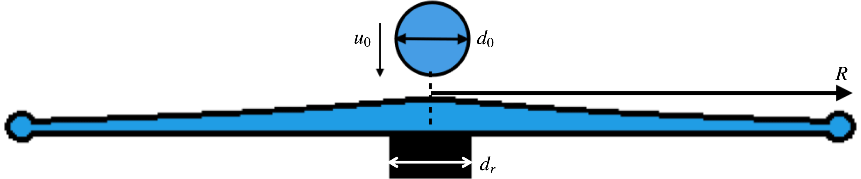
Here, we focus on a canonical unsteady fragmentation process occurring upon drop impact on a small target of comparable size to that of the impacting drop (figure 1). This fundamental framework enables us to gain insights into the selection of ubiquitous polydispersed droplet size and speed distributions from unsteady fragmentation, which can be generalized and translated to a wide range of applications. We conducted systematic experiments and developed droplet and ligament detection, tracking and connection algorithms that capture all ejected droplets during rim fragmentation and link them to their ligaments of origin. The experiments and algorithms are described in § 2. These algorithms allowed us to discover three ejection modes of droplets during unsteady sheet fragmentation, which are discussed in § 3. We discuss the size distribution of ejected droplets in § 4 and show that their cumulative size distribution over time is shaped by the time evolution of their instantaneous population mean size, which we also show to be fully determined by their ligament of origin. The analogous discussion of the cumulative versus instantaneous droplet speed distributions is in § 5.
Schematic diagram of drop impact on a small surface of comparable size to that of the impacting drop, transformed into a horizontal expanding sheet. The optimal rod-to-drop diameter ratio used in the experiments is
 $\unicode[STIX]{x1D702}=d_{r}/d_{0}=1.44$
(Wang & Bourouiba Reference Wang and Bourouiba2017).

2 Observations and droplet–ligament connection algorithm
Experimental conditions used from impacting drop diameter
 $d_{0}$
, impacting velocity
 $u_{0}$
, to associated
 $We=\unicode[STIX]{x1D70C}u_{0}^{2}d_{0}/\unicode[STIX]{x1D70E}$
and
 $Re=u_{0}d_{0}/\unicode[STIX]{x1D708}$
, where
 $\unicode[STIX]{x1D70C}=1.0\times 10^{3}~\text{kg}~\text{m}^{-3}$
,
 $\unicode[STIX]{x1D708}=1.0\times 10^{-6}~\text{m}^{2}~\text{s}^{-1}$
and
 $\unicode[STIX]{x1D70E}=72~\text{mN}~\text{m}^{-1}$
, are the density, kinematic viscosity and surface tension of the impacting drop, respectively.
 $N_{exp}$
is the number of experiments carried for each Weber number and
 $N_{drop}$
the average number of secondary droplets ejected for each experiment.

We conducted systematic experiments of canonical unsteady sheet fragmentation by impacting a drop on a cylindrical rod of comparable size to that of the drop. An impacting drop of diameter
 $d_{0}=4.33\pm 0.05$
mm is released by a needle from three different heights. Drops are made of water and nigrosin dye at concentration
 $1.2~\text{g}~\text{l}^{-1}$
, with density
 $\unicode[STIX]{x1D70C}=1.0\times 10^{3}~\text{kg}~\text{m}^{-3}$
, surface tension
 $\unicode[STIX]{x1D70E}=72~\text{mN}~\text{m}^{-1}$
and kinematic viscosity
 $\unicode[STIX]{x1D708}=1.0\times 10^{-6}~\text{m}^{2}~\text{s}^{-1}$
. The rod is made of stainless steel with smooth top surface with contact angle between
 $52^{\circ }$
and
 $81^{\circ }$
. The diameter of the rod is 6.25 mm with a rod-to-drop size ratio of 1.44, which allows for a horizontal sheet expansion and negligible surface viscous dissipation (Wang & Bourouiba Reference Wang and Bourouiba2017). We use high-speed cameras to record the entire fragmentation process from both top and side views simultaneously. A monochrome high-speed camera is used to record the impacts from the top at 20 000 frame per second (fps) and with
 $768\times 768$
pixel resolution. A colour camera is positioned on the side to record at 5000 fps and with
 $1280\times 1000$
pixel resolution. The impact velocity of the drops for each experiment is directly measured from the side camera. The detailed experimental conditions and their associated Weber number,
 $We=\unicode[STIX]{x1D70C}u_{0}^{2}d_{0}/\unicode[STIX]{x1D70E}$
, and Reynolds number,
 $Re=u_{0}d_{0}/\unicode[STIX]{x1D708}$
, are summarized in table 1.
Conventionally (Fantini, Tognotti & Tonazzini Reference Fantini, Tognotti and Tonazzini1990; Yarin & Weiss Reference Yarin and Weiss1995; Villermaux & Bossa Reference Villermaux and Bossa2011; Thoroddsen et al. Reference Thoroddsen, Takehara and Etoh2012; Peters, van der Meer & Gordillo Reference Peters, van der Meer and Gordillo2013), drop size distributions were obtained by measuring the diameter of all the droplets seen in a single image at the end of a fragmentation event or using a sequence of images with fixed temporal intervals spanning the duration of the fragmentation. On each image, droplet contours are detected and their diameter is inferred from the detected enclosed area. Such approaches are accurate for either droplets ejected continuously in steady fragmentation, such as a stationary Savart sheet (Savart Reference Savart1833a ,Reference Savart b ; Clanet & Villermaux Reference Clanet and Villermaux2002), or for droplets ejected simultaneously, such as at the final breakup stage of an expanding sheet upon drop impact on a rod (Villermaux & Bossa Reference Villermaux and Bossa2011). For continuous droplet ejection throughout unsteady sheet fragmentation, a single image cannot capture the size and speed of all droplets ejected. When using sequences of frames (Yarin & Weiss Reference Yarin and Weiss1995), if the time difference between two consecutive frames is too large, rapidly moving drops are missed. If the time difference is too small, double counting of slow droplets occurs. Both artefacts can lead to distortion of the final droplet size distribution produced. Moreover, the ejection time of each droplet, critical to quantifying unsteady fragmentation, is also missed by such approaches.
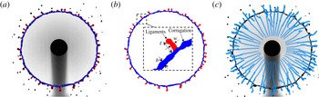
To guarantee accuracy in the capture of each ejected droplet without missing or double-counting sub-samples, we developed a ligament–droplet connection algorithm linking each ejected droplet to the ligament from which it detaches. The algorithm first captures the outline of each ligament at each time, and tracks its shape and location over time. Figure 2(a) illustrates the capture of both inner and outer contours of the rim–ligament system by our algorithm. We track local protrusions considered as ligaments when their length
 $\ell$
becomes larger than the local, instantaneous rim thickness
 $b$
(figure 2
b). The tracks in figure 2(c) show the trajectories of ligament tips throughout the sheet expansion. Droplets are continuously shed via ligament breakup. When a new droplet is shed, its ligament of origin suddenly shrinks. Thus, at each time, we consider new ejected droplets as those in the vicinity of a ligament that suddenly shrank. Based on this principle, our algorithm captures all droplets and identifies their ligament of origin, and precise detachment time.
(a) Sheet fragmentation and (b) separation of the rim and ligament based on the inner and outer contours of the sheet detected by our algorithm. The inset shows a local rim–ligament structure, defining the ligament length
 $l$
, its width
 $w$
and rim thickness
 $b$
. (c) Trajectories of the tip of all ligaments growing from the rim during the entire sheet expansion.

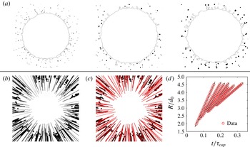
(a) Droplets detected by image processing at times
 $t=0.2\unicode[STIX]{x1D70F}_{cap}$
,
 $t=0.4\unicode[STIX]{x1D70F}_{cap}$
and
 $t=0.6\unicode[STIX]{x1D70F}_{cap}$
. The black line shows the outer contour of the rim and ligament. (b) Superposition of the trajectory of the droplets detected. (c) Tracks followed by each droplet. Solid lines indicate droplet trajectories captured by the algorithm. (d) Time evolution of the radial position of droplets with respect to the impact point, showing that the droplets move at constant speed.

Upon its ejection from a ligament, we can determine the size, speed and trajectory of a droplet. We developed a droplet-tracking algorithm specifically tailored to handle a wide range of droplet sizes and speeds. The algorithm first captures the contour of ejected droplets at each time (figure 3 a) and then tracks their position over time accounting for the unsteadiness of the problem. By superposing the contour of droplets from different frames on a single image, we can rebuild the trajectories of all ejected droplets experimentally (figure 3 b), matching very well with the tracking results of our algorithm (figure 3 c).
As described above, the traditional approach to measuring the size of ejected droplets is to first detect their contour and then calculate their diameter from the enclosed area within the detected contour. Two factors affect the accuracy of drop size measurements. First, the contour on an image is detected from the gradient of the local intensity on the image. The pixels with highest local gradient around the object are considered part of its contour. Such a method has higher accuracy when the contrast between the object and the background is high and the object is well in focus, which we ensured. The error of measurement of our droplet sizes is of the order of a pixel size, with images of approximately
 $40~\unicode[STIX]{x03BC}\text{m}~\text{pixel}^{-1}$
. The droplets ejected during fragmentation, except for the satellite droplets described in § 3, are larger than 0.4 mm with a measurement error smaller than 10 %. Second, the traditional approach used to compute droplet diameters based on the area
 $A_{d}$
enclosed within the detected contour:
 $d_{A}=\sqrt{4A_{d}/\unicode[STIX]{x03C0}}$
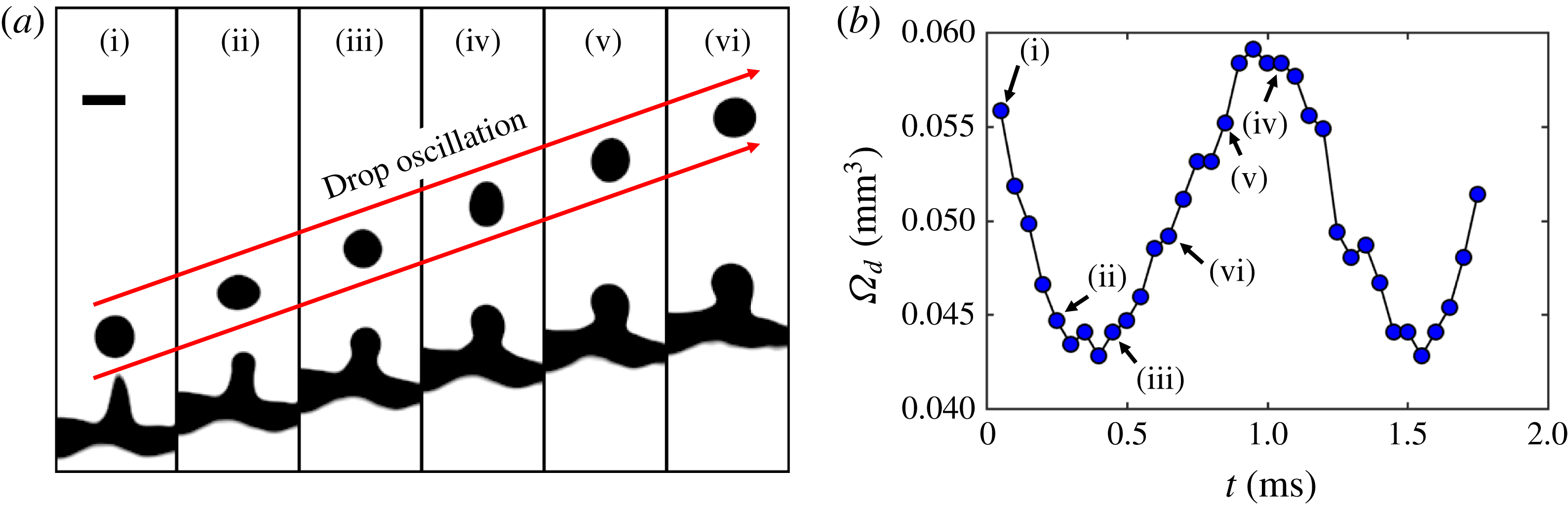
is accurate when the droplet is spherical. Yet, the ejected droplets oscillate along their trajectories, under the balance of the inertia and surface tension (figure 4
a). Figure 4(b) shows the time evolution of the droplet volume
 $\unicode[STIX]{x1D6FA}_{d}$
calculated from the area-based diameter with
 $\unicode[STIX]{x1D6FA}_{d}=\unicode[STIX]{x03C0}d_{A}^{3}/6$
, clearly showing that such volume oscillates spontaneously, violating mass conservation. Since the evaporation time scale of droplets of
 $O(0.1~\text{mm})$
diameter is much larger than the fragmentation time scale, the volume of the droplet should remain constant within our duration of observation. The relative difference between the diameter of an oscillating droplet calculated from its area can reach up to 10 %, the same order of magnitude as that of a pixel-size error. The more accurate method of calculation of droplet diameter should be based on a volume estimation, that is constant over time, rather than area which changes with time. The two approaches are equivalent when the drop is exactly spherical. Our tracking algorithm detect the shape of each droplet and extract the times at which eccentricity is closest to 0 (spherical). The diameter is extracted from these selected times.
(a) Sequence of oscillation of a droplet after its detachment from its ligament of origin. The time interval between images is 0.2 ms and the scale bar is 0.5 mm. (b) Time evolution of the droplet volume
 $\unicode[STIX]{x1D6FA}_{d}$
calculated from an area-based diameter
 $d_{A}=\sqrt{4A_{d}/\unicode[STIX]{x03C0}}$
, where
 $A_{d}$
is the area of the droplet shown in (a).
 $t=0$
refers to the time at which the droplet detaches from the ligament. The data corresponding to the times shown in (a) are labelled in (b).

The speed of the droplets is obtained from calculation of the difference between the position of two consecutive frames. Two aspects affect the accuracy of such speed measurement. First, if a drop moves too fast, the droplet appears as a long blurred trajectory with low contrast. In order to capture such fast moving droplets, while not sacrificing image resolution, we reduce the shutter speed to
 $5~\unicode[STIX]{x03BC}\text{s}$
, 10 times higher than the frame rate, which enables us to capture droplets with velocities smaller than
 $10~\text{m}~\text{s}^{-1}$
. The speed of the droplets ejected during unsteady sheet fragmentation are within this range. In fact, we do see tiny droplets ejected at the very early stage of sheet expansion of the order of 1 pixel size or less and leaving a blurred trajectory in the image, with very low contrast. The droplets on which our study focus are shed via a hydrodynamic instability of the expanding sheet in the air, while such very tiny droplets are ejected even when the sheet edge is still on the rod/solid surface, making the physics involved distinct, as no-slip, air trapping and precursor film ejections are involved. Our study does not focus on these tiny droplet closer to the micro-splashed droplets discussed in Thoroddsen et al. (Reference Thoroddsen, Takehara and Etoh2012) and Riboux & Gordillo (Reference Riboux and Gordillo2015). The second aspect is the effect of pixelization. The accuracy for the droplet speed measurement from calculation of the difference between the droplet positions in two consecutive frames is 1 pixel/frame, corresponding to
 $0.8~\text{m}~\text{s}^{-1}$
here, which could lead to large errors when the speed of droplets is less than that accuracy limit. To reduce the effect of pixelization, our algorithm can detect the time when the speed of droplets is smaller than that limit, and then re-calculates the speed by averaging the speed among multiple consecutive frames around that time. The smaller the droplet speed is, the more consecutive frames are needed to reduce the speed measurement error. The relative error for the speed measurement is reduced to up to 20 %.
Figure 3(d) shows the time evolution of the radial position of the ejected droplets with respect to the impact point, showing that droplets travel at a constant speed during our interval of observation. Since we are able to track the tip of a ligament as mentioned above, the same approach is used to measure the tip speed of ligaments. We discuss the relation between the speeds of droplets and ligament tips in § 5.
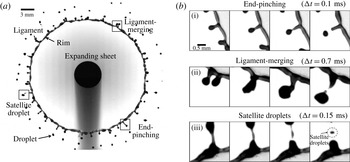
(a) Sheet fragmentation upon drop impact on a rod of comparable size to the impacting drop. The expanding sheet is bounded by a rim on which ligaments grow to finally eject secondary droplets. (b) Sequence of events for three different types of secondary droplet ejections: end-pinching, ligament-merging and satellite droplets.

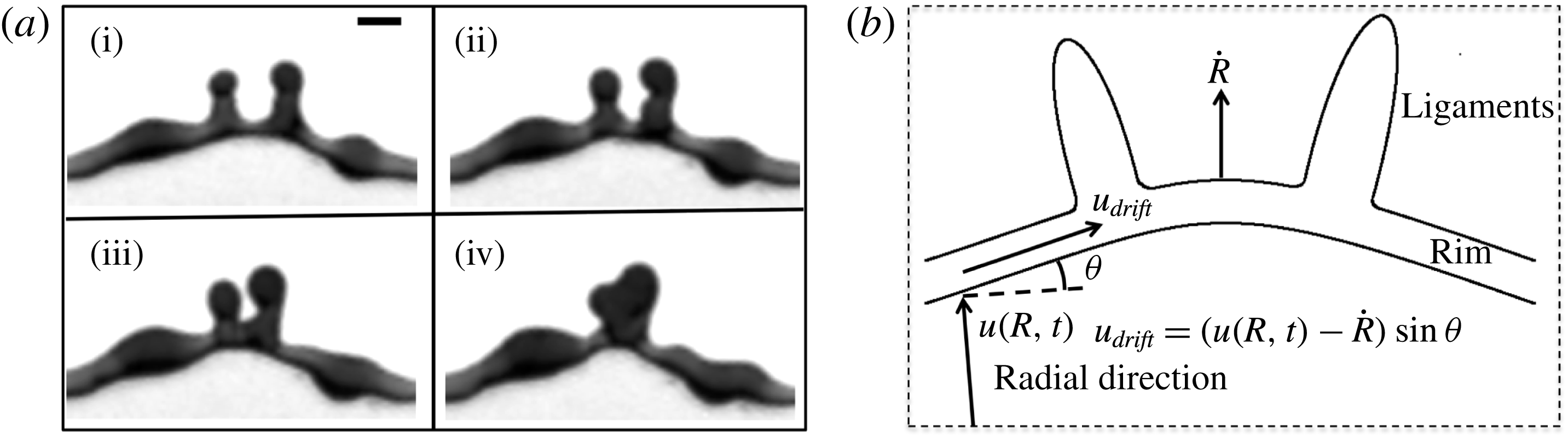
(a) Sequence showing the shift of ligaments induced by local cusps, leading to the collision and merger of two ligaments. Time difference between images is 0.25 ms. Scale bar is 1 mm. (b) Schematic diagram of drifting ligaments.

3 Three modes of droplet ejection
Drop shedding occurs continuously during sheet expansion in the form of three modes of droplet ejection (figure 5 b). The first mode is end-pinching (figure 5 b-i). Capillary deceleration of the tip of the ligament combined with fluid entering through the ligament foot leads to bulge formation at the tip. A neck forms between the bulged tip and the rest of the ligament and narrows progressively until a droplet is ejected. This mode was reported in prior studies of jets as end-pinching (Schulkes Reference Schulkes1996; Gordillo & Gekle Reference Gordillo and Gekle2010; Hoepffner & Paré Reference Hoepffner and Paré2013).
The second mode of ejection is ligament-merging followed by end-pinching (figure 5
b-ii). Ligaments do not always stay at a fixed angular position on the rim, but shift along it. Due to a local wedge geometry formed by the rim (figure 6). Such wedge shape is similar to that around Savart sheets referred to as cusps (Gordillo, Lhuissier & Villermaux Reference Gordillo, Lhuissier and Villermaux2014). Cusps are caused by the non-uniform distribution of mass per unit arc-length. The fluid from the sheet entering the rim accumulates around corrugations and protrusions that can eventually become ligaments, at which point the increase in mass per unit arc-length reduces capillary deceleration locally, thus exacerbating local deformation (figure 6
a). Around the cusps, the rim is no longer perpendicular to the incoming sheet radial influx, but is at an angle
 $\unicode[STIX]{x1D703}$
from it (figure 6
b). Such angle induces a drift velocity along the rim. In the reference frame of the rim, the incoming velocity
 $u_{in}(t)=u(R(t),t)-{\dot{R}}(t)$
, where
 $R(t)$
is the radius of the sheet at time
 $t$
,
 ${\dot{R}}(t)$
is the radial velocity of the rim and
 $u(R(t),t)$
is the fluid velocity in the sheet at radius
 $R(t)$
. The drift velocity induced is the projection of the incoming velocity
 $u_{in}$
in the direction longitudinal to the rim:
 $$\begin{eqnarray}\displaystyle u_{drift}=u_{in}(t)\sin \unicode[STIX]{x1D703}\quad \text{with}~u_{in}(t)=u(R(t),t)-{\dot{R}}(t). & & \displaystyle\end{eqnarray}$$
The velocity profile of the expanding sheet upon drop impact on a rod inferred from prior studies (Rozhkov, Prunet-Foch & Vignes-Adler Reference Rozhkov, Prunet-Foch and Vignes-Adler2004; Villermaux & Bossa Reference Villermaux and Bossa2011) and measured by Wang & Bourouiba (Reference Wang and Bourouiba2017) is
 $u(r,t)=r/t$
. In figure 6(a), we measure
 $u_{drift}\approx 0.32~\text{m}~\text{s}^{-1}$
, and we estimate
 $u_{in}=R(t)/t-{\dot{R}}(t)\approx 2.58~\text{m}~\text{s}^{-1}$
. The angle measured is
 $\unicode[STIX]{x1D703}\approx 8\pm 2^{\circ }$
, giving a prediction of drift velocity
 $u_{drift}=2.58\times \sin (8)=0.36~\text{m}~\text{s}^{-1}$
in good agreement with our experimental measurement. The shifting ligaments collide and merge (figure 5
b-ii), resulting into a typically corrugated final ligament. Despite such corrugation, the resulting ligament continues to shed only one drop from its tip immediately upon merger. We refer to end-pinching and ligament-merging droplets as primary droplets.
The third mode of ejection creates satellite droplets (figure 5 b-iii). During necking between the bulged tip and the rest of its ligament, the neck elongates and thins. Upon breakup, the neck can form one or multiple small satellite droplets. Such satellite droplets are much smaller than primary droplets produced by the first two modes and they account for only l0 % of all droplets ejected during sheet expansion. Thus, the satellite droplets are not involved in the discussion of the droplet size and speed distributions in subsequent sections.
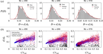
(a) Distributions of the diameter of primary droplets ejected during the entire fragmentation process for three different Weber numbers. Droplet diameters are non-dimensionalized by the diameter
 $d_{0}$
of the impacting drop. The distributions are all skewed and can be fitted by a gamma distribution of the order shown. (b) Temporal evolution of the diameter of ejected droplets for three different Weber numbers. Time is non-dimensionalized by the capillary time scale
 $\unicode[STIX]{x1D70F}_{cap}=\sqrt{\unicode[STIX]{x1D70C}\unicode[STIX]{x1D6FA}/\unicode[STIX]{x03C0}\unicode[STIX]{x1D70E}}$
. Each data point corresponds to one ejected droplet. Ejected droplets are separated into the three groups described in figure 5(b).

4 Distribution of droplet sizes
4.1 Cumulative size distribution of droplets
Our study focuses on the size distribution of droplets ejected by the first two modes defined as primary droplets in § 3. They account for 90 % of the total number of droplets ejected during unsteady sheet fragmentation. Figure 7(a) shows the distribution of the diameter of primary droplets ejected during the entire sheet expansion. The distributions are skewed for all three Weber numbers. When attempting to fit them with a gamma distribution proposed in Villermaux, Marmottant & Duplat (Reference Villermaux, Marmottant and Duplat2004)
 $$\begin{eqnarray}\displaystyle P(n,x=d/\langle d\rangle )=\frac{n^{n}}{\unicode[STIX]{x1D6E4}(n)}x^{n-1}\text{e}^{-nx}, & & \displaystyle\end{eqnarray}$$
the order
 $n$
changes severely with impact Weber number, departing from values given by Villermaux & Bossa (Reference Villermaux and Bossa2011). Note that the underlying physics of (4.1) is that droplets fragment from elongated corrugated ligaments, where the coalescence and aggregation process of corrugations selects the droplet size distribution. As discussed in § 3, here a ligament only sheds one droplet from its tip at a time in an end-pinching process. Thus, aggregation–coalescence of corrugations along ligaments do not apply to rationalize the drop size distribution of unsteady expanding sheets examined here.
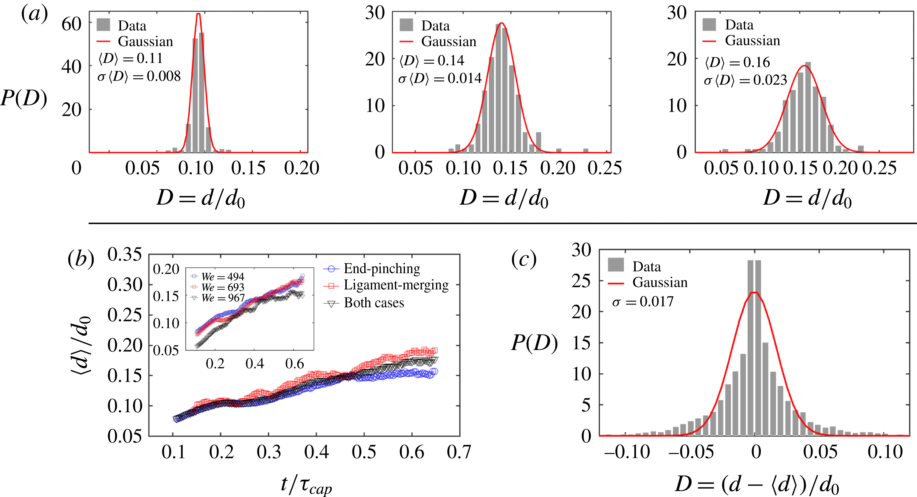
(a) Instantaneous distributions of the diameter of primary droplets at three different times
 $t=0.2\unicode[STIX]{x1D70F}_{cap}$
,
 $0.4\unicode[STIX]{x1D70F}_{cap}$
and
 $0.6\unicode[STIX]{x1D70F}_{cap}$
for
 $We=693$
, where
 $\unicode[STIX]{x1D70F}_{cap}=\sqrt{\unicode[STIX]{x1D70C}\unicode[STIX]{x1D6FA}/\unicode[STIX]{x03C0}\unicode[STIX]{x1D70E}}$
is the capillary time scale characterizing the sheet expansion and fragmentation process, and
 $t=0.4\unicode[STIX]{x1D70F}_{cap}$
is the time when the sheet reaches its maximum extension. The instantaneous distributions are symmetric and Gaussian. (b) Time evolution of the mean diameter of droplets from different ejection modes for
 $We=693$
. The inset shows the comparison of the mean diameters of primary droplets for three different
 $We$
. (c) The total distribution of the diameter of all primary ejected droplets for
 $We=693$
after adjustment for the instantaneous mean diameter is not skewed.

Figure 7(b) shows the measured diameters of ejected droplets with their detachment time. Time is non-dimensionalized by the capillary time scale
 $\unicode[STIX]{x1D70F}_{cap}=\sqrt{\unicode[STIX]{x1D70C}\unicode[STIX]{x1D6FA}/\unicode[STIX]{x03C0}\unicode[STIX]{x1D70E}}$
that characterizes the sheet expansion and fragmentation process, where
 $\unicode[STIX]{x1D6FA}$
is the volume of the impacting drop. Each data point corresponds to one ejected droplet. Ejected droplets are separated into the three ejection modes described in § 3. Except for the less than 10 % of all droplets that are shed as satellite droplets, the mean diameter of primary droplets clearly increases with time (figure 8
b). Thus, it is the superposition of distributions with shifting mean that leads to the skewed total distribution of droplet sizes (figure 3
a). To verify this, we calculate the instantaneous distribution of primary droplet diameters at each time by considering data around that time over a small time interval of 0.15 ms duration, within which the unsteadiness of the sheet fragmentation is negligible. Figure 8 shows that the instantaneous distribution at each time is symmetric and Gaussian. Figure 8(c) shows the total distribution of diameters of ejected droplets after subtraction of the instantaneous mean diameter shown in figure 8(b). The total distribution adjusted by its unsteady instantaneous mean diameter is symmetric. This verifies that the skewness of the total distribution shown in figure 7(a) is caused by the unsteady temporal evolution of instantaneous mean droplet diameters.
4.2 End-pinching ligament width shapes droplet diameter
Discovering that unsteadiness shapes the skewness of the total distribution of droplet diameters, we examine the time evolution of the population mean droplet diameter
 $\langle d\rangle$
. As discussed in § 3, droplets are mainly ejected from ligament tips. Our tracking algorithm (§ 2) allows us to link each ejected droplet to its original ligament. Figure 9(a) shows the ratio,
 $R=d/w$
, of the diameter
 $d$
of ejected droplet to the width
 $w$
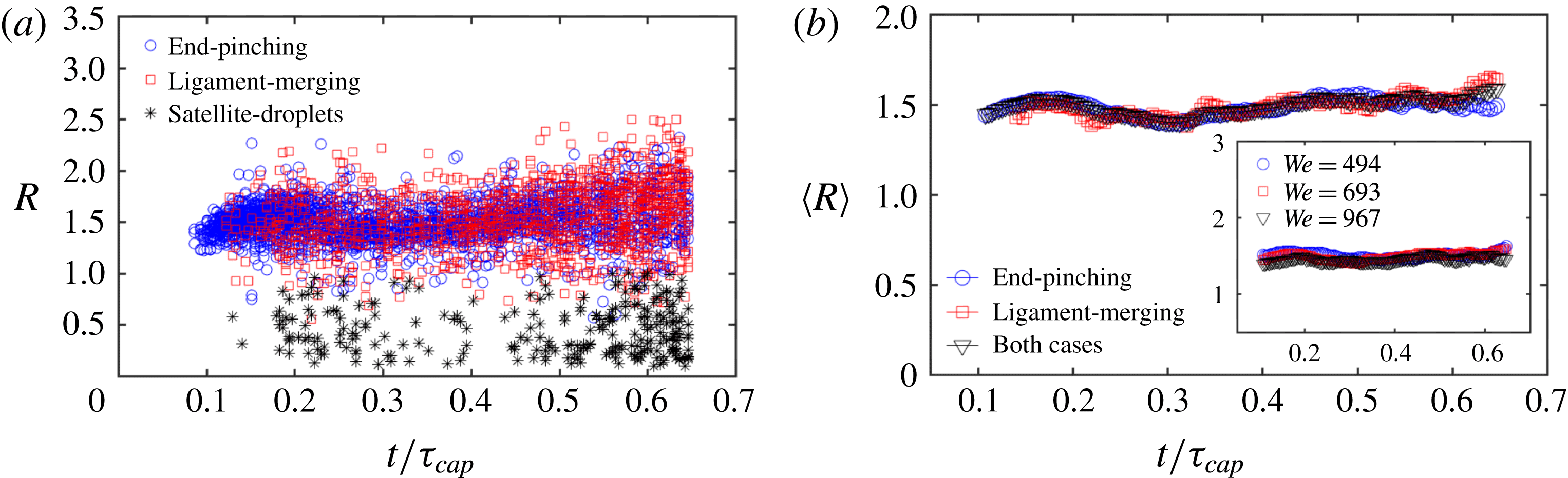
of its original ligament as a function of time. Except for satellite droplets again, less than 10 % of total droplets, the mean droplet–ligament size ratio for primary droplets is constant over time:
 $\langle R\rangle =\langle d/w\rangle \approx 1.5$
(figure 9
b), and is independent of impact Weber number (inset of figure 9
b). This shows that the diameter of droplets is determined deterministically by the width of the ligament shedding them, and that such droplet–ligament size ratio is local and universal, i.e. independent of impact
 $We$
and sheet expansion.
In the case of a long cylindrical liquid ligament, the Rayleigh–Plateau instability (Rayleigh Reference Rayleigh1878) typically triggers fragmentation with a fastest growing wavelength of
 $\unicode[STIX]{x1D706}=9w/2$
, where
 $w$
is the initial cylinder diameter. Based on mass conservation, the volume of the produced droplets at such wavelength would be
 $$\begin{eqnarray}\displaystyle \frac{\unicode[STIX]{x03C0}}{6}d^{3}=\frac{9}{2}w\left(\frac{1}{4}\unicode[STIX]{x03C0}w^{2}\right),\quad \text{thus}~\frac{d}{w}=1.89, & & \displaystyle\end{eqnarray}$$
which is larger than
 $\langle R\rangle =\langle d/w\rangle \approx 1.5$
. However, the Rayleigh–Plateau (R–P) instability strictly holds for infinite or semi-infinite liquid cylinders. As discussed in § 3, droplets ejected during sheet fragmentation are shed from the tip of finite ligaments that are too short for the R–P instability to apply. Instead, droplets are shed via end-pinching which is caused by the retraction of ligament tips. Schulkes (Reference Schulkes1996) studied end-pinching numerically for free liquid jets of arbitrary viscosity, finding that the evolution of the ligament tip depends on the Ohnesorge number
 $Oh=\unicode[STIX]{x1D708}\sqrt{\unicode[STIX]{x1D70C}/w\unicode[STIX]{x1D70E}}$
, a measure of competition between viscous forces, inertia and surface tension, similar to the retraction of the rim of a sheet (Savva & Bush Reference Savva and Bush2009). Ligaments of large Ohnesorge number
 $O(Oh)>O(1)$
are stable during retraction, while ligaments of small Ohnesorge number
 $O(Oh)<O(0.1)$
form a neck close to the ligament tip. When
 $Oh$
is much smaller
 $O(Oh)<O(0.001)$
, the ligament is unstable and the neck narrows quickly until end-pinching. The critical value of
 $Oh$
below which end-pinching occurs was found to be
 $Oh\approx 10^{-2}$
(Schulkes Reference Schulkes1996). Based on the width of ligaments shown in figure 11, the range of
 $Oh$
here is
 $5.3\times 10^{-4}<Oh<8.5\times 10^{-3}$
, for which end-pinching holds. A fully analytic solution describing end-pinching remains elusive since vortex shedding was observed to occur experimentally at ligament tips during necking (Hoepffner & Paré Reference Hoepffner and Paré2013), jeopardizing the validity of a one-dimensional approximation of the problem (Eggers & Dupont Reference Eggers and Dupont1994). Schulkes (Reference Schulkes1996) found numerically that the ratio of the diameter of a droplet ejected by end-pinching to the width of its ligament of origin is 1.5–1.6, which is close to our experimental data (figure 9).
(a) The ratio
 $R$
of the diameter
 $d$
of each secondary droplet with the width
 $w$
of its original ligament as a function of detaching time for
 $We=693$
. Droplets are separated into three scenarios as described in figure 5(b). (b) Time evolution of the mean droplet–ligament size ratio of ejected droplets of different scenarios for
 $We=693$
. The ratio
 $R$
of primary droplets remain constant over time. The inset shows that ratio
 $\langle R\rangle \approx 1.5$
holds for all
 $We$
.

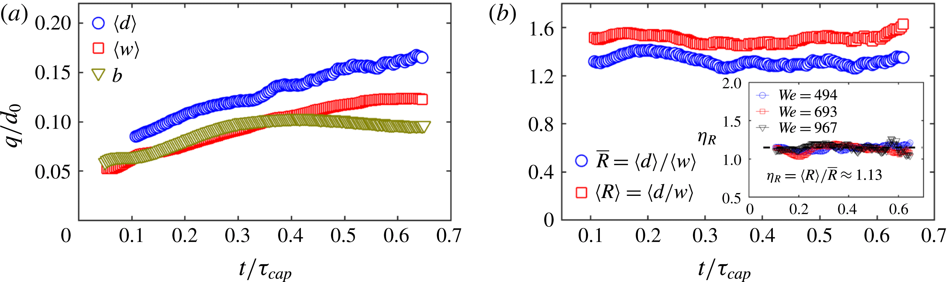
(a) Time evolution of the mean droplet diameter
 $\langle d\rangle$
, the mean ligament width
 $\langle w\rangle$
and the sheet rim thickness
 $b$
for
 $We=693$
. (b) The ratio
 $\bar{R}=\langle d\rangle /\langle w\rangle$
remains constant. However, compared with the mean size ratio of droplet–ligament pairs
 $\langle R\rangle =\langle d/w\rangle$
, a systematic gap between these two ratios persists. The inset shows the ratio of
 $\unicode[STIX]{x1D702}_{R}=\langle R\rangle /\bar{R}$
to be constant over time and independent of
 $We$
, with a value of 1.13.

Gordillo & Gekle (Reference Gordillo and Gekle2010) studied end-pinching at the tip of a Worthington jet, which is a stretched liquid jet. Stretching rate can affect the ligament-tip breakup. Scaling analysis compared with numerical simulation led Gordillo & Gekle (Reference Gordillo and Gekle2010) to quantify
 $R$
as
 $$\begin{eqnarray}\displaystyle R=\frac{d}{w}=\left\{\begin{array}{@{}ll@{}}0.95We_{s}^{-1/7}\quad & \text{for}~We_{s}>0.08\\ 1.55\quad & \text{for}~We_{s}<0.08\end{array}\right.\quad \text{with}~We_{s}=\frac{\unicode[STIX]{x1D70C}w^{3}}{8\unicode[STIX]{x1D70E}}s_{0}^{2}, & & \displaystyle\end{eqnarray}$$
where
 $s_{0}$
is the stretching rate of the ligament
 $s_{0}=\dot{u}_{liga}/u_{liga}$
, with
 $u_{liga}$
the velocity of fluid entering the base of the ligament. Equation (4.3) indicates that when
 $We_{s}>0.08$
, the ligament is dominated by stretching and the droplet–ligament size ratio
 $R$
is affected by said stretching. In our experiments, we estimate that for each ligament
 $We_{s}\approx 0.05$
, below the stretching regime of
 $We_{s}>0.08$
. Using (4.3), the droplet–ligament size ratio would then be
 $R=d/w=1.55$
, in good agreement with our experiments.
In sum, we showed that the droplet ejection from unsteady sheet expansion is caused by end-pinching, rather than the R–P instability or corrugation–coalescence process of individual ligaments. We also showed that the droplet–ligament size ratio of end-pinching obtained numerically in prior literature on jets applies and is robust herein for the ligaments bounding the unsteady rim.
After considering the drop–ligament size ratio for each droplet–ligament pair, we now turn to the relation between the population mean droplet diameter
 $\langle d\rangle$
and the population mean ligament width
 $\langle w\rangle$
(figure 10
a). It is clear that the mean droplet diameter
 $\langle d\rangle$
follows the same trend as the mean ligament width
 $\langle w\rangle$
, consistent with figure 9. Figure 10(b) shows
 $\bar{R}=\langle d\rangle /\langle w\rangle \approx 1.3$
to be constant over time, but systematically smaller than
 $\langle R\rangle =\langle d/w\rangle \approx 1.5$
. The difference between the two
 $\unicode[STIX]{x1D702}_{R}=\langle R\rangle /\bar{R}\approx 1.12$
is constant and independent of Weber number (figure 10
b-inset). To understand the gap
 $\unicode[STIX]{x1D702}_{R}$
, we examine the width of ligaments during droplet shedding in more detail.
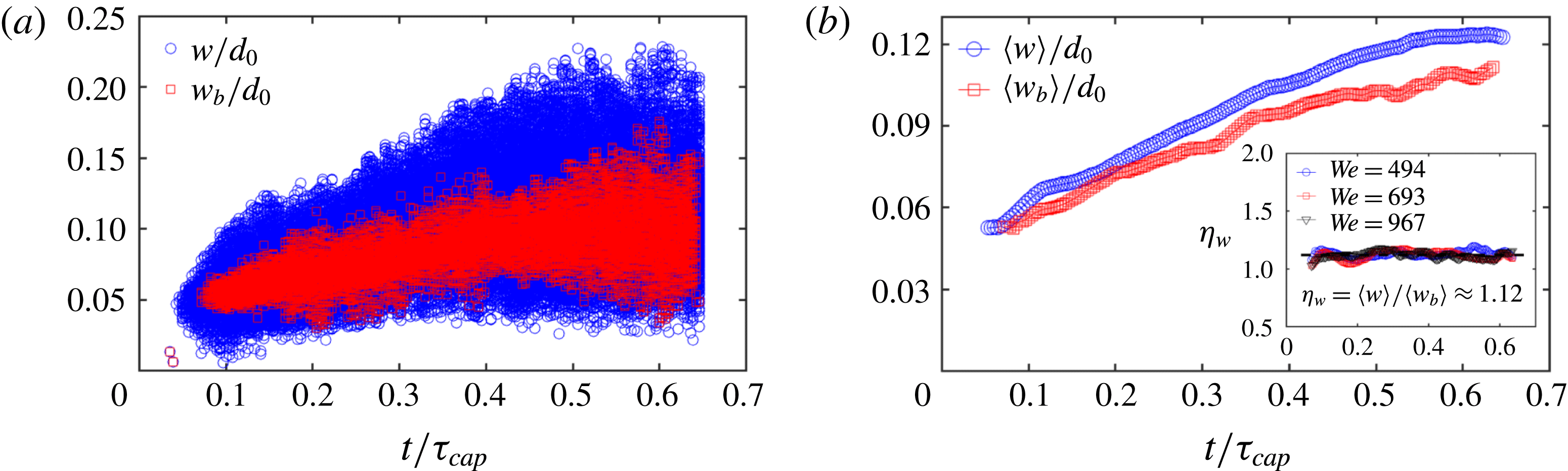
(a) Width of all ligaments (circle)
 $w$
and ligaments about to shed a droplet (square)
 $w_{b}$
as a function of time. (b) Time evolution of the corresponding mean widths
 $\langle w\rangle$
and
 $\langle w_{b}\rangle$
. The inset shows the ratio
 $\unicode[STIX]{x1D702}_{w}=\langle w\rangle /\langle w_{b}\rangle \approx 1.12$
to be constant and independent of
 $We$
.

Figure 11(a) shows the temporal evolution of the width
 $w$
of all ligaments detected compared to the width
 $w_{b}$
of those ligaments about to shed a drop, with their means shown in figure 11(b). The systematic gap between the two means
 $\unicode[STIX]{x1D702}_{w}=\langle w\rangle /\langle w_{b}\rangle \approx 1.12$
is also constant and independent of Weber number (figure 11
b-inset), and equal to the ratio
 $\unicode[STIX]{x1D702}_{R}=\bar{R}/\langle R\rangle$
. Thus, the difference between the mean droplet–ligament size ratio of each droplet–ligament pair
 $\langle R\rangle =\langle d/w\rangle$
and the ratio of the population mean droplet diameter with the population mean ligament width
 $\bar{R}=\langle d\rangle /\langle w\rangle$
is caused by the systematic difference in width between shedding
 $\langle w_{b}\rangle$
and non-shedding ligaments
 $\langle w\rangle$
. Ligaments about to shed a drop generally have time to extend into a slender shape, while non-shedding ligaments are typically close to bulged corrugations that are wider. Clarifying the origin of the particular value 1.12 of
 $\langle w\rangle /\langle w_{b}\rangle$
for end-pinching ligaments is of interest, but is beyond the scope of the present study.
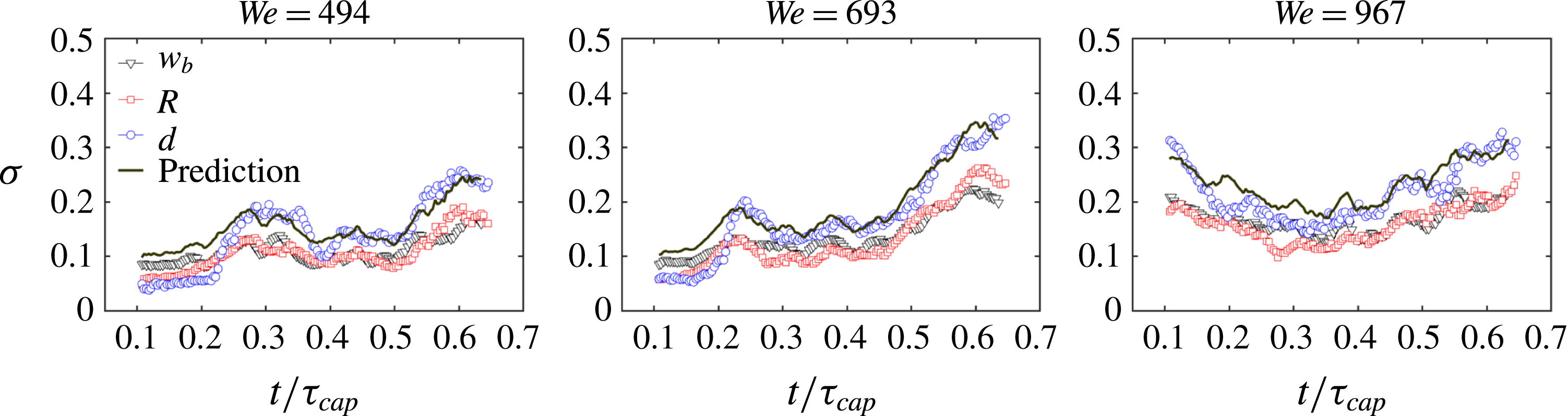
Comparison of time evolution of the standard deviation of the width of shedding ligaments
 $w_{b}$
, droplet–ligament size ratio
 $R$
and droplet diameter
 $d$
. The prediction of
 $\unicode[STIX]{x1D70E}(d)$
based on (5.3) is in very good agreement with the measurement.

Figure 9 shows the standard deviation of the width
 $w_{b}$
of ligaments that eject droplets, the size ratio of droplet–ligament pairs
 $R$
and the diameter of droplets
 $d$
as a function of time. Considering the mean
 $\langle R\rangle$
and
 $\langle w_{b}\rangle$
and standard deviation
 $\unicode[STIX]{x1D70E}(R)$
and
 $\unicode[STIX]{x1D70E}(w_{b})$
and, using
 $d=Rw_{b}$
, the standard deviation of the droplet diameter
 $\unicode[STIX]{x1D70E}(d)$
is
 $$\begin{eqnarray}\displaystyle \unicode[STIX]{x1D70E}^{2}(d)=(\unicode[STIX]{x1D70E}^{2}(R)+\langle R\rangle ^{2})(\unicode[STIX]{x1D70E}^{2}(w_{b})+\langle w_{b}\rangle ^{2})-\langle R\rangle ^{2}\langle w_{b}\rangle ^{2}. & & \displaystyle\end{eqnarray}$$
The prediction of standard deviation of ejected droplet diameter by (4.4) is in a good agreement with our experimental data (figure 12), confirming the robustness and accuracy of our measurements. Equation (4.4) combined with figure 10(b) show that the standard deviation of instantaneous droplet diameter around their mean size is directly inherited from the standard deviation of the width of their ligament of origin at breakup, and not from the breakup process itself.
5 Distribution of droplet ejection speed
5.1 Cumulative speed distribution of droplets
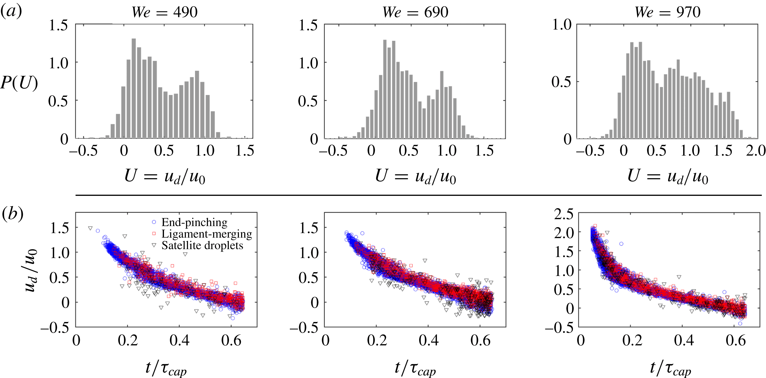
(a) Total distribution of speed of droplets ejected during the entire fragmentation process for three different Weber numbers (a Weber per column). The droplet speed distribution is non-dimensionalized by the impact speed
 $u_{0}$
of the falling drop. (b) Ejection speed of droplets as a function of time for three different Weber numbers with each data point corresponding to one ejected droplet. Ejected droplets are separated into the three different modes of ejections revealed in § 3.

Figure 13(a) shows the total speed distribution of droplets ejected throughout the unsteady sheet fragmentation for three different Weber numbers, non-dimensionalized by impact velocity
 $u_{0}$
. The total distribution of droplet speeds has a peculiar shape with two peaks. Figure 13(b) shows the measured speed of all ejected droplets, as a function of their detaching time, for three
 $We$
. As previously done, time is non-dimensionalized by the capillary time scale
 $\unicode[STIX]{x1D70F}_{cap}=\sqrt{\unicode[STIX]{x1D70C}\unicode[STIX]{x1D6FA}/\unicode[STIX]{x03C0}\unicode[STIX]{x1D70E}}$
, which is characteristic of the sheet expansion and fragmentation. Ejected droplets are separated in the three modes of ejection: end-pinching, ligament-merging and satellite droplet ejection identified in § 3. The ejection speed of droplets varies with time (figure 13
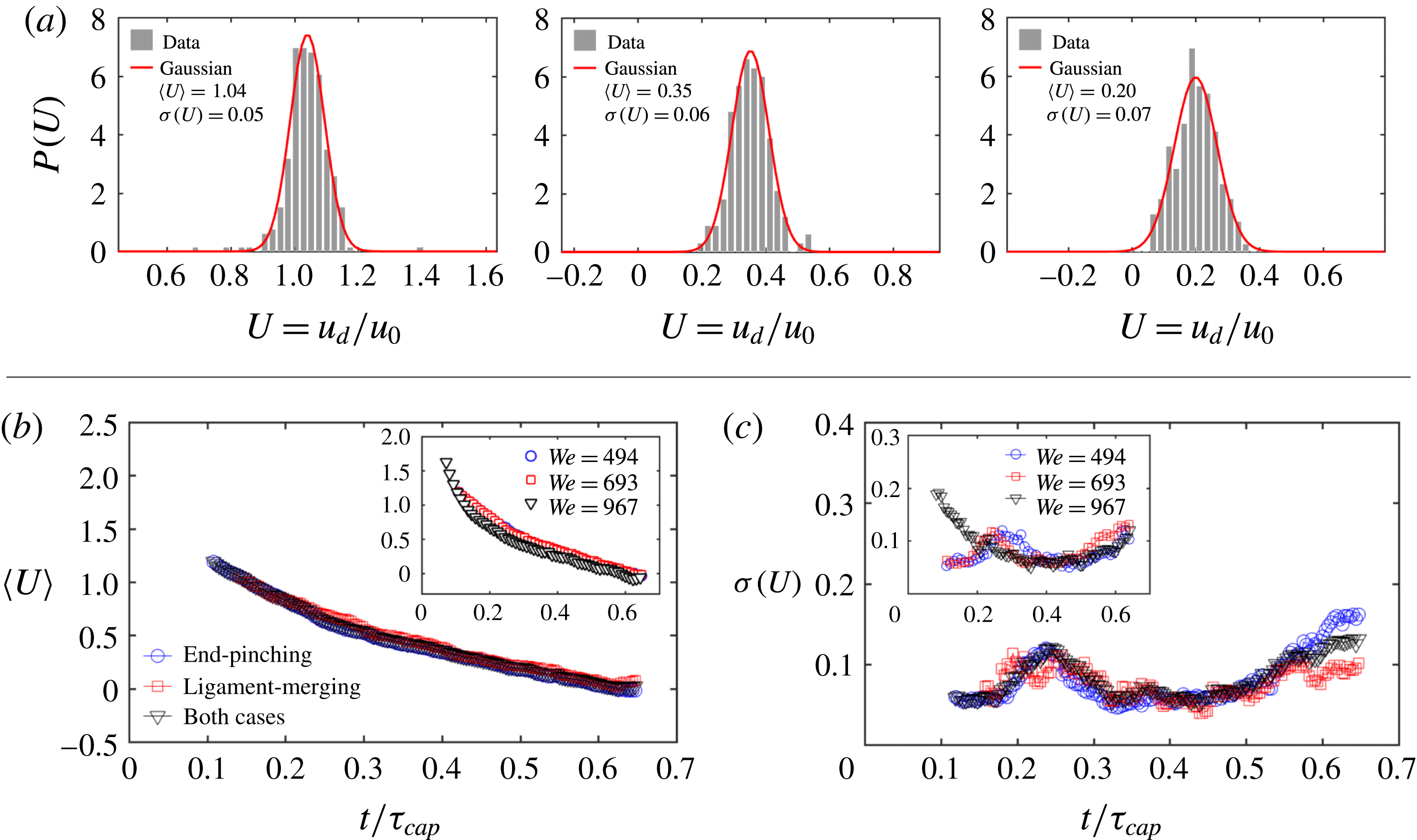
a) and is monotonically decreasing with time. Clearly, the total speed distribution is entirely shaped by the unsteadiness of the instantaneous mean of the ejection droplet speed. To verify this claim, we calculate the distribution of droplet ejection speed at each time as shown in figure 14(a). The instantaneous distribution is symmetric and Gaussian. Figure 14(b) shows the time evolution of the standard deviation of the ejection speed of droplets for different modes of ejection. Both the mean value and standard deviation of the ejection speed of end-pinching and ligament-merging droplets collapse onto a single curve, showing that the ejection speed is independent of the mode of ejection (figure 14
b,c).
(a) Instantaneous distribution of droplet speed at three different times
 $t=0.2\unicode[STIX]{x1D70F}_{cap}$
,
 $0.4\unicode[STIX]{x1D70F}_{cap}$
and
 $0.6\unicode[STIX]{x1D70F}_{cap}$
for
 $We=693$
, where
 $\unicode[STIX]{x1D70F}_{cap}=\sqrt{\unicode[STIX]{x1D70C}\unicode[STIX]{x1D6FA}/\unicode[STIX]{x03C0}\unicode[STIX]{x1D70E}}$
is the capillary time scale characterizing the sheet expansion.
 $t=0.4\unicode[STIX]{x1D70F}_{cap}$
is the time of maximum sheet radius. Instantaneous speed distributions are Gaussian with standard deviation given in the legend. (b) Mean ejection speed and (c) associated speed standard deviation of the droplets follow the same temporal trend for both end-pinching and ligament-merging modes of ejection.

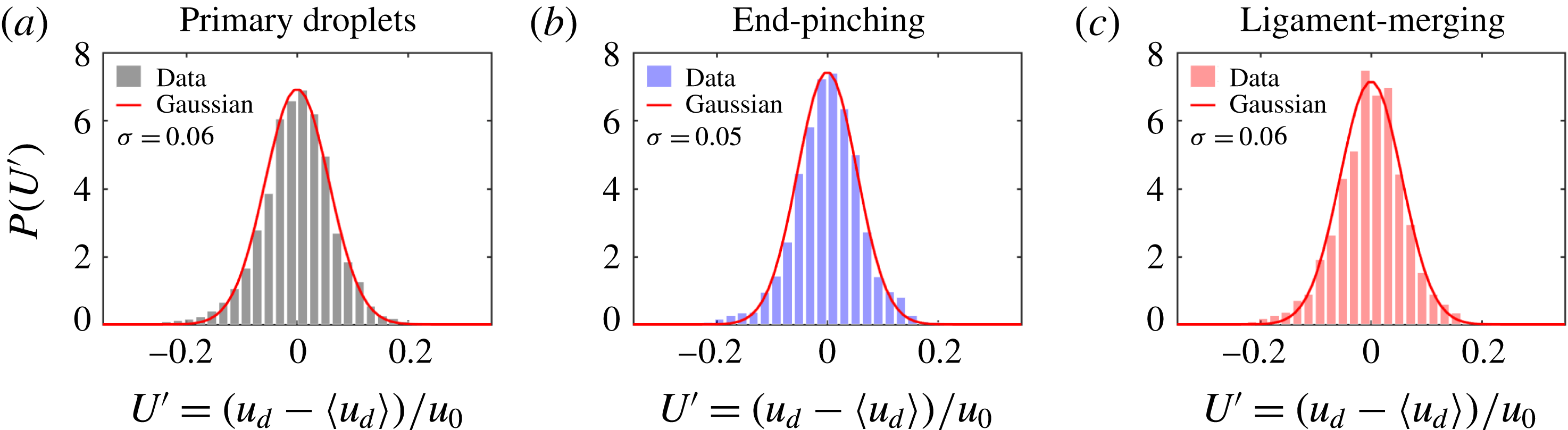
(a) The total distribution of ejection speeds of all droplets for
 $We=693$
after adjustment for instantaneous mean speed is Gaussian in contrast with the total speed distribution in figure 13. Clearly, unsteadiness of the instantaneous mean droplet speed shapes the skewness observed in figure 13. The same applies for the speed of (b) end-pinching and (c) ligament-merging droplets when considered separately.

Figure 15 shows the total distribution of the ejection speed of droplets after subtraction of the instantaneous mean speed (figure 14 b). The total adjusted distribution is symmetric and Gaussian. Thus, the peculiar shape of droplet speed distribution in figure 13 is due to the unsteadiness of the mean of ejection speed characterized by two regimes: an early time and late time speed evolution. Figure 15(b,c) shows that the total speed distribution of both end-pinching and ligament-merging droplets around their respective mean speeds are also Gaussian, confirming that the instantaneous ejection speed of droplets is independent of ejection mode.
5.2 Ligament speed shapes droplet speed
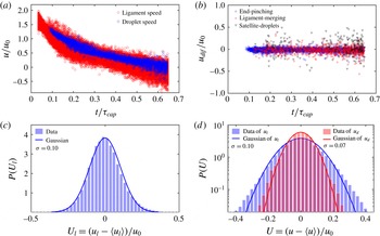
It is important to understand what determines the time evolution of mean droplet ejection speeds. Figure 16(a) shows that ligament-tip speed and droplet ejection speed fully overlap. This indicates that the drop ejection speed is determined by the speed of the tip of its ligament. Keller (Reference Keller1983) studied the retraction speed of the tip of free liquid jets and derived, by momentum conservation, that the tip retraction speed is constant
 $\sqrt{2\unicode[STIX]{x1D70E}/r_{l}}$
for uniform liquid jets of radius
 $r_{l}$
, which is similar to a Taylor–Culick speed for ruptured sheet retraction (Culick Reference Culick1960). Hoepffner & Paré (Reference Hoepffner and Paré2013) showed that the retraction tip speed of free liquid jets should be
 $\sqrt{\unicode[STIX]{x1D70E}/r_{l}}$
, which was verified by their own experimental data. The expression of Keller (Reference Keller1983) overestimates the speed by a factor of
 $\sqrt{2}$
due to their neglect of the inner curvature pressure of the cylindrical liquid jet, which was recovered in their derivation for the speed of the jet tip in Ting & Keller (Reference Ting and Keller1990). However, as shown in figure 16, the tip speed of a ligament growing out of a rim here is not constant. Instead, it follows the speed of the sheet rim. Indeed, the incoming fluid from the rim into the base of the ligament is determined by both the sheet expansion and rim destabilization. Based on our ligament-tracking algorithm introduced in § 2, we can link each droplet to the ligament from which it detaches. Figure 16(b) shows no distinction between the speed of a droplet and that of the ligament from which it detaches. That is, the ejection speed of each droplet is equal to the speed of its ligament’s tip prior to breakup.
(a) Temporal evolution of ejection speed of droplets and tip speed of ligaments. The overlap between the two shows that the speed of a ligament tip is inherited by the droplet right after detachment. (b) Zero velocity difference between the ejection speed of droplets and the tip speed of their ligaments of origin. (c) The total distribution of ligament-tip speeds adjusted for the moving instantaneous mean is symmetric and Gaussian. (d) Comparison of the distribution of ligament-tip speeds adjusted for the moving mean, as shown in (c), with that of the ejection speed of primary droplets, as shown in figure 15(a), on a semi-log plot, both being Gaussian. The width of the distribution of ligament-tip speeds is larger than that of primary droplet speeds.

Although the droplet speed is equal to the ligament-tip speed prior to detachment for each droplet–ligament pair, a systematic gap between the population mean ejection speed of droplets and the population mean speed of ligament tips exists (figure 18 a). To understand the origin of such gap, we need to examine the detachment more precisely.
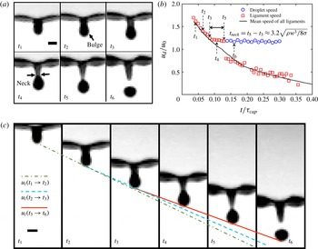
(a) Sequence of events leading to bulge formation and necking of the tip of the ligament prior to droplet detachment in the reference frame of the rim.
 $t_{3}$
is the time of start of necking, and
 $t_{5}$
is the time of droplet ejection. The time interval between images is 0.15 ms and the scale bar is 0.3 mm. (b) Time evolution of the tip speed of one ligament and the ejection speed of the secondary droplet detaching from it. The solid line gives the time evolution of the population mean speed of all ligament tips. (c) Sequence of ligament deformation prior to droplet detachment in the absolute reference frame.
 $t_{1}$
to
 $t_{6}$
correspond to the times shown in (a). The solid line shows that after necking, the ligament tip moves at constant speed, which is the same as the ejection speed of droplets after detachment. The dot-dash line connects the tip positions at
 $t_{1}$
and
 $t_{2}$
and the dash line connects the tip positions at
 $t_{2}$
and
 $t_{3}$
. By comparing the slopes of the three lines, it is clear that the ligament tip decelerates before necking at
 $t_{3}$
, which is consistent with (b). Scale bar is 0.3 mm.

Figure 17(a) shows the ligament deformation preceding droplet detachment in the form of a sequence. All images are given in the reference frame of the ligament. As described in § 4, capillary forces decelerate the tip of the ligament, while fluid continues to feed its foot, thus leading to fluid accumulation forming a bulged tip. A neck forms between the tip and the rest of the ligament. The neck width narrows progressively to finally break and eject a droplet. In figure 17(a), the ligament continues to grow on the rim at time
 $t_{1}$
. When time
 $t_{2}$
is reached, the ligament tip deforms into a bulge. At time
 $t_{3}$
, the bulged tip of the ligament is fully formed and the neck between the bulged tip and the ligament starts to form. Compared to the ligament at time
 $t_{4}$
where a clear neck is observed, the ligament maintains an approximate constant width between the bulged tip and the rim at time
 $t_{3}$
. Thus we consider
 $t_{3}$
as the onset of neck formation. At time
 $t_{5}$
, the width of the neck narrows down to 0, the ligament is close to pinching and ejection of the droplet. At time
 $t_{6}$
, the droplet is ejected by the ligament and moves freely in the air. Figure 17(b) shows the time evolution of the speed of one ligament’s tip (figure 17
a), compared to the population mean speed of ligament tips. From neck formation until final breakup, the speed of the ligament tip deviates from the population mean tip speed but remains constant, and equal to the final droplet ejection speed. This is readily observed when we look at the motion of ligaments in the absolute reference frame. Figure 17(c) shows the solid straight line which crosses the tip of the ligament from
 $t_{3}$
to
 $t_{5}$
, indicating that the tip speed remains constant throughout the duration of necking. The solid line also crosses the lower end of the ejected droplet at time
 $t_{6}$
. This shows that the constant speed of the ligament tip during necking is equal to the speed of the ejected droplet, which is consistent with figure 17(b). We can also see that the slope of the solid line is smaller than that of the dash line connecting the tip positions at
 $t_{2}$
and
 $t_{3}$
and the dot-dash line connecting the tip position at
 $t_{1}$
and
 $t_{2}$
, showing that the tip is decelerating before necking
 $t_{3}$
. Indeed, when the neck narrows, the capillary force exerted by the neck on the ligament tip,
 $F\approx \unicode[STIX]{x1D70E}\unicode[STIX]{x03C0}w_{n}$
, decreases, where
 $w_{n}$
is the width of the neck. Hence, the decrease of the capillary-induced deceleration of the tip.
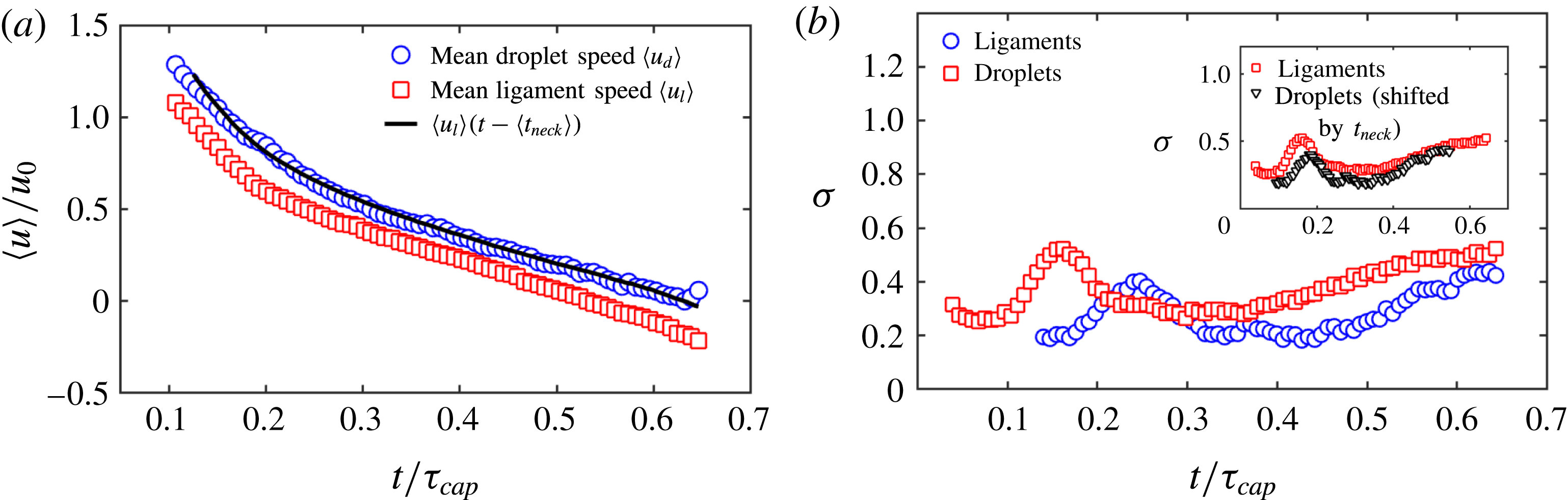
(a) Normalized time evolution of the population mean speed of secondary droplets (blue circle) compared with the population mean speed of ligament tip (red square) for
 $We=693$
. The velocity gap between the two is due to ligament necking. The mean speed of ligaments one necking time
 $t_{neck}$
(5.2) earlier (dash line) matches very well with the mean speed of droplets. (b) The standard deviation of the speed of secondary droplets follows the trend of ligament-tip speed, but also with a time delay of
 $t_{neck}$
. When shifted by
 $t_{neck}$
, the standard deviation of droplet speed matches with that of ligament-tip speed (inset). This confirms that the speed evolution of secondary droplets is inherited from the ligament tip one necking time earlier.

Since the speed of a droplet is equal to the speed of the tip of its ligament of origin, which remains constant throughout necking, the droplet ejection speed should be equal to the ligament-tip speed one necking time prior to pinch-off. Thus, the population mean speed of droplets and ligaments should relate as:
 $$\begin{eqnarray}\displaystyle \langle u_{d}\rangle =\langle u_{l}\rangle (t-\langle t_{neck}\rangle ), & & \displaystyle\end{eqnarray}$$
where
 $t_{neck}$
is the necking time of the ligament. Dimensional analysis allows to estimate the necking velocity as
 $v_{n}\sim \sqrt{\unicode[STIX]{x1D70E}/\unicode[STIX]{x1D70C}w}$
, where
 $w$
is the width of the ligament and is also the local characteristic length scale of the necking region. The necking time scale is
 $t_{n}\sim w/v_{n}=\sqrt{\unicode[STIX]{x1D70C}w^{3}/\unicode[STIX]{x1D70E}}$
, showing that the necking time scale
 $t_{n}$
is proportional to the local capillary time scale, which has been reported in prior studies of breakup of free cylindrical liquid jets (Sterling & Sleicher Reference Sterling and Sleicher1975; Eggers & Dupont Reference Eggers and Dupont1994; Gordillo & Perez-Sborid Reference Gordillo and Perez-Sborid2005). Clanet & Lasheras (Reference Clanet and Lasheras1999) experimentally measured the necking time of a drop pinching-off from a nozzle and found its empirical expression to be
 $$\begin{eqnarray}\displaystyle t_{neck}=3.16\sqrt{\frac{\unicode[STIX]{x1D70C}w^{3}}{8\unicode[STIX]{x1D70E}}}. & & \displaystyle\end{eqnarray}$$
This result is close to the characteristic growth time scale of the fastest growing mode of the R–P instability (Rayleigh Reference Rayleigh1878) for free cylindrical liquid columns, which has the same expression as (5.2) with prefactor 2.91 instead of 3.16. Schulkes (Reference Schulkes1996) and Gordillo & Gekle (Reference Gordillo and Gekle2010) studied the breaking time of a drop from the tip of a retracting ligament by end-pinching. In their numerical simulations, they found that the breaking time for an inviscid and unstretched ligament is
 $t_{break}\approx 4.7\sqrt{\unicode[STIX]{x1D70C}w^{3}/8\unicode[STIX]{x1D70E}}$
, larger than the necking time (5.2) obtained by Clanet & Lasheras (Reference Clanet and Lasheras1999). Our experimental data show a necking time
 $t_{break}\approx 3.2\sqrt{\unicode[STIX]{x1D70C}w^{3}/8\unicode[STIX]{x1D70E}}$
, which is very close to (5.2), but smaller than the breaking time obtained by Schulkes (Reference Schulkes1996) and Gordillo & Gekle (Reference Gordillo and Gekle2010). Indeed, we consider the necking time as the period of narrowing of the neck during which the tip speed remains constant, while the breaking time obtained numerically by Schulkes (Reference Schulkes1996) and Gordillo & Gekle (Reference Gordillo and Gekle2010) refers to the full duration from a uniform ligament to final breakup of its neck, including the early stage of bulge formation. In order to verify (5.1), we compute the mean necking time of ligaments based on (5.2) and use the measured mean width of ligaments. As described in § 4.2, we introduced two different types of mean ligament widths: the mean width of all ligaments on the rim
 $\langle w\rangle$
, and the mean width of ligaments about to shed a droplet
 $\langle w_{b}\rangle$
. Ligaments about to shed droplets extend into slender bodies before the shedding. Thus,
 $\langle w_{b}\rangle$
is systematically smaller than
 $\langle w\rangle$
during fragmentation, with a robust and Weber-number-independent ratio
 $\unicode[STIX]{x1D702}_{b}=\langle w\rangle /\langle w_{b}\rangle \approx 1.12$
. Here, since
 $t_{neck}$
refers to the necking time of the ligament about to shed a droplet, we need to use
 $w_{b}$
, rather than
 $w$
for the calculation of
 $t_{neck}$
. Using (5.1) and (5.2), our prediction of the mean speed of droplets is in excellent agreement with our experimental data shown in figure 18(a). In addition to the mean speed of droplets and ligaments, figure 18(b) shows that the standard deviation of the distribution of droplet speeds follows the same trend as the standard deviation of the distribution of ligament-tip speeds, but appears delayed. When shifted by one population mean necking time
 $\langle t_{teck}\rangle$
, the standard deviation of the speed of the droplets also matches that of the speed of the ligament tips well. Combining the results of figure 18(a,b), we confirm that the population mean ejection speed of droplets is the population mean speed of ligament tips one necking time prior to pinch-off.
6 Conclusion
Unsteady fluid fragmentation is ubiquitous in nature and important to control in a range of industrial and environmental processes. To date, the literature mainly focused on the size distribution of fragmented droplets. By contrast, little attention has been paid to the droplet speed distribution, though the speed of droplets is critical for chemical and pathogen transport, shaping the range and severity of contamination. Even for droplet size distributions, various models were proposed for steady fragmentation (Villermaux Reference Villermaux2007), yet few studies focused on unsteady fragmentation. Here, we studied both the size and speed distributions of droplets ejected during canonical unsteady sheet fragmentation upon drop impact on a surface of comparable size to that of the impacting drop. The insights gained in this canonical problem are important as they can be generalized to more complex unsteady fragmentation processes.
We developed high-precision image processing and tracking algorithms that capture all ejected droplets, measuring their sizes and speeds, as well as their detaching times and ligaments of origin. We showed three ejection modes of droplets from ligament breakup: end-pinching, ligament-merging followed by end-pinching and satellite droplets. Each ligament sheds one drop at a time in the first two modes, which account for the creation of over 90 % of the droplets. We also found that the total size and speed distributions of droplets ejected during unsteady sheet fragmentation are skewed. Such skewness is due to the unsteadiness of the sheet expansion, inducing an increase of the population mean diameter and a decrease of the population mean speed of droplets shed throughout the sheet expansion. The instantaneous size and speed distributions remain, however, symmetric and Gaussian. It is the superposition of Gaussian distributions with moving means that give rise to the skewness of the total size and speed distributions observed.
For droplet sizes, we showed that the ratio of diameter of each ejected droplet to the width of its ligament of origin, at a given time, is
 $\langle R\rangle =\langle d/w\rangle \approx 1.5$
, and is constant and independent of impact Weber number. The mean instantaneous droplet diameter
 $\langle d\rangle$
is selected by the instantaneous ligament width
 $\langle w\rangle$
that increases over time. The droplet-ligament size ratio
 $\langle R\rangle =\langle d/w\rangle =1.5$
differs from that expected from the Rayleigh–Plateau instability, but is consistent with the ratio obtained numerically for jet end-pinching (Schulkes Reference Schulkes1996; Gordillo & Gekle Reference Gordillo and Gekle2010). Although the droplet–ligament size ratio
 $\langle R\rangle =1.5$
is robust for each droplet–ligament pair, we found a systematic gap between
 $\bar{R}=\langle d\rangle /\langle w\rangle$
and
 $\langle R\rangle =\langle d/w\rangle$
:
 $\unicode[STIX]{x1D702}_{R}=\langle R\rangle /\bar{R}=1.12$
. We showed that this is due to the gap between the instantaneous mean width of all ligaments
 $\langle w\rangle$
and the instantaneous mean width of ligaments about to shed a drop
 $\langle w_{b}\rangle$
. At each time, the ligaments about to shed a drop are more slender than the others with
 $\unicode[STIX]{x1D702}_{w}=\langle w\rangle /\langle w_{b}\rangle =1.12$
, a value we found to be robust, constant and independent of impact
 $We$
.
For droplet speeds, we showed that the ejection speed of droplets is equal to the tip speed of their ligaments of origin prior to necking onset for each droplet–ligament pair. We showed that, during necking, the tip speed of a ligament remains constant, but deviates from the population mean speed of ligament tips that continues to decelerate with the sheet rim. In fact, the population mean speed of droplets is equal to the population mean speed of ligaments one necking time earlier.
In sum, our findings show the critical importance of unsteadiness in shaping both size and speed distributions of fragmented droplet sprays. For unsteady fragmentation, the size and speed of droplets ejected by their ligament, one at a time via end-pinching, evolve continuously; hence resulting in a final cumulative polydisperse distribution. This is in contrast with the mechanism of aggregation–coalescence of corrugated long ligaments producing multiple droplets for steady ligament-mediated fragmentation. Thus, when both unsteadiness and aggregation–coalescence processes coexist at different stages or simultaneously during fragmentation, it is important to examine which of the two effects dominate in selecting for the skewness of the final drop speed and size distributions. A blind fit of distributions, including gamma distributions such as (4.1), can lead to misleading insights into the underlying physics and limit predictability and control of spray properties for changing conditions of operation. In the ubiquitous case of sheet fragmentation upon drop impact considered herein, the fragmentation is coupled with the unsteady sheet expansion. Time evolution of sheet expansion upon drop impact on solid surfaces or small targets were studied (Yarin & Weiss Reference Yarin and Weiss1995; Rioboo, Marengo & Tropea Reference Rioboo, Marengo and Tropea2002; Rozhkov, Prunet-Foch & Vignes-Adler Reference Rozhkov, Prunet-Foch and Vignes-Adler2002; Roisman, Berberovi & Tropea Reference Roisman, Berberovi and Tropea2009; Eggers et al. Reference Eggers, Fontelos, Josserand and Zaleski2010; Villermaux & Bossa Reference Villermaux and Bossa2011; Lastakowski et al. Reference Lastakowski, Boyer, Biance, Pirat and Ybert2014). However, few studies attempted to link the dynamics of sheet expansion to the fragmented droplets. Some did so focusing on the droplet sizes and the later stage of retraction (Villermaux & Bossa Reference Villermaux and Bossa2011) and others at the very early stage prior to full sheet formation (Riboux & Gordillo Reference Riboux and Gordillo2015). The dynamics that links the sheet, to the rim, to the ligaments and to the final droplet sizes and speeds throughout the entire unsteady sheet expansion remains unknown. This paper links the size and speed of ligaments with the size and speed of their ejected droplets throughout the entire unsteady sheet expansion. The full dynamics coupling the unsteady sheet–rim–ligament system is our next focus. Finally, this fundamental study also has profound implications for the understanding and control of fluid fragmentation leading to pathogen transmission from contaminated finite surfaces (Gilet & Bourouiba Reference Gilet and Bourouiba2014, Reference Gilet and Bourouiba2015; Wang & Bourouiba Reference Wang and Bourouiba2018), and efficacy of coating or washing of such surfaces, in addition to the myriad of other industrial and agricultural processes involving sprays.
Acknowledgements
This research was supported in part by the USDA-NIFA Specialty Crop Research Initiative Grant Award No. MDW-2016-04938. Y.W. is grateful for the partial support of the MIT J. S. Hennessy OGE Fellowship.